Simulations of High Speed Turbulent Jets in Crossflow

Xiaochuan Chai ∗ and Krishnan Mahesh †

University of Minnesota, Minneapolis, MN, 55455, USA

Numerical simulations are used to study an under-expanded sonic jet injected into asupersonic crossflow and an over-expanded supersonic jet injected into a subsonic crossflow.A finite volume compressible Navier–Stokes solver developed by Park & Mahesh (2007)for unstructured grids is used. The flow conditions are based on Santiago et al.’s (1997)and Beresh et al.’s (2005) experiments for sonic and supersonic injection, respectively. Thesimulations successfully reproduce experimentally observed flow vortical structures andshock systems such as the barrel shock, Mach disk, horseshoe vortices that wrap up in frontof the jet and the counter rotating vortex pair (CVP) downstream of the jet. The timeaveraged flow fields are compared to the experimental results, and reasonable agreementis observed.

Nomenclature

J = Jet-to-crossflow momentum flux ratioD = Jet diameterR = Specific gas constantM = Mach numberRe = Reynolds numberPr = Prandtl numberµ = Viscosityδ99 = Boundary layer thickness at 99% of freestream velocitySubscriptj = Quantities at jet exit∞ = Freestream quantities

I. Introduction

High speed jets in crossflows (JIC) are central to fuel injection in supersonic combustion ramjet enginesand attitude roll control of atmospheric flight vehicles. In supersonic combustion ramjet engines, the

sonic under-expanded transverse jet of fuel is injected into a supersonic crossflow of air, where efficientmixing of fuel and air is a critical issue. Accurate estimation and detailed physical understanding of theturbulent mixing mechanisms play important roles in combustor design. Supersonic jets used for attitude orroll control on atmospheric flight vehicles produce exhaust plumes which upon encountering the crossflowingfreestream reorient and travel downstream where they can interact with aerodynamic control surfaces. Inthis case, understanding of the vortex structures, unsteadiness and turbulent fluctuations of velocity andpressure in the far field of the jet is of great importance.

Sonic transverse jets in supersonic crossflows have been extensively studied. Experimentally, Santiago &Dutton1 measured the detailed velocity distribution in the near field of a transverse jet; Gruber et al.2 and

∗Graduate Research Assistant, Department of Aerospace Engineering and Mechanics, AIAA student member.†Professor, Department of Aerospace Engineering and Mechanics, 110 Union ST SE, AIAA Fellow.

1 of 11

American Institute of Aeronautics and Astronautics

40th Fluid Dynamics Conference and Exhibit28 June - 1 July 2010, Chicago, Illinois

AIAA 2010-4603

Copyright © 2010 by Xiaochuan Chai. Published by the American Institute of Aeronautics and Astronautics, Inc., with permission.

VanLerberghe et al.3 studied the time evolution of the flow fields and mixing characteristics of non-reactivejets. Ben-Yakar et al.4 studied reacting jets and jets with different molecular weights. These measurementsshowed the dynamics of the jet shear layer and shocks as well as the overall flow features. As observedby numerous studies,2,4, 5 the typical vortical structures are: (1) the near-field jet shear layer vortices; (2)the horseshoe vortices wrapping around the jet column; (3) the downstream wake vortices which originatefrom the horseshoe vortices; (4) the counter-rotating vortex pair (CVP) in the far field (figure 1) shows thepresumed vortical structure for a transverse jet in a supersonic crossflow. On the numerical side, Peterson etal.6 performed detached eddy simulations (DES) of a sonic jet in supersonic crossflows of two different Machnumbers and showed the presence of large-scale stuctures. Kawai and Lele7–9 conducted implicit Large-eddySimulations (LES) of a sonic jet into a Mach 1.6 supersonic crossflows. They investigated the velocity profilesat different locations downstream of the jet, the influence of laminar and turbulent inflow boundary layer,the time evolutions of shock system and turbulent eddy structures, as well as the mixing properties.

Figure 1. Schematic of an underexpanded transverse jet into a supersonic crossflow. (a) 2D view of vortexstructures on central plane; (b) 3D perspective of averaged flow field. (images from Ref.2,4)

Relatively fewer studies have been conducted on supersonic transverse jets in subsonic crossflows. Bereshet al.11–13 carried out a series of experiments on over-expanded supersonic jets injected into subsonic cross-flows. Based on 7 different flow configurations, Beresh et al. studied the influence of free stream Machnumber and that of jet-to-crossflow momentum ratio on the penetration of the jet, the turbulent character-istics in the far field downstream of the jet and the scaling of counter-rotating vertex pairs (CVP) at crossplanes. To the best of our knowledge, no numerical studies have been reported on supersonic injection insonic crossflows.

In the present paper, we perform simulations of a sonic transverse jet in a supersonic crossflow and asupersonic jet in a subsonic crossflow, based on the experiments of Santiago et al.1 and Beresh et al.11–13 Thephysics of the flow evolutions are discussed. The statistics and time averaged flow fields are compared withthe experimental results, showing reasonable agreement. Note that most previous simulations are performedon structured grids, and can not be extened to complex geometries. Our work evaluates the ability toaccurately reproduce this complex flow on unstructured grids using the finite volume Navier–Stokes solverdeveloped by Park & Mahesh14 (2007). It lays the foundation to apply our methodology to realistic injectiongeometries.

II. Numerical algorithm

The parallel, collocated finite volume solver for the compressible Navier–Stokes equations on unstructuredgrid developed by Park & Mahesh14 is used. The algorithm solves the following governing equations:

2 of 11

American Institute of Aeronautics and Astronautics

∂ρ

∂t= − ∂

∂xj(ρuj) ,

∂ρui

∂t= − ∂

∂xj(ρuiuj + pδij − σij) , (1)

∂ET

∂t= − ∂

∂xj(ET + p)uj − σijui −Qj ,

p = ρRT

Here, ρ, ui, p and ET are the density, velocity, pressure and total energy, respectively. R is the specific gasconstant. The viscous stress σij and heat flux Qj are given by

σij =µ

Re

(∂ui

∂xj+

∂uj

∂xi− 2

3

∂uk

∂xkδij

), (2)

Qj =µ

(γ − 1)M2∞RePr

∂T

∂xj(3)

after standard non-dimensionalization, where Re, M∞ and Pr denote the Reynolds number, Mach numberand Prandtl number. T is the temperature. And µ is the non-dimensionalized molecular viscosity whichobeys Sutherland’s viscosity law.16

Discretization of the governing equations involves reconstruction of the variables at the faces from thecell center values, and hence the spatial accuracy of the algorithm is sensitive to this flux reconstruction.Park & Mahesh14 employ a modified least–square method for this reconstruction, which can be shown to bemore accurate than a simple symmetric reconstruction, and more stable than a least–square reconstruction.In addition, the algorithm uses a novel shock–capturing scheme14,15 based on a characteristic filter, whichlocalizes the numerical dissipation to the vicinity of flow discontinuities – thereby minimizing unnecessarydissipation. Time–advancement of the solution is explicit. The algorithm is implemented for the dynamicSmagorinsky model. This paper reports results without the sub-grid scale model, so that the effect of themodel can be assessed in future simulations.

III. Sonic jet in supersonic crossflow

The flow condition examined here is based on the experiment of Santiago & Dutton,1 where the freestream Mach number is M∞ = 1.6 and the Reynolds number based on the free stream velocity and jetdiameter D is ReD = 2.4 × 105. The density and pressure ratio between the nozzle chamber and crossfloware ρ0j/ρ∞ = 5.5 and p0j/p∞ = 8.4, resulting in a jet-to-crossflow momentum flux ratio of J = 1.7. Andthe boundary layer thickness, δ99/D = 0.775 is matched at x/D = −5.

A. Computational domain and boundary conditions

Based on the experiment setup, the computational domain is chosen to be 30D in span-wise (z) direction,20D in vertical (y) direction, 10D upstream and 30D downstream of the jet exit center (x–direction). No-slip and adiabatic boundary conditions are imposed on the walls of the flat plate and nozzle. Zero–gradientboundary conditions are applied to the top, two sides and outflow. At the jet inlet, the chamber pressureand density are specified so that the desired Mach number and thermodynamic conditions are achieved atthe jet exit in absence of the crossflow. The vertical velocity is imposed accordingly to satisfy continuity. Atthe inlet of the crossflow, a laminar boundary layer profile on a flat plate is prescribed.

The computational mesh is unstructured and consists of hexahedral elements only. Fine grids are usedat critical regions such as the surface of the flat plate, the nozzle wall and the near field of the jet. The gridsare then stretched quickly outside of those regions. The mesh has approximately 13 million CVs.

3 of 11

American Institute of Aeronautics and Astronautics

B. Results and discussion

1. Instantaneous flow field

T

Ma

Ωx

Figure 2. 3D view of instantaneous flow field. central plane z = 0: temperature contour; horizontal plane aty = 0.01D: contour of x–component vorticity; crossplane at x = 10D: Mach number contour.

y/d

x/d(a)

y/d

x/d(b)

Figure 3. Instantaneous side view of x–component vorticity (a) and divergence (b) field on central plane.

Figure 2 shows a three–dimensional perspective of the instantaneous flow field. The jet expands as itexits the nozzle and encounters the crossflow, forming inclined barrel shock and Mach disk. The jet actsas an obstacle to the supersonic crossflow, causing a bow shock to form in front of it. Near the wall, thecrossflow is impeded by the jet due to the back pressure formed at the windward side of the jet, whichcauses a big separation region within the crossflow boundary layer. A weak separation shock is formed whenthe supersonic crossflow meets the ‘ramp’ created by the recirculation region. The separation bubbles movearound the jet, forming horseshoe vortices. The horseshoe vortices are elongated by crossflow and convecteddownstream where they are replaced by wake vortices (shown on the horizontal plane). Figure 3 (a) showsthe side view of the instantaneous x–component vorticity contour on the central plane. Strong shear layersare seen between the interface of the jet and crossflow. On the windward side of the jet, the shear layerrolls up into vortices which detach from the jet boundary and shed downstream. On the leeward side, thelower pressure ambient fluid is entrained by the jet through the shear layer. Downstream of the Mach disk,

4 of 11

American Institute of Aeronautics and Astronautics

the shear layer breaks down due to Kelvin-Helmholtz instability. Crossflow fluid is engulfed into the jet,enhancing the mixing of the jet and crossflow fluid. Figure 3 (b) shows the instantaneous divergence field oncentral plane. The bow shock, separation shock, barrel shock and Mach disk are clearly seen. The separationshock is noticeably weaker than the others. Due to the high Reynolds number, the flow field is very unsteady,resulting in an fluctuating pressure field, which pushes the jet plume to oscillate back and forth together withthe Mach disk and barrel shock, shedding shocklets and vortices downstream of the jet. Also, the laminarcrossflow boundary layer undergoes transition because of disturbances from the transverse jet.

2. Time averaged flow field and statistics

y/d

x/d(a)

y/d

x/d(b)

Figure 4. Mean Mach number field at the central plane. (a) simulation. (b) experiment (image from Ref.1).

y/d

x/d

(a)

y/d

x/d

(b)

y/d

x/d

(c)

y/d

x/d

y/d

x/d

y/d

x/d

Figure 5. Mean streamwise velocity (a), mean wall-normal velocity (b), mean Reynolds stress (c) field at thecentral plane. Upper row: simulation; Lower row: experiment (images from Ref.8).

Figure 4 shows the mean Mach number contours, while figure 5 compares the mean streamwise velocity,mean normal velocity and mean Reynolds stress field on the central plane (z = 0) between the simulationand the experiment results. The shock system which includes the front bow shock, barrel shock, Mach disk,the separation shock in front of bow shock is clearly seen. The positions and sizes of the flow features agreewell with the experiment. Encountering the bow shock, the supersonic crossflow decelerates suddenly tosubsonic, then expands and accelerates to supersonic again when it passes by the sonic jet. At the windwardof the jet, a separation region is formed due to the strong back pressure caused by the blockage of the jetto crossflow boundary layer, which induces the separation shock. The jet fluid accelerates within the barrelshock, then decelerates and bends to the streamwise direction as it passes through the barrel shock andMach disk, as shown in figure 5 (c). After that, the jet fluid is entrained by the supersonic crossflow andaccelerates again. High magnitude of Reynolds stress are observed at the shear layers and the barrel shock.

5 of 11

American Institute of Aeronautics and Astronautics

(a) (b)

Figure 6. v–w velocity vector field/streamlines superimposed on the streamwise velocity contour at crossplanes:(a) x/d = 3, (b) x/d = 5. Left: simulation; Right: experiment (images from Ref.1).

y/D

u/U∞(a)

y/D

v/U∞(b)

Figure 7. Comparisons of streamwise (a) and wall-normal (b) velocities between simulation and experiment atjet downstream locations x/D = 2, 3, 4, 5. Lines = simulation, Symbols = experiment (reproduced from Ref.7).

Figure 6 plots the velocity field on the crossplanes at x/D = 3 and x/D = 5 downstream of the jet.Representative streamlines of in-plane velocities (v and w) superimposed on the contours of mean streamwisevelocity are compared to the vector fields of in-plane velocities shown in experimental results. The counterrotating vortex pairs are clearly visible on the two crossplanes as well as the pair of boundary layer separationvortices (not shown in experiment) induced by the CVP and beneath the CVP. The position of the centerof the CVP agree well with the experiment, which is at (z, y) = (0.6D, 0.95D) on plane x/D = 3 and(z, y) = (0.65D, 1.25D) on plane x/D = 5. The contours of streamwise velocity from the simulation alsoagree with those from the experiment qualitatively.

Figure 7 shows the time averaged velocity profiles at four different downstream locations of the jet.Current simulation results show reasonable agreement with the experimental results overall, except at regionsthat are very near the wall and close to the jet exit. In their paper, Santiago et al.1 note that their resolutionof this flow in the separation region downstream of the jet is inadequate, and they do not observe therecirculation region. The existence of such a recirculation region will result in negative streamwise velocitynear the wall, as the simulation shows.

IV. Supersonic jet in subsonic crossflow

Our simulation is based on Beresh’s experiments,11–13 where the free stream Mach number is M∞ = 0.8;the nominal jet exit Mach number isMj = 3.73; the jet-to-crossflow momentum ratio is J = 10.2; the density,pressure and temperature ratio between the nozzle chamber and crossflow are ρ0j/ρ∞ = 47.1, p0j/p∞ = 49.1and T0j/T∞ = 1.05; The Reynolds number is ReD = 1.9 × 105 based on free stream conditions and the jet

6 of 11

American Institute of Aeronautics and Astronautics

diameter D. The boundary layer thickness, δ99/D = 1.553 is matched at x/D = 26.65.

A. Computational domain and boundary conditions

The computational domain is 32D in the spanwise (z) direction, 32D in the vertical (y) direction, 20Dupstream and 80D downstream of jet exit center, which corresponds almost exactly to the dimensions of theexperimental apparatus. The meshing strategy is similar to that for the sonic JIC. Only hexahedral elementsare used, and very fine grids are used in critical regions. The mesh stretches quickly outside these regions.The mesh has around 15 million CVs.

No-slip and adiabatic boundary conditions are assigned for the walls of the flat plate and nozzle. The topof the domain is also set as no-slip adiabatic wall to mimic the upper wall of the wind tunnel. Zero gradientboundary conditions are applied to the two sides and outflow. At the jet inlet, the chamber pressure anddensity are specified so that the desired Mach number and thermodynamic conditions can be obtained atthe jet exit in absence of the crossflow. The vertical velocity is then set to satisfy continuity. At the inlet ofthe crossflow, a laminar boundary layer profile is prescribed.

B. Results and discussion

1. Instantaneous flow field

Ma

T

u

Figure 8. 3D perspective of the instantaneous flow field. central plane z = 0: Mach number contour; horizontalplane at y = 0.01D: contour of streamwise velocity; crossplane at x = 20D: temperature contour.

Figure 8 shows the 3D view of the instantaneous flow field of the supersonic jet in crossflow. Streamlineson the central and cross planes are used to indicate the in-plane motions. The flow field is quite differentfrom the sonic jet in supersonic crossflow. The supersonic jet penetrates more to the crossflow due to higherjet-to-crossflow momentum ratio. In front of the jet, the flow field looks like an incompressible jet in crossflowin that no bow shock and separation shock are formed because the crossflow is subsonic. The crossflow isretarded by the injected jet fluid, forming strong back pressure on the windward side of the jet which causesthe separation of crossflow boundary layer. Passing by the jet, the crossflow accelerates again, as shownby the u velocity contour on horizontal plane. At the jet exit, the barrel shock and Mach disk are clearlyobserved. The jet accelerates within the barrel shock, bends and decelerates as it passes through the barrelshock and Mach disk. Going through the barrel shock, the jet stays supersonic due to the small incidence

7 of 11

American Institute of Aeronautics and Astronautics

y/D

x/D(a)

y/D

x/D(b)

z/D

x/D(c)

Figure 9. Side and top view of instantaneous flow field. (a) divergence contour in central plane; (b) instantaneousMach number on central plane; (c) contour of vertical component of vorticity Ωy on horizontal plane y = 0.1D.

angle. However, the jet becomes subsonic as it penetrates the Mach disk. The two portion of jet flow interactand give rise to a secondary shock which looks like an extension to the leeward part barrel shock. The jet thenexpands again due to the high total pressure in the jet core, and get compressed again as it over-expands.Such processes sustain for a couple periods, with the compressions and expansions becoming weaker andweaker, until the mixing caused by the jet-crossflow shear layer and CVP dominates. Figure 9 (a) showsthe shock system and the process of alternate expansions and compressions of the jet gas in detail. The jetboundary expands and contracts accordingly, seen from figure 9 (b). It is observed that the jet boundary iscomposed of a series of expansion waves except for the leeward part barrel shock (figure 9 (a)). Also shown isthe strong jet-crossflow shear layer, which causes the deflections of jet boundaries at the windward side of thejet. However, due to the deep jet penetration and high windward pressure, the Kelvin-Helmholtz instabilityis suppressed at the long windward side of the jet, so that the jet entrains free stream fluid without largescale mixing until the jet bends in the streamwise direction. As the jet bends, the CVP starts forming, whichentrains the ambient crossflow fluid, causing large scale mixing at the leeward side of the jet. The large scaleCVP is clearly shown on the crossflane of figure 8. The inflow laminar boundary layer undergoes transitiondue to the disturbances from jet. However, no obvious horseshoe vortices are observed. Figure 9 (c) showsthe streamlines superimposed on the y–vorticity contour in the horizontal plane at y = 0.1D. Wake vorticesform, shed downstream periodically and break down at the far field.

2. Time averaged flow field and statistics

y/D

x/D(a)

y/D

x/D(b)

Figure 10. Time averaged press and vertical velocity field on center plane, in jet near field.

Figure 10 (a) shows the time averaged pressure field on the central plane of the jet near field. The strongpressure at the windward side of the jet and a low pressure region on the leeward side are clearly seen.The pressure decreases as the jet expands when it is injected into the crossflow; then increases when thejet pass through the barrel shock and Mach disk. Within the jet trajectory, the alternate compressions andexpansions discussed above are shown again from pressure variations. The strength of the compressions and

8 of 11

American Institute of Aeronautics and Astronautics

y/D

x/D(a)

y/D

x/D(b)

Figure 11. Time averaged streamwise velocity contours on the center plane z = 0 in jet far field. (a) simulation;(b) experiment (image from Ref.11).

y/D

x/D(a)

y/D

x/D(b)

Figure 12. Time averaged vertical velocity contours on the center plane z = 0 in jet far field. (a) simulation;(b) experiment (image from Ref.11).

expansions becomes weaker and weaker as the jet penetrates into the crossflow. Figure 10 (b) shows the timeaveraged v–velocity field, where the shape of jet boundary is clearly seen.

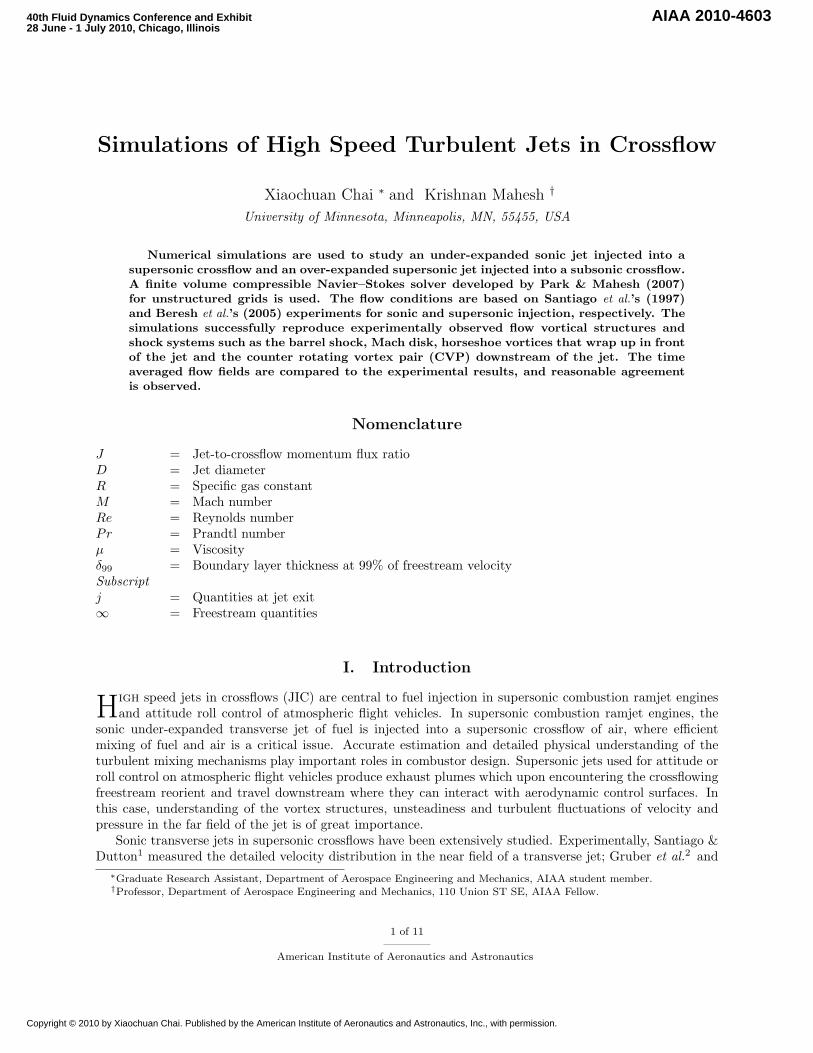
Figure 11 compares the time averaged streamwise velocity field with the experimental result. Qualita-tively, the simulation agrees with the experiment. However, in the simulation, the low u–velocity regionspreads more than the experiment, blurring the trajectory of minimum u–velocity. Figure 12 shows muchbetter result for vertical velocity field, which agrees with the experiment quantitatively. The average velocityprofiles at five different locations downstream of the jet (figure 13) show similar behavior. The peak of thestreamwise velocity deficit spreads wider than the experiment in each profile, while the shapes of v–velocityprofiles agree much better with the experiment but have slightly higher peak locations. The peak of theu–velocity deficit indicates the location of the jet core which has the largest impedance to the oncomingcrossflow, while the peak of v–velocity marks the position of the CVP which induces the v–velocity compo-nent. Both peaks are measures of the jet trajectory. The simulation predicts a slightly stronger jet core anda slightly higher jet penetration. Also observed is the decrease of these peak values along the downstreamdirection, which shows the decay of the jet as it convects downstream and mixes with the crossflow fluid.In figure 13, discrepancies of u–velocity deficit profiles are observed right above the wall, especially at thelocations nearer to the jet. This is probably due to the laminar boundary layer used for the inflow condi-tion. Turbulent inflow boundary layer can expedite the mixing of the jet and crossflow, thus will probablygive smaller u–velocity deficits near the wall at corresponding downstream locations. The overall agreementbetween the simulation and the experiment is reasonable.

9 of 11

American Institute of Aeronautics and Astronautics

y/D

[U∞(x)− u] /U∞(a)

y/D

v/U∞(b)

Figure 13. Comparisons of streamwise velocity deficit (a) and wall-normal velocity (b) between simulationand experiment at jet downstream locations x/D = 21, 26.2, 31.5, 36.7, 42.0. lines = simulation, symbols =experiment (reproduced from Ref.12).

V. Conclusions

Numerical simulations of an under-expanded sonic jet in a supersonic crossflow and a supersonic jet ina subsonic crossflow are performed to study the key physics of high speed jets in crossflows. The parallelfinite volume Navier-Stokes solver on unstructured grids developed by Park & Mahesh14 is used. Commonflow structures in the two cases include the barrel shock and the Mach disk, the separation region of inflowboundary layer in front of the jet, unsteady jet-crossflow shear layer and counter rotating vortex pair. Inthe sonic jet in supersonic crossflow, a bow shock and a separation shock are formed in front of the jetdue to the supersonic crossflow. The separation bubbles wrap up, bend around the jet and are elongatedby the crossflow, forming horseshoe vortices. The horseshoe vortices break down to smaller scale eddies asthey stretch downstream. The strong shear layer between the jet and the crossflow causes Kelvin-Helmholtzinstability. The collapse of jet-crossflow shear layer and the CVP enhance the mixing of the jet and crossflow.

In the simulation of supersonic jet in subsonic crossflow, the jet penetrates more into the crossflow dueto high momentum ratio. Secondary shocks are observed within the supersonic jet and the jet expandsand contracts accordingly. No obvious horseshoe vortices are observed from the instantaneous field. Theseparation bubbles, where the horse vortices originate, either break down before the jet or reattach to thejet boundary. Strong shear layers are observed and penetrate deep into the crossflow.

Time averaged flow fields and statistics of velocities and Mach number are computed. Reasonable agree-ment is observed between available simulation and experimental data for both cases. The presented workshows the considerable promise of our unstructured algorithm to accurately reproduce this complex flow.

Acknowledgments

This work is supported by the National Science Foundation under grant CTS-0828162 and the Air ForceOffice of Scientific Research under grant FA9550–04–1–0341. Computer time for the simulations was providedby Minnesota Supercomputing Institute (MSI), National Institute for Computational Sciences (NICS) andTexas Advanced Computing Center (TACC).

References

1Santiago, J. G., and Dutton, J. C., Velocity Measurements of a Jet Injected into a Supersonic Crossflow, Journal ofPropulsion and Power, Vol. 13, No. 2, 1997, pp. 264–273.

2Gruber, M.R., Nejad, A.S., Chen, T.H., Dutton, J.C., Large structure convection velocity measurements in compressibletransvers injection flow-fields, Exp. Fluids, Vol. 12, No.5, 1997, pp. 397–407.

10 of 11

American Institute of Aeronautics and Astronautics

3VanLerberghe, W. M., Santiago, J. G., Dutton, J. C. & Lucht, R. P., Mixing of a sonic transverse jet injected into asupersonic flow, AIAA Journal, Vol. 38, No. 3, 2000, pp. 470–479.

4Ben-Yakar, A., Mungal, M.G., Hanson, R.K., Time evolution and mixing characteristics of hydrogen and ethylene trans-verse jets in supersonic crossflows, Physics of Fluids, Vol. 18, No. 2, Feb 2006.

5Fric, T. F., and Roshko, A., Vortical structure in the wake of a transverse Jet, Journal of Fluid Mechanics, Vol. 279, pp.1–47, 1994.

6Peterson, D.M., Subbareddy, P.K., Candler, G.V., Assessment of synthetic inflow generation for simuating injection intoa supersonic crossflow, AIAA Paper, 2006-8128.

7Kawai, S. and Lele, S. K., Mechanisms of jet mixing in a supersonic crossflow: a study using large-eddy simulation, Centerfor Turbulence Research Annual Research Briefs, 2007.

8Kawai, S. and Lele, S. K., Large-eddy simulation of jet mixing in a supersonic turbulent crossflow, Center for TurbulenceResearch Annual Research Briefs, 2008.

9Kawai, S. and Lele, S. K., Dynamics and mixing of a sonic jet in a supersonic turbulent crossflow, Center for TurbulenceResearch Annual Research Briefs, 2009.

10Gruber, M.R., Nejad, A.S., Chen, T.H., Dutton, J.C., Compressibility effects in supersonic transverse injection flowfields,Physics of Fluids, Vol. 9, No. 5, May 1997.

11Beresh, S. J., Henfling, J. F., Erven, R. J., and Spillers, R. W., Penetration of a Transverse Supersonic Jet into a SubsonicCompressible Crossflow, AIAA Journal, Vol. 43, No. 2, 2005, pp. 379–389.

12Beresh, S. J., Henfling, J. F., Erven, R. J., and Spillers, R. W., Turbulent Characteristics of a Transverse Supersonic Jetin a Subsonic Compressible Crossflow, AIAA Journal, Vol. 43, No. 11, 2005, pp. 2385–2394.

13Beresh, S. J., Henfling, J. F., Erven, R. J., and Spillers, R. W., Crossplane Velocimetry of a Transverse Supersonic Jet ina Transonic Crossflow, AIAA Journal, Vol. 44, No. 12, 2006, pp. 3051–3061.

14Park, N. and Mahesh, K. 2007, Numerical and modeling issues in LES of compressible turbulent flows on unstructuredgrids, AIAA Paper–722.

15Yee, H. C., Sandham, N. D., and Djomehri, M. J. Low-dissipative high-order shock-capturing methods using characteristic-based filters, J. of Comput. Phys.–150:199, 1999.

16Sutherland, W. , The viscosity of gases and molecular force, Philosophical Magazine S. 5, 36, pp. 507-531, 1893.17Muppidi, S. and Mahesh, K., Study of trajectories of jets in crossflow using direct numerical simulations, Journal of Fluid

Mechanics, vol. 530, pp. 81–100, 2005.

11 of 11

American Institute of Aeronautics and Astronautics