simulations of contact mechanics and wear of linearly

Simulations of contact mechanics and wear

of linearly reciprocating block-on-flat

sliding test

André Rudnytskyj

Mechanical Engineering, master's level (120 credits)

2018

Luleå University of Technology

Department of Engineering Sciences and Mathematics

Simulations of contact mechanics and wear of linearly reciprocatingblock-on-flat sliding test

Andre Rudnytskyj

Master programme in Tribology of Surfaces and Interfaces - TRIBOS 4th ed.Enrollment Semester Autumn 2016.

Department of Engineering Sciences and MathematicsLulea University of Technology

©Lulea University of Technology, 2018. This document is freely available atwww.ltu.se

https://www.ltu.se/?l=en

PrefaceThis master’s thesis was carried out at the Division of Machine Elements, Depart-ment of Engineering Sciences and Mathematics of Lulea University of Technology(LTU), in Sweden. It was made possible through the Joint Erasmus Mundus Mas-ter Course (EMMC) TRIBOS (Tribology of Surface and Interfaces), of which Itook part in its 4th generation between the years of 2016 to 2018.

I would like to thank the Education, Audiovisual and Culture Executive Agency(EACEA) of the European Union and the TRIBOS programme coordinators, pro-fessors, tutors, lecturers, and everyone involved in the programme from the Uni-versity of Leeds (UK), the University of Ljubljana (Slovenia), the University ofCoimbra (Portugal), and Lulea University of Technology (LTU) for their supportinside and outside the classroom. I also thank the people directly involved in thedevelopment of the thesis for their helpful support and discussions throughout thetime of this work.

Andre RudnytskyjLulea, June 2018

I

AbstractThe use of computational methods in tribology can be a valuable approach to dealwith engineering problems, ultimately saving time and resources. In this work, amodel problem and methodology is developed to deal with a common situationfound in experiments in tribology, namely a linearly reciprocating block-on-flat drysliding contact. The modelling and simulation of such case would allow a betterunderstanding of the contact pressure distribution, wear and geometry evolutionof the block as it wears out during a test. Initially, the introduction and motivationfor this work is presented, followed by a presentation of relevant scientific topicsrelated to this work. Wear modelling of published studies are reviewed next, alongwith studies available in the literature and the goals for this thesis.

The fourth section refers to the methodology used and the built-up of themodel problem. In this work the Finite Element Method and Archard’s wearmodel through COMSOL Multiphysics® and MATLAB® are used to study theproposed contact problem. The construction of the model problem is detailed andthe procedure for wear, geometry update and long term predictions, is presentedinspired by the literature reviewed.

Finally, the results are presented and discussed; wear increment and new ge-ometries evolution are presented in the figures, followed by pressure profile evo-lution at selected times. The final geometry is also compared for different timesteps. At last, conclusions and recommendations for future work are stated.

II

Contents1 Introduction 1

1.1 Motivation . . . . . . . . . . . . . . . . . . . . . . . . . . . . . . . . 1

2 Theory & Literature Review 22.1 Tribology . . . . . . . . . . . . . . . . . . . . . . . . . . . . . . . . 22.2 Friction . . . . . . . . . . . . . . . . . . . . . . . . . . . . . . . . . 32.3 Wear . . . . . . . . . . . . . . . . . . . . . . . . . . . . . . . . . . . 42.4 Factors affecting friction and wear . . . . . . . . . . . . . . . . . . . 5

2.4.1 Contact area . . . . . . . . . . . . . . . . . . . . . . . . . . 52.4.2 Load . . . . . . . . . . . . . . . . . . . . . . . . . . . . . . . 62.4.3 Sliding velocity & Temperature . . . . . . . . . . . . . . . . 62.4.4 Running-in & Transfer-film . . . . . . . . . . . . . . . . . . 7

2.5 Wear modelling . . . . . . . . . . . . . . . . . . . . . . . . . . . . . 92.5.1 Contact modelling . . . . . . . . . . . . . . . . . . . . . . . 92.5.2 Finite Element Method . . . . . . . . . . . . . . . . . . . . . 112.5.3 Archard’s wear equation . . . . . . . . . . . . . . . . . . . . 122.5.4 Wear modelling in the literature . . . . . . . . . . . . . . . . 13

3 Research Gap 18

4 Model & Methods 194.1 Software . . . . . . . . . . . . . . . . . . . . . . . . . . . . . . . . . 194.2 Model problem . . . . . . . . . . . . . . . . . . . . . . . . . . . . . 19

4.2.1 Wear & Geometry update . . . . . . . . . . . . . . . . . . . 244.3 Long term predictions . . . . . . . . . . . . . . . . . . . . . . . . . 264.4 Methodology overview . . . . . . . . . . . . . . . . . . . . . . . . . 27

5 Results & Discussion 295.1 Contact pressure . . . . . . . . . . . . . . . . . . . . . . . . . . . . 295.2 Wear & Geometry . . . . . . . . . . . . . . . . . . . . . . . . . . . 31

5.2.1 Initial simulations . . . . . . . . . . . . . . . . . . . . . . . . 325.2.2 Finer time steps . . . . . . . . . . . . . . . . . . . . . . . . . 345.2.3 Full-scale simulation . . . . . . . . . . . . . . . . . . . . . . 39

6 Conclusions & Future works 43

III

List of Figures1 Stribeck curve showing the behaviour of friction for different lubri-

cation regimes along with scheme of physical cases; I: Boundary, II:mixed, III: hydrodynamic, IV: EHL (non-conformal contact only).Adapted from [33]. . . . . . . . . . . . . . . . . . . . . . . . . . . . 2

2 Representation of the real contact area of rough surfaces in contact,composed by a number of micro-contacts (in red) defined by ran-dom distribution of numerous small contact points, which preventsinterlocking or meshing. Side view in square and contact surfaceview in circle. Adapted from [86]. . . . . . . . . . . . . . . . . . . . 5

3 Schematics illustrating evolution of contact between a solid lubri-cant and a rough hard counterpart: from left to right - beforesliding, gradual filling of the solid lubricant in the grooves of thecounter-surface, buildup of the solid lubricant leading to self lu-brication. Note that there exists a change in roughness of bothsurfaces. Adapted from [81, 51]. . . . . . . . . . . . . . . . . . . . . 8

4 Point mass supported by spring system (a); illustration of the La-grange Multiplier Method (b); penalty spring due to penalty term(c). Adapted from [93]. . . . . . . . . . . . . . . . . . . . . . . . . . 9

5 A plate under uniaxial tension with a hole; finite element (FE) meshof the model (middle) with finer (smaller) elements in regions wherethe fields and errors are expected to be high; typical visualizationof a simulation. Adapted from [25]. . . . . . . . . . . . . . . . . . . 11

6 Wear occurs when a fragment of material detaches from an asperityduring contact. The shape is approximated as a hemisphere withradius a. Adapted from [86]. . . . . . . . . . . . . . . . . . . . . . . 12

7 Geometric model of disc brake assembly on which wear of the padwas modelled and numerically studied; Surface profile of brake padfor wear simulation. From [84]. . . . . . . . . . . . . . . . . . . . . 15

8 Left: illustration of block on plate experiment (from [28]); right:modelling of experiment - refer to text for numbered explanation. . 21

9 FE mesh for the counter surface showing finer refinement towardsregion where contact with the block occurs. . . . . . . . . . . . . . 21

10 Finalized initial FE mesh showing zoomed-in details of finer refine-ment on destination boundary (block). . . . . . . . . . . . . . . . . 23

11 High peaks and gradients of contact pressure in the block’s edgeregion, leading to the set-up of finer FE mesh. . . . . . . . . . . . . 24

12 Detail on the construction of the block’s contact boundary; higherdensity of points in the region of high pressure peaks and gradients. 25

13 Flowchart of wear computation methodology. . . . . . . . . . . . . . 2814 Pressure profile in elastic contact for different indenters (sphere, flat

die and cone). From [96]. . . . . . . . . . . . . . . . . . . . . . . . . 2915 Reference entities for non-dimensionalization of results. . . . . . . . 2916 Contact pressure profile (top) normalized by the maximum pres-

sure of the frictionless case, pr,fric (left) and x-component of thedisplacement field (bottom); frictional case with µ = 0.3 - chosenfor visualization purposes only (right). . . . . . . . . . . . . . . . . 30

IV

17 General normalized dynamic pressure profile on the block’s contactboundary for unworn sliding (moving towards the right). . . . . . . 31

18 Dynamic contact pressure peaks behaviour with regards to coeffi-cient of friction µ changes. . . . . . . . . . . . . . . . . . . . . . . . 31

19 Wear, ∆tg = 2s (“cycle-update”), A = 1000, 1st cycle. . . . . . . . . 3220 Wear, ∆tg = 2s (“cycle-update”), A = 1000, 2nd, 3rd and 4th cycles. 3321 Wear, ∆tg = 2s (“cycle-update”), A = 500, 4th cycle. . . . . . . . . 3422 Wear, ∆tg = 0.05s, A = 1000, at different moments. . . . . . . . . . 3523 Maximum dynamic pressure during simulations of 4 cycles; “*”

refers to inversion in the direction of motion when associated witha step “s”, or start of a new cycle when associated with a cycle “c”. 36

24 Dynamic pressure, ∆tg = 0.05s (named dt on the title), A = 1000,in the beginning and in the end of the same stroke moving to theright direction. . . . . . . . . . . . . . . . . . . . . . . . . . . . . . 37

25 Block’s edge final geometry after 4 cycles with A = 1000. . . . . . . 3826 Block’s edge final geometry after 4 cycles with A = 500. . . . . . . . 3827 Block’s edge final geometry after 2 cycles with A = 1000. . . . . . . 3928 Maximum dynamic pressure during simulations of first 4 cycles with

A = 4000; “*” refers to inversion in the direction of motion whenassociated with a step “s”, or start of a new cycle when associatedwith a cycle “c”. . . . . . . . . . . . . . . . . . . . . . . . . . . . . . 40

29 Maximum dynamic pressure during simulations of 4th to 9th cycleswith A = 4000. . . . . . . . . . . . . . . . . . . . . . . . . . . . . . 40

30 Step showing non-smooth wear increment during the 6th cycle withA = 4000. . . . . . . . . . . . . . . . . . . . . . . . . . . . . . . . . 41

31 Wear, ∆tg = 0.05s, A = 4000, at different moments. . . . . . . . . . 42

V

1 INTRODUCTION

1 IntroductionEssentially all contacts of solid matter involve friction and wear, from modularjunctions of hip replacement, to bearings in turbines of hydropower plants, andNASA’s Mars rover Curiosity’s wheels. Wear is a crucial factor that determinesthe service life-span and reliability of engineering systems, having enormous eco-nomical impact. In fact, a few decades ago, mechanical wear was estimated to beresponsible for a loss of as high as 6 percent of the annual U.S. gross domesticproduct [22, 69].

In such scenario, scientific and empirical efforts on expanding the understand-ing of wear processes have been made throughout the years, by mathematicallydeveloping relationships with relevant parameters in the tribological system. Suchchallenging and bold endeavours have been exposed by Meng and Ludema [56],whose work reviewed hundreds of wear and friction models from the literature. Al-though for many specific situations, models and theory have been detailed fairlywell, there is evidently no universal model applicable to all cases.

Among varied approaches to model events of the natural world, numerical mod-elling comes up as a useful, fast, cheap, improvable complement to experiments,becoming interesting tools to provide scientists with better understanding of asystem’s behaviour and events, which can result in accurate predictions providingthe model is validated. A general trend towards increased use and developmentof numerical modelling in several instances of engineering, allow its use also intribology.

1.1 MotivationWhile modelling and simulation of single-part bodies and mechanical evaluationare simulated fairly accurate, assemblies containing physical interfaces and mate-rial loss can raise the difficulty of the task. Due to the complex, multi-disciplinary,and stochastic nature of tribological processes, i.e., surface topography, frictionalheat, debris, chemical reactions, atomic interactions and so on, wear modelling isa tricky phenomenon to model, to say the least.

Despite the complexity of computational tribology yielding research in the de-velopment of numerical methods and robust algorithms themselves for implemen-tation of simple contact and friction, established computational tools are readilyavailable to model frictional contact problems. Such tools can be sufficient forstudy purposes of practical cases, bearing in mind the limitations of the modellingthe tool can provide.

Oscillatory contacts are commonly encountered in engineering applications andalso in tribology experiments; coefficient of friction and wear coefficient are oftenestimated in experiments with tribometers such as the pin-on-disc or block-on-flat(also named flat-ended pin-on-disc, [39]) tests, where a sample is pressed againsta counter-face and slide with a reciprocating (repetitive up-and-down or back-and-forth) motion. A numerical model that would capture the phenomena andevolution of events taking place in such experiments would serve as a doorwayto a better comprehension of the experiment and tribology in general, besidesimproving design capabilities, overcoming limitations of experiments and savingresources.

1

2 THEORY & LITERATURE REVIEW

2 Theory & Literature ReviewIt is essential to have a good understanding of the phenomena that may occur inthe tribological contact of a linearly reciprocating sliding system, not only for thecomprehension of the events in experiments and real applications, but also for theability to critically analyze the validity of simulations.

In this section, tribology and its relevant topics for this work are presented,followed by a brief introduction to computational tribology and a review on wearmodelling by numerical means.

2.1 TribologyTribology is the “science and technology of interacting surfaces in relative motionand of the practices related thereto” or, in other words, the study on lubrication,friction, and wear of moving or stationary parts in physical contact (essentiallyrolling, sliding, normal approach or separation of surfaces) [33, 86]. Tribologycomprises not only mechanical phenomena, but several topics in materials scienceand chemistry, making it a greatly interdisciplinary field.

The lubricant, with the general purpose of - but not limited to - reducing energyloss due to friction and reducing wear is a key part of the tribosystem. Dependingon the application, the lubricant may be solid or fluid, and the lubrication regimeis classified as: boundary, mixed (or partial), elastohydrodynamic (EHL), and fullfilm lubrication (or hydrodynamic). More details of the regimes can be found, forexample, in [86].

The German engineer Richard Stribeck, presented a useful concept to visualizethe behaviour of friction in each lubrication regime, in what became known as theStribeck curve [33]. The curve (Figure 1) present the coefficient of friction understeady state conditions as a function of the Hersey number: Hs = ηω/p, where η isthe absolute viscosity, ω is rotational speed, and p is pressure. The higher is Hs,the thicker is the film thickness between the surfaces.

Coefficien

toffriction

Hersey number orfilm parameter

Absence ofboundarylubricants

IIIII

I

IV

Figure 1: Stribeck curve showing the behaviour of friction for different lubricationregimes along with scheme of physical cases; I: Boundary, II: mixed, III: hydrodynamic,IV: EHL (non-conformal contact only). Adapted from [33].

2


In the case of rough surfaces, the Stribeck curve is commonly characterized byλ instead of Hs [86, 54], where λ is a specific film thickness with respect to surfaceroughness of the bodies; the film thickness can be determined from calculations ofEHL film in terms of dimensionless entities of speed, materials, load and geometry,famously studied by Hamrock & Downson [33].

In this work, the focus is on boundary lubrication (or boundary film lubrica-tion), which is the scenario of many practical applications such as metal-workingtools or polymer bearings in hydropower applications. This regime has as mainfeatures [36]:

• Surfaces of the bodies are in contact at microasperities, hence the load ismainly transmitted by mechanical contact resulting in stresses and deforma-tion of the body(ies);

• Tribology is defined by physical properties of the bodies, and possibly bychemical properties of thin surface films of molecular proportions (1-100nm).

2.2 FrictionFriction can be defined as the resistance encountered when one body moves tan-gentially over another with which it is in contact, being the major cause of wear[86] and energy dissipation. It is governed by processes occurring mainly in thethin surface layers of the contacting bodies and thus not an intrinsic materialproperty, but rather of the tribological system. Therefore, when studying andmeasuring friction, it is important to keep in mind its stochastic nature.

Boundary lubrication regime can be described by means of the coefficient offriction, µ, defined as

µ = FtF

(1)

where Ft is the tangential frictional force and F is the normal load to the sur-face. The nature of Ft essentially results from two major processes1 in commonmaterials:

• Adhesion, or, to be more precise, the shearing of adhesive junctions, whichare created at the interface and constitute the real area of contact;

• Deformation of the softer material caused by penetration of hard asperitiesof the mating surface, i.e., ploughing of a groove, which can be partly elasticand partly plastic, depending on the materials and roughnesses of the bodiesinvolved [48].

The idea of adhesion and deformation being non-interacting components of atwo-term model of friction is found in the literature as a convention; other authorsinclude the separation and formation of transfer film and wear debris as a thirdfactor [60, 59].

The contribution of each process to the total frictional force is a function ofseveral factors; the shearing of adhesive junctions depends, for instance, on the

1Other processes are separately considered and may be more or less important in specificcases, such as scratching, slip, or hysteresis losses [30].

3


nature of the contact, the chemistry, the stress state and so on, whereas thedeformation process is closely related to the mechanical properties of the surfaces,the sliding and environmental conditions. Adhesion can be described in terms ofsurface energy, the junction growth occurs in a limited way, but, both in polymersand metals, rupture tends to occur within the bulk of the polymer rather than atthe interface.

The general understanding of friction between unlubricated solids consists ofthree basic elements detailed by Tabor [88]: true area of contact; type and strengthof bond formed at the interface; and the manner in which the material in andaround the contacting regions is sheared and ruptured. Hence, such model assumesthat frictional effects occur in a microscale.

2.3 WearWear can be generally defined as the progressive damage to contact areas in relativemotion, causing gradual loss of material. Evidently, the factors described in theprevious subsections that affect friction will also have an effect on wear. Thereis a great diversity of mechanisms and conditions related to wear which make arigorous classification inviable.

In abrasive wear, a harder material/body removes material from a softer body,which can occur by cutting, microfracture on brittle abraded materials, pull-out ofindividual grains, or repeated deformations by subsequent grits [86]. Cutting refersto the classical model, resulting in wear grooves, micro-machining, or scratching.The abrasive particles can be present in the microstructure, enter as contaminants,or generated as wear debris, the abrasive action can be in terms of ploughing, i.e.,plastic grooving without material removal, or in terms of cutting. The process canbe thought of consisting of three stages [48]: mechanical deformation and stressesat a contact area; action of the frictional forces; rupture of material.

Adhesive wear occurs during sliding due to the continuous sticking and tearingof the adhesive junctions, thus it is related to interfacial wear and friction dueto shearing of the junctions. Abrasive wear, on the other hand, is related to theploughing phenomenon. This overview follows the concept of the two-term frictionmodel, i.e., that the energy dissipation of the two frictional terms results in twogeneral modes of damage and consequent wear: interfacial, and cohesive [12]. Thebalance between interfacial bonding and cohesive forces of the material determinehow the fracture will occur.

Repeated stressing during reciprocating can lead to subsurface crack initiationwhich may propagate parallel to the surface due to deformation. This event resultsin surface fatigue wear, a common type of wear in polymer tribological systems.Although it is regarded as a mechanical process of failure, it can also be treated as“a thermally activated failure process, where failure occurs as a result of thermalbreakdown of the chemical bonds and the magnitude of the applied stress reducesthe activation energy barrier for bond rupture ” [48]. Evidently, the intensity offailure depends on the materials involved; Smurugov et al. [83] studied how thewear rate for PTFE varies with temperature at different loads, justifying the resultsin terms of changes in the energy barrier of thermodegradation of the polymer.

Several other types and classification of wear exist, which may involve one ormore mechanisms and present resemblances with the previous discussed types.

4


Stachowiak and Batchelor [86] discuss several aspects of erosive wear, where asurface is damaged by the impact of solid or liquid particles of solid against thesurface of an object; cavitation wear, corrosive wear, oxidative wear, fretting wearand other minor mechanisms also exist [39].

2.4 Factors affecting friction and wearThe tribological system is sensitive to numerous factors, which range from materialproperties to operation conditions. The contact at the interface, its bonds andrupture are all affected by the conditions, consequently affecting friction as a whole.No single wear mechanism can completely describe wear in a tribological system;rather, different mechanisms may take place at different times and may becomemore or less important, slowly or abruptly, as the sliding conditions change. Themain important factors affecting friction and wear are considered in the followingsubsections.

2.4.1 Contact area

It is well known that the real contact area between solid bodies is generally onlya small fraction (Figure 2) of the nominal contact area [21] which determine thenature of friction and wear.

Figure 2: Representation of the real contact area of rough surfaces in contact, composedby a number of micro-contacts (in red) defined by random distribution of numeroussmall contact points, which prevents interlocking or meshing. Side view in square andcontact surface view in circle. Adapted from [86].

One of the classical friction laws2 refers to the independence of friction to thesize of the nominal contact area3. Indeed, with a large nominal contact area,the micro-contacts (or asperities) lie further apart, hence the sum of these micro-contacts, which is the real contact area, Ar, is, in this sense, independent of thenominal contact area. Greenwood and Williamson famously developed a model

2It is known that ancient civilizations had a substantial understanding of friction and tribologythrough practical problems associated thereto; empirical laws of sliding friction from what mightbe termed scientific studies of tribology, often known as Amontons’ Laws, are a re-discovery ofwork done by Leonardo Da Vinci.

3The other 2 classical friction laws are: proportionality of friction to normal load, and inde-pendence of sliding velocity, the latter added by Coulomb. They have no physical basis and areempirical observations [65].

5


for multi-asperity contact area by joining Hertzian theory of elastic contact andprobability theory, concluding that under certain conditions the ratio of contactarea and load can be found to be practically constant [31].

According to Hutchings and Shipway [39], polymers under sufficiently highloads will result in Ar being equal to the nominal contact area, allowing a directcomparison between a measured coefficient of friction and measured shear yieldstrength of bulk samples of the material. There is no general rule as to thebehaviour of friction as a function of roughness. In a polymer-on-metal contact,the metal counter-surface roughness, shape and orientation of the asperities mayplay an important role in both friction and wear. If a metal counter-surface is verysmooth, adhesion forces may become strong, whereas higher surface roughness mayresult in more abrasion [1].

In this sense, one may realize that the coefficient measured in experimentsis only a statistical average, where it is assumed a uniform distribution of shearresistance over all the contact spots, which is not the case for real interfaces.

2.4.2 Load

Another of the classical friction laws refers to the proportionality of friction tothe load. For materials with low Young’s modulus to hardness values (E/H),such as common polymers, micro-contacts will largely deform elastically, unlessvery rough surfaces are involved ([92, 39]). In such case, Ar increases by lessthan the proportional amount with the normal load, because of increasing com-pression stress in the micro-contacts, but not in the number of asperity contacts;from Hertzian contact theory [43, 31], any elastic contact in which the number ofcontacts remains constant under a compressive load F results in

Ar ∝ F 2/3 (2)

and, in the case of perfectly plastic behaviour of asperities,

Ar ∝ F. (3)

In the case of a thin polymer film between rigid surfaces, the coefficient offriction decreases with increasing normal load, which is observed in practice forpolymers which form transfer films [75]; in fact, it is expected that µ ∝ F−1/3,proportion found in fair agreement in practice for high loads or smooth surfaces[39]. In metals, on the other hand, micro-contacts’ deformation is mostly plas-tic which implies in an increase in the number of micro-contacts as the load isincreased (the yield pressure for each asperity contact becoming a material con-stant). Since adhesion is also proportional to Ar, the total friction ends up beingroughly proportional to the load [88]. Further discussion can be found in [60]. Interms of wear, the increasing load will result in higher contact pressures and shearstresses, which eventually leads to more mechanical damage.

2.4.3 Sliding velocity & Temperature

With regards to sliding velocity, ploughing and adhesion causing friction in metalsare generally independent of velocity; however, when high velocities are involved,melting of asperities may occur which lead to a dependence of the coefficient of

6


friction on velocity, decreasing with increasing sliding speeds. Furthermore, slid-ing contact in general is “distributed over a lesser number of larger contact areasrather than a large number of contact points” [86], which may be explained bygreater separation between opposing surfaces during sliding, depending on thecase. Polymers may display a strong visco-elastic behaviour, resulting in an in-crease of E at higher deformation rate [76]; hence, summits penetrate less in thepolymer decreasing ploughing friction and real contact area. It has been shown,however, that many polymers exhibit higher wear at higher sliding speeds [75].

Temperature rise normally occurs as the sliding speed increases, since the dis-sipation of the frictional energy in the rubbing is mostly in the form of heat. Inmetals, limited temperature changes (< 150°C) do not significantly change theirmaterial properties, but higher temperatures may cause changes such as decreasein hardness and melting of asperities, increase in rate of oxidation, or even phasetransformation, depending on the dissipation. In polymers, mechanical propertiesmay decline fast with temperature rise, as it transits from a “glassy state” (highstrength stiffness) to a “rubbery state” (low strength and stiffness); such softeningleads Ar to approach the nominal contact area. Hence, on one hand, tempera-ture increase might increase the contact area, but on the other it decreases shearstrength. In some thermoplastics, over a critical sliding speed, the temperature atthe interface may cause surface melting and thermal softening, leading to slightdecrease in wear rate ([1]), while in other materials, the wear rate may increasedue to higher adhesion. Evidently, the length scale being study dictates the rel-evance of the events to the general scenario; on the fine scale, for instance, therewill likely be a transformation of a contacting layer, whereas in a bigger scale,thermal stresses may relevant in the general load configuration of the system.

Temperature in tribological contacts is a complicated topic, to say the least.Peaks of temperature called flash temperature are considered to occur in the in-stantaneous true contact area due to adhesive friction in a very short period oftime. The many available models to calculate the contact temperature considerdifferent geometrical, physical, and dynamic assumptions, and can vary severalhundreds of °C among each other under the same input parameters, as studied by[44]. Measurements encounter the difficulty of not only the contact location beingenclosed between two surfaces, but also the temperature varying spot-to-spot inthe asperity micro-contacts within the same contact.

2.4.4 Running-in & Transfer-film

The initial stages of a contact between two bodies are commonly characterizedby simultaneous transitional processes occurring on different scales within the in-terface; such processes depend on how the energy in the tribosystem is dissipatedand are commonly related to friction, wear, temperature and, in some cases, third-body distribution, crystallographic orientation and state of work-hardening. Thenet result of all these processes is named running-in, or breaking-in, but the termwearing-in refers to when the wear rate during the early life of a machine compo-nent is changed due to geometrical changes. Hence, running-in, besides possiblyinvolving wearing-in, also includes changes in friction that do not necessarily takeplace over the same period of time as wearing-in; further discussion on this issuecan be found in [10].

7


The sliding process can generate third-body material primarily from the softerbodies, which can be pushed out of the contact interface (wear debris), or betransferred to the harder counterpart and adhered to the surface. In a contactinvolving polymers (but not exclusively), a phenomenon of material transfer, usu-ally referred to as transfer film formation (or third-body layer), may occur atthe interface of the contact affecting the tribological behaviour of the pair. Aspolymer particles are worn out, depending on the static electric attraction, me-chanical embodiment and sliding conditions of some materials, they form strongadherence to the counter-surface at favourable points due to van der Waals forces,Coulomb electrostatic forces, and chemical bonding [26]. This transferred filmincreases with the steady rubbing motion resulting in changes in friction and wearby means of shielding of the soft polymer surface from the hard metal asperities,which also play a role in the process by interlocking polymer fragments [41, 6, 49].Hence, the film formation is governed by the material composition, counter-surfacecharacteristics and sliding conditions [95].

The capacity to transfer microscopic amounts of material to the mating sur-face creating a film that provides lubrication and reduces friction is known asself-lubrication (Figure 3). The stages of an ideal tribofilm formation is presentedby [26, 2]: initially there is slight chemical modification in a non-equilibrium zone;then, an elastoplastic tribofilm is formed, which may involve wear; finally, a sus-tainable tribolfilm is continuously removed and formed during sliding achievingself-lubrication. The behaviour of the transfer is reviewed by [12], dealing withwhether the transfer is isothermal or adiabatic, and whether there might be soften-ing, chemical change, morphology change (smooth or lumpy layer), or degradationin the transfer layer.

Figure 3: Schematics illustrating evolution of contact between a solid lubricant and arough hard counterpart: from left to right - before sliding, gradual filling of the solidlubricant in the grooves of the counter-surface, buildup of the solid lubricant leading toself lubrication. Note that there exists a change in roughness of both surfaces. Adaptedfrom [81, 51].

In a sense, the phenomenon of transfer film formation can be seen as a wearprocess, desirable in some applications [7]. The interfacial processes due to ad-hesion and related to the transfer film are temperature rise, polymer softening,melting, deformation, diffusion, and degradation. It is important to highlight thatthese many phenomena may occur simultaneously at the contact.

Remark 1. Other factors such as size of wear particles, humidity of theenvironment, surface energy of the materials involved in the tribosystem, fatigue,and the presence of other particles may all play a smaller or bigger role in frictionand wear.

Remark 2. Accurate and repeatable friction coefficient measurement is achallenging task, not only due to the non-equilibrium stochastic nature of the

8


sliding friction that leads to wear, but also due to the common lack of assessment(or at least presentation of assessment) of experimental uncertainty associatedwith the instrumentation. These uncertainties comprises several factors such asmisalignment of transducers’ axis, force calibration, or voltage measurements, be-sides the measurand itself [78, 13, 61]. Furthermore, discussion on how commona steady-state of wear is can be found in [9].

2.5 Wear modellingWear modelling involves a few tasks, such as finding pressure distribution anddeformation, depending on the intended approach. Initially, the contact problemneeds to be described and solved, which may involve descriptions such as the Win-kler model [68], or by the use of half-space theory [3]. Next, a method to solvethe equation must be employed, and again, a few options are available such as theBoundary Element Method, Fourier Transforms techniques, or the Finite ElementMethod. At last, the setting of the wear model is done, for which a common start-ing point is Archard’s wear equation. The chosen approach will define the amountof programming work; well-established methodologies with slight modificationsare easily employed in practical problems by means of commercial software, whilemore state-of-the-art methods make use of more idealized problems to study meth-ods and assumptions themselves, demanding more or less computational and/ormathematical development by the researcher.

The fundamentals of contact modelling can be found in the well-known bookContact Mechanics by Johnson [43], and the numerical part can be found, forinstance, in [93, 3]. A brief overview of the relevant concepts for this work ispresented in the following subsections, followed by the literature review of scientificarticles that inspired the approach detailed in the next section.

2.5.1 Contact modelling

A straightforward introduction to the formulation of contact is presented by [93]and it is useful to transcribe part of it in this subsection. Consider a mass munder gravitation load and supported by a spring with stiffness k, as illustratedin Figure 4-a.

𝑢 ℎ

𝜆𝜖

𝑎) 𝑏) 𝑐)

Figure 4: Point mass supported by spring system (a); illustration of the Lagrange Mul-tiplier Method (b); penalty spring due to penalty term (c). Adapted from [93].

9


The energy of the system, E, can be written as a function of the movement uas

E(u) = 12ku

2 −mgu (4)

for which the extremum can be found by variation, i.e., applying the principle ofminimum total potential energy, we have

δE(u) = kuδu−mgδu = 0. (5)

The second variation of E(u) results in k, which shows that the extremum ofEq. (4) is a minimum at u = mg/k. The restriction of the motion of the mass bythe rigid support is expressed by

c(u) = h− u ≥ 0 (6)

which means that for c(u) > 0 there is no contact, and for c(u) = 0 the contactoccurs. However, the variation δu is constrained by the contact surface, which fromEq. (6) yields that the virtual displacement is constrained and can only point inthe upward direction, i.e., δu ≤ 0. Hence, using the variation in the variation formin Eq. (4) we have the following variational inequality

kuδu−mgδu ≥ 0 (7)

which characterize the solution of u. At this point, special methods can be em-ployed to solve the problem.

Recalling that once the contact has been established, a reaction force (R) willappear, the contact problem where the motion is restrained by Eq. (6) can besummarized as

c(u) ≥ 0, R ≤ 0 and Rc(u) = 0 (8)

which are known as Hertz–Signorini–Moreau conditions in contact mechanics. Inthe theory of optimization, such conditions coincide with Kuhn–Tucker comple-mentary conditions. The development above can be performed to include frictionin the contact as well. In classical contact mechanics, the reaction force is assumedto be negative, i.e., only compression is considered.Lagrange Multiplier Method. The contact problem constrained by an inequal-ity can be approached by using the method of Lagrange multipliers (Figure 4-b).In this method, a term containing the constraint, which is equivalent to a reactionforce, is added to the energy equation

δE(u, λ) = kuδu−mgδu+ λc(u) = 0. (9)

The variation of equation Eq. (9) results in two equations, since δu and δλcan be varied independently, one representing the equilibrium and the other rep-resenting the kinematic constraint. Thus, the variation is no longer restricted andthe Lagrange multiplier λ can be solved, since it is equivalent to the reaction forceλ = kh −mg = R. The solution of λ needs to fulfill the requirement of R ≤ 0,otherwise the contact is inactive and the solution is simply computed from Eq. (5).

10


Penalty Method. In this approach, a so called penalty term is added to theenergy equation for an active constraint

δE(u, λ) = kuδu−mgδu+ λc(u) = 0. (10)

The penalty parameter ε can be interpreted as a spring stiffness in the contactinterface. The variation of the equation results in

kuδu−mgδu− εc(u)δu = 0 (11)

from which the solution and hence, the constraint are

u = mg + εh

k + εc(u) = h− u = kh−mg

k + ε. (12)

Recalling that for contact we have mg > kh, this implies that penetration(depending on the penalty parameter) of the point mass into the rigid supportoccurs, which is physically equivalent to the compression of the spring (Figure 4-c). Mathematically, the correct solution is approached as ε → ∞, which impliesc(u)→ 0, hence fulfilling the constraint equation.

It is important to highlight that both formulations exist in the normal andin the tangential direction of contact surface, which allows their computation incases of rough contact with friction.

2.5.2 Finite Element Method

Partial differential equations (PDEs) are mathematical representations of the lawsof physics for space- and time-dependent situations. Analytic solutions are avail-able only for a handful of cases, so approximations of the equations are performedfor general cases.

Figure 5: A plate under uniaxial tension with a hole; finite element (FE) mesh of themodel (middle) with finer (smaller) elements in regions where the fields and errors areexpected to be high; typical visualization of a simulation. Adapted from [25].

The Finite Element Method (FEM) is a numerical method to compute approx-imations of PDEs; it generates solutions of boundary value problems in a weak

11


form, i.e., integral expressions obtained by the minimization of energy functions,using variational principles, or residual methods.

The approximation is based on the division (discretization) of the continuumdomain into geometric entities named elements containing vertices named nodes,forming a mesh. The unknown field of interest - for instance, displacement fieldin a structural analysis - is piece-wise approximated by means of shape functionsdefined over each element and expressed in terms of nodal values. In other words,the field is built in the interior of elements by interpolation of the nodal values,which are obtained by solving the discretized problem. Figure 5 illustrates howa continuum domain is discretized and the result one can expect to see after asimulation, making use of a symmetry of the particular case to reduce the com-putational costs. In this manner the FEM allows to solve complex engineeringproblems in several areas of interest, which includes objects in arbitrary shape.

A general contact algorithm in a FE software consists of an initial searchalgorithm that identifies the penetration and then the satisfaction of the kinematicconditions, as described in the previous subsection. Commercial software offer suchmethods.

2.5.3 Archard’s wear equation

Once the contact problem is solved and information on contact pressure distribu-tion is available, the variable can be used as input to wear models. One of the mostfamous mathematical wear description of a sliding system was developed by Holmand Archard in the 1950s and is commonly known as Archard’s wear equation (orArchard’s law). It is arguably the most fundamental yet empirical model of wearand has become a standard in the field of tribology.

𝑣 𝑣

2𝑎

Figure 6: Wear occurs when a fragment of material detaches from an asperity duringcontact. The shape is approximated as a hemisphere with radius a. Adapted from [86].

Considering adhesive type of wear, the model assumes that sliding sphericalasperities deform plastically in the contact, which have yielding limit as a hardnessH. Hence, the mean contact normal load can be written as

dW = Hπa2 (13)

where a is the radius of the contact area. It is assumed that a hemisphere-shapedparticle (Figure 6) with volume 2πa3/3 gets loose after sliding a distance of 2awith a probability of P . The wear volume per sliding distance is then

dV

ds= P2πa3

6a = Pπa2

3 = PdW

3H . (14)

12


By integrating with respect to the sliding distance, the total wear volume V ,can be expressed as function of the load, sliding distance and hardness as

V = KWs

H. (15)

Notice that we introduced K = P/3, which is known as the dimensionlesswear coefficient, commonly obtained experimentally and used to characterize thematerial wear [91]. An analogous development can be made to obtain a similarexpression to Eq. (15) for abrasive wear, where the wear volume is analyzed froma conical penetration approach. K can be interpreted in many ways: as theprobability that the encounter of two asperities will originate a debris - and so,notice that Archard’s model is essentially probabilistic -, as the ratio of the volumeworn to the volume deformed, as a factor reflecting the inefficiencies associatedwith the various processes involved in generating wear particles and others [74,35].

Introducing the dimensional wear coefficient k = K/H (which is named specificwear rate [92]) and dividing Equation (15) by the area, an expression to calculatewear locally if the contact pressure is known is obtained:

h = kps (16)

where h is wear depth at the surface, p is the contact pressure, and s is the slidingdistance. Furthermore, wear is a dynamic process and a wear rate equation can besimply obtained by deriving Eq. (16) with respect to time, getting the slip velocityvs in the equation. In simple terms, if the contact pressure and velocity vary intime, we write

dh(t)dt

= kp(t)vs(t). (17)

Evidently, Eq. (17) is a simplification of a process that was discussed (sub-section 2.4) to be a function of many factors. Nevertheless, it is a continuousdescription of the process that can be very useful as a starting point in numericalmodelling. Clearly, Eq. (17) can be made more complex by adding effects of otherphenomena such as presence of lubricants or oxidation, for instance.

2.5.4 Wear modelling in the literature

In the reviewed literature, Johansson [42] was one of the first authors to eval-uate wear in a numerical simulation; using the Finite Element Method (FEM),the contact pressure between two elastic bodies as the material is worn out byfretting4 was studied, presenting the governing equations in a discretized versionand calculating the wear locally using Archard’s law. Debris or third body are notaccounted for, i.e., the particles disappear when formed from the geometry.

As mentioned in the beginning of this section, the implementation of the wearmodel can be performed in a variety of ways, requiring more or less mathematicaldevelopment by the researcher; a few examples are: Sawyer [77] presents closed

4Process in which two contacting bodies are subjected to slight relative vibratory motion, e.g.riveted joints.

13


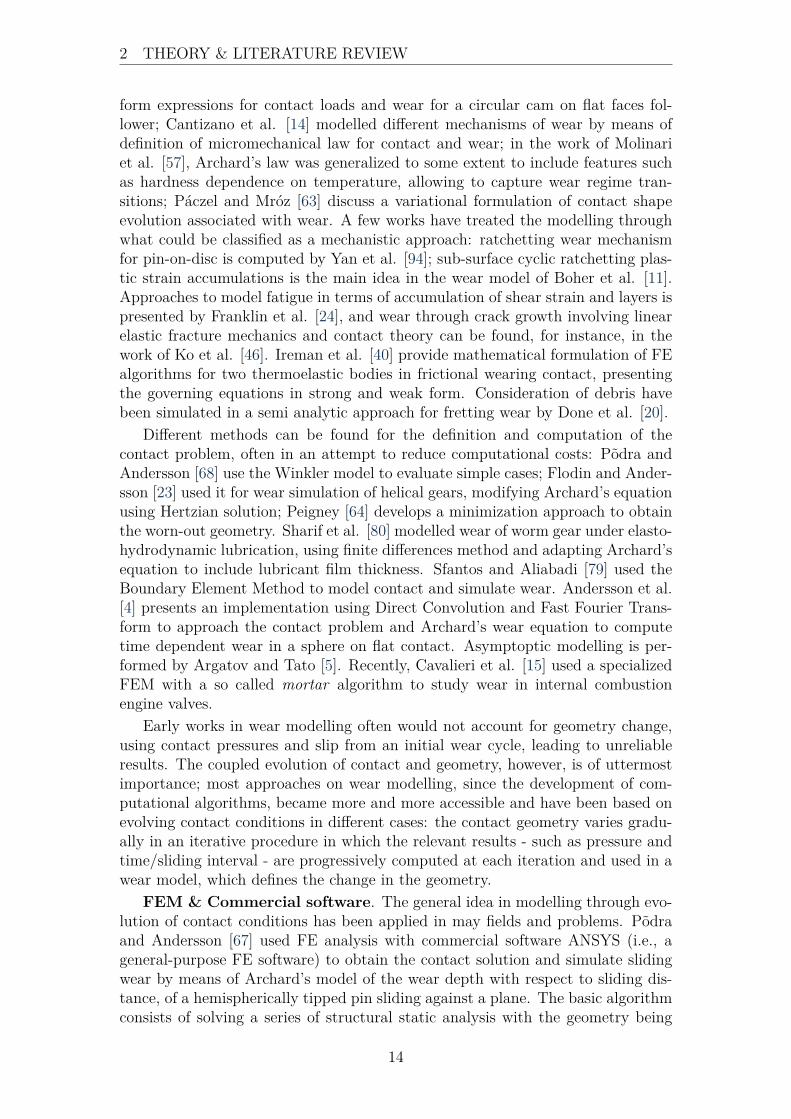
form expressions for contact loads and wear for a circular cam on flat faces fol-lower; Cantizano et al. [14] modelled different mechanisms of wear by means ofdefinition of micromechanical law for contact and wear; in the work of Molinariet al. [57], Archard’s law was generalized to some extent to include features suchas hardness dependence on temperature, allowing to capture wear regime tran-sitions; Paczel and Mroz [63] discuss a variational formulation of contact shapeevolution associated with wear. A few works have treated the modelling throughwhat could be classified as a mechanistic approach: ratchetting wear mechanismfor pin-on-disc is computed by Yan et al. [94]; sub-surface cyclic ratchetting plas-tic strain accumulations is the main idea in the wear model of Boher et al. [11].Approaches to model fatigue in terms of accumulation of shear strain and layers ispresented by Franklin et al. [24], and wear through crack growth involving linearelastic fracture mechanics and contact theory can be found, for instance, in thework of Ko et al. [46]. Ireman et al. [40] provide mathematical formulation of FEalgorithms for two thermoelastic bodies in frictional wearing contact, presentingthe governing equations in strong and weak form. Consideration of debris havebeen simulated in a semi analytic approach for fretting wear by Done et al. [20].

Different methods can be found for the definition and computation of thecontact problem, often in an attempt to reduce computational costs: Podra andAndersson [68] use the Winkler model to evaluate simple cases; Flodin and Ander-sson [23] used it for wear simulation of helical gears, modifying Archard’s equationusing Hertzian solution; Peigney [64] develops a minimization approach to obtainthe worn-out geometry. Sharif et al. [80] modelled wear of worm gear under elasto-hydrodynamic lubrication, using finite differences method and adapting Archard’sequation to include lubricant film thickness. Sfantos and Aliabadi [79] used theBoundary Element Method to model contact and simulate wear. Andersson et al.[4] presents an implementation using Direct Convolution and Fast Fourier Trans-form to approach the contact problem and Archard’s wear equation to computetime dependent wear in a sphere on flat contact. Asymptoptic modelling is per-formed by Argatov and Tato [5]. Recently, Cavalieri et al. [15] used a specializedFEM with a so called mortar algorithm to study wear in internal combustionengine valves.

Early works in wear modelling often would not account for geometry change,using contact pressures and slip from an initial wear cycle, leading to unreliableresults. The coupled evolution of contact and geometry, however, is of uttermostimportance; most approaches on wear modelling, since the development of com-putational algorithms, became more and more accessible and have been based onevolving contact conditions in different cases: the contact geometry varies gradu-ally in an iterative procedure in which the relevant results - such as pressure andtime/sliding interval - are progressively computed at each iteration and used in awear model, which defines the change in the geometry.

FEM & Commercial software. The general idea in modelling through evo-lution of contact conditions has been applied in may fields and problems. Podraand Andersson [67] used FE analysis with commercial software ANSYS (i.e., ageneral-purpose FE software) to obtain the contact solution and simulate slidingwear by means of Archard’s model of the wear depth with respect to sliding dis-tance, of a hemispherically tipped pin sliding against a plane. The basic algorithmconsists of solving a series of structural static analysis with the geometry being

14


updated due to the calculated wear depth. Issues regarding the size of wear incre-ment are mentioned. The authors also presented a version which included surfacetopography on the wear model by means of linearisation of the Abbot curve [66].Oqvist [62] performed a similar study, but also accounting for elastic deformationin the contact zone.

Yan et al. [94] present a 2D computational approach to predict the slidingwear in terms of accumulated ratcheting strain in a loaded spherical pin con-tacting a rotating disc (pin-on-disc), idealizing the problem as a 2D plane strainapproximation, thus reducing computational costs. By using a static 3D simula-tion, a conversion factor for the wear rate associated with a 3D sliding contact isintroduced.

Hegadekatte et al. [35] developed a wear processor along with commercial FEpackage ABAQUS for dry sliding wear, using Euler integration for the wear overthe sliding distance, so the simulation also works as a series of static simulationswith updated geometry; the author highlights care taken with the wear direction:nodes are shifted inward a surface normal direction, defined by the edges of theadjacent finite elements. Later, Hegadekatte et al. [34] used their algorithm tosimulate the wear of a micro-planetary silicon gear train.

McColl et al. [55] employ a 2D FE model in ABAQUS to study frictionalcontact of a cylinder-on-flat fretting test, using a modified version of Archard’sequation for sliding wear. The FE mesh at the contact is as fine as 10 micrometers.Gonzales et al. [29] simulated the experimental pin on disc tests of an Al–Li/SiCcomposite using ABAQUS, using an isotropic thermo-elastoplastic, but a simpli-fied 2D analysis.

Figure 7: Geometric model of disc brake assembly on which wear of the pad was modelledand numerically studied; Surface profile of brake pad for wear simulation. From [84].

Soderberg and Andersson [84] studied the pad-to-rotor interface of car discbrakes as a conformal dry sliding contact (Figure 7) to calculate pressure andwear; they used ANSYS and the macro scale, phenomenological Archard’s wearlaw. Only wear at the pad was considered and the sliding distance was calculatedfrom a rigid displacement. The pad is assumed to wear perpendicular to the matingrotor surface (which is rigid); this is an important and interesting assumption,because it facilitates the geometry update algorithm; they do make a remark onthis matter: “A more correct procedure would be to assume that the pad surfaceis worn in the inwards direction of its local surface normal, which may vary overtime due to uneven wear over the contact surface. The simplification is justified bythe fact that the two contact surfaces are initially flat and conformal, and that the

15


expected wear depth is much smaller than the dimensions of the contact surface.”.They use the same approach as Podra and Andersson [67], which is similar toHegadekatte et al. [35] and Oqvist [62], i.e., it works by looping through a seriesof static structural analyses of the FE model, each with an updated geometry ofthe pad surface, but without FE re-meshing between steps. Another factor thatmay influence the accuracy of the result is the step length during the numericalintegration of the wear equation. The accuracy of the solution obtained can beevaluated by comparing solutions with different step lengths.

Numerous simulations. In general, wear occurs slowly, but the linearisationof the process using Archard’s wear equation and the approach of incrementallysimulating the coupled contact and geometry can lead to high computational costswhen performing numerous simulations. Therefore, it becomes desirable to per-form extrapolations on the simulations, raising issues on the reliability of theresults, briefly highlighted by Dickrell et al. [19]. The approach on this matterdone by Kim et al. [45] in simulating a block-on-ring experiment is done by assum-ing that the contact pressure of a single FE analysis is constant for several cycles:initially, a single oscillation cycle is discretized into Ns number of steps, on whichthe wear model is computed; then, it is assumed that No oscillation cycles behavein the same way. Next, after performing NFE FE analyses, the results would berepresenting NFE ×No experiments. Finally, assuming that at this stage a steadyprogression of wear occurs, the wear depths are linearly extrapolated Nc times,corresponding to NFE ×No ×Nc cycles.

Mukras et al. [58] uses an extrapolation scheme by including an “extrapola-tion factor” to the incremental wear depth calculation, projecting the wear of acycle to several cycles. A condition is placed (and justified) such that the overallsmoothness of the pressure distribution should remain. The approach used bythe authors is discussed again in the next section. The authors also proposed aprocedure to use an adaptive factor in order to try to find a optimum value foreach cycle, in terms of deformation and contact characteristics.

Chongyi et al. [16] studied a wheel/rail wear profile using Archard’s law ina spinned 2D axisymmetric model in ABAQUS software, using limitations orsmoothing in order to avoid unrealistic scenarios, i.e., “to get better approxima-tions of the continuous wear process with a discrete sequence of profile updates”.In order to do that, a cubic spline interpolation algorithm is applied on the weardistribution before starting a new iteration of the process. Another interestingaspect is the use of bilinear elastic–plastic constitutive material model.

Other interesting works. Rezaei et al. [73] studied polymeric compositejournal bearings with ABAQUS, modelling an orthotropic material and validat-ing through experiments. In a subsequent work, Rezaei et al. [72] simulated wearfollowing the general idea of evolving contact conditions, which they named “adap-tive wear simulation”. The wear direction, i.e., sweeping of FE nodes in the inwardnormal direction was detailed following the same idea as Hegadekatte et al. [35].Rezaei et al. [72] was presumably the first to simulate wear using a non-isotropicmaterial model. They also applied a pressure and velocity dependent wear coeffi-cient. In a flat on flat sliding simulation they applied a constant pressure on thecontacting surface, instead of taking it as output.

Konya and Varadi [47] studied wear of polymer-steel sliding pin on disc pair,considering temperature and time-dependent behavior of polymer materials; in

16


their algorithm, the thermal expansion of the polymeric pin is considered in thewear increment, having an opposite effect to the wear until a steady state isreached. Martınez et al. [53, 52] also performed wear modelling in polymer-metalcontact, using an experiment-fitting power law for the wear model, performingdifferent simulations to extrapolate the model for large cycles. However, linearelastic material model was used.

When using general-purpose FE software, the possibility of using coupledthermo–mechanical analysis is eased, which can be used for instance to include theeffects of frictional heating. Shen et al. [82] performed a 2D thermo-mechanicalsimulation in ABAQUS of a spherical plain bearing with a self lubricating compos-ite liner. The consideration of the thermal analysis was performed by translatingthe temperature distribution into body loads. Lengiewicz and Stupkiewicz [50] de-veloped a general periodic pin-on-flat wear problem, considering wear on both con-tacting bodies. Gui et al. [32] studied thermo-mechanical simulations in a brakesystem. Zhang et al. [95] studied the tribological properties of self-lubricatedpolymer steel laminated composites and simulated the thermal expansion of thesolid lubricants. In their experiments, they calculated the wear coefficient bas-ing on wear marks and geometrical features. In their simulations, the transienttemperature field was studied with the account of a few assumptions so that theconservative law of energy was applicable; material properties were independentof temperature.

The general methodology with slight modifications has been applied to manydifferent problems: cam-followers works [37, 38, 85], wear of artificial cervical discs[8], wear in total disc replacements [71], wear and tribofilm growth [3], machiningtools [70], and press hardening tools [18].

17

3 RESEARCH GAP

3 Research GapIn section 2, it was shown that there are many events occurring in a tribologicalcontact which are dependent on many physical phenomena. Numerical modellingis a powerful tool that can be used to try to model such events and make pre-dictions possible. It was seen in the literature review that many simplificationsmust be performed to make simulations feasible to be analyzed; depending on theapproach, published studies focus on a practical problem using more establishedmethodologies or evaluate the numerical method itself.

In context of dry sliding, frictional contact and wear, the main goal of thisthesis is to analyze a practical problem. The objective can be stated as: the devel-opment of a numerical model and method to predict contact pressure distribution,wear and contact geometry evolution of a linearly reciprocating block in contactwith a flat plane. In the reviewed literature, no work on modelling was found toapproach this particular problem, although the general methodology of progressivecomputation of contact parameters in a iterative fashion is applicable to it.

Contact pressure and local wear during sliding is not something easily mon-itored during an experiment, thus, real time information about these entities’distributions in such cases are a valuable result intended from this work. Suchinformation would result in a better understanding of the linearly reciprocatingdry sliding contact. The scope of the thesis is subjected to the time-span available,thus defined to be limited to simulating the above mentioned entities consideringonly solid mechanics and contact mechanics physics, intended to be a first stagemodel of the proposed case.

The questions expected to be answered regard not only how the evolution of theentities occur, but also how to set up a methodology using available software. Thedevelopment of the model is described in section 4 along with the assumptions andapproximations, which can be critically analyzed with the theoretical knowledgepresented in the next section.

18

4 MODEL & METHODS

4 Model & MethodsIn this section, the tools used and the details on the development of the modelare presented. Initially, the tools and model problem are presented along with therelevant aspects and considerations used. Secondly, the employed methodologyfor wear and geometry update inspired by the literature review is presented.

4.1 SoftwareEach approach in contact mechanics and wear modelling may have its advantagesand disadvantages in terms of accuracy and computational cost [58]. A commonapproach is to use the Finite Element Method, by means of general-purpose com-mercial software. Although it has the disadvantage of being time-consuming, FEMis a powerful tool to solve contact problems and it is the approach used in thiswork. It is important to highlight that such approach involves explicitly modellingof the geometry, setting up the materials, physics, FE mesh and so on to obtainthe solution at the contact.

In this work, COMSOL Multiphysics® 5.3 and LiveLink™ for MATLAB® arethe software used. COMSOL Multiphysics® is a finite element analysis simulationsoftware, which allows coupling of systems and physics [17]. Among the severalmodules, the Structural Mechanics Module allows the static and dynamic analysisof mechanical systems, i.e., a wide range of analysis types, including time studiesin stationary or transient regimes, eigenmode/modal analysis, parametric, quasi-static, frequency-response, buckling, and prestressed. LiveLink for MATLAB ex-tends the COMSOL modeling environment with an interface between COMSOLMultiphysics® and MATLAB®, which may be used to control the software ex-ternally, i.e., through the scripting programming in the MATLAB environment,handling the COMSOL model in preprocessing, manipulation, and postprocessing.

The simulation workflow in COMSOL basically goes through the followingsteps: set up of the model environment, creation of geometric objects, specificationof material properties, definition of physics and boundary conditions, creation ofFE mesh, computation, and post-processing. Evidently, the settings of each stepshall be performed in order to best model the problem in hand, which will bediscussed in the next subsection.

4.2 Model problem3D modelling has the advantage of considering a correct geometry (dimensions,surface topography, degrees of freedom) and ability to calculate stresses and strainsin the entire bodies. However, 3D-FE models demand very high computationalcosts and processing times, which turns out to be a disadvantage when method-ologies are being studied and parameters are being varied.

Considering the problem is a first stage model and the methodology for wear isto be studied, which involves experimenting with different numerical parameters,the block in linear reciprocating motion in contact with a flat plane is approxi-mated by the use of a 2D space dimension. Among the interfaces available in theStructural Mechanics Module, the Solid Mechanics interface is used, which canprovide information on displacements, stresses, and strains of the simulation.

19

4 MODEL & METHODS

The 2D approximation can be performed using plane strain or plane stressconditions. In plane stress, the normal stress and the shear stresses directedperpendicular to the plane of study are considered to be zero. Hence, this conditionis appropriate for bodies whose thickness is small. In plane strain, the normalstrain and the shear strains on the plane of study are assumed to be zero, whichis appropriate when the out of plane dimension is much larger than the other two[27]. In the modelling of this work, the plane strain condition is used. Additionally,no inertial terms are included in the time domain analysis.

The linearly reciprocating block in contact to a flat plane is modelled, essen-tially, as two bodies (the block and the counter-surface, Figure 8) and simulatedin two study steps in COMSOL: a Stationary and a Time Dependent. Solvingthe problem in these two steps is - besides a good approach in assuring the com-putation will likely be successful at the end (in terms of solver convergence) - inaccordance to the actual experimental case; initially, the sample block is positionedand the static load is slowly applied before the movement starts.

From the “point of view” of the software, every surface of an object can comein contact to every other surface, so defining a Contact Pair under Definitions isimportant for better computational efficiency, because then the software can limitits analysis operation of contact search. Contact is typically seen as one-sidedrigid constraint; the contact algorithm in COMSOL constrains the destinationboundaries so that they do not penetrate the source boundaries. As a generalrule, one should make the stiffer object the source object or, if the stiffnesses aresimilar, make the concave side the source.

The contact feature5 makes the studies geometrically non-linear6. Commonly,strain calculations are treated in a geometrical linear fashion, i.e., the equilibriumis formulated in the underformed configuration and is not updated with deforma-tion. This implies small errors, but which are not so big to the point of justifyingthe implementation of a more mathematically complex equilibrium model, in gen-eral cases. In the case of contact physics, however, it cannot be used in a linearcontext [87]. Fortunately, COMSOL is equipped to deal with such cases.

Table 1: Material properties in the model, Thordon’s properties obtained from [90] andsteel data from COMSOL’s material library.

Block Counter-surfaceYoung’s modulus [GPa] 2.41 205Poisson’s ratio [-] 0.39 0.28Density [kg/m3] 1400 7850

Once the geometry is defined, the materials can be added to the components.The Thordon Bearings’ product ThorPlas®, a homogeneous, self-lubricating ther-moplastic material designed to operate in high pressure environments such ashydro-turbine wicket gate in hydropower plants [89], is the material used for theblock. The reason for this choice is due to internal interest on this material atthe university. The material chosen for the counter-surface is the steel AISI 4340.

5Applicable only to solid elements in COMSOL.6When geometric nonlinearity is included in structural analysis, the COMSOL automatically

makes a distinction between Material and Spatial frames. The material frame corresponds to theundeformed configuration, while the spatial frame corresponds to the deformed configuration.

20

4 MODEL & METHODS

The important material properties are shown in Table 1. For simplicity a linearelastic model was used as material model for the block.

With the aid of Figure 8, the numbered aspects and boundary conditions aredetailed for the contact analysis; the bottom region of the counter-surface is sup-ported by the machine. Hence, a boundary condition of fixed constraint 1 isapplied to the bottom of the counter-surface, which means that all translationsand rotations are zero on that boundary.

xy

1

2

5

4

3

Figure 8: Left: illustration of block on plate experiment (from [28]); right: modelling ofexperiment - refer to text for numbered explanation.

The counter-surface geometry is built in such a way that allows an appropriatepreparation for the simulation in terms of FE mesh. A division of the domainis performed 2 for meshing purposes, although it consists of the same body.Recalling that the FEM approximates the solution by means of discretization ofthe domain of interest, the accuracy of the solution is linked to the mesh size,and so, it is important to have a sufficiently fine discretized mesh of the domain7.Figure 9 shows the FE mesh for the counter-surface.

Figure 9: FE mesh for the counter surface showing finer refinement towards region wherecontact with the block occurs.

The modelling of the contact was performed in such a way that the bodiesare not in contact in the initial configuration, i.e., a gap 3 exists between theblock and the counter-surface. The reason is that when wear occurs, regionspreviously in contact will not be in contact anymore, so there will be a creationof a gap. Thus, the modelling needs to be able to deal with a contact modellingof bodies which might not be in contact at the start of the simulation. As aconsequence, the block is initially unconstrained and there will be possible rigidbody displacements, which often causes the solver to fail. This issue is avoided inthe load and displacement boundary conditions.

7Theoretically, as the mesh size approaches zero, the solution approaches the exact solution,but limitations with regards to finite computational resources and time exist. Thus, the goalof a simulation is to minimize the difference (“error”) between the exact and the approximatedsolution, according to some accepted tolerance criterion.

21

4 MODEL & METHODS

A rigid connector feature is used on the top of the block 4 . Rigid connectorsare boundary conditions for modelling rigid regions; the selected boundaries willbehave as a single rigid object. In reality, the load on top of the block is appliedby the steel parts of the machine, and thus the rigid connector is appropriate inthis case not only because the stiffness of the steel is much larger than the block’smaterial, but also and more importantly because it simplifies the simulation. Next,a functionality of an applied (parameterized) force is added to the rigid connectoron the top of the block.

Another rigid connector 5 is used in the upper parts of the block’s sideboundaries - steel parts of the machine contact the sample block at those locationsin the actual case - in order to apply the displacement for the Time-dependentstudy. The displacement was imposed using an expression of a wave functionglobally defined to represent the oscillatory linear motion, which can be expressedas a function of time according to

u(t) = A sin (ωt+ φ) (18)

where A is the amplitude of the displacement - half the stroke - ω is the angularfrequency of the motion, i.e., in [rad/s], and φ is the phase, which is useful todefine the starting position of the block in the simulation (providing initial valuesof displacement field are also defined).

In a two step simulation, the initial values of the second step should be con-sistent with the final solution of the first step. Hence, a global parameter t = 0 isdefined to be used in the Stationary study step, which results in no displacementsfrom the displacement function dependent on t.

Another important aspect refers to the initially unconstrained problem; aSpring Foundation feature is added to the boundaries of both 4 and 5 , whichare in essence, a temporary weak spring during the beginning of the simulation.With the springs present, the rigid body motions are constrained, hence the prob-lem can be solved. In order for them to not affect the actual configuration ofthe problem, a parameter Par ranging from 0 to 1 is used to define a stabilizingspring’s stiffness ku as

ku = k0(1− Par)× 2−(Par×10) (19)

which results in the stiffness reducing to zero as the parameter reaches 1. k0must be chosen in such a way that the spring force balances the external load ata sufficiently small displacement; “a too weak spring will give a too large initialoverclosure of the contact boundaries, and a too stiff spring might influence thesolution too much” [17]. In this modelling, the value was chosen at 106N/m. Thisapproach avoids the rigid body displacement that could occur on the block.

The load applied at 4 is also parameterized. In order to “help” the soft-ware converge better, it is useful to start the iteration close enough to the solu-tion (Newton-Raphson or similar methods are used); this is done by ramping theboundary condition, in this case, the compressive load. So, a small load can beapplied and once the simulation has converged, we use the solution as a startingpoint when iterating for a higher load until the desired load has been reached.This is done with the parameterization Par × Load and in adding a auxiliarysweep in the solver of the software. Thus, the same parameter Par is used for

22

4 MODEL & METHODS

both the spring foundation and the load, when it reaches 1, the load is the desiredload, and the spring acts no more, as intended initially.

Once contact occurs, the contact constraint is enforced. There are two waysof enforcing contact constraint, as presented in the previous section; the first oneis the Penalty method, which can be seen as a spring that applies compressiveforce in which the pressure is the penaltyfactor×penetration, being relatively lessaccurate, but more robust and requires less solver tuning. The second one is theAugmented Lagrangean, which is more accurate, but has higher computationalcost. If a subnode of adhesion is intended to be used, the penalty formulation needsto be used. In this work, the Penalty method is used.

Friction can be added within the contact feature. Although different modelscan be programmed, COMSOL’s default dynamic model is the exponential dy-namic Coulomb friction model. In this work, however, the static and dynamicfriction coefficients were set constant and equal, based on experiments. The nu-merical values for the modelling were based on experiments performed in theTribolab of LTU, using a TE77-Cameron-Plint tribometer (Table 2).

Table 2: Numerical values from experiments in the simulation.Block dimensions 4× 4 mmCounter-surface dimensions 30× 3 mmCompressive load 450 NStroke 5 mmStroke frequency 0.5 HzWear coefficient 4.78× 10−15 m2/NFriction coefficient 0.06

Figure 10: Finalized initial FE mesh showing zoomed-in details of finer refinement ondestination boundary (block).

23

4 MODEL & METHODS

Finally, a few remarks are highlighted when creating a mesh for the domains.Even though the mesh is disconnected between the two domains (block and counter-surface), since they are modelled separately and movement will be involved, thephysics continuity across the domain is assured via automatic generation of thepairs for the touching boundaries. In order to guarantee proper computation, itis recommended to mesh the destination boundary at least twice as finer than thesource boundary (Figure 10).

Figure 10 also reveals that a finer mesh was set up to the block’s edges. Thereason for that is associated with the nature of the contact pressure seen frompreliminary simulations; there exist high peaks and gradients of pressure on theblock towards the edge, therefore it is simply desirable to have a finer mesh atthose regions (Figure 11).

Figure 11: High peaks and gradients of contact pressure in the block’s edge region,leading to the set-up of finer FE mesh.

At this point, contact simulations could be performed. The consideration ofwear and geometry updated is detailed in the next subsection.

4.2.1 Wear & Geometry update

The wear procedure can be performed in a few ways. If one desires to use Archard’swear equation (Eq. (17)) one can, for instance, get the relevant variables, i.e.,contact pressure and slip velocity from the simulation in COMSOL and set-upthe wear calculation and geometry update in MATLAB. The integration can thenbe performed in a forward Euler fashion. Here, it is proposed to simulate wearwithin COMSOL, leaving only the geometry updated to be performed externally,in MATLAB.

The approach of this work makes use of COMSOL’s Ordinary DifferentialEquations (ODEs) interface, which provide the possibility to solve distributedODEs in domains, on boundaries and edges, and at points. In this case, we wishto define a wear equation on the block’s contacting boundary as a boundary or-dinary differential equation to be solved for in the simulations; so, the defaultequation is made into Eq. (17) by setting the mass coefficient ea as zero, thedamping coefficient da as 1 and renaming the variables.

ea∂2u

∂t2+ da

∂u

∂t= f −→ dh(t)

dt= kp(t)vs(t) (20)

24

4 MODEL & METHODS

where time t is the independent variable. Furthermore, such ODE is of the initial-value problems type, where the solution h and its derivative (the wear rate) arespecified in one point (in time) so that h(0) and h′(0) are known, so the system isassumed to start at a fixed initial point. Thus, the physics ODE interface can besolved along with the solid mechanics interface in the study steps.

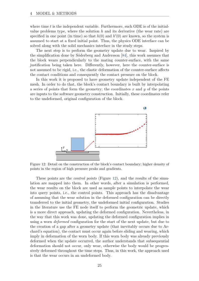
The next step is to perform the geometry update due to wear. Inspired bythe simplification done by Soderberg and Andersson [84], this work assumes thatthe block wears perpendicularly to the mating counter-surface, with the samejustification being taken here. Differently, however, here the counter-surface isnot assumed to be rigid, i.e., the elastic deformation of the counter-surface affectsthe contact conditions and consequently the contact pressure on the block.

In this work it is proposed to have geometry update independent of the FEmesh. In order to do that, the block’s contact boundary is built by interpolatinga series of points that form the geometry; the coordinates x and y of the pointsare inputs to the software geometry construction. Initially, these coordinates referto the undeformed, original configuration of the block.

xy

Figure 12: Detail on the construction of the block’s contact boundary; higher density ofpoints in the region of high pressure peaks and gradients.

These points are the control points (Figure 12), and the results of the simu-lation are mapped into them. In other words, after a simulation is performed,the wear results on the block are used as sample points to interpolate the wearinto query points, i.e., the control points. This approach has the disadvantageof assuming that the wear solution in the deformed configuration can be directlytransferred to the initial geometry, the undeformed initial configuration. Studiesin the literature use the FE node itself to perform the geometric update, whichis a more direct approach, updating the deformed configuration. Nevertheless, inthe way that this work was done, updating the deformed configuration implies inusing a worn deformed configuration for the start of the next update, but due tothe creation of a gap after a geometry update (that inevitably occurs due to Ar-chard’s equation), the contact must occur again before sliding and wearing, whichimply in deformation of the worn body. If this worn body was already previouslydeformed when the update occurred, the author understands that subsequentialdeformation should not occur, only wear, otherwise the body would be progres-sively deformed throughout the time steps. Thus, in this work, the approach usedis that the wear occurs in an undeformed body.

25

4 MODEL & METHODS

In order to better visualize the procedure, consider the following numericalform of Archard’s equation, i.e., the discretized version in time and the use ofimplicit solutions to solve the ODE by the software:

hi+1 = hi + ∆t k pi+1 vs,i+1 (21)

where i is the time step. In COMSOL 5.3, the contact pressure variable used isnamed solid.Tn, and the slip velocity is solid.cnt1.fric1.vslipnorm of the contactpair, calculated by taking into consideration relevant components of the defor-mation gradient projected on the tangent plane, along with the friction and themapped coordinates of the contact pair. The solution of h is then mapped to thecontrol points; from the solution, discrete values of wear are obtained along theboundary, these values are used as sample points to interpolate wear values at thecontrol points, n. Thus, a space discretization is performed in addition to the timediscretization, hn (wear at a control point n) is used to update the coordinate ofthe control points, performing the geometry update. The updated geometry isthen used in the next time step.

In this sense, it is desirable to have several control points, especially in regionswhere high gradients of pressure will occur, such as at the edge of the block, inorder to capture the geometry evolution accurately. The points’ coordinates areread in COMSOL in a interpolation curve operation to build the block’s boundary.It must be highlighted that even though these points are independent of the FEnodes, the FE mesh should still be fine enough to resolve the details to be caughtof the geometry. The FE mesh refinement level throughout the time steps was notchanged, the general appearance is as shown in Figure 11, which was consideredto be a relatively very fine level. One aspect not mentioned yet is that the block’sgeometry contains a fillet at the edge, which not only is in accordance to the actualexperiments, but also conveniently ease the geometry update. Furthermore, inorder to avoid numerical error in the beginning of the simulations, a smoothedstep function was used to gradually increase the wear expression over the first fewtime-steps.

4.3 Long term predictionsEvidently, simulating several time steps to visualize the evolution of contact interms of pressure, wear increment and geometry over a long period of time is com-putationally expensive and impractical. For instance, if one desires to simulate100 cycles for a case in which each cycle is discretized into 20 steps, then 2000simulations would have to be performed. Therefore, it is aimed to use a proce-dure to reduce computational costs while efficiently obtaining results that allowstudying numerous cycles.

The procedures to reduce computational costs are inspired by the approachesdescribed in the previous section, mostly by [58]. Here, the use of an extrapolationfactor is also employed, and so the wear equation is modified

hnj+A,i+1 = hnj,i + A∆tkpni+1vns,i+1 (22)

where A is the extrapolation factor. In addition, we define a cycle j as the move-ment from one extreme to the other and back of the block, i.e., a period. The

26

4 MODEL & METHODS

equation above reflects the approximation that the next “A” cycles will have thesame amount of wear at the same time step “i”. Alternatively, it could be saidthat A artificially increases the wear coefficient. In this sense, it can be said thatEq. (22) simulates real time wear in a material that wears at a A× k wear coeffi-cient, or that it simulates a A cycles of a material that wears at a k wear coefficient.Here, the latter interpretation is used. The parameter A is used within the ODEexpression in COMSOL and controlled through MATLAB.

Furthermore, there is a possibility of using an adaptive extrapolation factor foreach cycle or step, which would possibly make the extrapolation factor differentdepending on which cycle the simulation is currently in. The idea is to maximizethe extrapolation, but maintaining a reliable update; the reliability in this casewould have to be defined by some criterion. The criterion used by Mukras [58] wasthat there should be “smooth pressure distribution” at every update. This leads tothe definition of a critical pressure or critical pressure difference between updates,which in turn defines a scaling factor value (determined by own experimentationin the simulations) which is used to calculate A. The justification is that a smoothcontact surface is consistent with the actual case and a non-smooth surface wouldaffect the FE analysis; in reality, the pressure is generally not perfectly smooth,but the use of an extrapolation factor magnifies any “imperfection”.

In the work of Podra and Anderson [66], they also employed a similar approachto deal with computational costs; in their work they set a “maximum allowedwear increment (...) predefined on the basis of experience and adjusted to as largeas possible by making short simulation test runs.”. Therefore, the extrapolationcriterion definition is a topic of discussion. In this work, the use of an adaptiveextrapolation factor is not employed; constant values of A were chosen based onsimulation tests that would deliberately result in a visible evolution of pressureand wear over a reasonable but short number of update rounds.

The time step ∆t remains fixed when solving the problem, but a second pro-cedure to minimize computational costs is employed: a delay in the geometryupdate by a time ∆tg. The assumption here is that the contact conditions aremaintained for a “∆tg” amount of time, which reduces the amount of geometryupdate, consequently reducing computational costs. It is important to highlightthat ∆t and ∆tg are independent of each other; by increasing ∆t the computa-tional costs would be further reduced, but the solution would be severely affectedby it. Hence, in order to study only the consequences of delaying the geometryupdate, ∆t is maintained fixed at a low value for every simulation.

Differently from [58], in this work what could be called step-update and cycle-update are not fundamentally differently from each other; the geometry-updateoccurs every ∆tg time step, and if this value is chosen in such a way that it has thetime length of a full cycle (2s in our case), the geometry update would occur aftera full cycle, hence a cycle-update. Again, although the geometry update occursat a ∆tg, the wear is solved and accumulated at a ∆t time step.

4.4 Methodology overviewFigure 13 shows the general workflow of the work. Initially, the unworn geometryof the block is prepared by means of a text file containing the coordinates ofthe control points; this file is then used inside COMSOL’s model file to build

27

4 MODEL & METHODS

the block’s contact boundary. Next, the model set-up and the simulations areperformed. The information of contact pressure and wear are stored in MATLABfor post-processing and the geometry update is done according to the desired ∆tgprogrammed in the MATLAB code. Then, the next round is prepared by creatinga new text file with the updated coordinates of the control points that will be usedin the model set-up, once the procedure starts again. The stop criteria refers to anumber of cycles that are desired to be simulated, hence, the procedure works ina for-loop in MATLAB within which the simulations in COMSOL are computed.In fact, the whole procedure is controlled in a MATLAB interface through theLiveLink extension for MATLAB from COMSOL.

FEM simulations

• Contact pressure

• ODE (wear)

Model set-up

• Geometry

• Mat. Prop.

• Physics

• FE mesh

Update procedure

• Updated geometry

Finish

StartInitial

geometry

Post-process

• Verify stop criteria• Prepare next

round set-up xy

Figure 13: Flowchart of wear computation methodology.

28

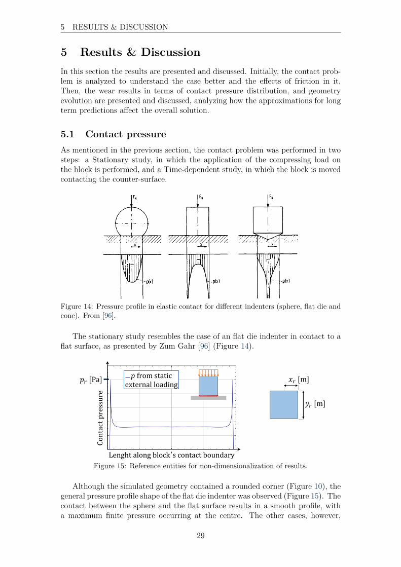
5 RESULTS & DISCUSSION

5 Results & DiscussionIn this section the results are presented and discussed. Initially, the contact prob-lem is analyzed to understand the case better and the effects of friction in it.Then, the wear results in terms of contact pressure distribution, and geometryevolution are presented and discussed, analyzing how the approximations for longterm predictions affect the overall solution.

5.1 Contact pressureAs mentioned in the previous section, the contact problem was performed in twosteps: a Stationary study, in which the application of the compressing load onthe block is performed, and a Time-dependent study, in which the block is movedcontacting the counter-surface.

Figure 14: Pressure profile in elastic contact for different indenters (sphere, flat die andcone). From [96].

The stationary study resembles the case of an flat die indenter in contact to aflat surface, as presented by Zum Gahr [96] (Figure 14).

𝑥𝑟 [m]

𝑦𝑟 [m]

𝑝𝑟 [Pa]

Lenght along block′s contact boundary

𝑝 from staticexternal loading

Contact

pressure

Figure 15: Reference entities for non-dimensionalization of results.

Although the simulated geometry contained a rounded corner (Figure 10), thegeneral pressure profile shape of the flat die indenter was observed (Figure 15). Thecontact between the sphere and the flat surface results in a smooth profile, witha maximum finite pressure occurring at the centre. The other cases, however,

29


results in indeterminate stresses, which is why spherical geometry is preferablewhen calculating elastic contact problems, and also in tribo-experiments.

In order to evaluate the results in a more qualitative manner, the maximumpressure value in the Stationary study (pr) is used as a reference value to normalizethe pressure results; other reference values are the block’s height (yr) and half ofits width (xr). Figure 15 illustrates the quantities.

The effect of friction in the Stationary study is seen in Figure 16; with thepresence of friction (right top), the pressure peaks are higher and the shape ofthe profile does not slightly increase towards the center, as it occurs in the fric-tionless case (left). This can be understood when plotting the x-component of thedisplacement field that is symmetric and occurs due to the Poisson effect and thesymmetric top load: a constraint in the movement of the block’s contact bound-ary is visible in the frictional case. In general, the pressure profile resembles thefrictionless case, because the friction coefficient used is relatively low.

Figure 16: Contact pressure profile (top) normalized by the maximum pressure of thefrictionless case, pr,fric (left) and x-component of the displacement field (bottom); fric-tional case with µ = 0.3 - chosen for visualization purposes only (right).

The inclusion of friction was seen to alter the contact pressure profile also in thetime-dependent study. In the absence of friction, the overall pressure profile wasseen to remain the same as in the static case, unaffected by the movement of theblock. The way friction affects the time-dependent study lies in the configurationof the problem: the displacement of the block is imposed on the top region ofits sides, while the friction causes a tangential force opposing the movement onthe block’s bottom. This configuration would cause the block to tilt towards theleading edge of the movement, which results in an increased contact pressure atthat edge as it contacts the counter-surface. Thus, the pressure profile shifts insuch a way that the pressure peak slightly increase at the leading edge, whileslightly decreasing at the back, as shown in Figure 17.

30


-1 -0.5 0 0.5 1x/x

r

0

0.2

0.4

0.6

0.8

1

1.2

P/P

r

Dynamic pressure field, step 0, cycle 1, dt = 1.00, t = 0.00 s

Figure 17: General normalized dynamic pressure profile on the block’s contact boundaryfor unworn sliding (moving towards the right).

The dynamic pressure profile maintains its shape when the block is movingin the same direction, regardless of the velocity magnitude, which is constantlychanging in this case. When the direction of the movement inverts, the profilesimply inverts with respect to the middle, the highest peak shifting to the leadingedge of the movement.

To better understand the effect of friction on the dynamic pressure, differ-ent values of coefficients of friction were simulated to visualize how the pressurechanges (Figure 18).

μ

Contact

pressure

Leading edge of block′s contact boundary

μ

Contact

pressure

Back edge of block′s contact boundary

ሶ𝑢

Figure 18: Dynamic contact pressure peaks behaviour with regards to coefficient offriction µ changes.

The results confirm the interpretation that the displacement and force config-uration results in a tilting of the block towards the leading edge of the movement;the higher the friction coefficient µ, and thus, the friction force, the more is thetilting, which increases the pressure in the leading edge and decreases it in thetrailing edge of the movement.

5.2 Wear & GeometryOnce the frictional contact problem was solved, the wear and geometry updatecould be performed. The wear is proportional to the slip velocity and the contactpressure; the general initial profile of the dynamic contact pressure was shown

31


in Figure 17, so the general initial profile of wear depth h, or wear increment, issimilar to the one of the dynamic pressure. The slip velocity follows in general thevelocity of the block, which for each time step is essentially constant, increasingand decreasing from the start of the movement until the stop before returning.

The results in this subsection are in terms of: pressure profile evolution, wearincrement evolution, and contact geometry evolution, as the block is worn out.The geometry update time delay (∆tg) was of 2s (one full cycle), 1s, 0.5s, 0.2s,0.1s, 0.05s and the extrapolation factors (A) were of constant fixed values of 500,and 1000.

The left image of the following figures present the wear increment on the block’scontact boundary, normalized by the maximum wear increment of the currentsimulation routine (wi,r). The wear increment yields an updated geometry shownon the right side of the figures, along with the original geometry and a zoomed-inbox on the edge of the block.

5.2.1 Initial simulations

Ideally, we would be able to simulate the least computationally costly case, whichis the longest geometry update delay with the biggest extrapolation. Initially,Figure 19 shows the results using an extrapolation factor of A = 1000 for a coarse∆tg of a full period (2s), which corresponds to sliding the block back and forth,and then updating the geometry. Thus, there is only one geometry update percycle, and each cycle would correspond to 1000 real-life cycles.

-1 -0.5 0 0.5 1x/x

r

0

0.2

0.4

0.6

0.8

1

1.2

wi/w

i,r

Simulation, cycle 1 ( tg = 2 s)

Interpolated at control points

-1 -0.5 0 0.5 1x/x

r

0

0.002

0.004

0.006

0.008

0.01

y/y r

Updated geometry with A = 1000Original geometry

0.94 0.95

x/xr

0

1

2

y/y r

10-3Zoomed-in box

Figure 19: Wear, ∆tg = 2s (“cycle-update”), A = 1000, 1st cycle.

As expected, the wear increment is symmetrical with respect to the block’scontact boundary center; it is noticeable that the high peaks in wear incrementresulted in a relatively deep wear on the block, resembling the wear incrementitself. On the next cycles, the effects of this non-smooth geometry (Figure 20)becomes visible, resulting in a snowball effect, in which neighbouring points willalternate in experiencing high pressure and wear, causing the contact boundaryto become increasingly non-smooth resulting in a “rough” or undulated geometry.Consequently, the emergence of extremely high stress and strain concentrationmay occur, in which other failure mechanisms could occur, besides “breaking” the

32


material model. Finally, the non-smoothness that results from the simulationsof this case start to compromise the successful computation by the software forupcoming cycles.

-1 -0.5 0 0.5 1x/x

r

0

0.2

0.4

0.6

0.8

1

1.2

wi/w

i,r



-1 -0.5 0 0.5 1x/x

r

0

0.002

0.004

0.006

0.008

0.01

y/y r


0.94 0.95

x/xr

1

2

3

y/y r

10-3Zoomed-in box

-1 -0.5 0 0.5 1x/x

r

0

0.2

0.4

0.6

0.8

1

1.2

wi/w

i,r



-1 -0.5 0 0.5 1x/x

r

0

0.002

0.004

0.006

0.008

0.01

y/y r


0.94 0.95

x/xr

0

0.005

0.01

y/y rZoomed-in box

-1 -0.5 0 0.5 1x/x

r

0

0.2

0.4

0.6

0.8

1

1.2

wi/w

i,r



-1 -0.5 0 0.5 1x/x

r

0

0.002

0.004

0.006

0.008

0.01

y/y r


0.94 0.95

x/xr

2

4

6

y/y r

10-3Zoomed-in box

Figure 20: Wear, ∆tg = 2s (“cycle-update”), A = 1000, 2nd, 3rd and 4th cycles.

33


As mentioned in the previous section, similarly to the work of [58], it is assumedthat a smooth contact surface is consistent with the actual case being simulated.Decreasing the extrapolation factor yields different results. Figure 21 present the4th cycle for ∆tg = 2s using A = 500.

-1 -0.5 0 0.5 1x/x

r

0

0.2

0.4

0.6

0.8

1

1.2

wi/w

i,r



-1 -0.5 0 0.5 1x/x

r

0

0.002

0.004

0.006

0.008

0.01

y/y r


0.94 0.95

x/xr

0

2

4

y/y r

10-3Zoomed-in box

Figure 21: Wear, ∆tg = 2s (“cycle-update”), A = 500, 4th cycle.

Using A = 500, the 4th simulated cycle would be the equivalent of simulating2000 cycles. Comparing the 4th cycle with the 2nd cycle of the case with A = 1000,it is possible to notice how the extrapolation can affect the solution. In order toargue which one is more reliable, we recall that Archard’s wear equation assumesa continuous process, thus a simulation with ∆tg tending to zero would approachthe actual case. Although it would be desirable to use a long delay and highextrapolation from the computational costs point of view, the lost in accuracyneeds to be studied.

5.2.2 Finer time steps

If a better time discretization i.e., an increase in time resolution by using smaller∆tg is sufficient to avoid high wear peaks and non-smoothness in the evolvingcontact, then the extrapolation can be maintained. Alternatively, A can be de-creased and the ∆tg may remain coarse. Nevertheless, we wish to approximate thewear process by Archard’s equation, hence a fine step is preferable to approachthe modelling to the equation.

In Figure 22, the first image shows the block at time when it is moving towardsthe right; thus, the wear increment profile resembles the pressure profile scaled bythe slip velocity and it is not symmetrical anymore. On the second row, Figure 22shows the block again at the same moment but on the second cycle, which meansthat the pressure distribution has changed and so has the wear increment; thefigures also shows a moment during the 3rd cycle, in which the block is movingtowards the left and again, the same moment of cycles 1 and 2, but on the 4thcycle, in the last row of Figure 22. Using such fine step, no instabilities such asthe ones seen in the ∆tg = 2s case are visible.

It is important to model the wear increment of all time steps because the slipvelocity is continuously changing, even though the direction of the movement is

34


-1 -0.5 0 0.5 1x/x

r

0

0.2

0.4

0.6

0.8

1

1.2

wi/w

i,r

Simulation, step 8, cycle 1 ( tg = 0.05 s)


-1 -0.5 0 0.5 1x/x

r

0

0.002

0.004

0.006

0.008

0.01

y/y r


0.94 0.950

0.5

110-3

Right edge

-0.95 -0.940

0.5

110-3

Left edge

-1 -0.5 0 0.5 1x/x

r

0

0.2

0.4

0.6

0.8

1

1.2

wi/w

i,r



-1 -0.5 0 0.5 1x/x

r

0

0.002

0.004

0.006

0.008

0.01

y/y r


0.94 0.951

1.2

1.410-3

Right edge

-0.95 -0.941

1.2

1.410-3

Left edge

-1 -0.5 0 0.5 1x/x

r

0

0.2

0.4

0.6

0.8

1

1.2

wi/w

i,r



-1 -0.5 0 0.5 1x/x

r

0

0.002

0.004

0.006

0.008

0.01

y/y r


0.94 0.952

2.2

2.410-3

Right edge

-0.95 -0.942

2.2

2.410-3

Left edge

-1 -0.5 0 0.5 1x/x

r

0

0.2

0.4

0.6

0.8

1

1.2

wi/w

i,r



-1 -0.5 0 0.5 1x/x

r

0

0.002

0.004

0.006

0.008

0.01

y/y r


0.94 0.952.5

2.6

2.710-3

Right edge

-0.95 -0.942.5

2.6

2.710-3

Left edge

Figure 22: Wear, ∆tg = 0.05s, A = 1000, at different moments.

35


constant for half a cycle and then inverts for the other half. However, an approxi-mation could be performed on the slip velocity in the sense to treat it as a scalingfactor of the wear increment, which could further reduce computational costs. Ev-idently, the wear and geometry update is also occurring on the return movement ofthe block. Since the movement starts in one direction, the geometry profile of theedges are different between each other after a few cycles. The simulation startedwith the block moving towards the right direction, thus the left edge wearing isdifferent from the right edge, as can be seen in the zoomed in boxes on the rightside of the figures; the left edge is not only delayed in shape, but it is also less anddifferently worn out compared to the right side..

It was also observed that whenever the movement inverts direction, there isa peak in the wear increment (due to a peak in the pressure because of a newgeometry) on the leading edge. However, this peak is smoothed out during themovement,i.e., the relatively sharp geometry points that yield the peaks, get wornout during sliding. In order to visualize that, the maximum pressure can be trackedduring the simulation and the result of this tracking can be seen in Figure 23.

s0/c1 s20*/c1 s0/c2* s20*/c2 s0/c3* s20*/c3 s0/c4* s20*/c4step/cycle

0

0.3

0.6

0.9

1.2

1.5

Max

imum

P/P

r

Maximum dynamic pressure, tg = 0.05, A = 1000

Figure 23: Maximum dynamic pressure during simulations of 4 cycles; “*” refers toinversion in the direction of motion when associated with a step “s”, or start of a newcycle when associated with a cycle “c”.

The figure shows the smoothing of the pressure during sliding and the rise whenthere is an inversion in the movement. Figure 23 also shows that towards the end,when the maximum pressure is not changing so much anymore, the pressure risesagain - this matter is addressed in the next subsection. At this point, it could bestated that during the first couple of thousands cycles for this case in particular,the contact pressure tends to become more uniform.

The decrease in the pressure peak and tendency for more uniformity in the

36


pressure distribution can be seen in Figures 24. It is expected that regions withhigher pressure will wear more and there will be a tendency for smoothing ofpressure distribution, as long as there is a small ∆tg to capture the the subtlegeometry and pressure changes during the stroke with good accuracy; if the stepis to big, such as in the case previously discussed of ∆tg = 2s, a chain reactionoccurs in the geometry.

-1 -0.5 0 0.5 1x/x

r

0

0.2

0.4

0.6

0.8

1

1.2

P/P

r


-1 -0.5 0 0.5 1x/x

r

0

0.2

0.4

0.6

0.8

1

1.2

P/P

r


Figure 24: Dynamic pressure, ∆tg = 0.05s (named dt on the title), A = 1000, in thebeginning and in the end of the same stroke moving to the right direction.

Another aspect regarding the decrease in the peaks of pressure in Figures 24refers to the contact area; the overall pressure integration along the block’s con-tact boundary is equal to the applied compressive load and it should be constantbecause the load does not change. At first glance, it might seem that the area

37


under the curve of the pressure decreases because of the decrease in the peaks,but the fact is that the contact boundary actually increases, i.e., the contact areaof the block increases as the geometry evolves.

The curve-like “bumps” that develops throughout the cycles at the edges ofthe block due to wear, are an interesting result of the simulations, as it occurs dueto the pressure distribution of the contact, with the geometry naturally evolvingto accommodate the pressure distribution. In order to visualize how the differenttime steps for geometry update affect the geometry, the final geometry after 4cycles can be plotted for different ∆tg; the results are shown in Figure 25.

0.92 0.93 0.94 0.95 0.96x/x

r

2

2.5

3

3.5

4

4.5

5

5.5

6

y/y r

10-3

tg=2s

tg=1s

tg=0.5s

tg=0.2s

tg=0.1s

tg=0.05s

Figure 25: Block’s edge final geometry after 4 cycles with A = 1000.

0.92 0.93 0.94 0.95 0.96x/x

r

1.5

2

2.5

3

3.5

y/y r

10-3

tg=2s

tg=1s

tg=0.5s

tg=0.2s

tg=0.1s

tg=0.05s


38


Figure 26 shows the same results but when using A = 500. From the figures,a few points can be highlighted: firstly, in the A = 1000 we notice that a coarser∆tg than that of 0.05s can be used to result in the same final geometry (∆tg of0.1s and 0.2s resulted in the same); in the A = 500 case, 0.5s is also sufficient.Therefore, it can be said that a convergence is found in the time discretization,but that this convergence depends on the size of the extrapolation; the bigger theextrapolation, the finer should the geometry update time step be. The instabilitiesin the A = 1000 case are revealed sooner than at the last cycle; Figure 27 shows theA = 1000 case after 2 cycles, which would correspond to 4 cycles of the A = 500case; it is seen that the ∆tg of 0.2s, 0.1s, and 0.05s converge to the same geometryand also to the same geometry as A = 500 after 4 cycles for ∆tg of 0.5s, 0.2s,0.1s, and 0.05s. Nevertheless, there is no definitive proof whether further cyclesof either case would reveal instabilities of other ∆tg, but the results obtained heresuggest that it would not.

0.92 0.93 0.94 0.95 0.96x/x

r

1

1.5

2

2.5

3

3.5

y/y r

10-3

tg=2s

tg=1s

tg=0.5s

tg=0.2s

tg=0.1s

tg=0.05s


5.2.3 Full-scale simulation

In order to evaluate the capacity of the model, and attempt to study long-termtests in order to test the statement that the contact pressure tends to become moreuniform, a 20 hour test-equivalent simulation was performed by using A = 4000and ∆tg = 0.05s, chosen based on the results presented above. The conditionsare the same as in the previous results, stated in Table 2. Using A = 4000, 9cycles would be the equivalent to a 20 h experiment, resulting in 36000 cycles. Itis important to highlight that a smaller extrapolation with proportionally morecycles could also be performed. For academic purposes the combination of 4000and 9 for the extrapolation and number of cycles, respectively, was chosen in thissection.

In Figure 28, similar to Figure 23, the maximum pressure is tracked. Becauseof the higher value of extrapolation, A, a less smooth accommodation of pressure

39


s0/c1 s20*/c1 s0/c2* s20*/c2 s0/c3* s20*/c3 s0/c4* s20*/c4step/cycle

0.3

0.6

0.9

1.2

1.5

1.8

Max

imum

P/P

r


Figure 28: Maximum dynamic pressure during simulations of first 4 cycles with A =4000; “*” refers to inversion in the direction of motion when associated with a step “s”,or start of a new cycle when associated with a cycle “c”.

is visible. At the middle of cycle 1 towards its end, the same rise in the maximumpressure observed at the mid-end of cycle 4 of Figure 23 is seen again. It could beargued that such rise occurs due to the very nature of the problem, in which oncethe pressure distribution smoothed to a certain level, further wear of the geometryresults again in sharp geometry leading to a peak in pressure.

s0/c5* s0/c6* s0/c7* s0/c8* s0/c9*step/cycle

0.3

0.6

0.9

1.2

1.5

1.8

Max

imum

P/P

r


Figure 29: Maximum dynamic pressure during simulations of 4th to 9th cycles withA = 4000.

40


Figure 29 shows the continuation of the 9 cycles routine; at first glance it mightseem chaotic, but the general trend of uniforming pressure distribution is observed.The various sudden peaks in pressure are the result of an excessive extrapolationfactor, which at certain steps yields out sharp geometry and consequently highpressures. At these steps, the wear increment shape becomes non-smooth, whichwould characterize instabilities and hence not consistent with the actual case beingsimulated. However, the non-smooth steps do not start a “snowball effect” in thesense of making the next steps increasingly unstable, as occurred in the initialstudied cases with ∆tg = 2s.

An example of such case is for example during the cycle 6, shown in Figure 30.In this case, the peak in the wear increment comes from a pressure peak whichoccurs due to a sharp geometry of the current step. It is safe to say that ifthe extrapolation were not so big in the previous step, the evolution of contactand pressure would occur more smoothly and such peak would not be present.As written previously, the steps that follow do not result in an ever increasinglyunstable profile, hence the routine can be further analyzed.

-1 -0.5 0 0.5 1x/x

r

0

0.2

0.4

0.6

0.8

1

1.2

wi/w

i,r



-1 -0.5 0 0.5 1x/x

r

0

0.02

0.04

0.06

0.08

0.1

y/y r


0.95 0.96 0.970.0145

0.015

0.0155

Right edge

-0.97 -0.96 -0.950.014

0.015

0.016

Left edge

Figure 30: Step showing non-smooth wear increment during the 6th cycle with A = 4000.

Other steps which with non-smooth wear increment have similar instabilities inthe sense that they occur at the edge region of the contact. They are a consequenceof the extrapolation, the time and space discretization, and the methodology ofgeometry update. Despite the numerical limitation, the general trend that can beseen from Figure 29 is as stated previously, i.e., the maximum pressure tends tovanish and the pressure distribution become more uniform as the block slides inthe same direction and peaks again when the movement inverts direction.

Figure 31 shows the wear increment and geometry profile at selected momentsof the full case simulation. In all, it is possible to simulate such long periodswith the chosen parameters of this subsection with an overall stability, althoughsmaller extrapolation or even smaller ∆tg would result in smoother results, but atthe expense of more computational costs.

41


-1 -0.5 0 0.5 1x/x

r

0

0.2

0.4

0.6

0.8

1

1.2w

i/wi,r



-1 -0.5 0 0.5 1x/x

r

0

0.02

0.04

0.06

0.08

0.1

y/y r


0.95 0.96 0.976

6.2

6.410-3

Right edge

-0.97 -0.96 -0.955

6

710-3

Left edge

-1 -0.5 0 0.5 1x/x

r

0

0.2

0.4

0.6

0.8

1

1.2

wi/w

i,r



-1 -0.5 0 0.5 1x/x

r

0

0.02

0.04

0.06

0.08

0.1

y/y r


0.95 0.96 0.970.0115

0.012

0.0125

Right edge

-0.97 -0.96 -0.950.011

0.0115

0.012

Left edge

-1 -0.5 0 0.5 1x/x

r

0

0.2

0.4

0.6

0.8

1

1.2

wi/w

i,r



-1 -0.5 0 0.5 1x/x

r

0

0.02

0.04

0.06

0.08

0.1

y/y r


0.95 0.96 0.970.015

0.0155

0.016

Right edge

-0.97 -0.96 -0.950.014

0.015

0.016

Left edge

-1 -0.5 0 0.5 1x/x

r

0

0.2

0.4

0.6

0.8

1

1.2

wi/w

i,r



-1 -0.5 0 0.5 1x/x

r

0

0.02

0.04

0.06

0.08

0.1

y/y r


0.95 0.96 0.970.0208

0.021

0.0212

Right edge

-0.97 -0.96 -0.950.0205

0.021

Left edge

Figure 31: Wear, ∆tg = 0.05s, A = 4000, at different moments.

42

6 CONCLUSIONS & FUTURE WORKS

6 Conclusions & Future worksIn this work, the development of a numerical model and method to predict contactpressure, wear and contact geometry evolution of a linearly reciprocating block incontact to a flat plane was performed. The development of the model problememployed assumptions in both the physics and the material to the specific casethat need to be taken into consideration when critically analyzing the results.The wear computation methodology was inspired by the literature review andalso makes use of assumptions discussed in the text.

Regarding solid mechanics, it was observed in the structural analysis that thecontact pressure and the slip velocity have noticeable high peaks and gradientstowards the edges of the block, due to the physics of the structural configuration ofcontact and the geometries involved. Consequently, the wear reaches high valuesand gradients in these regions as well. The inherent discrete nature of the FEMmakes it a challenge to capture the gradients at the edge of the contact pair.However, the space discretization with the “control points” allowed an interestinguse of the simulation results, besides a straightforward geometry update procedure.

The emergence of a non-smooth geometry is intuitively not expected in a realcase; not only due to the non-existence of the limitations of the multiple discretiza-tion in the simulation model, but also because of other phenomena taking place,such as transfer-film formation or temperature related events. Furthermore, theresults are also limited to the equations it is solving, i.e., Archard’s wear equation,which doesn’t consider, e.g., the generation of wear particles.

The lack of consideration of other phenomena in the modelling may limit theperspective of relating the simulations of this work to events observed in experi-ments, at least at this initial stage. Despite of that, results have shown that thereis a dynamic process occurring during sliding and wearing, which have implicationswith regards to the way the wear coefficient is empirically determined, namely theassumption of constant and uniform pressure in the contact region at all time.

In all, the goal of developing the model and methodology was achieved, result-ing in a tool that can be used to study contact pressure, wear, and geometry of alinearly reciprocating block on flat plane. In terms of recommendations of futureworks, a few topics could be studied: the implementation of more physics, e.g.,heat transfer or transfer film; the computation of wear also on the counter-surfaceand see how the interface contact evolves. Also, different wear models or modifi-cation of the wear equation could be performed by applying pressure and slidingvelocity dependent wear coefficient, or by adding some smoothing that would acton the pressure peaks and gradients by use of a PDE instead of ODE. Further-more, the inclusion of third-body or wear particles could be interesting. Finally,3D modelling could provide more information by studying the influence of theblock’s corners and 3D stress fields.

43

References[1] Ahmed Abdelbary. Wear of polymers and composites. Woodhead Publishing,

2015.[2] Tatsuhiko Aizawa, Thananan Akhadejdamrong, and Atsushi Mitsuo. “Self-

lubrication of nitride ceramic coating by the chlorine ion implantation”. In:Surface and Coatings Technology 177 (2004), pp. 573–581.

[3] Joel Andersson. “Modelling of wear and tribofilm growth”. PhD thesis. Luleatekniska universitet, 2012.

[4] Joel Andersson, Andreas Almqvist, and Roland Larsson. “Numerical simu-lation of a wear experiment”. In: Wear 271.11-12 (2011), pp. 2947–2952.

[5] Ivan Argatov and Wilson Tato. “Asymptotic modeling of reciprocating slid-ing wear–comparison with finite-element simulations”. In: European Journalof Mechanics-A/Solids 34 (2012), pp. 1–11.

[6] Shyam Bahadur. “The development of transfer layers and their role in poly-mer tribology”. In: Wear 245.1 (2000), pp. 92–99.

[7] Kim Berglund and Yijun Shi. “Friction and Wear of Self-Lubricating Mate-rials for Hydropower Applications under Different Lubricating Conditions”.In: Lubricants 5.3 (2017), p. 24.

[8] Sanghita Bhattacharya. “Predictive finite element modeling of artificial cer-vical discs in a ligamentous functional spinal unit”. PhD thesis. 2011.

[9] Peter J Blau. “How common is the steady-state? The implications of weartransitions for materials selection and design”. In: Wear 332 (2015), pp. 1120–1128.

[10] Peter J Blau. “On the nature of running-in”. In: Tribology international38.11-12 (2005), pp. 1007–1012.

[11] C Boher et al. “A wear model based on cumulative cyclic plastic straining”.In: Wear 267.5-8 (2009), pp. 1087–1094.

[12] BRIAN J Briscoe and SK Sinha. “Wear of polymers”. In: Proceedings of theInstitution of Mechanical Engineers, Part J: Journal of Engineering Tribol-ogy 216.6 (2002), pp. 401–413.

[13] DL Burris and WG Sawyer. “Addressing practical challenges of low frictioncoefficient measurements”. In: Tribology letters 35.1 (2009), pp. 17–23.

[14] A Cantizano, A Carnicero, and Giorgio Zavarise. “Numerical simulation ofwear-mechanism maps”. In: Computational materials science 25.1-2 (2002),pp. 54–60.

[15] Federico J Cavalieri, Fernando Zenklusen, and Alberto Cardona. “Determi-nation of wear in internal combustion engine valves using the finite elementmethod and experimental tests”. In: Mechanism and machine theory 104(2016), pp. 81–99.

[16] Chang Chongyi, Wang Chengguo, and Jin Ying. “Study on numerical methodto predict wheel/rail profile evolution due to wear”. In: Wear 269.3-4 (2010),pp. 167–173.

[17] COMSOL. COMSOL Multiphysics - Reference Manual. Version: COMSOL5.3. 2017.

[18] Liang Deng et al. “Numerical study of contact conditions in press hardeningfor tool wear simulation”. In: International Journal of Material Forming 10.5(2017), pp. 717–727.

[19] DJ Dickrell, DB Dooner, and WG Sawyer. “The evolution of geometry for awearing circular cam: analytical and computer simulation with comparisonto experiment”. In: Journal of Tribology 125.1 (2003), pp. 187–192.

[20] Vamshidhar Done et al. “Semi analytical fretting wear simulation includingwear debris”. In: Tribology International 109 (2017), pp. 1–9.

[21] J Dyson and W Hirst. “The true contact area between solids”. In: Proceedingsof the Physical Society. Section B 67.4 (1954), p. 309.

[22] Tom Fleischman. Researchers simulate wear of materials as they rub to-gether. [Online]. [Accessed 26 May 2018]. Available from: http://news.cornell.edu/stories/2016/06/researchers-simulate-wear-materials-they-rub-together. 2016.

[23] Anders Flodin and Soren Andersson. “A simplified model for wear predictionin helical gears”. In: Wear 249.3-4 (2001), pp. 285–292.

[24] FJ Franklin, I Widiyarta, and A Kapoor. “Computer simulation of wear androlling contact fatigue”. In: Wear 251.1-12 (2001), pp. 949–955.

[25] Walter Frei. Meshing Considerations for Linear Static Problems - COM-SOL Blog. [Online]. [Accessed 02 June 2018]. Available from: https : / /www . comsol . com / blogs / meshing - considerations - linear - static -problems/. 2013.

[26] Klaus Friedrich and Alois K Schlarb. Tribology of polymeric nanocomposites:friction and wear of bulk materials and coatings. Vol. 55. Elsevier, 2011.

[27] Yuan-cheng Fung and Pin Tong. Classical and computational solid mechan-ics. World Scientific, 2001.

[28] Arash Golchin, Gregory F Simmons, and Sergei B Glavatskih. “Break-awayfriction of PTFE materials in lubricated conditions”. In: Tribology Interna-tional 48 (2012), pp. 54–62.

[29] C Gonzalez et al. “Numerical analysis of pin on disc tests on Al–Li/SiCcomposites”. In: Wear 259.1-6 (2005), pp. 609–612.

[30] JA Greenwood, H Minshall, and David Tabor. “Hysteresis losses in rollingand sliding friction”. In: Proc. R. Soc. Lond. A 259.1299 (1961), pp. 480–507.

[31] JA Greenwood and JB Pl Williamson. “Contact of nominally flat surfaces”.In: Proc. R. Soc. Lond. A. Vol. 295. 1442. The Royal Society. 1966, pp. 300–319.

[32] Liangjin Gui et al. “A simulation method of thermo-mechanical and tribo-logical coupled analysis in dry sliding systems”. In: Tribology International103 (2016), pp. 121–131.

http://news.cornell.edu/stories/2016/06/researchers-simulate-wear-materials-they-rub-together



https://www.comsol.com/blogs/meshing-considerations-linear-static-problems/



[33] Bernard J Hamrock, Steven R Schmid, and Bo O Jacobson. Fundamentalsof fluid film lubrication. CRC press, 2004.

[34] V Hegadekatte et al. “Multi time scale simulations for wear prediction inmicro-gears”. In: Wear 268.1-2 (2010), pp. 316–324.

[35] Vishwanath Hegadekatte, N Huber, and O Kraft. “Finite element basedsimulation of dry sliding wear”. In: Modelling and Simulation in MaterialsScience and Engineering 13.1 (2004), p. 57.

[36] Seiichro Hironaka. “Boundary lubrication and lubricants”. In: Three bondtechnical news 9 (1984), pp. 1–8.

[37] Anders Hugnell and Soeren Andersson. “Simulating follower wear in a cam—followercontact”. In: Wear 179.1-2 (1994), pp. 101–107.

[38] Anders B-J Hugnell, Stefan Bjoerklund, and Soeren Andersson. “Simulationof the mild wear in a cam-follower contact with follower rotation”. In: Wear199.2 (1996), pp. 202–210.

[39] Ian Hutchings and Philip Shipway. Tribology: friction and wear of engineer-ing materials. Butterworth-Heinemann, 2017.

[40] Peter Ireman, Anders Klarbring, and Niclas Stromberg. “Finite element algo-rithms for thermoelastic wear problems”. In: European Journal of Mechanics-A/Solids 21.3 (2002), pp. 423–440.

[41] Gao Jintang. “Tribochemical effects in formation of polymer transfer film”.In: Wear 245.1 (2000), pp. 100–106.

[42] L Johansson. “Numerical simulation of contact pressure evolution in fret-ting”. In: Journal of tribology 116.2 (1994), pp. 247–254.

[43] Kenneth Langstreth Johnson and Kenneth Langstreth Johnson. Contact me-chanics. Cambridge university press, 1987.

[44] Mitjan Kalin. “Influence of flash temperatures on the tribological behaviourin low-speed sliding: a review”. In: Materials Science and Engineering: A374.1 (2004), pp. 390–397.

[45] Nam Ho Kim et al. “Finite element analysis and experiments of metal/metalwear in oscillatory contacts”. In: Wear 258.11-12 (2005), pp. 1787–1793.

[46] PL Ko et al. “Finite element modelling of crack growth and wear particleformation in sliding contact”. In: Wear 251.1-12 (2001), pp. 1265–1278.

[47] Laszlo Konya and Karoly Varadi. “Wear simulation of a polymer–steel slid-ing pair considering temperature-and time-dependent material properties”.In: Tribology and Interface Engineering Series. Vol. 55. Elsevier, 2008, pp. 130–145.

[48] JK Lancaster. “Abrasive wear of polymers”. In: Wear 14.4 (1969), pp. 223–239.

[49] KA Laux et al. “The influence of surface properties on sliding contact tem-perature and friction for polyetheretherketone (PEEK)”. In: Polymer 103(2016), pp. 397–404.

[50] Jakub Lengiewicz and Stanis law Stupkiewicz. “Efficient model of evolutionof wear in quasi-steady-state sliding contacts”. In: Wear 303.1-2 (2013),pp. 611–621.

[51] PBC Linear. Simplicity Technology from PBC Linear. [Online]. [Accessed 09November 2017]. Available from: https://www.youtube.com/watch?v=aD224gX39G0. 2011.

[52] FJ Martınez, MA Jimenez, and MA Martınez. “Application of wear mod-elling methodology to the design of a lift car installation by means of finiteelement simulation”. In: Meccanica 49.2 (2014), pp. 393–411.

[53] FJ Martinez et al. “Finite element implementation and validation of wearmodelling in sliding polymer–metal contacts”. In: Wear 284 (2012), pp. 52–64.

[54] Marcia Marie Maru and Deniol K Tanaka. “Consideration of stribeck dia-gram parameters in the investigation on wear and friction behavior in lubri-cated sliding”. In: Journal of the Brazilian Society of Mechanical Sciencesand Engineering 29.1 (2007), pp. 55–62.

[55] IR McColl, J Ding, and SB Leen. “Finite element simulation and experi-mental validation of fretting wear”. In: Wear 256.11-12 (2004), pp. 1114–1127.

[56] HC Meng and KC Ludema. “Wear models and predictive equations: theirform and content”. In: Wear 181 (1995), pp. 443–457.

[57] JF Molinari et al. “Finite-element modeling of dry sliding wear in metals”.In: Engineering Computations 18.3/4 (2001), pp. 592–610.

[58] Saad Mukras et al. “Numerical integration schemes and parallel computationfor wear prediction using finite element method”. In: Wear 266.7-8 (2009),pp. 822–831.

[59] Nikolai Myshkin et al. “Contact mechanics and tribology of polymer com-posites”. In: Journal of Applied Polymer Science 131.3 (2014).

[60] NK Myshkin, MI Petrokovets, and AV Kovalev. “Tribology of polymers: ad-hesion, friction, wear, and mass-transfer”. In: Tribology International 38.11(2006), pp. 910–921.

[61] Rudolf Novak and Tomas Polcar. “Tribological analysis of thin films by pin-on-disc: Evaluation of friction and wear measurement uncertainty”. In: Tri-bology International 74 (2014), pp. 154–163.

[62] Mona Oqvist. “Numerical simulations of mild wear using updated geometrywith different step size approaches”. In: Wear 249.1-2 (2001), pp. 6–11.

[63] I Paczelt and Z Mroz. “On optimal contact shapes generated by wear”. In:International Journal for Numerical Methods in Engineering 63.9 (2005),pp. 1250–1287.

[64] Michael Peigney. “Simulating wear under cyclic loading by a minimizationapproach”. In: International journal of solids and structures 41.24-25 (2004),pp. 6783–6799.

https://www.youtube.com/watch?v=aD224gX39G0

https://www.youtube.com/watch?v=aD224gX39G0

[65] George Plint. Guidance Notes on Friction. Tech. rep. [Online]. [Accessed 13January 2018]. Available from: http://www.phoenix-tribology.com/wp-content/uploads/guidance/Guidance-Laws-of-Friction.pdf. 2005.

[66] Priit Podra and Soren Andersson. “Finite element analysis wear simulationof a conical spinning contact considering surface topography”. In: Wear 224.1(1999), pp. 13–21.

[67] Priit Podra and Soren Andersson. “Simulating sliding wear with finite ele-ment method”. In: Tribology international 32.2 (1999), pp. 71–81.

[68] Priit Podra and Soren Andersson. “Wear simulation with the Winkler surfacemodel”. In: Wear 207.1-2 (1997), pp. 79–85.

[69] E. Rabinowicz. Friction and Wear of Materials. A Wiley-Interscience pub-lication. Wiley, 1995. isbn: 9780471830849. url: https://books.google.se/books?id=1uVSAAAAMAAJ.

[70] Fernando Ramırez et al. “A new approach for time-space wear modelingapplied to machining tool wear”. In: Wear 390 (2017), pp. 125–134.

[71] Jeremy J Rawlinson et al. “Wear simulation of the ProDisc-L disc replace-ment using adaptive finite element analysis”. In: (2007).

[72] Ali Rezaei et al. “Adaptive finite element simulation of wear evolution inradial sliding bearings”. In: Wear 296.1-2 (2012), pp. 660–671.

[73] Ali Rezaei et al. “Experimental study and numerical simulation of the large-scale testing of polymeric composite journal bearings: two-dimensional mod-eling and validation”. In: Tribology letters 37.2 (2010), pp. 261–272.

[74] DA Rigney. “The roles of hardness in the sliding behavior of materials”. In:Wear 175.1-2 (1994), pp. 63–69.

[75] Maria Rodiouchkina et al. “Material Characterization and Influence of Slid-ing Speed and Pressure on Friction and Wear Behavior of Self-LubricatingBearing Materials for Hydropower Applications”. In: Lubricants 6.2 (2018).

[76] E Santner and H Czichos. “Tribology of polymers”. In: Tribology Interna-tional 22.2 (1989), pp. 103–109.

[77] W Gregory Sawyer. “Wear predictions for a simple-cam including the cou-pled evolution of wear and load”. In: Tribology & Lubrication Technology57.9 (2001), p. 31.

[78] Tony L Schmitz et al. “The difficulty of measuring low friction: uncertaintyanalysis for friction coefficient measurements”. In: Journal of Tribology 127.3(2005), pp. 673–678.

[79] GK Sfantos and MH Aliabadi. “Wear simulation using an incremental slidingboundary element method”. In: Wear 260.9-10 (2006), pp. 1119–1128.

[80] KJ Sharif, HP Evans, and RW Snidle. “Prediction of the wear pattern inworm gears”. In: Wear 261.5-6 (2006), pp. 666–673.

[81] Jintao Shen. “Self-lubricating Polymer Composites: Tribology and Inter-face”. PhD thesis. 2015.

http://www.phoenix-tribology.com/wp-content/uploads/guidance/Guidance-Laws-of-Friction.pdf

http://www.phoenix-tribology.com/wp-content/uploads/guidance/Guidance-Laws-of-Friction.pdf

https://books.google.se/books?id=1uVSAAAAMAAJ

https://books.google.se/books?id=1uVSAAAAMAAJ

[82] Xuejin Shen et al. “Numerical simulation of sliding wear for self-lubricatingspherical plain bearings”. In: Journal of materials research and technology1.1 (2012), pp. 8–12.

[83] VA Smurugov et al. “On PTFE transfer and thermoactivation mechanismof wear”. In: Wear 158.1-2 (1992), pp. 61–69.

[84] Anders Soderberg and Soren Andersson. “Simulation of wear and contactpressure distribution at the pad-to-rotor interface in a disc brake usinggeneral purpose finite element analysis software”. In: Wear 267.12 (2009),pp. 2243–2251.

[85] Christer Spiegelberg and Soren Andersson. “Simulation of friction and wearin the contact between the valve bridge and rocker arm pad in a cam mech-anism”. In: Wear 261.1 (2006), pp. 58–67.

[86] Gwidon Stachowiak and Andrew W Batchelor. Engineering tribology. Butterworth-Heinemann, 2013.

[87] Henrik Sonnerlind. What Is Geometric Nonlinearity? [Online]. [Accessed 05November 2017]. Available from: https://www.comsol.com/blogs/what-is-geometric-nonlinearity/. 2015.

[88] David Tabor. “Friction—the present state of our understanding”. In: J. Lubr.Technol 103.2 (1981), pp. 169–179.

[89] Thordon. THORPLAS-BLUE BEARINGS FOR INDUSTRIAL APPLICA-TIONS. [Online]. [Accessed 19 September 2017]. Available from: http://thordonbearings.com/system/documents/documents/192/original/ThorPlas_Blue_Industrial_brochure.pdf?1381422411. nA.

[90] Thordon. ThorPlas® Bearings Engineering Manual Version: TP2006.1. [On-line]. [Accessed 19 September 2017]. Available from: http://thordonbearings.com/system/documents/documents/36/original/ThorPlas_Engineering_ManualA4.pdf?1278591962. nA.

[91] Tribonet. Archard Wear Equation. [Online]. [Accessed 04 December 2017].Available from: http://www.tribonet.org/wiki/archard-wear-equation/.2017.

[92] Anton Van Beek. “Advanced engineering design”. In: Tu Delft (2006), pp. 87–136.

[93] Peter Wriggers and Tod A Laursen. Computational contact mechanics. Vol. 2.Springer, 2006.

[94] Wenyi Yan, Noel P O’Dowd, and Esteban P Busso. “Numerical study ofsliding wear caused by a loaded pin on a rotating disc”. In: Journal of theMechanics and Physics of Solids 50.3 (2002), pp. 449–470.

[95] Dong-Ya Zhang et al. “Tribological Properties of Self-Lubricating Polymer–Steel Laminated Composites”. In: Tribology Transactions 56.6 (2013), pp. 908–918.

[96] K-H Zum Gahr. Microstructure and wear of materials. Vol. 10. Elsevier,1987.

https://www.comsol.com/blogs/what-is-geometric-nonlinearity/

https://www.comsol.com/blogs/what-is-geometric-nonlinearity/

http://thordonbearings.com/system/documents/documents/192/original/ThorPlas_Blue_Industrial_brochure.pdf?1381422411



http://thordonbearings.com/system/documents/documents/36/original/ThorPlas_Engineering_ManualA4.pdf?1278591962



http://www.tribonet.org/wiki/archard-wear-equation/

simulations of contact mechanics and wear of linearly

Documents