simulation: transactions of the society for modeling and
TRANSCRIPT

Simulation
Simulation: Transactions of the Society for
Modeling and Simulation International
89(8) 935–963
� 2013 The Society for Modeling and
Simulation International
DOI: 10.1177/0037549713484077
sim.sagepub.com
A new framework for thesimulation of equation-based modelswith variable structure
Dirk Zimmer
AbstractMany modern models contain changes that affect the structure of their underlying equation system, e.g. the breaking ofmechanical devices or the switching of ideal diodes. The modeling and simulation of such systems in current equation-based languages frequently poses serious difficulties. In order to improve the handling of variable-structure systems, anew modeling language has been designed for research purposes. It is called Sol and it caters to the special demands ofvariable-structure systems while still representing a general modeling language. This language is processed by a newtranslation scheme that handles the differential-algebraic equations in a highly dynamic fashion. In this way, almost arbi-trary structural changes can be processed. In order to minimize the computational effort, each change is processed aslocally as possible, preserving the existing computational structure as much as possible. Given this methodology, trulyobject-oriented modeling and simulation of variable-structure systems is made possible. The corresponding process ofmodeling and simulation is illustrated by two examples from different domains.
Keywordsvariable-structure systems, equation-based modeling, differential-algebraic equations, index reduction
1. Introduction
Modern modeling methodologies in the field of physical
systems are increasingly based on equation-based model-
ing languages. Such languages have a declarative character
and are based on differential-algebraic equations (DAEs).
Furthermore, they feature various object-oriented con-
structs that enable a proper organization of knowledge. In
this way, models can be built up hierarchically and com-
posed out of submodels belonging to various domains.
Nowadays, the most prominent equation-based lan-
guage is Modelica.1,2 It was designed in the late 1990s by
an international standardization committee. A number of
companies have meanwhile adopted the Modelica technol-
ogy. Large-scale system models, e.g. describing the
dynamics of cars, consisting of several hundreds of thou-
sands of lines of code have been encoded in this language.
These models have proven to be as run-time efficient as
the best manually encoded models of the past.
Nevertheless, there are also other languages that feature
equation-based modeling. For instance VHDL-AMS3 or
gPROMS4 are being used in industry. Smaller languages
such as Chi5,6 serve academic interests.
Unfortunately, many of these languages share a com-
mon deficiency. They suppose a fixed computational
structure of the resulting model and, hence, the support of
variable-structure systems is very limited. However, many
contemporary models contain structural changes at simula-
tion run-time. The motivations for these models are
manifold:
• The structural change is caused by ideal switching
processes. Classic examples are ideal diodes in
electric circuits and rigid mechanical elements that
can break apart.• The model features a variable number of variables:
this issue typically concerns social or traffic simu-
lations that feature a variable number of agents or
entities, respectively.• The variability in structure is to be used for reasons
of efficiency: a bent beam should be modeled in
German Aerospace Center, Institute of System Dynamics and Control,
Weßling-Oberpfaffenhofen, Germany
Corresponding author:
Dirk Zimmer, German Aerospace Center, Institute of System Dynamics
and Control, Munchner Strasse 20, D-82234 Weßling-Oberpfaffenhofen,
Germany.
Email: [email protected]

more detail at the point of the buckling and more
sparsely elsewhere.• The variability in structure results from user inter-
action: when the user is allowed to create or con-
nect certain components at run time, this usually
results in a structural change.
Evidently, the collective term variable-structure systems is
very general and can be applied to various modeling para-
digms such as agent-simulations or finite-element meshes.
In this paper, we focus on the modeling within object-
oriented equation-based languages for multi-physics sys-
tems (e.g. Modelica1,2 or gPROMS4). In order to obtain a
more precise picture for the particular problems in this
domain, let us look at a suitable example: the trebuchet.
1.1. The trebuchet
The trebuchet is an old catapult weapon developed in the
middle ages. It is known for its long range and its high pre-
cision. Figure 1 depicts a trebuchet and presents its func-
tionality. It is a seemingly simple system but its simulation
involves severe structural changes on a higher-index sys-
tem (see Sections 4 and 5). Technically, the system can be
described within planar mechanics and it is a double pen-
dulum propelling a projectile in a sling. The rope of the
sling is released on a predetermined angle γ when the pro-
jectile is about to overtake the lever arm. Furthermore, the
following assumptions hold true for the modeling:
• All mechanics are planar. The positional states of
any object are therefore restricted to x, y, and the
orientation angle ’.• All elements are rigid. Also the sling is non-elastic.• The rope of the sling is ideal and weightless. It
exhibits an inelastic impulse when being stretched
to maximum length.• The revolute joint of the counterweight is limited to
a certain angle β (in order to prevent too heavy
back-swinging after the projectile’s release). It also
exhibits an inelastic impulse when reaching its limit.
Whereas these idealizations simplify the parameterization
of the model to a great extent, they pose serious difficulties
for a typical simulation environment of an equation-based
language. This ideal modeling leads to various structural
changes that occur during the simulation of the system. At
t = 0:5 s, one of these changes is recognizable in the trajec-
tory of the projectile (Figure 2) as discrete change of the
first time derivative.
1.2. Modeling the trebuchet
The most direct approach is to model the system as a
whole. In modern object-oriented modeling environments
0 0.5 1 1.5
-15
-5
5
15
25
t[s]
x[m
]
0 0.5 1 1.50
10
20
30
4040
t[s]
y[m
]
-20 0 20 400
10
20
30
40
x[m]
y[m
]
Figure 2. Trajectory of the projectile.
Figure 1. Functionality of a trebuchet.
936 Simulation: Transactions of the Society for Modeling and Simulation International 89(8)

such an approach is still possible but certainly unfavored.
The resulting model would be highly complex and none of
its parts could be properly reused. For another mechanical
system, the modeling would have to be redone from
scratch again.
Instead, the system is composed out of individual com-
ponents that form a model library and interact with each
other by a common interface. For this example, the follow-
ing components suffice:
• one fixation component (F);• four fixed translations (T0, T1, T2, T3);• one revolute joint (R1);• one limited revolute joint (R2);• two bodies with mass and inertia (B1, B2);• one ideal rope with a body attached to it (TB).
The assembly of the system from these components is rep-
resented by the model diagram of Figure 3. In the next
step, we have to assign a correct set of equations to each
component. Let us look at the equations for the simple
revolute joint:
’2 =’1 +’R1
x2 = x1
y2 = y1
fx, 1 + fx, 2 = 0
fy, 1 + fy, 2 = 0
t1 + t2 = 0
t2 = 0
These equations relate the interface variables of the com-
ponent. These are the variables that represent the position:
x, y, and the angle ’. The second set describes the force
and torque fx, fy, and t. The interface variables are indexed
by subscripts 1 or 2 according to which of the two inter-
faces they belong to.
The angle ’R1 of the revolute is not the sole variable of
interest; also its velocity ωR1 and acceleration αR1 can be
helpful variables for the simulation of mechanical systems.
Hence the set of equations is extended by the following
two differential equations:
ωR1 = _’R1
αR1 = _ωR1
The trebuchet contains not only a simple revolute joint,
but also a version with a limited range that is similar in its
functionality to an elbow. The corresponding model can be
described by two major modes: free or fixated. The mode
free is equivalent to a normal revolute joint whereas the
model equals a fixed orientation in the fixated mode. The
transition between these modes is triggered when the angle
of the revolute exceeds a predetermined limit β. Since this
transition causes a discrete change in velocity, it involves an
inelastic impulse on the rigidly connected components.
Furthermore impulses from other components (such as for
instance the ideal rope) need to be handled as well in this
component. The different modes and their transitions are
presented in the graph of Figure 4, where the continuous-
time modes are depicted as round boxes and the rectangular
boxes denote intermediate modes that cause discrete (imme-
diate) changes in the value of variables.
m=100
B1
m=10e3
B2
a b
r={-10,0}
T3a b
r={2,5,0}
T1
F
r={0
,0}
ab
R1
ab
r={-2
,-1.5
}
T2
m=15
TB
a b
R2
ab
r={0
,8}
T0
Figure 3. Model diagram of the trebuchet.
Zimmer 937

The modeling of variable-structure systems by different
modes cannot be achieved by a pure equation-based mod-
eling in a convenient manner. The modeling of different
modes and their transition needs to be considered as well.
Furthermore events need to be described that trigger the
transition. In addition, equations for the impulse behavior
of the system need to be formulated. In order to be concise,
we omit these aspects here and focus only on the structural
change between the continuous-time modes. Here, each
mode has its separate set of equations.
The difference between these two modes is presented in
Table 1. The variables ’R2, ωR2, αR2 cease to exist in the
fixated mode and, therefore, there are three fewer equa-
tions in the corresponding set of equations. Five of the
remaining six equations are shared by both modes and,
thus, the structural change concerns only a subset of the
total modeling equations.
We see that we can represent this structural change by
a simple modification in a set of DAEs. Thus, it may ini-
tially seem surprising that such an easy model cannot be
realized within current equation-based languages for phys-
ical systems. Although the structural change may seem tri-
vial for the individual component, it is severe for the
complete model of the trebuchet. It changes the number of
continuous-time states and leads to different algebraic
equations systems. The index reduction of the DAE sys-
tems requires the automatic differentiation of certain
model equations (see Section 5). Depending on the
continuous-time mode of the limited revolute, different
equations need to be differentiated.
The situation is even more complicated, when we con-
sider that the limited revolute joint is not the only compo-
nent of the trebuchet that causes structural changes. The
component for the torn body introduces another three inde-
pendent continuous-time modes:
1. The body is at rest as long as the rope has not been
stretched.
2. The body represents a pendulum as long as the
release angle γ has not been reached.
3. The body is free.
For each of these modes, different variables are used to
describe the positional state of the body. In the first mode,
the position is constant and the model contains no state
variables. In the second mode, the angle and angular velo-
city define the positional states, whereas the body is free
in the last mode and consequently defines the maximum
of six state variables.
There are three components that define all state vari-
ables of the system. These are the limited and non-limited
version of the revolute joint and the component for the torn
body. The combination of modes from these three compo-
nents forms the modes of the complete system. Figure 5
displays that in total there occur five modes where only
two of them are equivalent. Furthermore, there are two
intermediate modes for the inelastic impulses that are rep-
resented by the vertical lines spanning over the affected
components. Here the velocities ωR1 and ωR2 are disabled
as state variables. Hence, the number of continuous-time
state variables in total varies from 2 to 10.
Even for such a simple mechanical system as the trebu-
chet, it is difficult for a modeler to foresee all of these
combinations of modes. In order to enable a truly object-
oriented modeling, it is therefore an essential prerequisite
that the corresponding simulation environment supports
the automatic derivation of these mode combinations and
can generate the correct set of equations. If the modeler
would be forced to model all modes and their transitions
at the top level, the modeling would become extremely
laborious. Furthermore, the resulting solution would not
be generic, and its parts would hardly be reusable.
1.3. Related work
Obviously, the modeling and simulation (M&S) of
variable-structure systems is a challenging task. Even a
simple mechanical system as the trebuchet poses a number
of difficulties for a general M&S framework. Hence, such
a system cannot be modeled in Modelica. There are, how-
ever, alternative modeling languages that are better geared
towards variable-structure systems.
Table 1. Transition form free to fixated mode.
Free Fixated
’2 = ’1 +’R2 ’2 = ’1 +bx2 = x1 x2 = x1y2 = y1 y2 = y1fx,1 + fx,2 = 0 fx,1 + fx,2 = 0fy,1 + fy,2 = 0 fy,1 + fy,2 = 0t1 + t2 = 0 t1 + t2 = 0t2 = 0oR2 = _’R2
aR2v = _oR2
angle
exceeds
limit
externalimpulse fixatedfree
inelastic impulse
torque becomes
negative
contact signal
triggers
Figure 4. Mode-transition graph of the limited revolute.
938 Simulation: Transactions of the Society for Modeling and Simulation International 89(8)

The project MOSILAB7 created an extension to the
Modelica language that enables the formulation of struc-
tural changes by means of state charts. In this way, differ-
ent parts of the model can be activated or deactivated. To
enable a formulation with the aid of state charts, it is nec-
essary that the complete system is decomposable into a
finite set of modes. Thus, MOSILAB represents a feasible
solution only when the structural changes are modeled on
the top level. If, however, these changes emerge from sin-
gle components, MOSILAB becomes insufficient. The tre-
buchet represents a suitable example for this. Its
implementation in MOSILAB would require that all of its
modes are described on a global level. Although theoreti-
cal possible, it would be difficult to achieve. The advan-
tage of MOSILAB is that it is a true compiler and
generates efficient simulation code.
More promising approaches with respect to a true
object-oriented modeling style have been achieved in the
field of hybrid bondgraphs. In this methodology, structural
changes are modeled by ideal switches that connect or dis-
connect components of the bondgraph. This suffices for
most structural changes in physical systems as long as the
number of components is known beforehand. It is insuffi-
cient when components need to be instantiated or removed
during simulation time. Within the field of hybrid bond-
graphs, the projects HYBRSIM8 and the work of
Roychoudhury et al.9 are notable. In case of HYBRSIM,
the bondgraph is simulated by an interpreter that is able to
handle up to index-two systems. The work of
Roychoudhury et al.9 favors a translation to a causal block
diagram that is being simulated in Matlab Simulink. The
approach that tries to preserve the previous causal struc-
ture of the bondgraph by applying incremental update
algorithms is interesting. It is similar to the approach
described in this paper, but less general as it is restricted
to bondgraphs.
A recent project is represented by Hydra.10–12 This is a
modeling language that originates from functional pro-
gramming languages such as Yampa and has been devel-
oped at the University of Nottingham. Hydra is based on
the paradigm of functional hybrid modeling. This makes
it a powerful language. In principle, it is possible to state
arbitrary equation systems with Hydra and to formulate
arbitrary changes. Also new elements can be generated
at run-time. Practically, the simulation engine has not
yet been able to demonstrate support higher-index sys-
tems to a sufficient extent. The way Hydra is processed
is rather unique in the field of M&S. Hydra features a
just-in-time compilation. At each structural change, the
model is completely recompiled in order to enable a fast
evaluation of the system. This approach makes Hydra
interesting with respect to this paper since it represents a
complementary approach to the incremental algorithms
presented here.
Unfortunately, none of these tools demonstrates the
ability to model and simulate the trebuchet in a true object-
oriented style. Therefore, we decided to develop a new
framework called Sol. There are two major objectives
behind this project:
1. The language Sol shall enable a true object-
oriented modeling style where physical compo-
nents containing structural changes can be
assembled componentwise. This part of the project
is published elsewhere.13–15
2. The computational framework of Sol shall investi-
gate how the structural changes in the set of DAEs
can be handled by incremental algorithms includ-
ing higher-index problems. To this end, classic
methods for index reduction for static systems are
revisited and integrated in a more dynamic frame-
work. This is the main content of this paper.
Time
0.0 0.25 0.5 0.75 1.0 1.25 1.5 1.75 2.0
Resting: { }Torn Body Pendulum: {φTB, ωTB} Free: {xTB, yTB, φTB, vTB,x, vTB,y, ωTB}
Free: {φR2, ωR2}Limited
RevoluteFree: {φR2, ωR2} Fixated: {}
Free: {φR2, ωR2}
Continuoustime states
4 6 10 8 10
82
{ φR1, ωR1}Main
Revolute{ φR1, ωR1}{ φR1, ωR1}
...at impulse
Figure 5. Structural changes of the trebuchet.
Zimmer 939

Hence, we proceed by presenting the computational frame-
work of Sol. Its final capability and performance is then
presented in Section 6.
1.4. The Sol framework
Figure 6 depicts the typical processing scheme that is
shared by many equation-based languages such as
Modelica and involves multiple stages of compilation. It
starts with the parsing of the model files and ends with the
generation of code that serves simulation or optimization
tasks. In this way, a quasi-static computational structure of
the model is imposed that prevents the simulation of many
classes of structural changes.
In order to enable the handling of variable-structure sys-
tems, these processing stages need to be rearranged so that
the set of equations can arbitrarily change over run-time.
To this end, we provide a new simulation framework
called Solsim. Figure 7 depicts the new processing scheme.
Since Solsim represents an interpreter, the code-generation
is replaced by a direct evaluation. This evaluation stage is
used for performing time integration but it may also trigger
events that lead to structural changes in succession. To
manage these structural changes, new components have to
be reinstantiated and flattened. Furthermore, the causality
of the whole system may need to be updated. Thus, these
three stages that represented a sequence in the classic pro-
cessing scheme form now a loop.
The most central part in the processing scheme of Sol
is the dynamic DAE processing that replaces the former
causalization stage. In this stage, the flattened set of equa-
tions is transformed into a set of computations that suits
numeric ordinary differential equation (ODE) solvers. It is
especially this stage that makes equation-based modeling
languages so powerful. The modeler is relieved of the
tedious task that consists of the computational realization
of his models. It enables also that models can be stated in
a declarative manner and are generally applicable. To this
end, a great number of elaborate algorithms have been
developed for the static case. For many commercial sys-
tems such as Dymola16 most of these algorithms repre-
sents the heart of their compiler and partly because of this,
their major parts are mostly still under non-disclosure.
Even the static causalization of DAEs is far from being
trivial. Handling arbitrary changes in a system of DAEs
represents a major challenge. The exchange of single equa-
tion may enforce a complete rebuild of the whole computa-
tional form. In most of the cases, however, a partial update
of the system suffices. In this paper, we present a
framework with its algorithms and methods for the
dynamic case that can track changes in an efficient
manner.
To this end, it is necessary that we look in detail at the
processing of DAEs. Hence, the next four sections present
the theoretic fundamentals of the Solsim simulation envi-
ronment and are not directly application oriented. Section
2 introduces the terminology and presents the basic entities
of the applied data structures. Section 3 then explains the
handling of index-zero systems and the main principles of
our processing algorithm. Systems that contain algebraic
loops are discussed in Section 4 whereas higher-index sys-
tems are discussed in Section 5. The final section revisits
the trebuchet catapult and presents another application
example of the Sol framework.
The implementation of Solsim represents a prototype
simulator that shall demonstrate the feasibility of the sug-
gested methodology and the functionality of the proposed
algorithms. The program itself is a command-line program
implemented in C++ . The resulting simulation data is
dumped to a file. Since the program is a proof of concept
and not a mature software tool, the software has not been
published but interested readers may contact the author.
2. Dynamic DAE processing2.1. Fundamentals
This section defines fundamental notions and terminology
used in the following. In order to ease the understanding
Parsing
Instantiationand Flattening
Preprocessing
Dynamic DAE Processing
Evaluation
Time
Integration
Event
Handling
Figure 7. Dynamic processing of Sol.
ParsingInstantiation
and FlatteningPreprocessing Causalization
CodeGeneration
Figure 6. Typical processing of equation-based languages.
940 Simulation: Transactions of the Society for Modeling and Simulation International 89(8)

of the abstract definitions, we provide a small and simple
example for illustrative purposes. Figure 8 presents an
electric circuit with a capacitor. It contains a multi-switch
that triggers various structural changes.
Listing 1 presents the corresponding Sol model for this
circuit.
1 model Circuit
2 implementation:
3 static Real R;
4 static Real C;
5 static Real i;
6 static Real u_C;
7 static Real u_R;
8 static Real u_Sw;
9 static Integer mode;
10 C = 0.01;
11 R = 100;
12 u_C + u_R + u_Sw = 0;
13 u_R = R*i;
14 i = C*der(x=u_C);
15 mode << f(x=time);
16 if mode == 0 then
17 u_Sw = 10;
18 else if mode == 1 then
19 static Real freq;
20 freq = 5;
21 u_Sw = 10* cos(x=freq*(time -5));
22 else if mode == 2 then
23 i = -0.2;
24 else then
25 static Real R2;
26 R2 = 1000;
27 u_Sw = R2*i;
28 end if;
29 end Circuit;
Listing 1. Flat Sol model of an electric circuit with multi-switch.
In order to present a concise and traceable example, the
Sol model here refrains from any object-oriented con-
structs that are provided by the language: the model has
already been manually flattened and contains no hierarchic
structure. The precise syntax and semantics of Sol are out-
lined by Zimmer.13 However, the presented example can
be briefly explained: it consists of the declaration of vari-
ables (e.g. static Real R;) and relations. Relationsare either non-causal equations (e.g. u_R = R*i) orcausal assignments. For example, line 15 states that thevalue of the integer variable mode is assigned (withfixed causality) by the result of the function f whoseinput parameter x equals time. Please note that the syn-tax for function calls in Sol (e.g. f(x = time))
requires an explicit binding between formal and actualparameters. Some of the variables and equations arestated within conditional branches (if . then .else .). The activation and deactivation of thesebranches yield structural changes.
The Sol model of Listing 1 represents a set of DAEs. In
general, such a system can be described in the implicit
DAE form:
0=F( _xp(t), xp(t), u(t), t)
The target of the dynamic DAE processor (DDP) is to
achieve a transformation of F into the state space form f
that is directly applicable for the purpose of numerical
ODE solution
_x(t)= f (x(t), u(t), t)
The level of difficulty of this transformation is described
by the perturbation index.17,18 The transformation itself is
consequently denoted as index reduction. This classic
DAE perspective is essential but not sufficient.
Unfortunately, many models contain more than just DAEs.
In particular, variable-structure models are hybrid models
that involve both continuous and discrete parts. It is there-
fore too simplistic to look at the problem from the
continuous-time perspective of DAEs only. We need a
more general approach.
We give a few remarks regarding the notation of the
following sections: lowercase characters are applied to
individual entities such as variables, tuples, relations, etc.
Capital letters are applied to sets or certain functions.
With respect to relations, when we refer to a specific
relation of Listing 1, we use italic line numbers as indices.
For instance r13 represents u_R = R*i.
2.1.1. Relations. We define a system s as a pair (2-tuple)
that consist in a set of active relations R, a set of active
variable identifiers V :
s= (R,V )
Mostly, the variables identifiers point to real numbered
values, but there are no restrictions applied. The variables
identified in V may be of any basic or compound type. A
relation may represent a non-causal equation or a causal
assignment of the model. A relation represents typically an
equation of the model or a causal assignment. Three func-
tions can be applied on a relation r in order to determine
its dependences on variables in V .
The system s often represent just the current mode of
the system. For a variable structure system, this means that
the sets R and V are subject to change during time.
The function D(r) returns a set of all variables identi-
fiers that the relation r depends on: its dependences. These
variables need to be evaluated first before the relation r
Zimmer 941

can be processed. The function U (r) returns the set of vari-
ables identifiers that may be determined by the relation: its
potential unknowns. Furthermore, the presence in the set R
of a relation may depend on a certain set of variables iden-
tifiers that is represented by L(r). Such dependences are
denoted as logic dependences.
For illustration, let us take a look at three relations of
our example above.
• r12 represents u_C + u_R + u_Sw = 0.
This relation is a simple, non-causal equation between
three variables: D(r12)= fu_C, u_R, u_Swg. Since theequation does not stipulate the causality, all of the vari-ables are potential unknowns: U (r12)=D(r12). Thereare no logic dependences involved: L(r12)=1.
• r15 represents mode << f(x=time).
This relation is a causal assignment and contains two vari-
ables of different type: D(r15)= fmode, timeg. Theassignment predetermines the causality, so there is onlyone potential unknown: U (r15)= fmodeg. Again, thereare no logic dependences involved: L(r15)=1.
• r17 represents u_Sw = 10.
Since this equation is stated within a branch statement, its
presence in the active set of relations R is related to
the variable mode. This is a logic dependence L(r17)=
{modeg. Consequently: D(r17)= fu_Sw, modeg andU (r17)=D(r17)\L(r17).
2.1.2. Causality graph. In order to transform the system s into
a form that is useful for computational purposes, we need to
assign a causality c to each of the relations in R. The causal-
ity determines which of the occurring variables an equation
should be solved for. Hence, a causality c is defined to be a
pair of a relation and one of its potential unknowns:
c= (r, u)with u∈U (r)
The set of causalities C has to represent a bijective map-
ping between subsets of V and R. Relations that have a
causality assigned are being denoted as causalized, other
relations as non-causalized. The sets of variables V , rela-
tions R and causalities C can be composed to a tuple:
(R,V ,C)
This tuple can be represented as a causality graph. This is
a directed acyclic graph (DAG) G(V ,E) where the ver-
tices represent the relations of the system VG =R. A rela-
tion r1 that determines one of its unknowns u∈U (r1) has
outgoing edges to all of those relations r2 that are depen-
dent on u. In this way the causality graph depicts the com-
putational flow:
EG = (r1, r2)jr1 6¼ r2 ^ ((r1, u)∈C ^ u∈Dr2 )f g
R=100
R
R=1000
R2
G
C=0.01
C
V=10
+
U0
+-
I=0.2
clock
t
-
Figure 8. Diagram of an electric circuit with multi-switch.
942 Simulation: Transactions of the Society for Modeling and Simulation International 89(8)
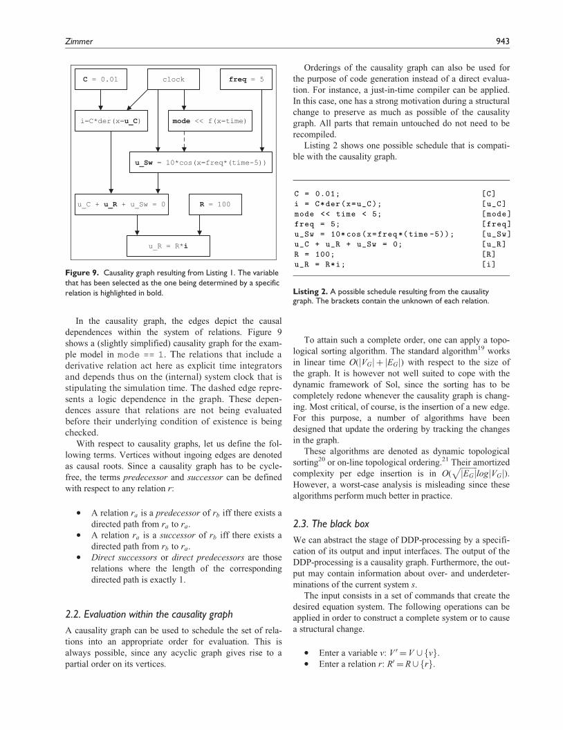
In the causality graph, the edges depict the causal
dependences within the system of relations. Figure 9
shows a (slightly simplified) causality graph for the exam-
ple model in mode == 1. The relations that include aderivative relation act here as explicit time integratorsand depends thus on the (internal) system clock that isstipulating the simulation time. The dashed edge repre-sents a logic dependence in the graph. These depen-dences assure that relations are not being evaluatedbefore their underlying condition of existence is beingchecked.
With respect to causality graphs, let us define the fol-
lowing terms. Vertices without ingoing edges are denoted
as causal roots. Since a causality graph has to be cycle-
free, the terms predecessor and successor can be defined
with respect to any relation r:
• A relation ra is a predecessor of rb iff there exists a
directed path from ra to ra.• A relation ra is a successor of rb iff there exists a
directed path from rb to ra.• Direct successors or direct predecessors are those
relations where the length of the corresponding
directed path is exactly 1.
2.2. Evaluation within the causality graph
A causality graph can be used to schedule the set of rela-
tions into an appropriate order for evaluation. This is
always possible, since any acyclic graph gives rise to a
partial order on its vertices.
Orderings of the causality graph can also be used for
the purpose of code generation instead of a direct evalua-
tion. For instance, a just-in-time compiler can be applied.
In this case, one has a strong motivation during a structural
change to preserve as much as possible of the causality
graph. All parts that remain untouched do not need to be
recompiled.
Listing 2 shows one possible schedule that is compati-
ble with the causality graph.
C = 0.01; [C]
i = C*der(x=u_C); [u_C]
mode << time < 5; [mode]
freq = 5; [freq]
u_Sw = 10* cos(x=freq*(time -5)); [u_Sw]
u_C + u_R + u_Sw = 0; [u_R]
R = 100; [R]
u_R = R*i; [i]
Listing 2. A possible schedule resulting from the causalitygraph. The brackets contain the unknown of each relation.
To attain such a complete order, one can apply a topo-
logical sorting algorithm. The standard algorithm19 works
in linear time O(jVGj+ jEGj) with respect to the size of
the graph. It is however not well suited to cope with the
dynamic framework of Sol, since the sorting has to be
completely redone whenever the causality graph is chang-
ing. Most critical, of course, is the insertion of a new edge.
For this purpose, a number of algorithms have been
designed that update the ordering by tracking the changes
in the graph.
These algorithms are denoted as dynamic topological
sorting20 or on-line topological ordering.21 Their amortized
complexity per edge insertion is in O(ffiffiffiffiffiffiffiffiffijEGj
plogjVGj).
However, a worst-case analysis is misleading since these
algorithms perform much better in practice.
2.3. The black box
We can abstract the stage of DDP-processing by a specifi-
cation of its output and input interfaces. The output of the
DDP-processing is a causality graph. Furthermore, the out-
put may contain information about over- and underdeter-
minations of the current system s.
The input consists in a set of commands that create the
desired equation system. The following operations can be
applied in order to construct a complete system or to cause
a structural change.
• Enter a variable v: V 0=V ∪ fvg.• Enter a relation r: R0=R∪ frg.
C = 0.01 clock freq = 5
i=C*der(x=u_C) mode << f(x=time)
u_Sw = 10*cos(x=freq*(time-5))
u_C + u_R + u_Sw = 0 R = 100
u_R = R*i
Figure 9. Causality graph resulting from Listing 1. The variablethat has been selected as the one being determined by a specificrelation is highlighted in bold.
Zimmer 943

• Remove a relation r: R0=R\frg.• Remove a variable v: V 0=V\fvg.
This list of operations provides us with an abstraction
layer that enables us to interpret the DDP processor as a
black box. For convenience, we will use the symmetric dif-
ference _s between two system s1 and s2 to describe a struc-
tural change:
_s= f _R, _Vg= (s1\s2)∪ (s2\s1)
Hence, _R contains all relations that are being removed
or added and _V contains all variables that are being
removed or added.
3. Index-zero systems3.1. Demands on a dynamic framework
In the dynamic framework, variables and their corresponding
relations can be added and removed at all times. To avoid
overdetermination, old relations are removed from the system
before they are replaced by new relations. Thus, intermediate
underdetermination must be tolerated. Overdetermination, in
contrast, shall be detected immediately.
Both processes, removing and adding, cause changes
in the corresponding causality graph. The DDP tracks
each of these changes in an efficient manner. However, a
worst-case analysis is not a good performance measure,
since the replacement of a single relation may cause the
recausalization of the whole system. In the worst case,
the smartest thing to do is a recausalization of the com-
plete system. Obviously, this is not a good approach in
general.
In order to be efficient, the DDP should preserve the
existing causality graph as much as possible, so that the
causality graph and the corresponding ordering must not
be changed more often and more widely than necessary. It
is the goal to prevent unnecessary changes in the causality
graph and restrict modifications to those parts only that are
affected by the change.
3.2. Forward causalization
Forward causalization is the base algorithm for causaliza-
tion. It assigns a causality c to a non-causalized relation r.
It represents a simple straightforward algorithm, a variant
of topological sorting that is part of many similar algo-
rithms, for instance the Tarjan algorithm.22
This algorithm can be implemented as a graph algo-
rithm. In the dynamic framework, this procedure is exe-
cuted whenever a new relation is added. It calls itself
recursively and potentially updates all successors of the
relation. For Algorithm 1 and all following algorithms, the
sets R (relations), V (variables), and C (causalizations) are
available as global variables.
Input: a relation rOutput: causality c = (u, r)D′ is the set of direct predecessors of r.It is initially empty: D′ := ∅;for all v ∈ D(r) do
if v is determined,i.e. (v, r′) ∈ C with r′ �= r thenD′ := D′ ∪ {v};
end
endAttempt to causalize r, given D′;if causalization was successful then
Retrieve its unknown u;Assign and enter the causality: C := C ∪ {(u, r)};for all relations ra succeeding r with u ∈ D(r) do
apply forward causaliz. recursively for r = ra;end
end
Algorithm 1. Forward causalization.
The actual causalization of a single relation r is not described
here, but later on in Section 3.6. However, the causalization of r
depends always on its knowns D0⊆D(r) and on its kind. There are
two kinds of relations in Sol: causal relations (assignments) and
non-causal relations (equations).
For instance, a causality can be assigned for non-causal
relations, if all but one element of D(r)\L(r) are deter-
mined by other relations. Further kinds of relations are
presented in Sections 4 and 5 that have their own charac-
teristics and serve special purposes.
If the computational flow of a system can be expressed
in the form of a simple causality graph, forward causaliza-
tion is fully sufficient. Forward causalization will fail, if
the system is under- or overdetermined. It will fail as well,
if the system contains algebraic loops. This case is dis-
cussed in Section 4.
Another reason for failure is that not all relations can
be solved for all of its unknowns. For instance, a relation r
like sin(x=phi) = a can only be solved for a but notfor phi. However, this demands no modification of thepresented algorithms. The inability to solve for phi issimply expressed by the set of unknowns: U (r)= {a}whereas D(r)= {a, phi}. If the causal structure of thesystem demands for instance the inversion of the sinefunction, an artificial algebraic loop will result by theapplication of the methods in Section 4.
3.3. Potential causality
The reverse process to forward causalization would be for-
ward decausalization. It consists in removals of causalities in
C. One could implement this in a similar way. This process
would then be executed, each time a relation is removed.
However, this represents an overeager approach, since each
944 Simulation: Transactions of the Society for Modeling and Simulation International 89(8)

structural change might involve a temporal underdetermina-
tion of the system. If this temporal underdetermination
affects a causal root of the system, forward decausalization
would remove many or even all causalities from the system,
just to see them potentially reinstated a few steps later.
In order to avoid such overhasty reconfigurations of the
causality graph, we introduce the concept of potential cau-
salization. This means that, once a causalization has been
assigned to a relation, the relation will not lose this causal-
ity again. This is even the case if some of its ‘‘knowns’’
are not determined anymore; instead the relation is being
marked as potentially causalized.
Whenever a relation r with its causality c(u, r) is
removed, the following steps are executed:
1. The causality c= (u, r) is removed: C : =C\f(u, r)g.
2. Attempt to causalize all direct successors rsucc of r.
3. If the attempt fails, the relation rsucc remains poten-
tially causalized.
4. Remove r: R : =R\frg.
For instance, let us consider the switch from mode 1
to mode 0 in the example of Listing 1:
_s= (fr17, r20, r21g, ffreqg). First, the two relations r20and r21 are removed. The relation r12, representing u_C+ u_R + u_Sw = 0 is dependent on r21 and is there-fore causalized again. It remains potentially causalized.
Now the relation r17 is added to the system. It is directly
causalized by the subsequent forward causalization and deter-
mines u_Sw again. As a consequence, r12 releases itspotential state, and the causality graph is once more com-plete. This specific structural change could be handledwith minimal effort: no unnecessary decausalization hadto be performed.
3.4. Causality conflicts and residuals
Potentially causalized relations only replace their former
causality, if they are being contradicted by other relations.
To illustrate this, let us suppose that we are now switching
from mode 0 to mode 2 in the example model. The corre-
sponding change is _s= (fr17, r23g,1).
This change does yield a causality conflict. After
removing the relation r17, r12 remains potentially causa-
lized. The newly added relation r23 cannot be causalized,
since its only potential unknown i is already determined
by the relations r13, representing u_R = R*i. The relationr23 is overdetermined.
To cope with this conflict, r23 generates a residual ρ
and U (r23) expands in correspondence. The residual ρ rep-
resents the difference between the two sides of the equa-
tion. It should of course be zero. Also the causality
c= (ρ, r23) is generated. Residuals are globally collected
in the set O. Whenever the process of forward causalization
stops and O 6¼1, the residuals are thrown. Throwing resi-
duals means that sources of overdetermination are looked
up and assigned to the residual. Potentially causalized rela-
tions represent one possible source of overdetermination.
The lookup for sources includes all predecessors of the
relations that determine a residual. Whenever a potentially
causalized relation is assigned to a residual, all causalities
of the corresponding predecessor paths are first marked
and finally collectively removed. Algorithm 2 presents one
possible implementation. It detects all sources in a recur-
sive depth-first traversal and marks them and all of their
predecessors while tracking back the traversal path. Finally
all marked relations are decasualized.
In the given example, the relation r12 is potentially causa-
lized and assigned to the residual as source of overdetermina-
tion. The relations r13, r23 are those predecessors of the
residual that are successors of r12 and are marked by adding
them to the set P. Their causalization is collectively removed.
By applying forward causalization on the members of
P, the relation r23 will be causalized again and remove its
residual, since it determines the variable i. The conflict has
been resolved, and all relations can be causalized. In gen-
eral, the lookup for the potential path can be achieved by
the recursive Algorithm 2. The algorithm is called for the
relations that have thrown the residuals in O.The presented processing scheme represents the general
approach of the DDP.
1. Overdetermined relations generate a residual. This
residual is thrown into the set O.2. When forward causalization stops, all residuals in
O are examined.
3. The examination looks for a source of overdeter-
mination in all predecessors of the corresponding
overdetermined relation.
4. If a source is found, the conflict is resolved by
means appropriate to the type of the source.
Input: a relation rOutput: global set P of members of the potential pathInitially (non-recursive), P := ∅;Recursive section:for each direct predecessors ra of r do
if ra is potentially causalized thenP := P ∪ {r, ra};
elsecall this algorithm recursively for r = ra;if ra ∈ P then
P := P ∪ {r};end
end
endFinally (non-recursive) begin
for each r′ ∈ P doremove causality: C := C \ {( , r′)};
endfor each (non-causalized) r′ ∈ P do
perform forward causalization on r′;end
end
Algorithm 2: Potential path detection and removal.
Zimmer 945

The last point in the list makes a very general statement:
‘‘by means appropriate’’. For this particular problem, over-
determination was caused by potentially causalized rela-
tions. The appropriate procedure was to recausalize the
path that has been potentially causalized.
We shall see in the next sections that there are other
sources of overdetermination as well. They will call for
other means in order to resolve the conflict, but the out-
lined processing scheme proves to be of general value.
3.5 Avoiding cyclic subgraphs
The causality graph is defined to be an acyclic graph. If it
is constructed solely by the process of forward causaliza-
tion, it is guaranteed to be acyclic. Yet having potentially
causalized relations in the graph, this statement does not
hold true anymore. We need to ensure that it remains
acyclic.
A cycle may occur whenever a potentially causalized
relation rp gets causalized again. If this occurs, one has to
verify that none of the predecessors of rp is also a succes-
sor of rp.
If the verification fails, the graph contains a cyclic sub-
graph with at least one potentially causalized relation. The
cyclic subgraph is defined to be the union of all directed
paths starting and ending at rp. The causalities of all rela-
tions belonging to this cyclic subgraph have to be
removed. An algorithm for this purpose would be similar
to Algorithm 2.
Their causality will not necessarily get reinstated by
further forward causalization. The system may contain
an algebraic loop. An example for this is the switch from
mode 0 to mode 3 with _s= (fr17, r26, r27g, fR2g). Againr12 becomes potentially causalized. After adding r26the relation r27 is added and is causalized to u_Sw.This would reinstate the causality of r12, but r12, r13,and r27 form a cyclic subgraph. All their causalitieswill be removed.
Forward causalization will not be able to complete the
causalization anymore. However, the system is not under-
determined. It contains an algebraic loop. For this particu-
lar example, this means that a linear equation system needs
to be solved, in order to compute the voltage divider that is
created by the two series-connected resistors. Section 4
will discuss how such systems and more complicated ones
can be handled in a dynamic manner.
3.6. States of relations
We have not yet described how the causalization of a sin-
gle relation works. We know from the previous sections
that the dynamic framework expects that the relations can
be in different states. By name, these are:
• non-causalized: the relation has no causality c
assigned to it;• potentially causalized: the relation retains its former
causality although it is currently not valid anymore;• causalized: the relation determines one of its poten-
tial unknowns;• causalized with residual: the relation is overdeter-
mined and determines a residual.
The dynamic framework may remove the causality of any
relation at any time, as this happens with the potentially
causalized paths that lead to a residual. Otherwise, the rela-
tion may change its state by any attempt of causalization
during forward causalization.
The transition between the states is best described by a
state-transition diagram. It is dependent on the type of the
relation. Sol offers mainly two types: equations, these are
non-causal relations; and transmissions, these are causal
relations.
For instance, equations in Sol represent non-causal rela-
tions r and fulfill the condition U (r)=D(r)\L(r). In order
to be causalized, they require that all but one variable of
U (r) are causalized. Figure 10 depicts the corresponding
behavior of non-causal relations. The labels at the edges
denote the events that trigger a state transition. If none of
these conditions is fulfilled, the relation rests in its current
state. The states not-causalized and causalized may serve
as intermediate states.
3.7. Asymptotic complexity
The first objective is to show that the proposed algorithms
terminate. The second objective is to present an upper
bound for the complexity of the algorithms. Since these
algorithms are graph algorithms, it is the most natural
choice to use the number of vertices jVGj and the number
of edges jEGj as definition for the problem size. Often
however, one is simply referring to the system size n. For
all meaningful applications of Sol, it is a safe assumption
to state that n= jVGj and O(jEGj)=O(jVGj). The latter
assumption implies the sparsity of the equation system.
Let us start with forward causalization. This algo-
rithm will terminate simply because it can only increase
the number of variables that are being determined by a
relation. This requires that the individual relations do
not lose their causality by the determination of arbitrary
variables. This requirement is fulfilled for both kinds of
relations.
The causality graph is generated by forward causaliza-
tion. The state transitions for causal and non-causal rela-
tions imply that a relation can be causalized if it is a
causal root or if all of its predecessors in the causality
graph have been causalized. Since forward causalization
will process all relations at least once, all causal roots will
946 Simulation: Transactions of the Society for Modeling and Simulation International 89(8)

be causalized. Since the algorithms processes all direct
successors of a causalized relation, also the non-root rela-
tions will be causalized. Forward causalization fails if
there are algebraic loops or equations that cannot be cau-
salized as desired because of non-linearities.
The algorithmic complexity of forward causalization is,
not surprisingly, the same as for the topological ordering.
Each relation is processed at least once. If a relation has been
causalized, all its outgoing edges are being traversed. If all
relations have been causalized, all edges will have been tra-
versed. Since each relation is causalized only once, the total
complexity of the algorithm is in O(jVGj+ jEGj) or O(n).
Here O(jVGj+ jEGj) is also the upper bound for any
traversal of successors or predecessors in the causality
graph. Hence, the throwing of residuals requires
O(jOj(jVGj+ jEGj)), since each residual requires a traver-
sal of its predecessors in order to find its sources of over-
determination. It is possible to reduce the upper bound to
O((jVGj+ jEGj)) by a collective traversal in the graph, but
that does require an additional, non-constant cost in mem-
ory per vertex in the graph.
Another traversal of successors or predecessors is
needed to assure that the causality graph remains cycle
free. Hence, the recausalization of potentially causalized
equations requires costs in O(jVGj+ jEGj). Mostly, how-
ever, this operation is much cheaper. The ordering that is
required for the evaluation of the causality graph may be
used for a quick test if the graph is cycle-free. In our
implementation, we use priority numbers, and in this way,
cycle-freeness can be quickly affirmed.
Finally, we have to show that any arbitrary structural
change is handled correctly. Since such a change may
cause an alternating sequence of forward causalizations
and causality removals, it is not evident that the algorithm
will terminate. Therefore, it is of importance that all resi-
duals are collectively thrown and the corresponding
potential paths are collectively removed. This includes the
potential cycles.
By doing so, one ensures that the subsequent forward
causalization is processed on a subgraph without poten-
tially causalized relations. If there remain residuals or new
residuals have been created, there will be no source of
overdetermination for them, and the residuals indicate an
overdetermination of the complete system.
In this way, four steps are sufficient to correctly handle
any structural change that leads to a regular system of
index-zero.
1. Equations that are being replaced are removed. Their
direct successors remain potentially causalized.
2. New equations are added to the system. Forward
causalization is applied to them. Potential causali-
zations may get re-established.
3. Residuals are thrown (if any). Potentially causa-
lized paths are reset.
4. Forward causalization is executed once more on
the reset part.
It is possible to implement all these steps in
O(jVGj+ jEGj). This guarantees that the handling of struc-
tural changes has the same algorithmic complexity as a
complete rebuild of the system. This would be optimal since
the worst-case scenario would cause a complete rebuild.
The following list describes those structural changes in
index-zero systems that can be handled more efficiently.
• Structural changes that add components to the exist-
ing computational flow.• Structural changes that replace components but
retain the computational flow.• Arbitrary structural changes that depend only on a
small set of variables.
notcausalized
potentiallycausalized
causalized
in residual form
• >(n-1) variables determined
• external reset<(n-1) variables determined
external reset
>(n-1) variables determined
n variables determined• < n variables determined
• external reset
Figure 10. State transitions of non-causal relations. The cardinality of U(r) is denoted as n.
Zimmer 947

4. Index-one systems4.1. Algebraic loops
The target of the DDP is to transform the system s= (R,V )
of relations into a form that is suited for numerical evalua-
tion. To this end, the evaluation stage and the DDP share
the same data structure: a causality graph.
Nevertheless, let us look at another representation of
the system s: the so-called structure incidence matrix.23,24
This is a Boolean matrix M , where the rows correspond to
the relations R, and the columns refer to the variables V .
The order of rows and columns is given by pV and pR that
assign to each integer of the index range an element of the
corresponding sets V and R. The values M(i, j) of the
matrix are then defined by
M(i, j)= pV (i)∈ pR(j)ð Þ
Since the causality graph gives rise to a partial order of its
relations, it can be used to directly determine pV and pR
such that Ms has a lower triangular form where the
unknown of each relation is placed on the diagonal. Figure
11(a) depicts an example of such a matrix. This form is
highly desired, since it enables the direct solution of the
whole system through forward substitution. Unfortunately,
it cannot not be achieved for all DAEs.
The most desired form that can represent all possible
index-one systems of equations is the block lower triangu-
lar (BLT) form.25 Here the system is divided into lower tri-
angular parts and blocks. An example is depicted in Figure
11(b). It contains two diagonal blocks, one of size 4 and
one of size 2. They are separated by a lower triangular part
of size 1. In order to transform a system into BLT form
with minimal block sizes, one can apply the Dulmage–
Mendelsohn permutation,26 whose central part consists in
the strong component analysis of Tarjan. 22 The BLT trans-
formation is efficient since the Tarjan algorithm has a
complexity of O(jVGj+ jEGj). The blocks in the matrix
represent these strong components. We denote them also
as algebraic loops.
The term perturbation index17,27 formalizes the differ-
ence between systems that are directly solvable through
forward substitution and those that require at least subsys-
tems of equations to be solved. Index-zero DAEs are
directly transformable into ODE form. DAEs that contain
one or more algebraic loops are of at least index one.
Because algebraic loops originate from the object-
oriented models, they are mostly inflated. This means that
they include a significant number of intermediate or aux-
iliary variables that result out of the object-oriented formu-
lation of the model. Hence, the corresponding blocks are
mostly sparse, and a few variables are often sufficient to
determine the complete subsystems. The preferred method
is therefore often the tearing method.23,28 To this end, we
determine a sufficient number of tearing variables and
assume them to be known. The forward causalization of
the block is now possible and will generate overdeter-
mined equations that yield residuals. The number of resi-
duals will match the number of tearing variables, if the
subsystem is regular. Given the pair of the tearing vector
and its corresponding residual vector, it is now possible to
solve the system by any iterative solver, as for instance
Newton’s method or the secant method.
The procedures outlined so far represent a common
approach for the static treatment of DAEs. They are how-
ever insufficient for a dynamic framework, such as Sol. The
methods and algorithms of the DDP differ therefore from
the outlined procedure. For instance, it is not efficient to
acquire a BLT transformation after every structural change,
especially considering the fact that intermediate underdeter-
minations shall be tolerated. For this reason, we refrain from
finding the strong components in advance and will identify
them at a later stage by an analysis of the resulting residuals.
The following sections will explain the methodology of
the DDP. These explanations are supported by a small
example in Listing 3.
Figure 11. Two structural incidence matrices: (a) in lower-triangular form; (b) in BLT form.
948 Simulation: Transactions of the Society for Modeling and Simulation International 89(8)

1 model Circuit2
2 implementation:
3 // declarations are omitted [...]
4 u1 = 10* sin(time*pi*50);
5 u2 = 5*sin(time*pi*30+pi/4);
6 u3 = 16* sin(time*pi*20+pi/2);
7 u1-v1 = R1*i1;
8 u1-v2 = R12*i12;
9 u2-v2 = R2*i2;
10 u3-v2 = R23*i23;
11 u3-v3 = R3*i3;
12 v3-v2 = R5*i3;
13 i1 + i12 + i2 + i23 + i3 = 0;
14 cout << v1 + v2 + v3;
15 static Boolean closed;
16 closed << f(x=time);
17 if closed then
18 v1 - v2 = R4*i1;
19 else then
20 i1 = 0;
21 end if;
22 end Circuit2;
Listing 3. Flat Sol model of a resistor network.
It represents an electric circuit (cf. Figure 12) that linearly
combines three voltage sources through a resistor network.
To illustrate the algebraic loop, let us suppose that the
switch in the circuit is open: so the equation r20 holds. The
process of forward causalization will then manage to cau-
salize the relations r4, r5, r6, r7, r16, r20 and determine the
variables u1, u2, u3, v1, closed, i1. The rest ofthe systems represents an algebraic loop.
An algebraic loop cannot be directly represented in a
causality graph because the graph would contain a strong
component24 and the graph would not be acyclic. Forward
casualization generates only acyclic graphs and hence will
fail for systems that contain algebraic loops.
4.1.1. Example tearing. In order to complete the causaliza-
tion of the example system, we can proceed by applying
the tearing method. First, we have to choose a tearing vari-
able. Let this for instance be v2. Further we state thatthis variable is now determined. This assumption willenable the forward causalization of the relations r8, r9,and r10. Furthermore, relations r11 and r13 are beingcausalized.
The equation r12 is now overdetermined and therefore
transformed into residual form: ρ= (v3-v2) - (R5*i3).This residual may then be used as a target for root-finding algorithms. Since all equations of the loop arelinear in this example, a single Newton iteration onthe tearing variables would be sufficient.
4.1.2. Representation in the causality graph. In the causality
graph, we cannot directly represent algebraic loops but we
can represent the torn loops. To this end, we introduce a
new kind of relations: the tearing relation. It forms an
additional node in the causality graph that expresses the
selection of the tearing variables.
A tearing relation may be added by the system in order
to determine an arbitrary vector of variables. In return, the
resulting vector of residuals is managed by a special resi-
dual relation. In contrast to normal types of relations, these
special relations may determine several variables.
The causality graph of our example model (with an
open switch) is depicted in Figure 13. The torn loop forms
a subgraph, and hence all of its members are grouped by a
frame. The root within this frame is the tearing relation.
Although it is solely determined by the simulation system
and its (iterative) solvers, the tearing relation is made
dependent on all of those relations outside the loop that
determine any variables used inside the loop. In this way,
any premature evaluation of the loop is avoided.
The sink of the algebraic loop is the residual relation.
All relations outside the loop that use variables deter-
mined within the loop are made dependent on the resi-
dual relation. In this way, their premature evaluation is
prevented.
4.2. Selection of tearing variables
The predominant procedure in the DDP processing is for-
ward causalization. Whenever algebraic loops occur, for-
ward causalization will stop and leave the remaining part
non-causalized. This remaining part may now consist of
several blocks of different sizes. However a complete BLT
transformation is not desired in an incremental framework
and, thus, the selection of tearing variables takes place
without knowing the individual blocks.
Whenever a tearing variable has been selected, forward
causalization is executed again, and an increasingly larger
part of the system gets causalized. Selection of tearing
variables and forward causalization may therefore be exe-
cuted alternately several times, until the complete system
has been causalized.
The effort that is needed for the evaluation of an alge-
braic loop is dependent on the selection of tearing vari-
ables, and different selections may yield different
residuals. Let us suppose we have chosen the variables
i23 and i3 instead of v2. Then two residuals wouldresult, for instance out of r12 and r13. We shall later seethat the former residual is a fake residual (cf. Section4.4) that reveals i3 as an obsolete tearing variable.Although the choice of tearing variables is arbitrary,there are good choices and bad ones.
In general, the solution of a linear or non-linear equa-
tion system requires an effort that is cubic to the size of the
residual vector.29 Hence, we would like to choose the
Zimmer 949

tearing variables such that a low number of preferably
small residual vectors result. This would optimize the fol-
lowing term:
XNρ
i
ρij j3
where ri represents a residual vector, and Nρ represents
their total number. Unfortunately, this is presumed to be
an NP-hard optimization problem.28 A standard depth-first
search for the optimal set of tearing variables will there-
fore need exponential time. In a first approach, 25 a reduc-
tion of the problem was suggested using a so-called cycle
matrix. This algorithm will find the best tearing, but even
the reduction to the cycle matrix needs exponential time
(at least as proposed by Steward25). Other approaches use
dynamic programming but require even an exponential
amount of memory.30
Also non-optimal tearing variables can be used, and
hence some algorithms attempt an approximation. The
algorithm of Ollero and Amselem31 tries to deduce a good
tearing by contracting equations and eliminating variables
in alternation. The algorithm proceeds in polynomial time,
but an analysis of the output performance for this algo-
rithm is missing.
Many processors of DAEs (as Dymola) are based on or
supported by heuristics. One possible heuristic is proposed
by Cellier and Kofman,23 but also this set of rules may lead
to arbitrarily bad performance.
Nevertheless in a dynamic framework, expensive opti-
mization algorithms are mostly not affordable, and we
restrict ourselves to a rather simple heuristic approach.
Since it is the goal of the tearing to enable a subsequent
forward causalization, it seems a natural choice to take any
variable out of the equation that is the closest to being cau-
salized. This will be the equation that contains the smallest
number of undetermined variables. We can refine this heur-
istic by choosing the variable out of these equations that is
shared by the most other non-causalized equations and is
therefore likely to cause further forward causalizations.
It is important to note that the optimality of a tearing
has been solely regarded from a structural viewpoint. Even
if the torn system is structurally regular, it might still be
numerically singular or ill-conditioned. With respect to the
numerical evaluation, a small set of tearing variables is
definitely preferable but not the only aspect. In particular,
for non-linear systems, it may occur that a larger set of
tearings can lead to a numerically better solution.
Unfortunately, these numerical considerations are hard
to quantify and to relate with the structural criteria. Within
G1
R=80
R3
R=50
R2
R=100
R1
R=150
R4
R=250
R5
U3
+ -
U2
+ -
U1
+ -
G2
V
v3
V
v2
V
v1
R=200
R23
R=300
R12
s
Figure 12. Electric circuit diagram of a resistor network.
950 Simulation: Transactions of the Society for Modeling and Simulation International 89(8)

the framework of Sol, these aspects are only taken into
account in a limited way.
For certain relations in Sol, the set of potential
unknowns Ur is artificially restricted. This may be the case
for non-linear equations such as a=sin(x=b) or for lin-ear equations that involve a potential division by zerosuch as a = b*C with C being a variable. This restric-tion reduces the set of possible causalizations and maygive rise to additional tearing variables or even com-plete algebraic loops that would not be required from apurely structural viewpoint.
4.3. Matching residuals
As described in the previous section, forward causalization
will detect overdetermined equations and generate corre-
sponding residuals. Those are collected in the set O. In a
second stage, those residuals are thrown. This means that
we investigate their predecessors for potential sources of
overdetermination. Tearing relations are one possible
source of overdetermination.
In order to extract the algebraic loops, we need to match
the residuals to their corresponding tearing variables. The
members of the algebraic loop are finally determined by a
pair consisting in a vector of tearing variables and its vec-
tor of residuals. A complete system may contain several
loops and, hence, several pairs. To find the optimal decom-
position into pairs is not a trivial task.
Again, a graph representation helps further analysis.
The set of tearing variables T and the set of residuals Oform vertices of a bipartite graph GB((T ,O),EB) where
the edges EB represent the set
EB = f(τ, ρ)jτ ∈ T ^ ρ∈O ^ τ is predecessor of ρg
In order to form a pair that consists of a tearing vector and
a residual vector, we have to find the smallest subset of
residuals OT ⊂O, so that the size of its direct neighbors δ
(that are in T ) is equivalent: jOT j= jδ(OT )j.For arbitrary bipartite graphs, this is a difficult optimi-
zation problem. For regular systems of equations that con-
tain no singularity, the number of residuals must match the
number of tearing variables. Here we can derive an opti-
mal decomposition in polynomial time. The first objective
is therefore to extract a component from the bipartite graph
so that both partitions are of equal size. We shall use the
greedy Algorithm 3 for this purpose.
T ′ := ∅;Ω′ := ∅;repeat
Ω := Ω \ Ω′;select ρ ∈ Ω with smallest neighborhood δ(ρ) in T \ T ′;Ω′ := Ω′ ∪ {ρ};T ′ := T ′ ∪ δ(ρ);
until Ω = ∅ or |T ′| = |Ω′|;if |T ′| = |Ω′| then
found one matching: (Ω′, T ′);restart algorithm to find another matching for:Ω := Ω \ Ω′;T := T \ T ′;
elseno matching could be found;
end
Algorithm 3. Greedy matching algorithm for residuals.
For each component in GB, we start with the residual ρ1that owns the smallest neighborhood δ(ρ1) and store it in
the set T 0. The residual is stored in OT 0 . T 0 shall be larger
than OT 0 , otherwise we have an overdetermined system
(see Section 4.7.1). The next residual ρ2 shall be the one
in the neighborhood of T 0 so that δ(ρ2)\T 0 is minimal.
Whenever O0T becomes equivalent in size to T 0, we havefound a pair and can close the tearing. Thereby the sets T 0
u1=10*sin(…)
clock
i1 = 0
u1-v2=R12*i12
tearing[v2]
u3-v2=R23*i23
i1+i12+i2+i23+i3 = 0
u3-v3=R3*i3
v3-v2 = R5*i3
u2=5*sin(…)u3=16*sin(…)
residual
u2-v2=R2*i2
closed<< f(x=time)
cout << v1+v2+v3
u1-v1=R1*i1
Figure 13. Causality graph with a torn algebraic loop.
Zimmer 951

and O0T are removed from the graph, and we can continue
with the algorithm for the remaining graph.
Figure 14 presents a small example (that is not correlated
with the prior examples): the graph consists of two compo-
nents. The small component that is just the node τg repre-
sents a tearing with no matching residual. There is no loop
that can be closed yet. Further tearing variables will have to
be selected in order to causalize the remaining parts of the
system and yield the required residuals. Alternatively, the
system could turn out to be underdetermined.
Let us focus on the large component. We select
O0= fρf g. The neighborhood T 0= fτf g is then of equal
size and we can close this loop: ρf and τf form a pair and
are both removed from their global sets O and T . We
restart the algorithm for the remaining part of the bipartite
graph:
1. O0= fρag ) T 0= fτa, τbg;2. O0= fρa, ρbg ) T 0= fτa, τb, τcg;3. O0= fρa, ρb, ρcg ) T 0= fτa, τb, τcg.
After three steps, we have found another matching pair of
a tearing vector (τa, τb, τc) and a residual vector
(ρa, ρb, ρc). There remain two residuals (τd, τe) with two
corresponding tearing variables (ρd, ρe). At the end, there
are three tearings that could be closed. In this example, the
greedy algorithm led to the optimal solution, but if we
would have chosen ρe in place of ρa, the outcome would
have been different: the last two resulting tearings merge
to one tearing of size five. This outcome is not optimal
anymore. The proposed greedy algorithm is not even an
approximation algorithm. Counterexamples can be pro-
vided that lead to an arbitrarily bad performance of the
result.
To derive the optimal decomposition in polynomial
time, we have to assume that the system is regular. This
assumption holds true for the result of the greedy algorithm
(Figure 15(a)). For a regular system, it must be possible to
assign each tearing to a residual. Hence, the bipartite graph
contains a perfect matching.24 This is a maximum match-
ing covering all vertices. It can be found in a bipartite
graph within O(ffiffiffiffiffiffiffiffiffiffiffiffiffiffiffij(T ,O)j
pjEBj).19 Once the perfect match-
ing has been found, we turn all of those edges that do not
belong to the matching into directed edges pointing to the
residuals (Figure 15(b)).
If we now join the vertices that share an edge of the
perfect matching, there results a directed graph (Figure
15(c)). The strong components of this graph now indicate
the optimal decomposition. If a tearing with its matched
residual is not strongly connected to another one, this
means that the corresponding systems of equations can be
solved separately. As shown before, the strong compo-
nents can be extracted by the Tarjan algorithm in O(jT j2)
where jT j2 is an upper bound for the maximum number of
edges. Essentially, this procedure represents the approach
of the Dulmage–Mendelson permutation,26 simply per-
formed on an extracted subset of tearing variables and
residuals instead of the whole system of equations.
In this way, we can avoid a strong component analysis
for the complete system of relations and instead perform
the analysis on the set of tearings and residuals. Here, the
problem size is (for all problems of interest) much smaller,
and the blocks of the BLT form can be derived after the
causalization has taken place. Since the tearings are also
more robust with respect to a temporary underdetermina-
tion, this approach suits the demands of a dynamic frame-
work much better and justifies the blind tearing without a
priori knowledge of the BLT form.
Finally, an algebraic loop is represented by a diagonal
block in the structure incidence matrix. Knowing a pair of
tearing and residual vectors enables us to extract such a
block from the system. We denote the corresponding pro-
cess as the closure of an algebraic loop. By closing a loop,
we ensure that the torn loop is correctly embedded in the
causality graph as described in Section 4.1.2. The inverse
process is denoted as opening of an algebraic loop. More
details can be found in the work of Zimmer.13
4.4. Fake residuals
In a dynamic system, algebraic loops may not only appear;
they also may disappear. Unfortunately, this is not so easy
to handle. The problem is that once the assumption of a
tearing variable is established, it is maintained even when
it becomes superfluous. The resulting tearing is by no
means wrong, it just turns out to be partly redundant.
Fortunately, there is a mechanism to detect potentially
unnecessary tearings: the appearance of fake residuals.
Fake residuals are residual equations that could be cau-
salized even without one of the corresponding tearing vec-
tors. Therefore these residuals are avoidable and should
not be part of an algebraic loop. Let ρf be a residual and rf
its relation. Consequently, U (rf ) is the set of corresponding
Figure 14. A bipartite graph that is used to match residuals totheir corresponding tearings.
952 Simulation: Transactions of the Society for Modeling and Simulation International 89(8)

potential unknowns, and D(rf ) represents all its additional
variables. The residual ρf is a fake residual, if there exists
an open tearing τ so that τ is a predecessor of rf , and only
one of its potential unknowns, in U (rf ) is dependent on τ
as well as no other variable in D(rf ). In order to remove a
fake residual, the corresponding tearing τ is removed, and
all intermediate relations are decausalized, as s done for
the removal of potential paths.
Some bad tearings (but not all of them) include fake
residuals. The existence of a fake residual always enables
optimization. At least, the size of the tearing block can be
reduced by the fake residual itself, but it is likely that even
the number of residuals can be reduced.
Fake residuals should be detected and removed before
the residual causes any other action. The elimination of
fake residuals ensures that forward causalization is always
applied to the maximum extent. Please note also that fake
residuals do not only occur at structural changes; they may
even be generated through a non-ideal selection of tearing
variables. Thus, the detection and removal of fake resi-
duals helps avoid redundant and bad tearings. In this way,
the simple heuristics for the selection of tearing variables
can be partly improved in those cases where too many tear-
ing variables have been generated.
4.5. Integration of the tearing algorithms
We need to still clarify, how the proposed tearing algo-
rithms are integrated into the whole process of dynamic
DAE processing. As an illustration, we use the flow chart
in Figure 16.
The flow chart contains all major parts of the dynamic
framework, let that be forward causalization, tearing or the
evaluation of relations. To understand this chart, we have
to consider it as part of a processing loop: each time we
finish one task, we reiterate again from the start until the
complete system has been validated or an error has been
detected.
At the start of each iteration, we have to determine the
main objective first. To this end, there are four decisions
on the left-hand side of the flow chart that prioritize the
major subprocesses. Let us take a brief look at each of
those subprocesses.
1. Most important is to process all new relations. This
includes relations, the causality of which has been
removed and that have been reset from the system,
as this happens by the removal of a potential path
(see Section 3.4).
2. Residuals are processed in order to detect poten-
tially causalized paths or to close an algebraic
loop. The matching algorithm may detect an
overdetermination.
3. Relations that have been causalized but not yet
evaluated are ready for evaluation now. Please note
that the evaluation of subparts of the system may
cause structural changes, i.e. relations are removed
or new relations are entered into the system.
4. At last, tearing variables are selected in order to cau-
salize parts that are still non-causalized. The pres-
ence of open tearings indicates underdetermination.
In general, this enhanced processing scheme still fol-
lows the spirit of Section 3. Forward causalization is the
dominant process, and conflicts are analyzed and resolved
by means of residuals.
A final remark about Figure 16. The presented flow
chart is of course simplified. Other valid schedules of the
subtasks are thinkable as well. Indeed, the actual imple-
mentation of Sol differs from this flow chart for reasons of
efficiency, but, aside from adding complexity, this does
not provide any further insight.
4.6. Asymptotic complexity
It has yet to be shown that the proposed algorithms for
algebraic loops and their integration into the DDP yield a
correct solution for index-one systems. Although we can-
not formally prove this, we at least have a very strong indi-
cation for this to be true.
We know that index-zero systems are properly handled.
Adding tearing relations to the system is per se nothing
harmful, even if the chosen tearing variables turn out to be
redundant. The ongoing detection and removal of fake
Figure 15. Optimal decomposition of the bipartite graph usingperfect matching.
Zimmer 953

residuals ensures furthermore that forward causalization is
always pursued to maximal extent. This means that each
variable is only chosen as tearing variable, because it could
not be determined by forward causalization. This helps to
keep the number of tearing variables small. In a regular
system, the number of resulting residuals will match the
number of tearing variables.
It is not evident that the tearing process will terminate,
since one may fear that the removal of fake residuals with
their corresponding tearings and the subsequent reset of
causalizations (leading to a new tearing) could lead to an
infinite loop.
First of all, the selection of a tearing variable cannot
generate a fake residual that leads to its own removal, since
forward causalization is performed before any new tearing
variable is chosen. A tearing can only cause fake residuals
for the removal of tearings that have been selected earlier.
Let us therefore remember that a fake residual ensures
by definition that it can be causalized by forward causali-
zation and potentially many more relations can be causa-
lized with it. There might still be a need to replace the
removed tearing by a new one. Nevertheless, the non-
causalized subset of relations for the new tearing relation
will be strictly smaller than it was for the removed one. If
a potential replacement tearing only causalizes this subset
again (or less), it cannot cause any further fake residuals.
If a potential replacement tearing causalizes more than this
subset, it could cause further fake residuals but thereby the
causalization of the systems has to advance. In a finite sys-
tem, this cannot happen infinitely often. Hence, this pro-
cess will terminate.
Theoretically, a frequent occurrence of fake residuals
could lead to an inefficient handling of the DAE system.
In practice, however, that problem never occurred. In gen-
eral, the system is able to process most systems and their
structural changes rather quickly, because of its ability to
restrict the changes to only those parts that are indeed
affected. The processes for the closing and opening of
algebraic loops are in O(jVGj+ jEGj). The same holds true
for the heuristics of the selection of tearing variables.
The detection of fake residuals works practically in
constant time. The subsequent removal is also in
O(jVGj+ jEGj). The cost for the matching of residuals to
their corresponding tearings is polynomial, and the algo-
rithms are performed on a much smaller problem size.
Certain structural changes, however, may be treated in
an inefficient way. For instance, the exchange of a simple
equation within an algebraic loop by a structurally equiva-
lent equation will cause the opening and closing of
the complete algebraic loop. If the loop is large, the costs
can be substantial. The current strategy represents to some
degree an overhasty approach. This requires an
Figure 16. Processing of relations in the dynamic framework.
954 Simulation: Transactions of the Society for Modeling and Simulation International 89(8)

improvement since the switching of equations occurs fre-
quently within algebraic loops.
4.7. Detecting singularities
The primary task of the DDP is to enable the simulation of
regular DAEs with structural changes. No less important,
however, is its second task: Detecting singularities in the
model. In the given framework, we can distinguish between
two types of singularities that will yield error reports.
• Non-temporary underdetermination.• Overdetermination.
4.7.1. Detecting over- and underdetermination. The detection
of over- and underdetermination is located in the process
flow of Figure 16.
Overdeterminations are detected whenever residuals are
processed. The greedy matching algorithm may find that
residuals are not dependent on any tearing variable or that
a residual vector is dependent on a smaller vector of tear-
ing variables.
Underdetermined systems of equations will result in open
tearings that cannot be closed. The underdetermined subsys-
tems are specified by the components in the corresponding
bipartite graph. All of those relations that are successors of
an open tearing are part of the underdetermined system.
Since underdetermination represents an intermediate
state of many structural changes, one shall report them
only when no further relations are scheduled for evalua-
tion. This is why their detection is placed at the end of the
priority queue in Figure 16.
5. Higher-index systems5.1. Differential-index reduction
The preceding two sections dealt only with models where
each statement of a derivative resulted in a state variable for
time integration. This implicit assumption, however, only
holds true for a rather simple class of models. In particular,
the object-oriented design of model components requires the
statement of many derivatives, where only a subset of them
can represent state variables since many potential state vari-
ables are related by algebraic constraints. For variable-
structure systems, this means that the exchange of a single
equation can change the number of state variables, even if
the equation itself does not contain any derivative. Figure
17 illustrates a corresponding example.
The half-way rectifier with line inductance is a well-known
circuit, and there are many solutions available that handle the
structural change in a highly efficient manner. For instance,
inline integration32 can be applied. Yet, let us refrain from
specific solutions and look at the problem in general.
The structural change in this model is caused by the ideal
diode. In Listing 4, its state is described by the Boolean vari-
able open that represents the two possible modes.
1 model HWRLI
2 implementation:
3 // declarations are omitted [...]
4 i0 = iC+iR;
5 iC = C*der(uC);
6 uC = R2*iR;
7 u0 = sin(x = time *100* pi)
8 uR = R1*i0;
9 uL = L*der(i0);
10 u0 + uR + uD + uL = uC;
11 static Boolean open;
12 when uD <0 then
13 open << true;
14 end else when i0 >0 then
15 open << false;
16 end;
17 if open then
18 uD = 0;
19 else then
20 i0 = 0;
21 end if;
22 end HWRLI;
Listing 4. Flat Sol model of a half-way rectifier.
The switch between the modes is triggered by a corre-
sponding when-statements, whereas the actual exchange
of the continuous-time equations is modeled by the if-
branch. For both directions, the change is expressed by
_s= (fr18, r20g,1).
If the diode is closed, the voltage across the diode is
zero, and the system contains two state variables for time
integration: uC that represents the voltage across thecapacitor and i0 that represents the current throughthe inductor. In the open mode, the current is not astate variable any more since it is set to zero by thediode. In order to determine the voltage across theinductance, the derivative of the current i0 is required.In this model, the derivative is obviously zero.
This model of a half-way rectifier is an example of a
system with variable differential index.33 The differential
index denotes the number of differentiations that are
required in order to transform the DAE into a form suit-
able for numerical ODE solvers. In this example, one dif-
ferentiation is sufficient, and hence the differential index
varies from zero to one. Mostly, systems of DAEs are
characterized by the perturbation index.17 Roughly speak-
ing, the perturbation index of a system equals the differen-
tial index if there are no algebraic loops as in this
example. Otherwise, it is larger by one.
5.2. Index reduction by Pantelides
Typically, index reduction is performed by means of sym-
bolic differentiation. The most common procedure for this
task originates from the Pantelides algorithm.34 This
Zimmer 955

method has been successfully applied in commercial soft-
ware such as gPROMS or Dymola.
The Pantelides algorithm proposes that initially all
potential state variables are assumed to be known. These
are all of those variables for which time derivatives appear
in the model. This assumption may result in overdeter-
mined equations that give rise to so-called structural sin-
gularities. For each of these constraint equations, a
corresponding integrator will be eliminated, and the con-
straint equations will be added to the system in its differ-
entiated form. The elimination of the integrator will
demand the recausalization of parts of the system. The dif-
ferentiation of the constraint equation is likely to invoke
further differentiations.
For the static treatment of DAEs, the Pantelides algo-
rithm is often implemented in such a way that it works in
alternation with the causalization of the DAEs. The causali-
zation determines the constraint equations, and the
Pantelides algorithm gets rid of this overdetermination
again. This two-phase behavior is the main reasons why the
Pantelides algorithm in this form is not suited for a dynamic
framework. First, it generates potentially many residuals that
are relatively expensive to handle and second, it requires
restructuring of larger parts of the system. Thus, we prefer a
different approach that suits the demands of our dynamic
framework. Common with the Pantelides algorithm is that
the index gets reduced by means of symbolic differentiation
and the elimination of potential state variables.
5.3. Tracking symbolic differentiation andselection of states
Automatic symbolic differentiation of algebraic equations
is a common problem and has been solved (in its classic
form) long ago.35,36 What remains problematic is to deter-
mine, which parts of the system need to be differentiated,
especially with respect to a dynamic framework. To this
end, a set of update and downdate rules has been devel-
oped. The precise rules are contained in the work of
Zimmer,13 but essentially differentiated equations can be
added to and removed from the global set equations and
are not differently treated than all other equations.
In order to express the differential part of a DAE, we pro-
vide a special relation: the derivative relation. This relation is
stated by using the expression der() as in a = der(x=b).It simply expresses that a is the derivative of b.
Table 2 presents the four different states for the causali-
zation of a derivative relation. In the previous sections, we
simply assumed that a derivative relation is causalized as
an integrator. Hence, a is supposed to be known, and bis determined by time integration. However, if b isdetermined by other parts of the DAE, the derivativerelation has to act as a differentiator. In this case, a isthe unknown, and a symbolic differentiation of b isrequested. Derivative relations can also become part ofan algebraic loop. Thus, when acting as a differentia-tor, the relation may also throw a residual.
Like any other relation, derivative relations are also
integrated into the process of forward causalization. Figure
18 illustrates the corresponding state transition diagram for
the causalization. Another particularity of the derivative
relation is indicated in Table 2: a derivative relation is a
S1
+-
G
R=10
R1
R=50
R2
L=0.002
L
C=0.0
01
C
D
Figure 17. Half-way rectifier circuit.
Table 2 States of a derivative relation.
State Variables in D(r) Unknown
Non-causalized D(r)= fa,bg noneIntegrator D(r)= fbg bDifferentiator D(r)= fa,b,db=dtg aDifferentiator with residual D(r)= fa,b,db=dt,rg r
956 Simulation: Transactions of the Society for Modeling and Simulation International 89(8)

polymorphic object. Depending on its current state, it
changes its set of variables. This is required since integra-
tors shall have no predecessors in the causality graph. In
this way, all integrators can be synchronized, a prerequisite
for the application of multi-dimensional, implicit algo-
rithms for time integration (such as DASSL37).
If a derivative relation acts as an integrator, we say that
it defines a continuous-time state variable of the system.
Figure 18 depicts two possible ways that lead to this state.
Either the state variable is determined directly by forward
causalization if their derivative is independent from the
state itself. Alternatively, the state variable is externally
selected. This selection is integrated into the DDP in a sim-
ilar way as the selection of tearing variables.
• Whenever forward causalization terminates but
there are still non-causalized derivative relations,
one of these derivative relations is arbitrarily
selected and determined as integrator. Then, for-
ward causalization proceeds.• Only when there are no non-causalized derivative
relations, the selection of tearing variables will be
applied as described in Section 4.
The selection of continuous-time states is now
embedded in the DDP. Initially, the set of state variables
is empty. This is a first key difference to the Pantelides
algorithm. Then, the state variables will be gradually
selected in alternation with forward causalization. During
this process, differentiated equations may be added to the
system. Finally, the whole system should be causalized.
5.3.1. Example. Let us review this process of index reduc-
tion by a very simple example. Listing 5 corresponds to the
model code of an RC circuit with two parallel capacitors.
1 model ParallelCapacitors
2 implementation:
3 // declarations are omitted [...]
4 u0 = 10;
5 uR = R*iR;6 i1 = C1*der(x=u1)
7 i2 = C2*der(x=u2)
8 iR = i1+i2;
9 u1 = u2;
10 uR + u1 = u0;
11 end ParallelCapacitors;
Listing 5. Flat Sol model of a simple RC-circuit.
Forward causalization can only causalize the relation
r4. There remain two non-causalized derivative relations.
Consequently, the variable u1 is selected as state variable,and the corresponding derivative relation r6 is determinedas integrator. The next run of forward causalization cau-salizes all remaining relations except r8. Among them isthe second derivative relation that is causalized as differ-entiator. Consequently, the derivative of u2 is requested,and the differentiated equations of Listing 6 are added tothe system.
i1 = C1*d_u1;
i2 = C2*d_u2;
d_u1 = d_u2;
Listing 6. Flat Sol model of a simple RC-circuit.
There are now four non-causalized relations, none of
them being a derivative relation. Hence the tearing method
is applied. The variable d_u2 is selected as tearing vari-able, and relation r8 generates the corresponding resi-dual. The DDP of this system is now complete. The
notcausalized
Differentiator
Differentiator with residual
Integrator
b determined a determined
• external state selection
• a determined
external reset
external reset
Figure 18. State transitions of derivative relations.
Zimmer 957

system has one continuous time state and there is asmall system of equations that needs to be solved.
The selection of state variables can drastically influence
the computational performance of a system, both in preci-
sion and efficiency. An automatic mechanism can hardly
be expected to outperform the specific knowledge of a
well-experienced modeler. Hence, some modeling lan-
guages, such as Modelica but also Sol, provide means for
the modeler that enable him or her to suggest or prefer cer-
tain variables as state variables.
5.4. Removing state variables
In a dynamic framework, structural changes may cause
the number of state variables to change. Thus, we have
to handle the removal of state variables as well. In prin-
ciple, this follows the same principles as the removal of
potentially causalized relations or the removal of tearing
variables.
Too many state variables will result in an overdeter-
mined system and yield residuals. In order to cope with
these residuals, the sources of overdetermination will be
examined. There are now three different kinds:
1. tearing relations;
2. potentially causalized relations;
3. state selections.
The list represents the priority with which these sources
are being analyzed. In a first step, we examine the tearing
relations as potential source of overdetermination. It is
only if the matching algorithm of Section 4 detects an
overdetermined subsystem that other sources must be
removed.
In the case that both a potentially causalized relation
and a state selection are potential sources of overdetermi-
nation, the potentially causalized relations are decausalized
first. The reason for this is that potential causalizations
shall only maintain existing causalization but not change
the causality of other parts.
Hence, state variables get only deselected when they
are the sole potential sources of overdetermination left.
The deselection is achieved by decausalizing the corre-
sponding derivative relations.
5.4.1. Example. The half-way rectifier with line inductance
represents a simple example for the removal of state vari-
ables. If the diode is closed, the variable i0 is selected asstate variable. The corresponding relation r9 acts as anintegrator. The structural change exchanges relation r18with r20: i0 = 0 that is immediately causalized in resi-dual form. The only source of overdetermination is thestate selection and, therefore, the corresponding deriva-tive relation gets decausalized. Forward causalizationnow causalizes r9. This derivative relation determines
uL and acts now as a differentiator. Thus, r20 is beingdifferentiated.
5.5. Asymptotic complexity
The removal of state variables in Sol follows the general pat-
tern of the DDP. In order to undo an existing causality, a cor-
responding conflict must occur in form of a residual. Since
such a residual has now many potential sources of overdeter-
mination, we presented a strategy by prioritizing the sources
of overdetermination. This priority list, however, represents
an arbitrary, heuristic decision. It is not a general solution.
We can demonstrate for a broad set of examples (electrical
circuits and planar mechanical systems) that this strategy
works fine, but it may fail for other examples.
With respect to algorithmic complexity, the outlined
process of state selection and removal does not introduce
any new, computationally expensive processes. We know
that all costly processes are associated with residuals.
Hence, the outlined strategy for state selection avoids the
generation of residuals whenever possible. In contrast to
the Pantelides algorithm, potential state variables are sup-
posed to be unknown and are only successively chosen as
states when necessary.
In Section 4, we could show that the removal of tearing
variables will not lead to an infinitely self-repeating pro-
cess. Unfortunately, the same cannot be stated for the
undoing of state selections. It is therefore necessary to
keep track of the selected states during a structural change.
More research is needed to find a better, truly general
strategy for higher-index systems.
Another key point with respect to efficiency is the dif-
ferentiation of equations. In order to prevent overhasty
actions, the instantiation of derivatives is done in busy
form, whereas the removal is done in lazy form. This shall
avoid unnecessary re-instantiations.
5.6. Summary
The complete DDP is composed out of many different
algorithms and rules that are linked with each other in a
highly elaborate way. The actual software implementation
involves further details that have been omitted here for
brevity. Despite this high degree of complexity, there is a
common principle covering all important subtasks. In sum-
mary, the methodology of the DDP can be presented as
follows.
Forward causalization is the dominant strategy. If it
does not suffice alone, it is assisted by the selection of
state variables and tearing variables. Furthermore, existing
causalizations are protected from overhasty removal by
the concept of potentially causalized relations. These three
additional means form a potential source of overdetermi-
nation. Hence, whenever a residual is created, the potential
958 Simulation: Transactions of the Society for Modeling and Simulation International 89(8)

sources for the overdetermination are examined, and a cor-
responding action is taken in order to remove the conflict.
6. Validation
In this section, the proposed computational framework is
being evaluated. To this end, we apply the prototype
Simulator Solsim to two examples.
One obvious evaluation criterion is the computational
efficiency of the prototype implementation. Although, the
examples in this section demonstrate that the simulator
speed is sufficient to perform meaningful simulations, the
simulator is of course not very efficient, simply because it
represents an interpreter (in contrast to a compiler such as
Mosilab). Hence, for any specific simulation task at hand, it
is always possible to provide a manually coded solution that
significantly outperforms the Solsim simulator. It is impor-
tant to note, that there is no optimal computational frame-
work for variable structure systems in general. This question
can only be answered for a specific system at hand.
For the evaluation of this research work, other factors
are more important than the speed of its prototype imple-
mentation. In this section we focus on three criteria.
• Generality: is the framework able to handle general
classes of equation-based models?• Scalability: does the computational framework
scale? Does it extend to problems with many thou-
sands of equations?• Extendability: How can the proposed technology be
combined with other approaches, leading to more
powerful frameworks in the future?
The first two criteria are discussed by means of exam-
ples. The last one is discussed by giving a short outlook on
potential future work.
6.1. Example 1: Examining the generality byrevisiting the trebuchet
A prime test application for the Sol framework is the tre-
buchet catapult from the introduction. To this end, a planar
mechanical library has been developed in Sol. In addition
to the continuous-time equations (from that a few excerpts
have been shown), the components of this library contain
a second set of discrete equations that model the impulse
behavior. In fact, every force impulse causes a discrete
change in velocity is therefore modeled as small, tempo-
rary structural change.
The components have been assembled as outlined in
Figure 3. The total system contains roughly 250 equations
and represents an index-three system. A major subset of
equations need to be differentiated twice and there remain
two linear algebraic equation-systems to be solved. The
handling of the occurring structural changes is conse-
quently difficult and requires all capabilities of Solsim.
Including the structural changes for the force impulses, a
total of six structural changes occur during the first two
seconds of simulation. Whereas the processing of equa-
tions is highly elaborate in Sol, its numerical methods are
still very rudimentary. Hence, 2000 steps of forward Euler
have been applied. Yet the whole simulation, from parsing
to simulation output, could be performed roughly within
one second on a common, contemporary PC.
Being able to simulate the trebuchet means being able
to simulate a large class of models. Modeling of continu-
ous process, modeling of discrete processes, higher-index
problems: the trebuchet contains it all. Limitations in gen-
erality still may originate from difficult higher-index prob-
lems, where the implemented prototype still lacks the
required robustness. Also the event-based modeling is very
simple and is not able to cover all needs that occur in the
modeling of physical systems.
The trebuchet demonstrates that Sol provides a very
general framework. The benefit of this generality is to the
modeler. It enables to spread the formulation of structural
changes among several distinct components. These com-
ponents form a planar mechanical library whose entities
are reusable and could be reassembled to other mechanical
devices. Without this level of generality, the structural
changes would have to be formulated in a central way and
the resulting code would not be generic.
The trebuchet is not suited to show the value of the
incremental update approach. Since the structural changes
affect mostly large fractions of the system, a complete
recausalization at each change is of roughly the same
speed. Hence, let us look at another example.
6.2. Example 2: Examining scalability by modelingpopulation dynamics with genetic adaptation
In this application, we wish to model the rise and fall of an
abstract life form that thrives on a finite, global nutrition
and thereby transforms it into a global pollutant. An exam-
ple for such a life form could be yeast in a fermentation
tank that consumes sugar and poisons itself with the result-
ing alcohol. Any life form needs energy to sustain its meta-
bolism. This is obtained from the nutrition. We suppose
that the energy increment is proportional to the intake of
nutrient f , and that the intake itself is proportional to the
concentration of the nutrient cN . This is specified by the
parameters for the scope s of the life form and its absor-
bance r:
f = cN sr
The intake of nutrient will be proportional to the reduc-
tion of its concentration as well as to the increase of pollu-
tion cP:
Zimmer 959

_cN = _�cP / �f
We suppose furthermore that the life form is able to
store energy within its metabolism. Its current energy level
is represented by the variable E. The unit of this variable is
defined such that the value 1.0 represents the initial energy
of a life form. The inflow of nutrition is transformed into
power by the coefficient μE. Since energy is needed to
maintain the metabolism, we suppose that this is a constant
value M . Another sink of energy is caused by the concen-
tration of the pollutant cP. The corresponding sensitivity is
arbitrarily defined to be quadratic and is parameterized by
μcP. This leads to the following differential equation for
the energy level:
_E = f μE �M � μcPc2P
In dependence on this energy level, the life form is
enabled to reproduce itself, and it is forced to die at a min-
imum energy level. This goes along with a genetic adapta-
tion of its offspring to the environment. For the
reproduction, we select a non-sexual model that mimics
cell division. Each life form has three potential modes:
alive, divided, and dead. Initially, a life form is alive with
an energy level of 1.0. The transition to one of the other
modes is then triggered by a change in the energy level.
The life form dies when its energy level sinks below 0.5. It
divides when the energy level rises above 2.0 (Figure 19).
The adaptation process concerns the absorbance and
represents a trade-off between feeding and resistance. To
this end, the absorbance is coupled with the sensitivity of
the pollutant by the equation
μcP= 0:5+μEr2
At each division, the absorbance of one of the two life
forms is randomly modified within the uniform range of
± 10%. A higher absorbance leads to a higher nutrition
level and the ability to reproduce faster than the competi-
tors. On the other hand, the high absorbance rate makes
the life form more vulnerable and decreases its ability to
survive in a polluted environment. Which of these capabil-
ities is more important is determined by the environment.
The resulting Sol model consist of roughly 100 code
lines and the output of the corresponding simulation is
shown in Figures 20 and 21. Initially, one single life form
is put into a tank with 1000 liters of volume and a nutrition
concentration of 20%. At the beginning, the population is
rising exponentially. This rise looks almost like a perfectly
continuous exponential curve but a closer look reveals the
discrete character that is introduced by the reproduction
cycle. Together with the population also the pollution is
rising and puts a rather sudden end to the growth. The pop-
ulation reaches a plateau and pauses, before die-off sets in.
Figure 21 depicts the genetic evolution of the absor-
bance r. At the beginning, there is plenty of nutrition, and
a higher absorbance enables a shorter reproduction cycle.
This naturally leads to an increase in the mean absorbance.
However, also life forms with low absorbance can still
0 50 100 150 200 250 3000
500
1000
1500
2000
2500
3000
3500
4000
4500
time [min]
popula
tion
0 20 40 60 800
5
10
15
20
25
30
35
40
time [min]
popula
tion
Figure 20. Population size with magnification.
dead dividedaliveE < 0.5 E >= 2
∑E < 0.5
start
Figure 19. Modes of the reproductive life form.
960 Simulation: Transactions of the Society for Modeling and Simulation International 89(8)

thrive in this environment. Owing to the exponential
growth that is induced by the self-reproduction, the change
in nutrient concentration is rather sudden, and the pollu-
tion resistance becomes the key factor. Life forms with a
high absorbance are vulnerable and become victims of
their own success. A lower absorbance is now strongly
favored and those life forms remain alive for a while.
Nevertheless, the relation between nutrition and pollution
forms already a very hostile environment that finally
results in total extinction. Some of the nutrition remains
unused.
The simulation of this system is very interesting with
respect to its computational aspects. Whereas the model
definition is small, the resulting size of the simulation can
be huge. In this example, the population peaks around
4200 living life forms. Hence, the total system contains
several thousands of state variables and about 100,000
relations. During simulation, about 10,000 events are being
triggered.
Here the incremental update algorithm pays off. Each
structural change only affects between 10 and 25 equations
and can be handled locally. In this way the computational
load of structural changes accounts for only 4.5% of the
complete simulation time whereas a complete recausaliza-
tion at each change would cause a load of roughly 80% of
the simulation time. Also this model is very well suited to
test how the performance scales with respect to the model
size. To this end, the simulation was performed for differ-
ent volume sizes with computational time and memory
effort being recorded. Figure 22 shows the corresponding
results with respect to the number of model instances.
Evidently, the performance of Solsim scales linearly to the
problem size. This is certainly optimal and corresponds to
the performance analysis of Section 3.
0 50 100 150 200 250 3000
0.02
0.04
0.06
0.08
0.1
0.12
0.14
0.16
0.18
0.2
volu
me c
oncentr
ation [1]
0 50 100 150 200 250 3000.12
0.13
0.14
0.15
0.16
0.17
0.18
0.19
0.2
0.21
0.22
time [min]
absorb
ance [1]
absorbtion ratenutritionpollutant
Figure 21. Mean absorbance with respect to nutrition.
0 4000 8000 120000
50
100
# instances
tim
e [s]
0 4000 8000 120000
300
600
900
# instances
mem
ory
[M
B]
Figure 22. Scaling performance of Sol.
Zimmer 961

The implementation of Solsim, however, does contain
parts that behave worse than linear performance.
Fortunately, these parts do not dominate the simulation
and their influence is covered up by the main processes.
The memory overhead of Solsim is quite significant:
roughly 3.5 MB are needed per 1000 relations. This is cer-
tainly a lot, and there is definitely much potential for fur-
ther optimizations. Compared with other translators of
equation-based languages, this memory effort is not
exceptional. The memory usage of the Modelica translator
in Dymola is of the same order of magnitude with an esti-
mated 1–2 MB per 1000 relations.38
6.3. Examining the future potential
Examples 1 and 2 showed the general feasibility of the
approach in the sense that higher-index problems can be
treated and that also a larger model can be handled. Two
more examples are included in the work of Zimmer.13
The efficiency of the handling of structural changes can
be measured by relating the corresponding computational
effort to the overall computational effort for the complete
simulation. For both examples, the incremental algorithms
require less than 5% of the total simulation time (1.5% for
the trebuchet and 4.5% for the population dynamics exam-
ple). Hence, one might be tempted to state that the han-
dling of structural changes is very efficient but this
conclusion is flawed since the ODE-Simulator in Sol is
not a good point of comparison. First, the function evalua-
tion is done by an interpreter and second, an excessively
large number of steps are enforced by applying Forward
Euler instead of higher-order methods.
The good news is that if you can afford that your system
is being interpreted, you can also afford to simulate struc-
tural changes but it is also true in cases where an interpreta-
tion is feasible, a complete recausalization (avoiding the
incremental algorithms) is often feasible as well. So what is
the precise motivation for the incremental algorithms then?
For the static case, the classic method of index reduc-
tion is a key factor to simulation performance since it
enables the compilation and optimization of simulation
code in advance. In future, it is also the goal that the code
of variable structure system can be compiled at least in
parts and probably just-in-time (JIT). Now the importance
of the proposed incremental algorithms for structural
changes becomes evident. Since the effect of a structural
change can be contained to a part of the system, a com-
plete recompilation of the system can be avoided and large
fractions of already compiled code can be reused.
The efficient application of JIT compilers for variable
structure systems has already been demonstrated by
Nilsson et al.11,12 This work contains a notable comple-
mentary approach to the Sol framework. Ideally, the incre-
mental algorithms proposed in this paper might then be
used to identify the affected code pieces and generate the
index reduction for the new code in place. This of course
opens up another research field. How to determine an opti-
mal decomposition of the system in separately compiled
functions, when to cache compiled code, and when to gen-
erate code for many mode changes in advance are interest-
ing research questions that yet need to be answered.
For the current state of the art, Sol has successfully
demonstrated how to express and simulate DAE-based
variable structure systems in a very general way.
7. Conclusion
The dynamic processing of DAEs enables the modeling
and simulation of complex systems with arbitrary struc-
tural changes. Sections 2 and 3 introduced the general
framework. They presented the causality graph as a funda-
mental data structure as well as the concepts of forward
causalization and potential causalization. Sections 4 and 5
provided additional functionality for index reduction. The
system is now able to cope with algebraic loops and to
enforce differentiation for the purpose of index reduction.
The resulting DDP represents an almost general solu-
tion. It is perfectly suited for index-zero systems, it works
fine for index-one system with algebraic loops, and it rep-
resents a practical (but incomplete) solution for higher-
index systems.
The dynamic processing scheme enables also new mod-
eling techniques that are represented by the corresponding
language Sol. The population dynamics example and the
trebuchet model demonstrate the usefulness of this
approach. Altogether, we provided a complete, dynamic
framework for the equation-based modeling of variable-
structure systems. In this way, we have entered a new and
promising field for future research that lets us and other
researchers elaborate new modeling and processing tech-
niques. We hope that the research field can establish itself
and will lead to improved industrial standards for
equation-based modeling in the future.
Acknowledgments
I would like to thank Professor Francxois E. Cellier and Professor
Walter Gander for their helpful advice and their continuing
support.
Funding
This research project was generously sponsored by the Swiss
National Science Foundation (SNF Project No. 200021-117619/
1) and co-funded by the Department of Computer Science at
ETH Zurich.
References
1. Fritzson P. Principles of Object-oriented Modeling and
Simulation with Modelica 2.1. New York: John Wiley &
Sons, 2004.
962 Simulation: Transactions of the Society for Modeling and Simulation International 89(8)

2. The Modelica Association. http://www.modelica.org
3. Ashenden PJ, Peterson GD and Teegarden DA. The System
Designer’s Guide to VHDL-AMS. San Mateo, CA: Morgan
Kaufmann, 2002.
4. Oh M and Pantelides CC. A modelling and simulation lan-
guage for combined lumped and distributed parameter sys-
tems. Comput Chem Engng 1996; 20: 611–633.
5. Fabian G. A Language and Simulator for Hybrid Systems.
PhD Thesis, University of Technology, Eindhoven, The
Netherlands, 1999.
6. van Beek DA. Variables and equations in hybrid systems with
structural changes. In: Proceedings of the 13th European
Simulation Symposium, Marseille, 2002, pp. 30–34.
7. Nytsch-Geusen C, Ernst T, Nordwig A, et al. Advanced
modeling and simulation techniques in MOSILAB: a system
development case study. In: Proc. 5th International.
Modelica Conference, Vienna, Austria, Vol. 1, 2006, pp.
63–71.
8. Mosterman PJ. HYBRSIM – a modeling and simulation
environment for hybrid bond graphs. J Syst Control Engng
2002; 216: 35–46.
9. Roychoudhury I, Daigle M, Biswas G and Koutsoukos X.
Efficient simulation of hybrid systems: an application to
electrical power distribution systems. SIMULATION 2011;
87: 467–498.
10. Giorgidze G and Nilsson H. Higher-order non-causal model-
ling and simulation of structurally dynamic systems. In:
Proceedings of the 7th International Modelica Conference,
Como, Italy, 2009.
11. Nilsson H, Peterson J and Hudak P. Functional hybrid mod-
eling from an object-oriented perspective. In: Proceedings of
the 1st International Workshop on Equation-Based Object-
Oriented Languages and Tools (EOOLT), Berlin, Germany,
2007, pp. 71–87.
12. Nilsson H and Giorgidze G. Exploiting structural dynamism
in functional hybrid modelling for simulation of ideal diodes.
In: Proceedings of EUROSIM 2010, 2010.
13. Zimmer D. Equation-Based Modeling of Variable-Structure
Systems. PhD Dissertation No. 18924, ETH Zurich,
Switzerland, 2010.
14. Zimmer D. An application of Sol on variable-structure sys-
tems with higher index. In: Proceedings of the 7th
International Modelica Conference, Como, Italy, 2009.
15. Zimmer D. Introducing Sol: a general methodology for
equation-based modeling of variable-structure systems. In:
Proceedings of the 6th International Modelica Conference,
Bielefeld, Germany, Vol. 1, 2008, pp. 47–56.
16. Dassault Systemes. www.dynasim.se.
17. Bujakiewicz P and van den Bosch PPJ. Determination of
pertubation index of a DAE with maximum weighted match-
ing algorithm. In: Proceedings of the IEEE/IFAC Joint
Symposium on Computer-Aided Control System Design,
Tuscon, AZ, 1994, pp. 129–135.
18. Bujakiewicz P. Maximum Weighted Matching for High Index
Differential Algebraic Equations. PhD Thesis, Technische
Universiteit Delft, 1993.
19. Widmayer P and Ottmann T. Algorithmen und
Datenstrukturen, 4. Auflage. Spektrum Akademischer Verlag,
2002.
20. Pearce DJ and Kelly PHJ. A dynamic algorithm for topologi-
cally sorting directed acyclic graphs. In: Experimental and
Efficient Algorithms (Lecture Notes in Computer Science,
Vol. 3059). Berlin: Springer-Verlag, 2004, pp. 383–398.
21. Katriel I and Bodlaender HL. Online topological ordering.
In: Proceedings of the ACM-SIAM Symposium on Discrete
Algorithms (SODA), 2005, pp. 443–450.
22. Tarjan R. Depth-first search and linear graph algorithms.
SIAM J Comput 1972; 1: 146–160.
23. Cellier FE and Kofman E. Continuous System Simulation.
New York: Springer-Verlag, 2006.
24. West DB. Introduction to Graph Theory, 2nd ed. Englewood
Cliffs, NJ: Prentice Hall, 2001.
25. Steward DV. Partitioning and tearing systems of equations. J
SIAM B Numer Anal 1965; 2: 345–365.
26. Pothen A and Fan C. Computing the block triangular form
of a sparse matrix. ACM Trans Math Softw 1990; 16: 303–
324.
27. Campbell SL and William C. The index of general nonlinear
DAEs. Numer Math 1995; 72: 173–196.
28. Richard S and Mah H. Chemical Process Structures and
Information Flows. London: Butterworth, 1990.
29. Golub GH and Van Loan CF. Matrix Computations, 3rd ed.
Baltimore, MD: The John Hopkins University Press, 1996.
30. Upadhye RS and Grens EA. An efficient algorithm for opti-
mum decomposition of recycle systems. AIChE Journal
1972; 18: 533–439.
31. Ollero P and Amselem C. Decomposition algorithm for
chemical process simulation. Chem Engng Res Des 1983;
61: 303–307.
32. Cellier FE and Krebs M. Analysis and simulation of variable
structure systems using bond graphs and inline integration.
In: Proceedings of ICBGM’07, 8th SCS International
Conference on Bond Graph Modeling and Simulation, San
Diego, CA, 2007, pp. 29–34.
33. Leimkuhler B, Gear CW and Gupta GK. Automatic integra-
tion of Euler–Lagrange equations with constraints. J Comp
Appl Math 1985; 12–13: 77–90.
34. Pantelides C. The consistent initialization of differential-
algebraic systems. SIAM J Sci Stat Comput 1988; 9: 213–
231.
35. Gander W. Computer Mathematik. Basel: Birkhauser Verlag,
1985.
36. Joss J. Algorithmisches Differenzieren. PhD Thesis, ETH
Zurich, Switzerland, 1976.
37. Petzold LR. A description of DASSL: a differential/algebraic
system solver. IMACS Trans Sci Comput 1983; 1: 65.
38. Zimmer D. Multi-aspect modeling in equation-based lan-
guages. Sim News Eur 2008; 18(2): 54–61.
Author biography
Dirk Zimmer received his PhD degree at the Swiss Federal
Institute of Technology (ETH). He is currently pursuing his
research work at the Institute of System Dynamics and Control
belonging at the German Aerospace Center (DLR). In addition,
he is lecturer at the Technical University of Munich (TUM).
Zimmer 963