simulation techniques for intense beams - directorylund/uspas/bpisc_2015/lec_set_11/st... ·...
TRANSCRIPT

SM Lund, USPAS, 2015 1Simulation Techniques
Simulation Techniques for Intense Beams*
Prof. Steven M. LundPhysics and Astronomy Department
Facility for Rare Isotope Beams (FRIB)Michigan State University (MSU)
US Particle Accelerator School (USPAS) Lectures on “Beam Physics with Intense SpaceCharge”
Steven M. Lund and John J. Barnard
US Particle Accelerator School Winter SessionOld Dominion University, 1930 January, 2015
(Version 20150519)* Research supported by:
FRIB/MSU, 2014 onward via: U.S. Department of Energy Office of Science Cooperative Agreement DESC0000661and National Science Foundation Grant No. PHY1102511
and LLNL/LBNL, before 2014 via: US Dept. of Energy Contract Nos. DEAC5207NA27344 and DEAC0205CH11231
SM Lund, USPAS, 2015 2Simulation Techniques
Simulation Techniques for Intense Beams: Outline
Why Numerical SimulationClasses of Intense Beam SimulationsOverview of Basic Numerical MethodsNumerical Methods for Particle and Distribution MethodsDiagnostics Initial Distributions and Particle LoadingNumerical ConvergencePractical ConsiderationsOverview of the Warp CodeExample SimulationsReferences
SM Lund, USPAS, 2015 3Simulation Techniques
1) Why Numerical Simulation?A. Which Numerical Tools
2) Classes of Intense Beam SimulationsA. OverviewB. Particle MethodsC. Distribution MethodsD. Moment MethodsE. Hybrid Methods
3) Overview of Basic Numerical MethodsA. DiscretizationB. Discrete Numerical Operations
Derivatives Quadrature Irregular Grids and Axisymmetric Systems
C. Time Advance Overview Euler and RungeKutta Advances Solution of Moment Methods
Simulation Techniques for Intense Beams: Detailed Outline
SM Lund, USPAS, 2015 4Simulation Techniques
Detailed Outline 2 4) Numerical Methods for Particle and Distribution Methods
A. OverviewB. Integration of Equations of Motion
Leapfrog Advance for Electric Forces Leapfrog Advance for Electric and Magnetic Forces Numerical Errors and Stability of the Leapfrog Method Illustrative Examples
C. Field Solution Electrostatic Overview Green's Function Approach Gridded Solution: Poisson Equation and Boundary Conditions Methods of Gridded Field Solution Spectral Methods and the FFT
D. Weighting: Depositing Particles on the Field Mesh and Interpolating Gridded Fields to Particles
Overview of Approaches Approaches: Nearest Grid Point, Cloud in Cell, Area, Splines
E. Computational Cycle for Particle in Cell Simulations

SM Lund, USPAS, 2015 5Simulation Techniques
Detailed Outline 35) Diagnostics
A. OverviewB. Snapshot Diagnostics
PhaseSpace Projections Fields
C. History Diagnostics rms Beam Extent rms PhaseSpace Area (Emittance)
6) Initial Distributions and Particle LoadingA. OverviewB. KV Load and the rms Equivalent BeamC. Beam Envelope MatchingD. SemiGaussian LoadE. PseudoEquilibrium Distributions Based on Continuous Focusing EquilibriaF. Injection off a Source
SM Lund, USPAS, 2015 6Simulation Techniques
Detailed Outline 47) Numerical Convergence
A. OverviewB. Resolution: Advance Step
Courant Conditions Applied Field Structures Collective Waves
C. Resolution: Spatial Grid Beam Edge Collective Waves
D. StatisticsE. Illustrative Examples with the Warp Code
Weak SpaceCharge Intermediate SpaceCharge Strong SpaceCharge Strong SpaceCharge with Instability
SM Lund, USPAS, 2015 7Simulation Techniques
Detailed Outline 58) Practical Considerations
A. Overview B. Fast MemoryC. Run Time D. Machine Architectures
9) Overview of the Warp Code10) Example Simulations
A. ESQ InjectorB. ....
Contact InformationReferencesAcknowledgments
SM Lund, USPAS, 2015 8Simulation Techniques
S1: Why Numerical Simulation?
Builds intuition of intense beam physics “The purpose of computation is insight, not numbers.”
Richard Hamming, chief mathematician of the Manhattan Project and Turing Award recipient Advantages over laboratory experiments:
Full nonintrusive beam diagnostics are possible Effects can be turned on and off
Allows analysis of more realistic situations than analytically tractable Realistic geometries Nonideal distributions Combined effects Large amplitude (nonlinear) effects
Insight obtained can motivate analytical theories Suggest and test approximations and reduced models to most simply express relevant effects

SM Lund, USPAS, 2015 9Simulation Techniques
Why Numerical Simulation? (2)
Can quantify expected performance of specific machines Machines and facilities expensive – important to have high confidence that
systems will work as intended/promised to funding agencies
Computers and numerical methods/libraries are becoming more powerfulEnables both analysis of more realistic problem modeling and/or better numerical convergence
Bigger and faster hardware– Processor speed increasing– Parallel machine architectures– Greater memory
More developed software– Improved numerical methods– Libraries of debugged code modules– Graphics and visualization tools
SM Lund, USPAS, 2015 10Simulation Techniques
Simulations are increasingly powerful and valuable in the analysis of intense beams, but should not be used to exclusion
Parametric scaling is very important in machine design – Often it is hardest to understand what specific choices should be made in physical
aperture sizes, etc. – Although scaling can be explored with simulation, analytical theory often best
illustrates the tradeoffs, sensitivities, and relevant combinations of parameters Concepts often fail due to limits of technology (e.g., fabrication tolerances, material failures, and unanticipated properties) and hence full laboratory testing is vital – Many understood classes of errors can be probed with simulation – Unanticipated error sources are most dangerous!– Must understand contemporary technology limits to work effectivelyEconomic realities often severely limit what can be constructed– Simulating something financially unattainable may serve little purpose– Need compelling evidence of improvements for major experiment funding
Why Numerical Simulation? (3)
SM Lund, USPAS, 2015 11Simulation Techniques
Why Numerical Simulation? (4) The highest understanding and confidence is achieved when results from analytic theory, numerical simulation, and experiment all converge
Motivates model simplifications and identification of relevant sensitivities
Numerical simulation skills are highly sought in many areas of accelerator and beam physics
Specialists readily employableSkills transfer easily to many fields of physics and engineering
SM Lund, USPAS, 2015 12Simulation Techniques
S1A: Which Numerical Tools? There are many simulation codes with a wide variety of scope and capabilities which evolve in time. This course will not review particular codes, but rather is intended as a topdown review of contemporary methods commonly employed in numerical simulation of intense beams.
The topic of codes and preferences can at times (especially with developers!) border on discussions of religious preferences.
Numerous programming languages are employed in numerical simulations of intense beams
Most common today: Fortran (90, 2000, ... ), C, C++, Java, ...Strengths and weaknesses depend on application, preferences, and history (legacy code)
Results are analyzed with a variety of graphics packages:The wellknown saying: “A picture is worth a thousand words” nicely summarizes the importance of good graphics in illustrating concepts.
Commonly used: NCAR, Gist, Gnuplot, IDL, Narcisse, Mathematica, Mathcad, MATLAB, Maple, Sage, ...Plot frames combine into moviesUse can greatly simplify construction of beam visualization diagnostics Many personyears of labor go into writing extensive graphics packages

SM Lund, USPAS, 2015 13Simulation Techniques
Which Numerical Tools? (2) A modern and flexible way to construct simulation packages is to link routines in fast, compiled code with an interactive interpreter such as:
Examples: Python, Yorick, Basis ...Python used in OS development and will not disappear anytime soon
Advantages of using interactive interpreters:Allows routines to be coded in mixed languages– Renders choice of programming languages less importantFlexible reconfiguration of code modules possible to adapt for specific, unanticipated needs– Reduces need for recompilation and cumbersome structures for special uses– Aids crosschecking problems and debugging when switching numerical methods
and parameters, etc.“Steering” of code during runs to address unanticipated side effects Change diagnostics/methods in middle of long run based on results obtained In the case of Python, facilitates modern, objectoriented structure for the problem descriptionAllows use of wide variety of packages based on a users preference Graphics/diagnostics, numerical methods (e.g., Scientific Python: SciPy), ....
SM Lund, USPAS, 2015 14Simulation Techniques
Which Numerical Tools? (3) Discussing particular programming languages and graphics packages is beyond the scope of this class. Here our goal is to survey numerical simulation methods employed without presenting details of specific implementations.
However, we will show examples based on the “Warp” particleincell code developed for intense beam simulation at LLNL and LBNL: http://warp.lbl.gov
Warp is sonamed since it works on a “warped” Cartesian mesh with bendsAlex Friedman (LLNL) original architect/developer, Dave Grote primary developer for many years Warp is a family of particleincell code tools built around a common Python interpreter for flexible operationOptimized for the simulation of intense beams with selfconsistent spacecharge forcesActively maintained and extended:– Movers Diagnostics Mesh Refinement– Electrostaic Field Solvers Multispecies Dense Plasmas
Electromagnetic Field Solvers ECloud effects Multipole Fields
More on Warp later after discussion of methods, etc.
SM Lund, USPAS, 2015 15Simulation Techniques
S2: Classes of Intense Beam SimulationsS2A: Overview There are three distinct classes of modeling of intense ion beams applicable to numerical simulation
0) Particle methods (see: S2B)1) Distribution methods (see: S2C)2) Moment methods (see: S2D)
All of these draw heavily on methods developed for the simulation of neutral plasmas. The main differences are:
Lack of overall charge neutrality– Single species typical,
though electron + ion simulations (Ecloud) and beam in plasma simulations are common too
Directed motion of the beam along accelerator axisApplied field descriptions of the lattice– Optical focusing elements– Accelerating structures
We will review and contrast these methods before discussing specific numerical implementations
SM Lund, USPAS, 2015 16Simulation Techniques
S2B: Particle Methods: Equations of Motion
Classical point particles are advanced with selfconsistent interactions given by the Maxwell Equations
Most general: If actual number of particles are used, this is approximately the physical beam under a classical (nonquantum) theoryOften intractable using real number of beam particles due to numerical work and problem sizeMethod also commonly called Molecular Dynamics simulations
Equations of motion (time domain, 3D, for generality)ith particle moving in electric and magnetic fields
Initial conditions
Particle phasespace orbits are solved as a function of time in the selfconsistent electric and magnetics fields

SM Lund, USPAS, 2015 17Simulation Techniques
S2B: Particle Methods: Fields Fields (electromagnetic in most general form) evolve consistently with the coupling to the particles according to the Maxwell Equations
Charge Density
Current Density
external(applied)
particlebeam
+ boundary conditions on
SM Lund, USPAS, 2015 18Simulation Techniques
S2C: Distribution Methods: Equations of Motion Distribution Methods
Based on reduced (statistical) continuum models of the beamTwo classes: (microscopic) kinetic models and (macroscopic) fluid modelsHere, distribution means a function of continuum variablesUse a 3D collisionless Vlasov model to illustrate concept
Obtained from statistical averages of particle formulation
Example Kinetic Model: Vlasov Equation of Motion
Initial condition
evolved from t = 0
independent variables
easy to generalize for multiple species (see later slide)
SM Lund, USPAS, 2015 19Simulation Techniques
S2C: Distribution Methods: Fields
Fields: Same as in particle methods but with expressed in proper form for coupling to the distribution f
Charge Density
Current Density
external(applied)
beam
+ boundary conditions on
SM Lund, USPAS, 2015 20Simulation Techniques
S2C: Distribution Methods: Vlasov Equation The Vlasov Equation is essentially a continuity equation for an incompressible “fluid” in 6D phasespace. To see this, note that
The Vlasov Equation can be expressed as
which is manifestly the form of a continuity equation in 6D phasespace, i.e., probability is not created or destroyed
SM Lund, USPAS, 2015 21Simulation Techniques
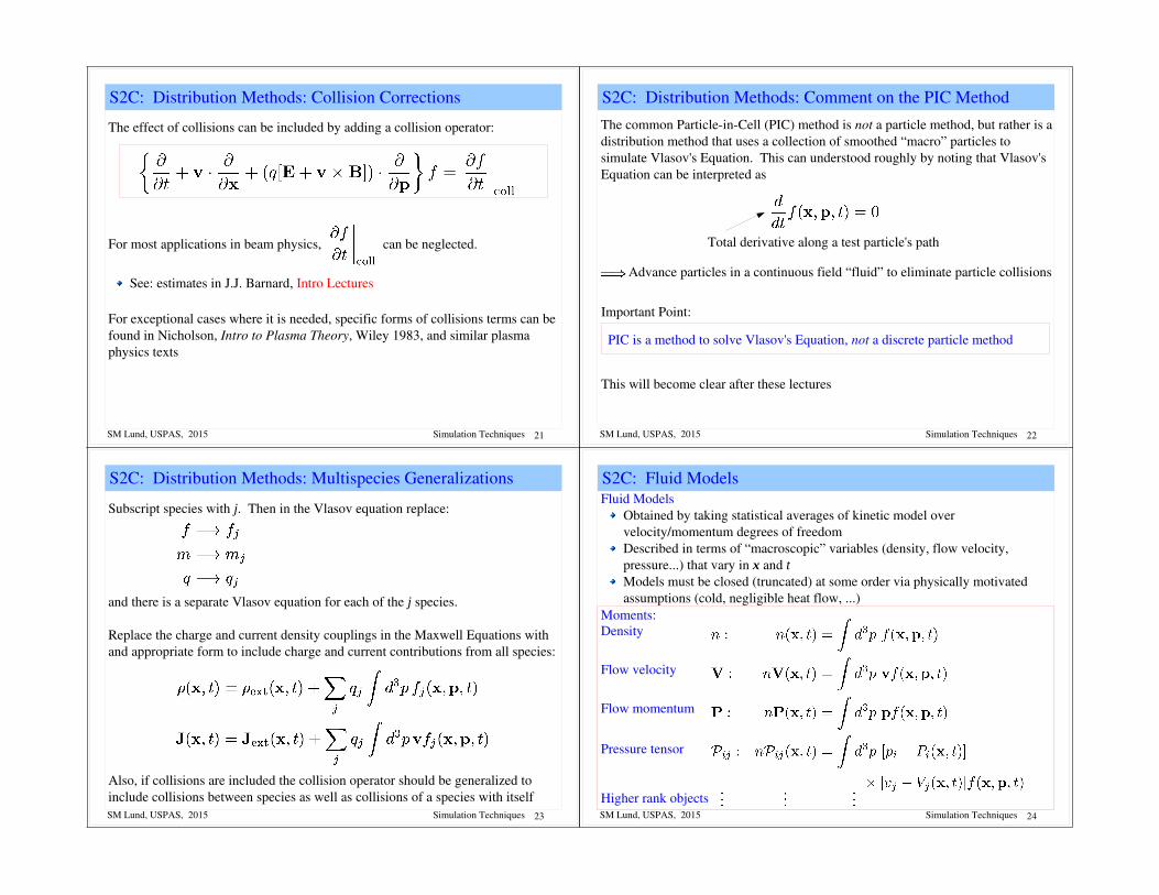
S2C: Distribution Methods: Collision Corrections
The effect of collisions can be included by adding a collision operator:
For most applications in beam physics, can be neglected.
For exceptional cases where it is needed, specific forms of collisions terms can be found in Nicholson, Intro to Plasma Theory, Wiley 1983, and similar plasma physics texts
See: estimates in J.J. Barnard, Intro Lectures
SM Lund, USPAS, 2015 22Simulation Techniques
S2C: Distribution Methods: Comment on the PIC Method
The common ParticleinCell (PIC) method is not a particle method, but rather is a distribution method that uses a collection of smoothed “macro” particles to simulate Vlasov's Equation. This can understood roughly by noting that Vlasov's Equation can be interpreted as
Important Point:
Total derivative along a test particle's path
PIC is a method to solve Vlasov's Equation, not a discrete particle method
This will become clear after these lectures
Advance particles in a continuous field “fluid” to eliminate particle collisions
SM Lund, USPAS, 2015 23Simulation Techniques
S2C: Distribution Methods: Multispecies Generalizations
Subscript species with j. Then in the Vlasov equation replace:
and there is a separate Vlasov equation for each of the j species.
Replace the charge and current density couplings in the Maxwell Equations with and appropriate form to include charge and current contributions from all species:
Also, if collisions are included the collision operator should be generalized to include collisions between species as well as collisions of a species with itself
SM Lund, USPAS, 2015 24Simulation Techniques
S2C: Fluid Models Fluid Models
Obtained by taking statistical averages of kinetic model over velocity/momentum degrees of freedomDescribed in terms of “macroscopic” variables (density, flow velocity, pressure...) that vary in x and tModels must be closed (truncated) at some order via physically motivated assumptions (cold, negligible heat flow, ...)
Density
Flow velocity
Pressure tensor
Higher rank objects
Flow momentum
Moments:

SM Lund, USPAS, 2015 25Simulation Techniques
S2C: Fluid Models: Equations of Motion Equations of Motion (Eulerian perspective)Continuity:
Force: ith component
Fields:Maxwell Equations are the same with charge and current density coupling to fluid variables given by:
Pressure: tensor component
SM Lund, USPAS, 2015 26Simulation Techniques
S2C: Fluid Model: Multispecies Generalization
Subscript species with j. Then in the continuity, force, pressure, ... equations replace
Replace the charge and current density couplings in the Maxwell Equations with
Particle Properties Moments
SM Lund, USPAS, 2015 27Simulation Techniques
S2C: Lagrangian Formulation of Distribution Methods
In kinetic and especially fluid models it can be convenient to adopt Lagrangian methods. For fluid models these can be distinguished as follows:
Eulerian Fluid Model:Flow quantities are functions of space (x) and and evolve in time (t)
Example: density n(x, t) and flow velocity V(x, t)
Lagrangian Fluid Model:Identify parts of evolution (flow) with objects (material elements) and follow the flow in time (t)
Shape and position of elements must generally evolve to represent flowExample: envelope model edge radii
Many distribution methods for Vlasov's Equation are hybrid Lagrangian methodsMacro particle “shapes” in PIC (Particle in Cell) method to be covered can be thought of as Lagrangian elements representing a Vlasov flow
SM Lund, USPAS, 2015 28Simulation Techniques
S2C: Example Lagrangian Fluid Model 1D Lagrangian model of the longitudinal evolution of a cold beam
Discretize fluid into longitudinal elements with boundariesDerive equations of motion for elements
slice boundaries
velocities of slice boundaries
fixed
fixedfor single species(set initial coordinates)
Lagrange.png
Coordinates:
Charges:
Masses:
Velocities:

SM Lund, USPAS, 2015 29Simulation Techniques
Example Lagrangian Fluid Model, Continued (2) Solve the (assume nonrelativisitic) equations of motion
for all the slice boundaries. Several methods might be used to calculate Ez:
1) Take “slices” to have some radial extent modeled by a perpendicular envelope etc. and deposit the Q
i+1/2 onto a grid and solve:
2) Employ a “gfactor” model
3) Pure 1D model using Gauss' Law
subject to
and extent of the elements etc.
SM Lund, USPAS, 2015 30Simulation Techniques
S2D: Moment Methods
Moment MethodsMost reduced description of an intense beam– Often employed in lattice designsBeam represented by a finite (closed and truncated) set of moments that are advanced from initial values– Here by moments, we mean functions of a single variable s or tSuch models are not generally selfconsistent– Some special cases such as a stable transverse KV equilibrium distribution
(see: S.M. Lund lectures on Transverse Equilibrium Distributions) are consistent with truncated moment description (rms envelope equation)
– Typically derived from assumed distributions with selfsimilar evolutionSee: S.M. Lund lectures on Transverse Equilibrium Distributions for more details on moment methods applied to transverse beam physics
SM Lund, USPAS, 2015 31Simulation Techniques
S2D: Moment Methods: 1st Order Moments Many moment models exist. Illustrate with examples for transverse beam evolutionMoment definition:
1st order moments:
Centroid coordinate
Centroid angle
Off momentum
Averages over the transverse degrees of freedom in the distribution
SM Lund, USPAS, 2015 32Simulation Techniques
S2D: Moment Methods: 2nd and Higher Order Moments
2nd order moments:
x moments dispersive momentsy moments xy cross moments
It is typically convenient to subtract centroid from higherorder moments
3rd order moments: Analogous to 2nd order case, but more for each order
SM Lund, USPAS, 2015 33Simulation Techniques
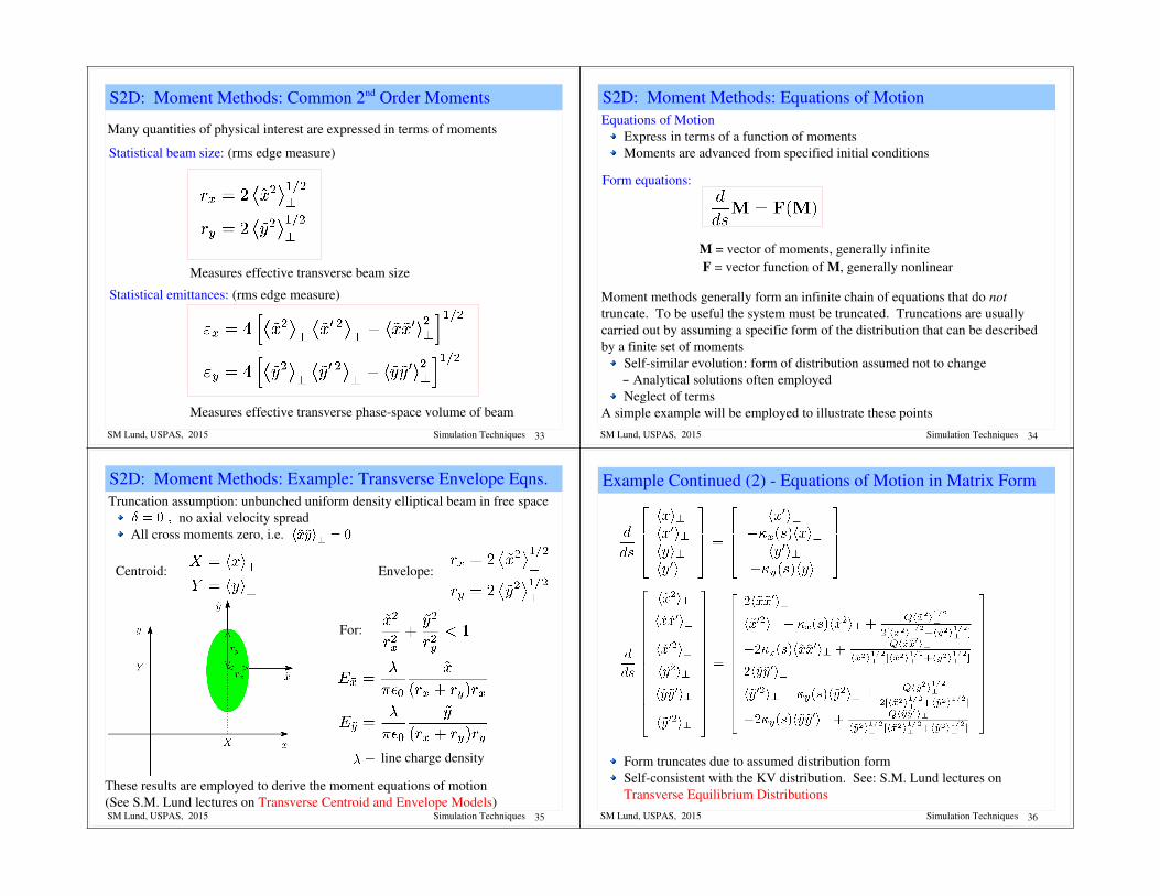
S2D: Moment Methods: Common 2nd Order Moments
Many quantities of physical interest are expressed in terms of moments
Statistical beam size: (rms edge measure)
Statistical emittances: (rms edge measure)
Measures effective transverse beam size
Measures effective transverse phasespace volume of beam
SM Lund, USPAS, 2015 34Simulation Techniques
S2D: Moment Methods: Equations of Motion Equations of Motion
Express in terms of a function of momentsMoments are advanced from specified initial conditions
Form equations:
M = vector of moments, generally infinite F = vector function of M, generally nonlinear
Moment methods generally form an infinite chain of equations that do not truncate. To be useful the system must be truncated. Truncations are usually carried out by assuming a specific form of the distribution that can be described by a finite set of moments
Selfsimilar evolution: form of distribution assumed not to change– Analytical solutions often employedNeglect of terms
A simple example will be employed to illustrate these points
SM Lund, USPAS, 2015 35Simulation Techniques
S2D: Moment Methods: Example: Transverse Envelope Eqns.
For:
These results are employed to derive the moment equations of motion (See S.M. Lund lectures on Transverse Centroid and Envelope Models)
Truncation assumption: unbunched uniform density elliptical beam in free space no axial velocity spreadAll cross moments zero, i.e.
line charge density
Centroid: Envelope:
SM Lund, USPAS, 2015 36Simulation Techniques
Example Continued (2) Equations of Motion in Matrix Form
Form truncates due to assumed distribution formSelfconsistent with the KV distribution. See: S.M. Lund lectures on Transverse Equilibrium Distributions

SM Lund, USPAS, 2015 37Simulation Techniques
Example Continued (3) Reduced Form Equations of Motion
The 2nd order moment equations can be equivalently expressed as
Using 2nd order moment equations we can show that
SM Lund, USPAS, 2015 38Simulation Techniques
Example Continued (4) : Contrast Form of Matrix and Reduced Form Moment Equations
Relative advantages of the use of coupled matrix form versus reduced equations can depend on the problem/situation
Coupled Matrix Equations Reduced Equations
etc.
M = Moment VectorF = Force Vector
Easy to formulate– Straightforward to incorporate
additional effectsNatural fit to numerical routine– Easy to code
Reduction based on identifying invariants such as
helps understand solutionsCompact expressions
SM Lund, USPAS, 2015 39Simulation Techniques
S2E: Hybrid Methods Beyond the three levels of modeling outlined earlier:
0) Particle methods1) Distribution methods2) Moment methods
there exist numerous “hybrid” methods that combine features of several methods.Hybrid methods may be the most common in detailed simulations.
Examples of Common Hybrid Methods:ParticleinCell (PIC) models Shaped (Lagrangian) macroparticles represent the distribution Macroparticles evolved using particle equations of motion Interactions via selffield are smoothed to represent continuum mechanics Gyrokinetic models– Average over fast gyro motion in strong magnetic fields: common in plasma
physicsDeltaf models– Evolve perturbed distribution with marker particles evolving about a core
“equilibrium” distribution
SM Lund, USPAS, 2015 40Simulation Techniques
Hybrid Methods Continued (2)
Comments on selecting methods:Particle and distribution methods are appropriate for higher levels of detailMoment methods are used for rapid iteration of machine design– Moments also typically calculated as diagnostics in particle and distribution
methodsEven within one (e.g. particle method) there are many levels of description:– Electromagnetic and electrostatic, with many field solution methods– 1D, 2D, 3D
Employing a hierarchy of models with full diagnostics allows crosschecking (both in numerics and physics) and aids understanding– No single method is best in all cases

SM Lund, USPAS, 2015 41Simulation Techniques
S3: Overview of Basic Numerical Methods S3A: Discretizations
General approach is to discretize independent variables in each of the methods and solve for dependent variables which in some cases may be discretized as wellTime (or s)
initial condition
time_discretization.png
Nonuniform meshes also possible– Add resolution where needed– Increases complexity
In applications may apply these descriptions in a variety of waysMove a transverse thin slice of a beam...
SM Lund, USPAS, 2015 42Simulation Techniques
Transverse Coordinate Discretization Spatial Coordinates (transverse)
Analogous for 3D, momentum coordinates (in direct Vlasov simulations), etc.Nonuniform meshes possible to add resolution where needed
space_discretization.png
SM Lund, USPAS, 2015 43Simulation Techniques
Transverse Coordinate Discretization – Applications
Thin slice of a long pulse is advanced and the transverse grid moves with the slice
In applications may apply these discretizations in a variety of ways:Transverse Slice Simulation:
Move a transverse thin “slice” of beam along the axial coordinate s of a reference particle
transverse_beam_slice.png
Limitations:– This “unbunched” approximation is not always possible– 3D effect can matter, e.g. in short pulses and/or beams ends
SM Lund, USPAS, 2015 44Simulation Techniques
Transverse Coordinate Discretization – Applications (2)
midpulse_diode.png
Steady State Simulation:Simulate the middle of a long pulse where a time stationary beam fills the grid
SourcePierce
Electrode Aperture
Mesh is stationary, leading to limitations– Beam pulse always has ends: see J.J. Barnard lectures on Longitudinal Physics– Assumes that the midpulse in nearly timeindependent in structure
Example: MidPulse Diode
SM Lund, USPAS, 2015 45Simulation Techniques
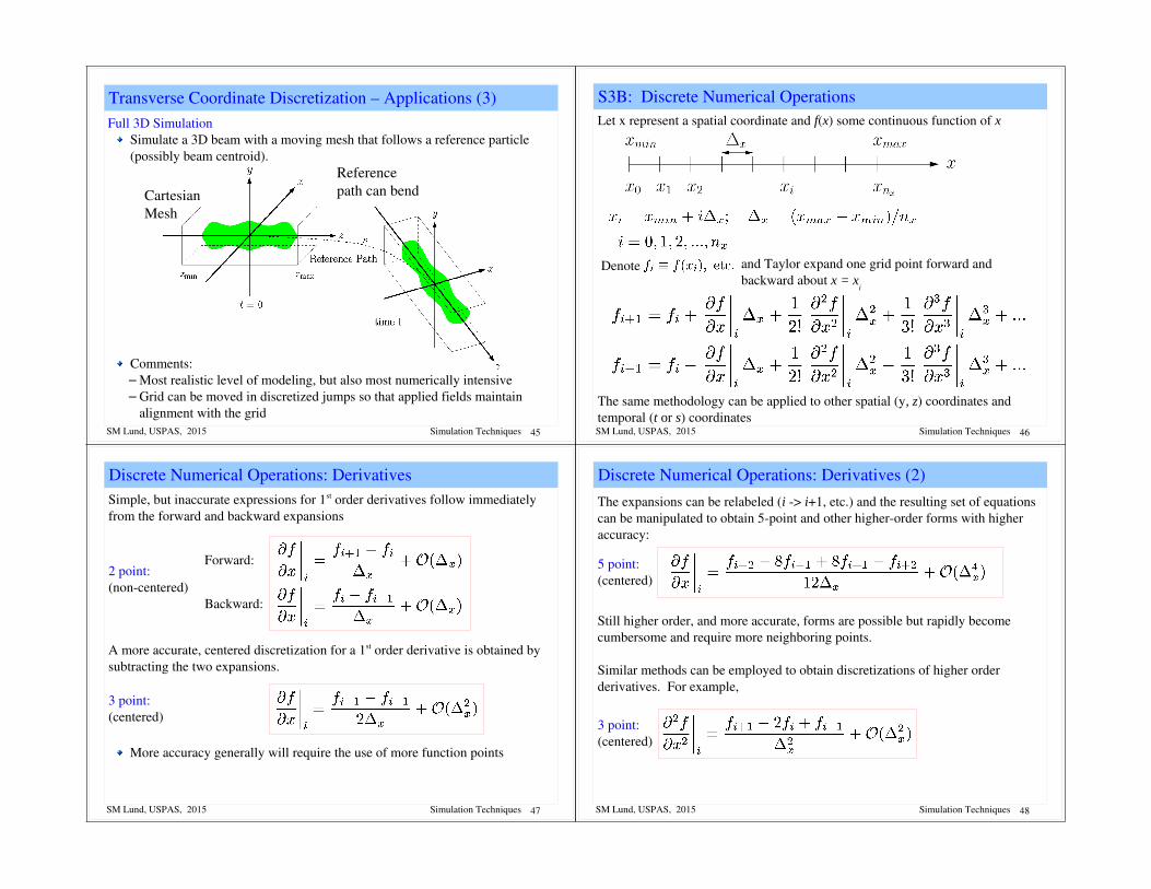
Transverse Coordinate Discretization – Applications (3)
3d_beam.png
Full 3D SimulationSimulate a 3D beam with a moving mesh that follows a reference particle (possibly beam centroid).
Comments:– Most realistic level of modeling, but also most numerically intensive– Grid can be moved in discretized jumps so that applied fields maintain
alignment with the grid
CartesianMesh
Referencepath can bend
SM Lund, USPAS, 2015 46Simulation Techniques
S3B: Discrete Numerical OperationsLet x represent a spatial coordinate and f(x) some continuous function of x
Denote and Taylor expand one grid point forward and backward about x = x
i
The same methodology can be applied to other spatial (y, z) coordinates and temporal (t or s) coordinates
x_discretization.png
SM Lund, USPAS, 2015 47Simulation Techniques
Discrete Numerical Operations: DerivativesSimple, but inaccurate expressions for 1st order derivatives follow immediately from the forward and backward expansions
Forward:
Backward:
A more accurate, centered discretization for a 1st order derivative is obtained by subtracting the two expansions.
3 point:(centered)
2 point:(noncentered)
More accuracy generally will require the use of more function points
SM Lund, USPAS, 2015 48Simulation Techniques
Discrete Numerical Operations: Derivatives (2)The expansions can be relabeled (i > i+1, etc.) and the resulting set of equations can be manipulated to obtain 5point and other higherorder forms with higher accuracy:
5 point:(centered)
Still higher order, and more accurate, forms are possible but rapidly become cumbersome and require more neighboring points.
Similar methods can be employed to obtain discretizations of higher order derivatives. For example,
3 point:(centered)
SM Lund, USPAS, 2015 49Simulation Techniques
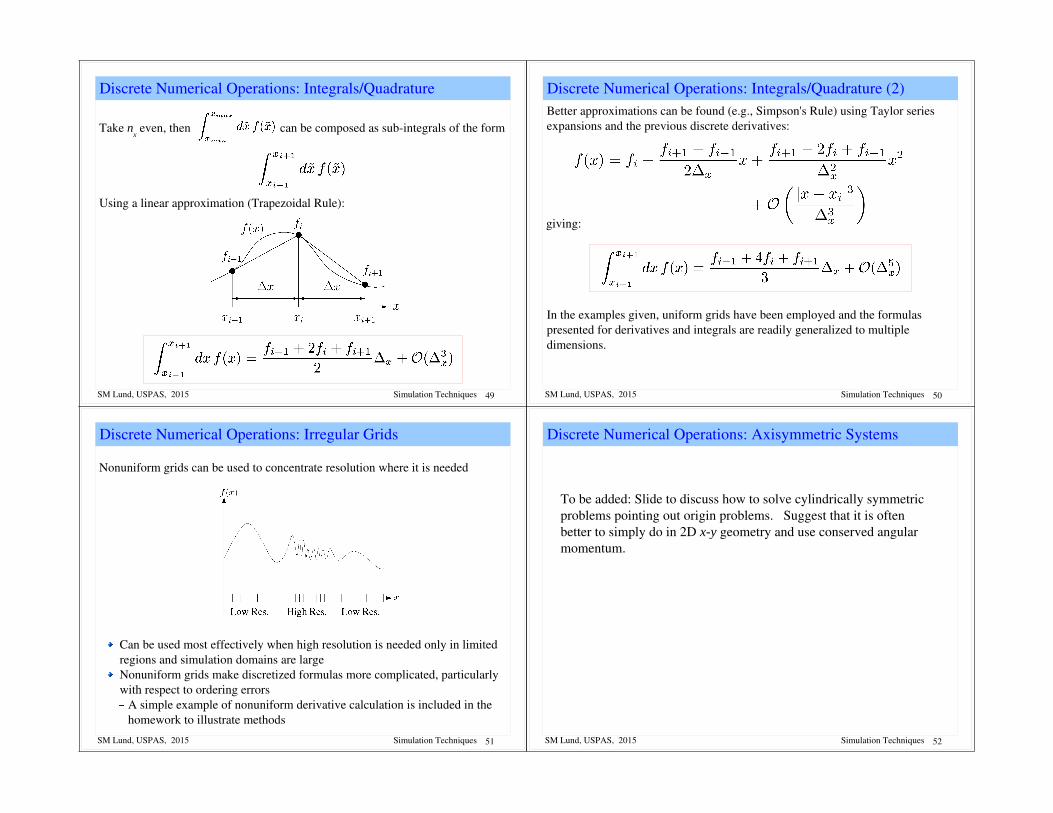
Discrete Numerical Operations: Integrals/Quadrature
Take nx even, then can be composed as subintegrals of the form
Using a linear approximation (Trapezoidal Rule): trapezoidal_rule.png
SM Lund, USPAS, 2015 50Simulation Techniques
Discrete Numerical Operations: Integrals/Quadrature (2)Better approximations can be found (e.g., Simpson's Rule) using Taylor series expansions and the previous discrete derivatives:
giving:
In the examples given, uniform grids have been employed and the formulas presented for derivatives and integrals are readily generalized to multiple dimensions.
SM Lund, USPAS, 2015 51Simulation Techniques
Discrete Numerical Operations: Irregular Grids
Nonuniform grids can be used to concentrate resolution where it is needed
Can be used most effectively when high resolution is needed only in limited regions and simulation domains are largeNonuniform grids make discretized formulas more complicated, particularly with respect to ordering errors– A simple example of nonuniform derivative calculation is included in the
homework to illustrate methods
irregular_grid.png
SM Lund, USPAS, 2015 52Simulation Techniques
Discrete Numerical Operations: Axisymmetric Systems
To be added: Slide to discuss how to solve cylindrically symmetric problems pointing out origin problems. Suggest that it is often better to simply do in 2D x-y geometry and use conserved angular momentum.

SM Lund, USPAS, 2015 53Simulation Techniques
S3C: Numerical Solution of Moment Methods – Time Advance
/// Example: Axisymmetric envelope equation for a continuously focused beam
We now have the tools to numerically solve moment methods. The moment equations may always be written as an Ndimensional set of coupled 1st order ODEs (see: S2C and S.M. Lund lectures on Transverse Envelope Equations):
Methods developed to advance moments can also be used for advances in particle and distribution methods
///
Ndim vector of moments
vector equation of motion
SM Lund, USPAS, 2015 54Simulation Techniques
S3C: Numerical Solution of Moment Methods – Euler Advance
Euler's Method: Apply the forward difference formula
Rearrange to obtain 1st order Euler advance:
Note that steps will lead to a total error
Error decreases only linearly with step sizeNumerical work for each step is only one evaluation of F
Moments advanced in discrete steps in s from initial values
SM Lund, USPAS, 2015 55Simulation Techniques
S3C: Numerical Solution of Moment Methods – Order Advance
Definition: A discrete advance with error is called an (n1)th order method
Euler's method is a 1st order methodHigher order methods are generally used for ODE's in moment methods– Numerical work to evaluate F smallLow order methods are generally used for particle and distribution methods– Numerical work to evaluate F large
SM Lund, USPAS, 2015 56Simulation Techniques
S3C: Numerical Solution of Moment Methods – RungeKutta Advance
RungeKutta Method:
Integrate from to :
Approximate F with a Taylor expansion through the midpoint of the step,
The linear term integrates to zero, leaving

SM Lund, USPAS, 2015 57Simulation Techniques
Higher order RungeKutta schemes are derived analogously from various quadrature formulas. Such formulas are found in standard numerical methods texts
Typically, methods with error will require N evaluations of F
Requires two evaluations of F per advance2nd order accurate in
RungeKutta Advance (2)
2nd Order RungeKutta Method:
Note: only need for apply Euler's method for the twostep procedure:
to Accuracy, so we can
Step 1:
Step 2:
SM Lund, USPAS, 2015 58Simulation Techniques
S3C: Numerical Solutions of Moment Methods
Many methods are employed to advance moments and particle orbits.
A general survey of these methods is beyond the scope of this lecture. But some general comments can be made:
Many higherorder methods with adaptive step sizes exist that refine accuracy to specified tolerances and are optimized for specific classes of equations Packages such as Mathematica and SciPy have many examplesChoice of numerical method often relates to numerical work and stability considerationsCertain methods can be formulated to exactly preserve relevant singleparticle invariants– “Symplectic” methods preserve Hamiltonian structure of dynamicsAccelerator problems can be demanding due to multiple frequency scales and long tracking times/distances– Hamiltonian dynamics; phase space volume does not decay
SM Lund, USPAS, 2015 59Simulation Techniques
S3C: Numerical Solutions of Moment Methods – Numerical Stability
“Numerical Reversibility” test of stability:In this method, the final value of an advance is used as an initial condition. Then the problem is run backwards to the original starting point and deviations from the initial conditions taken in the original advance are analyzed.
Provides a simple, but stringent test of accuracyWill ultimately fail due to roundoff errors and cases where there is a sensitive dependence on initial conditions Chaotic orbits a common exampleOrbits can be wrong but qualitatively right Lack of convergence does not necessarily mean results will be useless Right “pattern” in chaotic structures can be obtained with inaccurate orbits Will quantify better later
We will now briefly overview an application of moment equations, namely the KV envelope equations, to a practical high current transport lattice that was designed for Heavy Ion Fusion applications at Lawrence Berkeley National Laboratory.
SM Lund, USPAS, 2015 60Simulation Techniques
S3C: Moment Equation Application: Perp. KV Envelope Eqns Neglect image charges and nonlinear selffields (emittance constant) to obtain moment equations for the evolution of the beam envelope radii
Dimensionless Perveancemeasures spacecharge strength
RMS Edge Emittancemeasures xx' phasespace area~(beam size)sqrt(thermal temp.)
The matched beam solution together with parametric constraints from engineering, higherorder theory, and simulations are used to design the lattice.

SM Lund, USPAS, 2015 61Simulation Techniques
Application Example Continued (2) – Focusing Lattice
Magnetic Quadrupole
Electric Quadrupole
Rigidity
Focusing Strength
Take an alternating gradient FODO doublet lattice
SM Lund, USPAS, 2015 62Simulation Techniques
Application Example Contd. (3) – Matched Envelope Properties
IonK+, E = 2 MeVCurrentI = 800 mALattice
Envelope Properties:1) Low Emittance Case:
2) High Emittance Case:
env_match.png
SM Lund, USPAS, 2015 63Simulation Techniques
S4: Numerical Solution of Particle and Distribution MethodsS4A: OverviewParticle Methods – Generally not used at high spacecharge intensityDistribution Methods – Preferred (especially PIC) for high spacecharge. We will motivate why now.Why are direct particle methods are not a good choice for typical beams?
N particle coordinates
Physical beam (typical)N ~ 1010 – 1014 particles
Although larger problems are possible every year with more powerful computers, current processor speeds and memory limit us to N 108 particles
phasespace.png
SM Lund, USPAS, 2015 64Simulation Techniques
Numerical Solution of Particle and Distribution Methods (2)Represent the beam by Lagrangian “macroparticles” advanced in time
Same q/m ratio as real particle– Gives same single particle dynamics in the applied fieldMore collisions due to macroparticles having more close approaches– Enhanced collisionality is unphysical– Controlled by smoothing the macroparticle interaction with the selffield.
macroparticles.png
Macroparticle Properties:
Partition local density into macroparticles

SM Lund, USPAS, 2015 65Simulation Techniques
Numerical Solution of Particle and Distribution Methods (3)
Continuum distribution advanced on a discrete phasespace mesh– Extreme memory for high resolution. Example: for 4D x-p
x, y-p
y with 100
mesh points on each axis > 1004 = 108 values to store in fast memory (RAM)Discretization errors can lead to aliasing and unphysical behavior
(negative probability, etc.)
Direct Vlasov as an example:
Discretize grid points {xi, p
i}
Advance distribution f(x,p,t) at discrete grid points in time
phasespace_grid.png
SM Lund, USPAS, 2015 66Simulation Techniques
Numerical Solution of Particle and Distribution Methods (4)
Both particle and distribution methods can be broken up into two basic parts:0) Moving particles or distribution evaluated at grid points through a finite time
(or axial space) step1) Calculation of beam selffields consistently with the distribution of particles
In both methods, significant fractions of run time may be devoted to diagnosticsMoment calculations can be computationally intensive and may be “gathered” frequently for evolution “histories”Phase space projections (“snapshot” in time)Fields (snapshot in time)
Diagnostics are also critical!Without appropriate diagnostics runs are useless, even if correctMust accumulate and analyze/present large amounts of data in an understandable format
Significant code development time may also be devoted to creating (loading) the initial distribution of particles to simulate
Loading will usually only take a small fraction of total run time
SM Lund, USPAS, 2015 67Simulation Techniques
S4B: Integration of Equations of Motion
Higher order methods require more storage and numerical work per time stepFieldsolves are expensive, especially in 3D, and several fieldsolves per step can be necessary for higher order accuracy
Therefore, loworder methods are typically used for selfconsistent spacecharge. The “leapfrog” method is most common
Only need to store prior position and velocityOne fieldsolve per time step
Illustrate the leapfrog method for nonrelativistic particle equations of motion:
Develop methods for particles but can be applied to moments, distributions,...
SM Lund, USPAS, 2015 68Simulation Techniques
Leapfrog Method for Electric ForcesLeapfrog Method: for velocity independent (Electric) forcesLeapfrog Advance (time centered): Advance velocity and position out of phase
Velocity:
Position:
leapfrog.png
–

SM Lund, USPAS, 2015 69Simulation Techniques
Leapfrog Method: OrderTo analyze the properties of the leapfrog method it is convenient to write the map in an alternative form:
Subtract the two equations above and apply the other leapfrog advance formula:
Note correspondence of formula to discretized derivative:
Leapfrog method is 2nd order accurate
SM Lund, USPAS, 2015 70Simulation Techniques
Initial conditions must be desynchronized in leapfrog method
Leapfrog Method: SynchronizationSince x and v are not evaluated at the same time in the leapfrog method synchronization is necessary both to start the advance cycle and for diagnostics
Initial conditions: typically, v is pushed back half a cycle
When evaluating diagnostic quantities such as moments the particle coordinates and velocities should first be synchronized analogously to above
leapfrog_synch.png
SM Lund, USPAS, 2015 71Simulation Techniques
Leapfrog Method for Magnetic and Electric Forces The Boris MethodVelocity Dependent ForcesAnother complication in the evolution ensues when the force has velocity dependence, as occurs with magnetic forces. This complication results because x and v are advanced out of phase in the leapfrog method
velocity termElectric field E acceleratesMagnetic field B bends particle trajectory without change in speed |v|
A commonly implemented time centered scheme for magnetic forces is the following 3step “Boris” method:
J. Boris, in Proceedings of the 4th Conference on the Numerical Simulation of Plasmas (Naval Research Lab, Washington DC 1970)
SM Lund, USPAS, 2015 72Simulation Techniques
The Boris Advance
Boris Advance: The coordinate advance is the same as previous leapfrog and the velocity advance is modified as a 3 step procedure:1) Halfstep acceleration in electric field
2) Full step rotation in magnetic field. Here choose coordinates so that is along the zaxis and and resolve into components parallel/perpendicual to z
3) Halfstep acceleration in electric field

SM Lund, USPAS, 2015 73Simulation Techniques
Boris Advance Continued (2)
Complication: on startup, how does one generate the outofphase x, v advance from the initial conditions?
Calculate E, B with initial conditionsMove v backward half a time step– Rotate with B a halfstep– Decelerate a halfstep in E
Similar comments hold for synchronization of x, v for diagnostic accumulation
Now we will look at the numerical properties of the leapfrog advance cycleOnly use a simple “electric” force example to illustrate issues
SM Lund, USPAS, 2015 74Simulation Techniques
Leapfrog Advance: Errors and Numerical Stability
To better understand the leapfrog method consider the simple harmonic oscillator:
Discretized equation of motion
This has solutions for
Try a solution of the form
and it is straightforward to show via expansion that for small
Exact solution
SM Lund, USPAS, 2015 75Simulation Techniques
It follows for the leapfrog method applied to a simple harmonic oscillator:For the method is stableThere is no amplitude error in the integrationFor the phase error is
Actual phase:
Simulated phase:
Error phase:
Note: i to get to a fixed time and therefore phase errors decrease as
Leapfrog Errors and Numerical Stability Continued (2)
// Example:
Steps for a phase errorTime step
//
SM Lund, USPAS, 2015 76Simulation Techniques
Leapfrog Errors and Numerical Stability Continued (3)
Exact orbit(solid ellipse)
Numerical orbit(dashed ellipse)
Contrast: Numerical and Actual Orbit: Simple Harmonic Oscillator
Exact:
Numerical:
Emittance = (Phase Space Area)/
orbit_contrast.png

SM Lund, USPAS, 2015 77Simulation Techniques
The numerical orbit conserves phase space area regardless of the number of steps taken! The slight differences between the numerical and actual orbits can be removed by rescaling the angular frequency to account for the discrete step
More general analysis of the leapfrog method shows it has “symplectic” structure, meaning it preserves the Hamiltonian nature of the dynamicsSymplectic methods are important for long tracking problems (typical in accelerators) to obtain the right orbit structure – RungeKutta methods are not symplectic and can result in artificial
numerical damping in long tracking problems
Leapfrog Errors and Numerical Stability Continued (4)
SM Lund, USPAS, 2015 78Simulation Techniques
Example: Contrast of NonSymplectic and Symplectic Advances Contrast: Numerical and Actual Orbit for a Simple Harmonic Oscillator use scaled coordinates (max extents unity for analytical solution)Symplectic Leapfrog Advance:
lf_np100_ns5_xvxplot.png
Sinetype initial conditions
Cosinetype initial conditions
lf_np100_ns5_yvyplot.png
lf_np100_ns10_xvxplot.png
lf_np100_ns10_yvyplot.png
5 steps per period, 100 periods 10 steps per period, 100 periods
Numerical Orbit
Actual Orbit
SM Lund, USPAS, 2015 79Simulation Techniques
Example: Contrast of NonSymplectic and Symplectic Advances (2)
Contrast: Numerical and Actual Orbit for a Simple Harmonic OscillatorNonSymplectic 2nd Order RungeKutta Advance: (see earlier notes on RK advance)
rk2_np10_ns6_xvxplot.png
Sinetype initial conditions
Cosinetype initial conditions
rk2_np50_ns20_xvxplot.png
6 steps per period, 10 periods 20 steps per period, 50 periods
Numerical Orbit
Actual Orbit
rk2_np10_ns6_yvyplot.png rk2_np50_ns20_yvyplot.pngSM Lund, USPAS, 2015 80Simulation Techniques
Contrast: Numerical and Actual Orbit for a Simple Harmonic OscillatorNonSymplectic 4th Order RungeKutta Advance: (analog to notes on 2nd order RK adv)
rk4_np20_ns5_xvxplot.png
Sinetype initial conditions
Cosinetype initial conditions
rk4_np200_ns10_xvxplot.png
5 steps per period, 20 periods 10 steps per period, 200 periods
Numerical Orbit
Actual Orbit
rk4_np20_ns5_yvyplot.png rk4_np200_ns10_yvyplot.png
Example: Contrast of NonSymplectic and Symplectic Advances (3)

SM Lund, USPAS, 2015 81Simulation Techniques
Example: Leapfrog Stability Applied to the Nonlinear Envelope Equation in a Continuous Focusing Lattice For linear equations of motion, numerical stability requires:
Here, k is the wave number of the phase advance of the quantity evolving under the linear force. The continuous focusing envelope equation is nonlinear:
Several wavenumbers k can be expressed in the envelope evolution:
.... Depressed Particle Betatron Motion
.... Undepressed Particle Betatron Motion
.... Quadrupole Envelope Mode
.... Breathing Envelope ModeSM Lund, USPAS, 2015 82Simulation Techniques
Example: Leapfrog Stability and the Continuous Foc. Envelope Equation (2)
Expect that for the fastest (largest k) component determines stability.
Numerical simulations for an initially matched envelope with:
The highest kmode, the breathing mode, appears to determine stability, i.e.is the stability criterion. Other values of produce results in
agreement with this conclusion.
SM Lund, USPAS, 2015 83Simulation Techniques
Numerical simulations an initially matched envelope with:Note that numerical errors seed small amplitude mismatch and that the plot scale to the left is ~ 1013 , corresponding to numerical errors.
Example: Leapfrog Stability and the Continuous Foc. Envelope Equation (3)
SM Lund, USPAS, 2015 84Simulation Techniques
Comments of 2D and 3D Axisymmetric Particle Moves
To be added:
Comments on moving ring particles: 3D axisymmetry => particles rings, 3D axisymmetry => particles are infinite cylindrical shells. Angular momentum will be conserved for such particles (can rotate) Easier to do in many cases using xy movers

SM Lund, USPAS, 2015 85Simulation Techniques
S4C: Field SolutionThe selfconsistent calculation of beamproduced selffields is vital to accurately simulate forces acting on particles in intense beams
Techniques outlined here are also applicable to distribution methodsLinear structure of the Maxwell equations allow fields to be resolved into externally applied and self (beam generated) components
applied fields generated by magnets and electrodes
self fields generated by beam charges and currents
Sometimes calculated at high resolution in external codes and imported or specified via analytic formulasSometimes calculated from code fieldsolve via applied charges and currents and boundary conditions
At high beam intensities can be a large fraction (on average) of applied fieldsImportant to calculate with realistic boundary conditions
SM Lund, USPAS, 2015 86Simulation Techniques
Electrostatic Field Solution
For simplicity, we restrict analysis to electrostatic problems to illustrate methods:
The Maxwell equations to be solved for E are
Ba specified via another code or theory
Ea due to biased electrodes and E
s due to beam spacecharge
implies that we can always take and so
SM Lund, USPAS, 2015 87Simulation Techniques
Electrostatic Field Solution: Typical Problem
As an example, it might be necessary to solve (2D) fields of a beam within an electric quadrupole assembly.
specified on domain boundary or consistently to model assembly in free space
beam_lattice_2d.png
Quadrupole electrodes held at ±V
Beam beam_lattice_2d.png
SM Lund, USPAS, 2015 88Simulation Techniques
Electrostatic Field Solution by Green's FunctionFormally, the solution to can be constructed with a Green's function, illustrated here with Dirichlet boundary conditions:
This yields (Jackson, Classical Electrodynamics)
Selffield component Applied field from electrode potentials
Definitions:
Unit normal vector to boundary surface
SM Lund, USPAS, 2015 89Simulation Techniques
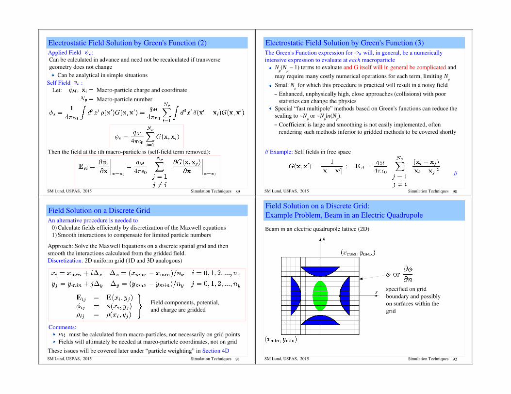
Electrostatic Field Solution by Green's Function (2)
Macroparticle charge and coordinate
Can be calculated in advance and need not be recalculated if transverse geometry does not change
Then the field at the ith macroparticle is (selffield term removed):
Can be analytical in simple situations
Macroparticle number
Let:Self Field :
Applied Field :
SM Lund, USPAS, 2015 90Simulation Techniques
Electrostatic Field Solution by Green's Function (3)The Green's Function expression for will, in general, be a numerically intensive expression to evaluate at each macroparticle
Np(N
p – 1) terms to evaluate and G itself will in general be complicated and
may require many costly numerical operations for each term, limiting Np
Small Np for which this procedure is practical will result in a noisy field
– Enhanced, unphysically high, close approaches (collisions) with poor statistics can change the physics
Special “fast multipole” methods based on Green's functions can reduce the scaling to ~N
p or ~N
pln(N
p).
– Coefficient is large and smoothing is not easily implemented, often rendering such methods inferior to gridded methods to be covered shortly
// Example: Self fields in free space
//
SM Lund, USPAS, 2015 91Simulation Techniques
Field Solution on a Discrete GridAn alternative procedure is needed to
0) Calculate fields efficiently by discretization of the Maxwell equations1) Smooth interactions to compensate for limited particle numbers
Approach: Solve the Maxwell Equations on a discrete spatial grid and then smooth the interactions calculated from the gridded field.Discretization: 2D uniform grid (1D and 3D analogous)
Field components, potential, and charge are gridded
Comments: must be calculated from macroparticles, not necessarily on grid pointsFields will ultimately be needed at marcoparticle coordinates, not on grid
These issues will be covered later under “particle weighting” in Section 4DSM Lund, USPAS, 2015 92Simulation Techniques
Field Solution on a Discrete Grid:Example Problem, Beam in an Electric Quadrupole
specified on grid boundary and possibly on surfaces within the grid
Beam in an electric quadrupole lattice (2D)
beam_lattice_2d_grid.png
SM Lund, USPAS, 2015 93Simulation Techniques
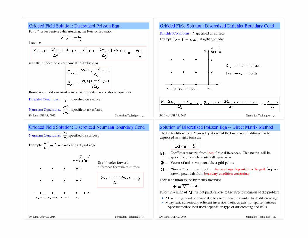
Gridded Field Solution: Discretized Poisson Eqn.For 2nd order centered differencing, the Poisson Equation
with the gridded field components calculated as
Boundary conditions must also be incorporated as constraint equations
Dirichlet Conditions:
Neumann Conditions:
specified on surfaces
specified on surfaces
becomes
SM Lund, USPAS, 2015 94Simulation Techniques
Gridded Field Solution: Discretized Dirichlet Boundary Cond
Dirichlet Conditions:
Example:
specified on surface
at right grid edge
For cells
Dirichlet.png
SM Lund, USPAS, 2015 95Simulation Techniques
Gridded Field Solution: Discretized Neumann Boundary Cond
Neumann Conditions:
Example:
specified on surfaces
at right grid edge
Neumann.png
Use 1st order forward difference formula at surface
SM Lund, USPAS, 2015 96Simulation Techniques
will in general be sparse due to use of local, loworder finite differencingMany fast, numerically efficient inversion methods exist for sparse matrices– Specific method best used depends on type of differencing and BC's
Solution of Discretized Poisson Eqn Direct Matrix MethodThe finitedifferenced Poisson Equation and the boundary conditions can be expressed in matrix form as:
Coefficients matrix from local finite differences. This matrix will be sparse, i.e., most elements will equal zeroVector of unknown potentials at grid points
“Source” terms resulting from beam charge deposited on the grid and known potentials from boundary condition constraints
Formal solution found by matrix inversion:
Direct inversion of is not practical due to the large dimension of the problem

SM Lund, USPAS, 2015 97Simulation Techniques
Example Discretized Field Solution
To illustrate this procedure, consider a simple 1D example with Dirichlet BC's
Discretize to :
Note: irrelevant
Correspond to surface terms that fix boundary condition potentials
rho_1d_Dirichlet.png
SM Lund, USPAS, 2015 98Simulation Techniques
Example Discretized Field Solution (2)
Matrix has tridiagonal structure and can be rapidly inverted using optimized numerical methods to efficiently calculate the
Sparse matrices need not be stored in full (waste of memory)
The 1D discretized Poisson equation and boundary conditions can be expressed in matrix form as:
SM Lund, USPAS, 2015 99Simulation Techniques
S4: Particle Methods – Field Solution Methods on Grid
Many other methods exist to solve the discretized field equations. These methods fall into three broad classes:1) Direct Matrix Methods
Fast inversion of sparse matrix2) Spectral Methods
Fast Fourier Transform (FFT)– Periodic boundary conditions– Sine transform ( on grid boundary)– FFT + capacity matrix for arbitrary conductors– Free space boundary conditions
3) Relaxation MethodsSuccessive overrelaxation (SOR)– General boundary conditions and structuresMultigrid (good, fast, and accurate method for complicated boundaries)
SM Lund, USPAS, 2015 100Simulation Techniques
Field Solution Methods on Grid Continued (2)
Sometimes methods in these three classes are combined. For example, one might employ spectral methods transversely and invert the tridiagonal matrix longitudinally.
Other discretization procedures are also widely employed, giving rise to other classes of field solutions such as:
Finite elementsVariationalMonte Carlo
Methods of field solution are central to the efficient numerical solution of intense beam problems. It is not possible to review them all here. But before discussing particle weighting, we will first overview the important spectral methods and FFT's

SM Lund, USPAS, 2015 101Simulation Techniques
Spectral Methods and the FFT
The spectral approach combined with numerically efficient Fast Fourier Transforms (FFT's) is commonly used to efficiently solve the Poisson Equation on a discrete spatial grid
Approach provides spectral information on fields that can be used to smooth the interactionsEfficiency of method enabled progress in early simulations in the 1960s– Computers had very limited memory and speedMethod remains important and can be augmented in various ways to implement needed boundary conditions– Simple to code using numerical libraries for FFT– Efficiency still important ... especially in 3D geometries
SM Lund, USPAS, 2015 102Simulation Techniques
Spectral Method: Discrete Fourier TransformIllustrate in 1D for simplicity (multidimensional case analogous)
Continuous Fourier Transforms (Reminder)
Transform Poisson Equation:
Similar procedures work to calculate the field on a finite, discrete spatial gridDevelop by analogy to continuous transforms
SM Lund, USPAS, 2015 103Simulation Techniques
// Aside: Transform conventions and notation vary
//
Physics convention:Reflects common usage in dynamics and quantum mechanics
Symmetrical convention:Factors of used symmetrically can be convenient numerically
Sometimes
Subtlety:If as then k must contain a large enough positive imaginary part for transform to exist and contour to carry out inversion contour must be taken consistently
SM Lund, USPAS, 2015 104Simulation Techniques
Discrete Fourier Transform (2)Discretize the problem as follows:
The discrete transform is the defined by analogy to the continuous transform by:
Analogy
In this section we employ j as a grid index to avoid confusion with

SM Lund, USPAS, 2015 105Simulation Techniques
Discrete Fourier Transform (3)
Note that is periodic in n with period nx
Then an inverse transform can be constructed exactly:
Let so n and j have the same ranges
This exact inversion is proved in the problems by summing a geometric series
SM Lund, USPAS, 2015 106Simulation Techniques
Spectral Methods: Aliasing
The discrete transform describes a periodic problem if indices are extendedDiscretization errors (aliasing) can occur
Figure to be edited:
Plots will be replaced with real transforms based on a Gaussian distribution in future versions of the notes
SM Lund, USPAS, 2015 107Simulation Techniques
Discrete Transform FormulasApplication of the Discrete Fourier Transform to solve Poisson's Equation:
Applying the discrete transform yields:
Poisson's Equation becomes:
Note: factors of Kn
2 need only be calculated once per simulation (store values)SM Lund, USPAS, 2015 108Simulation Techniques
Derivation of Discrete Transform Eqns./// Example Derivation of a formula for the discrete transformed Efield:
Substitute transforms into difference formula:
Discretized Efield
Transforms

SM Lund, USPAS, 2015 109Simulation Techniques
This equation must hold true for each term in the sum proportional to
to be valid for a general j.
///
SM Lund, USPAS, 2015 110Simulation Techniques
Spectral Methods: Discrete Transform Field Solution
Typical discrete Fourier transform field solution (not optimized)
ForwardTransform
MultiplyInverseTransform
FiniteDifference
DFT IDFT
Kn
2 factors can be calculated once and stored to increase numerical efficiency
SM Lund, USPAS, 2015 111Simulation Techniques
Discussion of Spectral Methods and the FFT
The Fast Fourier Transform (FFT) makes this procedure numerically efficientDiscrete transform (no optimization), ~(n
x + 1)2 complex operations
FFT exploits symmetries to reduce needed operations to ~ (nx + 1)ln(n
x + 1)
– Huge savings for large nx
The needed symmetries exist only for certain numbers of grid points. In the simplest manifestations: n
x + 1 = 2p, p = 1, 2, 3, ...
– Reduced freedom in grid choices– Other manifestations allow n
x + 1 = 2p and products of prime numbers for
more possibilitiesThe FFT can be combined with other procedures such as capacity matrices to implement boundary conditions for interior conductors, etc.
Allows rapid field solutions in complicated conductor geometries when capacity matrix elements can be precalculated and storedSymmetries can be exploited using 4x domain size to implement freespace boundary conditions (see Hockney and Eastwood)
FFT is the fastest method for simple geometrySimple to code using typical numerical libraries for FFT's
SM Lund, USPAS, 2015 112Simulation Techniques
S4D: Weighting: Depositing Particles on the Field Mesh and Interpolating Gridded Fields to Particles
We have outlined methods to solve the electrostatic Maxwell's equations on a discrete spatial grid. To complete the description we must:
Specify how to deposit macroparticle charges and current onto the gridSpecify how to interpolate fields on the spatial grid points to the macroparticle coordinates (not generally on the grid) to apply in the particle advanceSmooth interactions resulting from the small number of macroparticles to reduce artificial collisions resulting from the use of an unphysically small number of macroparticles needed for rapid simulation
This is called the particle weighting problem
SM Lund, USPAS, 2015 113Simulation Techniques
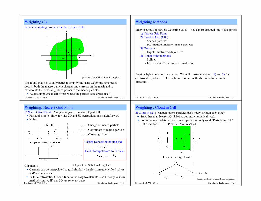
Weighting (2)Particle weighting problem for electrostatic fields
It is found that it is usually better to employ the same weighting schemes to deposit both the macroparticle charges and currents on the mesh and to extrapolate the fields at gridded points to the macroparticles
Avoids unphysical selfforces where the particle accelerates itself
bl_fig_22b.png
[Adapted from Birdsall and Langdon]
SM Lund, USPAS, 2015 114Simulation Techniques
Weighting Methods
Many methods of particle weighting exist. They can be grouped into 4 categories:1) Nearest Grid Point2) Cloud in Cell (CIC)
Shaped particles PIC method, linearly shaped particles
3) Multipole Dipole, subtracted dipole, etc.
4) Higher order methods Splines k-space cutoffs in discrete transforms
Possible hybrid methods also exist. We will illustrate methods 1) and 2) for electrostatic problems. Descriptions of other methods can be found in the literature.
SM Lund, USPAS, 2015 115Simulation Techniques
Weighting: Nearest Grid Point1) Nearest Grid Point: Assign charges to the nearest grid cell
Fast and simple: Show for 1D; 2D and 3D generalization straightforwardNoisy
Charge of macroparticle
Closest grid cell
Charge Deposition on ith Grid:
Field “Interpolation” to Particle:
Coordinate of macroparticle
bl_fig_26a.pngbl_fig_26a.pngComments:
Currents can be interpolated to grid similarly for electromagnetic field solves and/or diagnostics In 1D electrostatics Green's function is easy to calculate; use 1D only to show method simply; 2D and 3D are relevant cases
[Adapted from Birdsall and Langdon]
bl_fig_26a.png
SM Lund, USPAS, 2015 116Simulation Techniques
Weighting : Cloud in Cell2) Cloud in Cell: Shaped macroparticles pass freely through each other
Smoother than Nearest Grid Point, but more numerical workFor linear interpolation results in simple, commonly used “Particle in Cell” (PIC) method
bl_fig_26b.png
[Adapted from Birdsall and Langdon]
SM Lund, USPAS, 2015 117Simulation Techniques
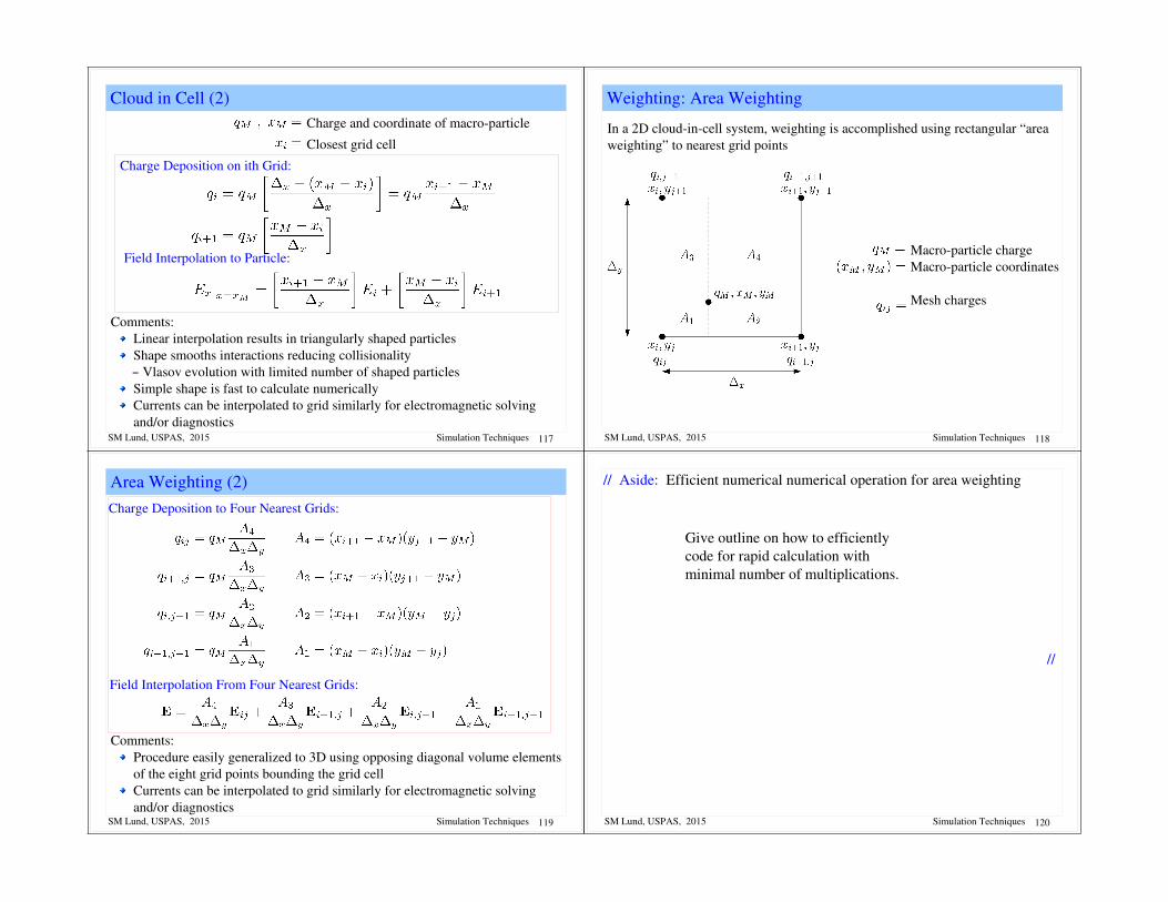
Cloud in Cell (2)Charge and coordinate of macroparticle
Closest grid cell
Charge Deposition on ith Grid:
Field Interpolation to Particle:
Comments:Linear interpolation results in triangularly shaped particlesShape smooths interactions reducing collisionality– Vlasov evolution with limited number of shaped particlesSimple shape is fast to calculate numericallyCurrents can be interpolated to grid similarly for electromagnetic solving and/or diagnostics
SM Lund, USPAS, 2015 118Simulation Techniques
Weighting: Area Weighting
In a 2D cloudincell system, weighting is accomplished using rectangular “area weighting” to nearest grid points
Macroparticle chargeMacroparticle coordinates
Mesh charges
area_weighting.png
SM Lund, USPAS, 2015 119Simulation Techniques
Area Weighting (2)
Comments:Procedure easily generalized to 3D using opposing diagonal volume elements of the eight grid points bounding the grid cell Currents can be interpolated to grid similarly for electromagnetic solving and/or diagnostics
Charge Deposition to Four Nearest Grids:
Field Interpolation From Four Nearest Grids:
SM Lund, USPAS, 2015 120Simulation Techniques
// Aside: Efficient numerical numerical operation for area weighting
//
Give outline on how to efficiently code for rapid calculation with minimal number of multiplications.
SM Lund, USPAS, 2015 121Simulation Techniques
Higher Order Weighting: Splines
To be added: Slide on Splines toillustrate what is meant by higher order methodsMake Points: Requires more numerical work and harder to code Some schemes can introduce neg probability problems Should evaluate against simpler low order methods using same computer power to see which method wins.
SM Lund, USPAS, 2015 122Simulation Techniques
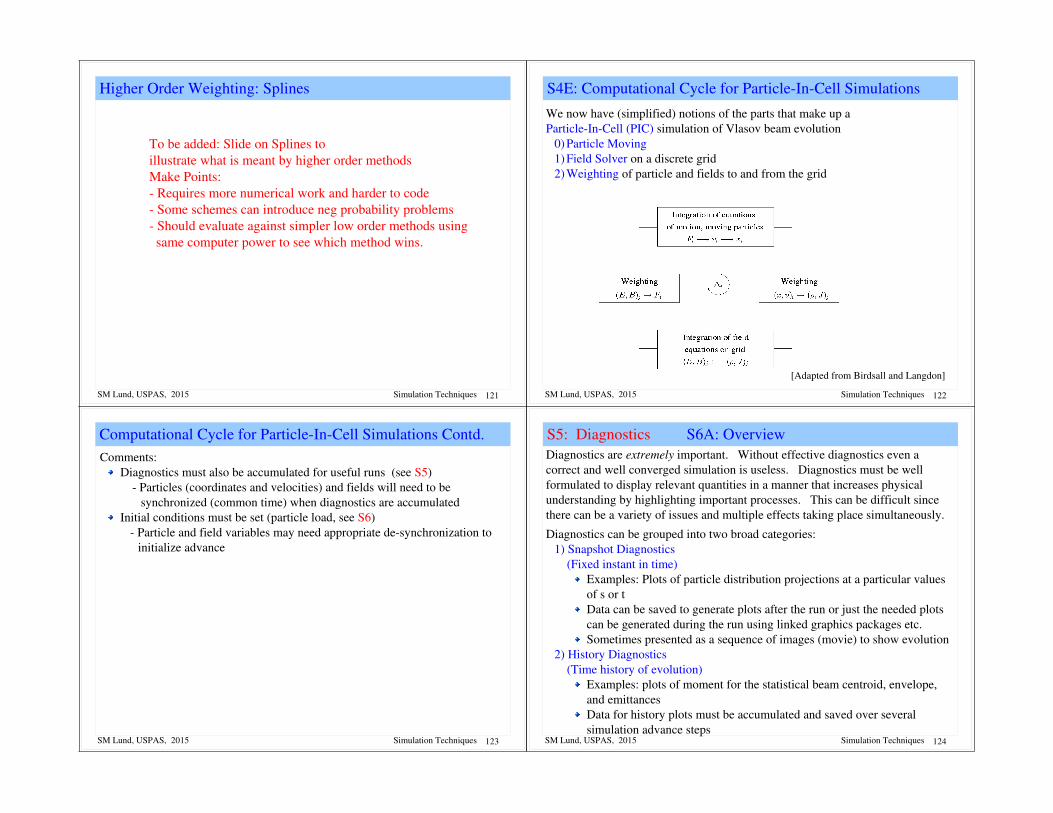
S4E: Computational Cycle for ParticleInCell Simulations
We now have (simplified) notions of the parts that make up a ParticleInCell (PIC) simulation of Vlasov beam evolution
0) Particle Moving1) Field Solver on a discrete grid2) Weighting of particle and fields to and from the grid
bl_fig_2.3a.png
[Adapted from Birdsall and Langdon]
SM Lund, USPAS, 2015 123Simulation Techniques
Computational Cycle for ParticleInCell Simulations Contd.Comments:
Diagnostics must also be accumulated for useful runs (see S5) Particles (coordinates and velocities) and fields will need to be
synchronized (common time) when diagnostics are accumulatedInitial conditions must be set (particle load, see S6)
Particle and field variables may need appropriate desynchronization to initialize advance
SM Lund, USPAS, 2015 124Simulation Techniques
S5: Diagnostics S6A: OverviewDiagnostics are extremely important. Without effective diagnostics even a correct and well converged simulation is useless. Diagnostics must be well formulated to display relevant quantities in a manner that increases physical understanding by highlighting important processes. This can be difficult since there can be a variety of issues and multiple effects taking place simultaneously.
Diagnostics can be grouped into two broad categories:1) Snapshot Diagnostics (Fixed instant in time)
Examples: Plots of particle distribution projections at a particular values of s or tData can be saved to generate plots after the run or just the needed plots can be generated during the run using linked graphics packages etc.Sometimes presented as a sequence of images (movie) to show evolution
2) History Diagnostics (Time history of evolution)
Examples: plots of moment for the statistical beam centroid, envelope, and emittancesData for history plots must be accumulated and saved over several simulation advance steps
SM Lund, USPAS, 2015 125Simulation Techniques
Snapshot Diagnostics: Particle PhaseSpace ProjectionsTo be added.
SM Lund, USPAS, 2015 126Simulation Techniques
Snapshot Diagnostics: FieldsTo be added.
SM Lund, USPAS, 2015 127Simulation Techniques
History Diagnostics: Moment EvolutionsMoments typically have a lesser degree of noise since they generally average over many macroparticles
2D case => full beam 3D case => local zslice of beam
Moments commonly of interest include:Centroid Measures how far beam is offcenter (from design orbit)
SM Lund, USPAS, 2015 128Simulation Techniques
rms Beam Extent Gives size of the beam Specifies “match” of periodic focusing flutter to lattice

SM Lund, USPAS, 2015 129Simulation Techniques
rms Phase Space Area (Emittance)
SM Lund, USPAS, 2015 130Simulation Techniques
S6: Initial Distributions and Particle LoadingS6A: OverviewTo start the large particle or distribution simulations, the initial distribution function of the beam must be specified.
For direct Vlasov simulations the distribution need simply be deposited on the phasespace grid
For PIC simulations, an appropriate distribution of macroparticle phasespace coordinates must be generated or “loaded” to represent the Vlasov distributionDiscussion:In realistic accelerators, focusing elements are svarying. In such situations there are no known smooth equilibrium distributions.
The KV distribution is an exact equilibrium for linear focusing fields, but has unphysical (singular) structure in 4dimensional transverse phasespace
Moreover, it is unclear in most cases if the beam is even best thought of as an equilibrium distribution as is typical in plasma physics. In accelerators, the beam in generally injected from a source and may only reside in the machine (especially for a linac) for a small number of characteristic oscillation periods and may not fully relax to an equilibrium like state within the machine.
SM Lund, USPAS, 2015 131Simulation Techniques
The lack of known, physically reasonable equilibria and the fact that the beams are injected from a source motivates socalled “sourcetotarget” simulations where particles are simulated off the source and tracked to the target. Such first principles simulations are most realistic if carried out with the actual focusing fields, accelerating waveforms, alignment errors, etc. Sourcetotarget simulations are highly valuable to measure expected machine performance. However, ideal sourcetotarget simulations can rarely be carried out due to:
Source is often incompletely described Example: important alignment and material errors may not be known
Source may contain physics not adequately in imperfectly modeled Example: plasma injectors with complicated material physics, etc.
Computer limitations: Memory required and simulation time Convergence and accuracies Limits of numerical methods applied Ex: singular description needed for ChildLangmuir model of spacecharge limited injection
Initial Distributions: SourcetoTarget Simulations
SM Lund, USPAS, 2015 132Simulation Techniques
Due to the practical difficulty of always carrying out simulations off the source, two alternative methods are commonly applied:
1) Load an idealized initial distributionSpecify at some specific time Based on physically reasonable theory assumptions
2) Load experimentally measured distributionConstruct/synthesize a distribution based on experimental measurements
Discussion:The 2nd option of generating a distribution from experimental measurements, unfortunately, often has practical difficulties:
Real diagnostics often are far from ideal 6D snapshots of beam phasespace Distribution must be reconstructed from partial data Typically many assumptions must be made in the synthesis process
Process of measuring the beam can itself change the beam It can sometimes be helpful to understand processes and limitations starting from cleaner, more idealized initial beam states
Initial Distributions: Types of Specified Loads

SM Lund, USPAS, 2015 133Simulation Techniques
Discussion Continued:Because of the practical difficulties of loading a distribution based exclusively on experimental measurements, idealized distributions are often loaded:
Employ distributions based on reasonable, physical ansatzesUse limited experimental measures to initialize:
Energy, current, rms equivalent beam sizes and emittances Simpler initial state can often aid insight:
Fewer simultaneous processes can allow one to more clearly understand how limits arise Seed perturbations of relevance when analyzing resonance effects, instabilities, halo, etc.
A significant complication is that there are no known exact smooth equilibrium distribution functions valid for periodic focusing channels:
Approximate theories valid for low phase advances may exist Startsev, Davidson, Struckmeier, and others
Formulate a simple approximate procedure to load an initial distribution that reflects features one would expect of an equilibrium
SM Lund, USPAS, 2015 134Simulation Techniques
S6B: KV Load and the rms Equivalent Beam
See handwritten notes from USPAS 06/08Will be updated in future versions of the notes
SM Lund, USPAS, 2015 135Simulation Techniques
S6C: Beam Envelope Matching
To be added in future versions.
SM Lund, USPAS, 2015 136Simulation Techniques
S6D: SemiGaussian Load
See handwritten notes from USPAS 06/08Will be updated in future versions of the notes

SM Lund, USPAS, 2015 137Simulation Techniques
Simple psudoequilibrium initial distribution:Use rms equivalent measures to specify the beam
Natural set of parameters for accelerator applicationsMap rms equivalent beam to a smooth, continuous focused matched beam
Use smooth core models that are stable in continuous focusing: Waterbag Equilibrium Parabolic Equilibrium
Thermal Equilibrium
Transform continuous focused beam for rms equivalency with original beam specification
Use KV transforms to preserve uniform beam CourantSnyder invariants
Procedure will apply to any svarying focusing channelFocusing channel need not be periodicBeam can be initially rms equivalent matched or mismatched if launched in a periodic transport channelCan apply to both 2D transverse and 3D beams
See Notes on: Transverse Equilibrium Distributions
S6E: Initial PseudoEquilbrium Distributions Based on Continuous Focusing Equilibria
SM Lund, USPAS, 2015 138Simulation Techniques
Procedure for Initial Distribution Specification
Step 1:For each particle (3D) or slice (2D) specify 2nd order rms properties at axial coordinate s
Assume focusing lattice is given:
specified
Envelope coordinates/angles:
Emittance:
Perveance:
Strength usually set by specifying undperessed phase advances
SM Lund, USPAS, 2015 139Simulation Techniques
Procedure for Initial Distribution Specification (2)
If the beam is rms matched, we take:
Not necessary even for periodic lattices Procedure applies to mismatched beams
SM Lund, USPAS, 2015 140Simulation Techniques
Procedure for Initial Distribution Specification (3)
Step 2:Define an rms matched, continuously focused beam in each transverse sslice:
Continuous sVarying
Envelope Radius
Emittance
Perveance
Define a (local) matched beam focusing strength in continuous focusing:0
SM Lund, USPAS, 2015 141Simulation Techniques
Procedure for Initial Distribution Specification (4)
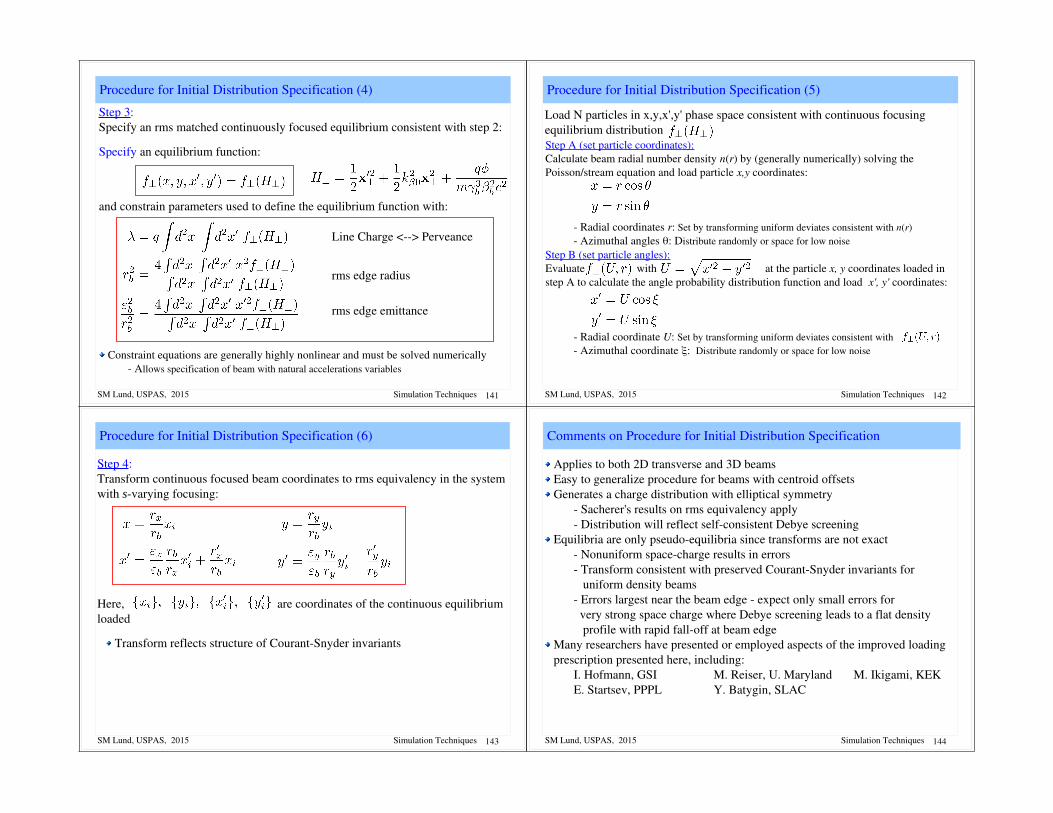
Step 3:Specify an rms matched continuously focused equilibrium consistent with step 2:
Specify an equilibrium function:
and constrain parameters used to define the equilibrium function with:
Line Charge <> Perveance
rms edge radius
rms edge emittance
Constraint equations are generally highly nonlinear and must be solved numerically Allows specification of beam with natural accelerations variables
SM Lund, USPAS, 2015 142Simulation Techniques
Procedure for Initial Distribution Specification (5)
Load N particles in x,y,x',y' phase space consistent with continuous focusing equilibrium distributionStep A (set particle coordinates):Calculate beam radial number density n(r) by (generally numerically) solving the Poisson/stream equation and load particle x,y coordinates:
Radial coordinates r: Set by transforming uniform deviates consistent with n(r) Azimuthal angles q: Distribute randomly or space for low noise
Step B (set particle angles):Evaluate with at the particle x, y coordinates loaded in step A to calculate the angle probability distribution function and load x', y' coordinates:
Radial coordinate U: Set by transforming uniform deviates consistent with Azimuthal coordinate x: Distribute randomly or space for low noise
SM Lund, USPAS, 2015 143Simulation Techniques
Procedure for Initial Distribution Specification (6)
Step 4:Transform continuous focused beam coordinates to rms equivalency in the system with svarying focusing:
Here, are coordinates of the continuous equilibrium loaded
Transform reflects structure of CourantSnyder invariants
SM Lund, USPAS, 2015 144Simulation Techniques
Applies to both 2D transverse and 3D beamsEasy to generalize procedure for beams with centroid offsetsGenerates a charge distribution with elliptical symmetry
Sacherer's results on rms equivalency apply Distribution will reflect selfconsistent Debye screening
Equilibria are only pseudoequilibria since transforms are not exact Nonuniform spacecharge results in errors Transform consistent with preserved CourantSnyder invariants for uniform density beams Errors largest near the beam edge expect only small errors for very strong space charge where Debye screening leads to a flat density profile with rapid falloff at beam edge
Many researchers have presented or employed aspects of the improved loading prescription presented here, including:
I. Hofmann, GSI M. Reiser, U. Maryland M. Ikigami, KEKE. Startsev, PPPL Y. Batygin, SLAC
Comments on Procedure for Initial Distribution Specification
SM Lund, USPAS, 2015 145Simulation Techniques
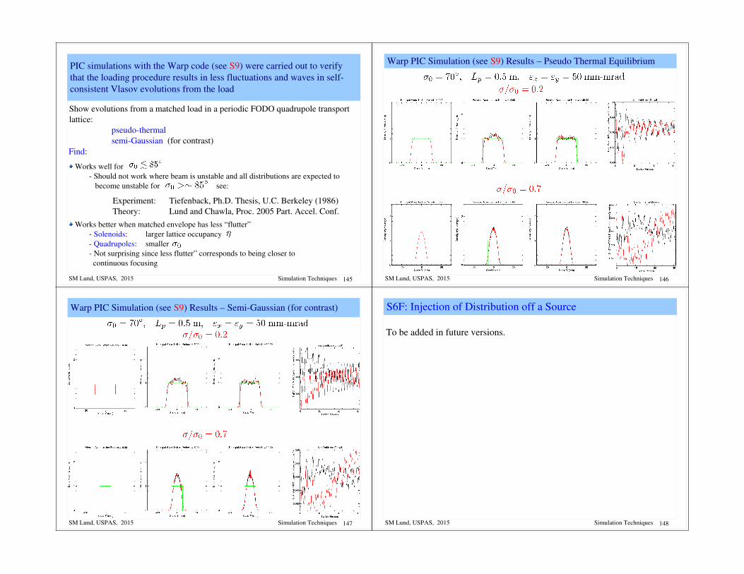
PIC simulations with the Warp code (see S9) were carried out to verify that the loading procedure results in less fluctuations and waves in selfconsistent Vlasov evolutions from the load
Show evolutions from a matched load in a periodic FODO quadrupole transport lattice:
pseudothermal semiGaussian (for contrast)
Find:
Works well for Should not work where beam is unstable and all distributions are expected to become unstable for see:
Works better when matched envelope has less “flutter” Solenoids: larger lattice occupancy Quadrupoles: smaller Not surprising since less flutter” corresponds to being closer to continuous focusing
Experiment: Tiefenback, Ph.D. Thesis, U.C. Berkeley (1986)Theory: Lund and Chawla, Proc. 2005 Part. Accel. Conf.
SM Lund, USPAS, 2015 146Simulation Techniques
Warp PIC Simulation (see S9) Results – Pseudo Thermal Equilibrium
SM Lund, USPAS, 2015 147Simulation Techniques
Warp PIC Simulation (see S9) Results – SemiGaussian (for contrast)
SM Lund, USPAS, 2015 148Simulation Techniques
S6F: Injection of Distribution off a Source
To be added in future versions.
SM Lund, USPAS, 2015 149Simulation Techniques
S7: Numerical ConvergenceS7A: Overview
Numerical simulations must be checked for proper resolution and statistics to be confident that answers obtained are correct and physical:
Resolution of discretized quantitiesTime t or axial s step of advanceSpatial grid of fieldsolveFor direct Vlasov: the phasespace grid
Statistics for PICNumber of macroparticles used to represent Vlasov flow to control noise
Increased resolution and statistics generally require more computer resources (time and memory) to carry out the required simulation. It is usually desirable to carry out simulations with the minimum resources required to achieve correct, converged results that are being analyzed. Unfortunately, there are no set rules on adequate resolution and statistics. What is required generally depends on:
What quantity is of interestHow long an advance is required What numerical methods are being employed .....
SM Lund, USPAS, 2015 150Simulation Techniques
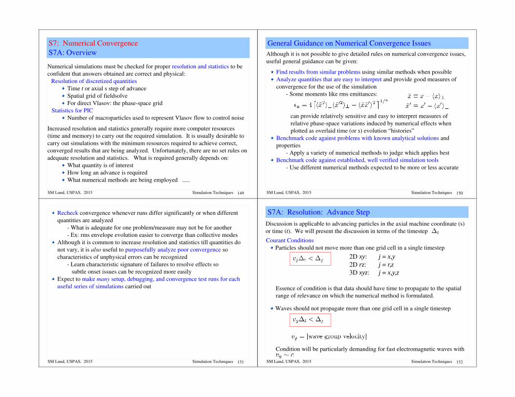
General Guidance on Numerical Convergence IssuesAlthough it is not possible to give detailed rules on numerical convergence issues, useful general guidance can be given:
Find results from similar problems using similar methods when possibleAnalyze quantities that are easy to interpret and provide good measures of convergence for the use of the simulation
Some moments like rms emittances:
can provide relatively sensitive and easy to interpret measures of relative phasespace variations induced by numerical effects when plotted as overlaid time (or s) evolution “histories”
Benchmark code against problems with known analytical solutions and properties
Apply a variety of numerical methods to judge which applies bestBenchmark code against established, well verified simulation tools
Use different numerical methods expected to be more or less accurate
SM Lund, USPAS, 2015 151Simulation Techniques
Recheck convergence whenever runs differ significantly or when different quantities are analyzed
What is adequate for one problem/measure may not be for another Ex: rms envelope evolution easier to converge than collective modes
Although it is common to increase resolution and statistics till quantities do not vary, it is also useful to purposefully analyze poor convergence so characteristics of unphysical errors can be recognized
Learn characteristic signature of failures to resolve effects so subtle onset issues can be recognized more easily
Expect to make many setup, debugging, and convergence test runs for each useful series of simulations carried out
SM Lund, USPAS, 2015 152Simulation Techniques
S7A: Resolution: Advance StepDiscussion is applicable to advancing particles in the axial machine coordinate (s) or time (t). We will present the discussion in terms of the timestep
Courant ConditionsParticles should not move more than one grid cell in a single timestep
Essence of condition is that data should have time to propagate to the spatial range of relevance on which the numerical method is formulated.
Waves should not propagate more than one grid cell in a single timestep
Condition will be particularly demanding for fast electromagnetic waves with
2D xy: j = x,y 2D rz: j = r,z3D xyz: j = x,y,z
SM Lund, USPAS, 2015 153Simulation Techniques
Resolution of Applied Field StructuresEnough steps should be taken to adequately resolve applied field structures
SM Lund, USPAS, 2015 154Simulation Techniques
Variation of collective oscillations (waves)For a leapfrog mover this requires minimally
Collective modes can have high harmonic components which evolve rapidly rending resolution issues difficult. See lectures on Transverse Kinetic Stability
SM Lund, USPAS, 2015 155Simulation Techniques
S7C: Resolution: Spatial GridThe spatial grid should resolve both spacecharge variations of the beam associated with both the bulk structure of the beam and collective waves
Beam EdgeEstimate from equilibrium beam properties (see lectures on Transverse Equilibrium Distributions) as being on the scale of the characteristic thermal Debye length
SM Lund, USPAS, 2015 156Simulation Techniques
S7D: Statistics Collective effects require having a significant number of particles within the “volume” bounded by the characteristic shielding distance
Shielding distance given by the Debye length:
“Volume” bounded by shielding distance will depend on the dimension of the simulation being carried out. For simulations with N macroparticles:

SM Lund, USPAS, 2015 157Simulation Techniques
S7E: Illustrative Examples with the Warp Code
SM Lund, USPAS, 2015 158Simulation Techniques
Example: Weak SpaceCharge Case; rms Envelope
SM Lund, USPAS, 2015 159Simulation Techniques
S8: Practical Considerations:A: Overview
Intense beam simulation problems can be highly demanding on computer resources – particularly for realistic higher dimensional models. The problem size that can be simulated is dictated by computer resources available in fast memory and the run time required to complete the simulation
Fast Memory (RAM)Wall Clock Run Time (Computer Speed)
Both of these can depend strongly on the architecture of computer system that the problem is run on:
Serial MachineParallel Machine
can strongly influence the size of the problem that can be simulated. We will present rough estimates of the computer memory required for simulations and provide some guidance on how the total simulation time can scale on various computer systems. The discussion is limited to PIC and direct Vlasov simulations.
SM Lund, USPAS, 2015 160Simulation Techniques
S8B: Practical Considerations: Fast Memory
Fast computer memory (RAM) dictates how large a problem can be simulatedIf a problem will not fit into fast memory (RAM), computer performance will be severely compromisedWrites to hard disks are slow
There are 3 main contributions to the problem size for typical PIC or direct Vlasov simulations:
1) Particle Phase Space Coordinates (PIC) or Discretized Distribution Function (Direct Vlasov)2) Gridded Field3) General Code Overhead
These three contributions to memory required are discussed in turn
Particle and field quantities are typically stored in double precision:
Single PrecisionDouble Precision
Representation Digits (Floating Point) Bytes Memory 816
48Most
problems

SM Lund, USPAS, 2015 161Simulation Techniques
Estimates of Required Fast Memory1) Particle Phase Space Coordinates (PIC):
Memory = B * Np * D Bytes
B = bytes of floating point number (typically 8 for double precision)N
p = number macro particles (0 for direct Vlasov)
D = dimension of variables characterizing particles
The dimension D depends on the specific type of PIC simulation and methods employed// Common Examples of D:
3D PIC: D = 7 2D Transverse Slice PIC: D = 5
//
+ (D=6) some models
is often included often to optimize the mover
SM Lund, USPAS, 2015 162Simulation Techniques
Estimates of Required Fast Memory1) Discretized Distribution Function (Direct Vlasov):
Memory = B * Npm
Bytes
B = bytes of floating point number (typically 8 for double precision)N
pm = number mesh points of grid describing the discretized
particle phase space
The value of Npm
depends critically on the dimensionality of the phase space
// Examples of Npm
scaling for a uniform phasespace meshes:
Rapid growth of Npm
with dimensionality severely limits mesh size
SM Lund, USPAS, 2015 163Simulation Techniques
//
Memory required for a double precision (B = 8) uniform phasespace grid with 100 zone discretization per degree of freedom:
Rapidly increasing problem size with phasespace dimension D practically limits what can be simulated on direct Vlasov simulations with reasonable resolution even on large parallel computers:
Irregular phasespace grids that place resolution where it is needed can partially alleviate scaling problem: provides more help in higher dimensionsImproved methods also seek to only grid minimal space exterior to the oscillating beam core in alternating gradient lattices
SM Lund, USPAS, 2015 164Simulation Techniques
2) Gridded Field:Required memory for a gridded field solve depends on the class of field solve (electrostatic, electromagnetic), mesh size, and numerical method employed. For a concrete illustration, consider electrostatic problems using a simple FFT field solve:
Discrete Fourier Transform complex, but transform is of real functions. Optimization allows use of transforms using only real and arraysElectric field is typically not stored and is calculated for each particle only where it is needed. Spatial grid location need not be stored. Some methods store gridded E to optimize specific problems
Memory = 2 * B* Nfm
Bytes
Nfm
= number mesh points of field spatial grid
Factor of 2 for:

SM Lund, USPAS, 2015 165Simulation Techniques
Number of mesh points Nfm
depends strongly on the dimensionality of the field
solve and the structure of the meshGenerally more critical to optimize storage and efficiency (see next section) of fieldsolvers in higher dimensions
Examples for uniform meshes:
1D (Longitudinal)
2D (Transverse Slice)
3D2D (rz Axisymmetric)
SM Lund, USPAS, 2015 166Simulation Techniques
3) General Code Overhead:System memory is also used for:
Scratch arrays for various numerical methods (fieldsolvers, movers, etc.)History accumulations of diagnostic momentsDiagnostic routinesGraphics packages, external libraries, etc.
Graphics packages can be large!
Summary: Total Memory Required:
For illustrative example, add memory contributions for electrostatic PIC
PIC: Total Memory = B * ( Np * D + 2 * N
fm ) + M
overheadBytes
Direct Valsov: Total Memory = 2 * B * ( Npm
+ Nfm
) + Moverhead
Bytes
Memory = Moverhead
Bytes
Characteristic of packages used, size of code, and methods employed. But typical numbers can range 1 MB – 20 MBytes
Reminder: Machine fast memory (RAM) capacity should not be exceededStoring data on disk and cycling to RAM generally too slow!
SM Lund, USPAS, 2015 167Simulation Techniques
S8C: Practical Considerations: Run Time
Run time can depend on many factors including:Type of problem Dimensionality of problem and number of particles and/or mesh points Numerical methods employed (particle moving, fieldsolve, ....)Moments and diagnostics accumulatedArchitecture/speed of computer system
It is not possible to give fully general guidance on estimating run times. However, to better characterize the time required, it can be useful to benchmark the code on the computer to be employed in terms of:
tstep
= Time for an “ordinary” run step
Generally, parts of the code that more time is spent in should be more carefully optimized to minimize total run time. Particular care should be taken with:
Particle mover Field solver Frequent computationally intense diagnostics such as moments
SM Lund, USPAS, 2015 168Simulation Techniques
Diagnostics, loaders, problem setup routines, etc. can often be coded with less care for optimization since they are only executed infrequently. However:
Diagnostics often take a large amount of development time Often better to code as simply as possible to avoid problems!
Software profiling tools can be useful to best understand where “bottlenecks” occur so effort on optimization can be appropriately directed for significant returns.

SM Lund, USPAS, 2015 169Simulation Techniques
Some general guidance for electrostatic PIC Simulations:
1D: (Longitudinal typical)Fieldsolve generally fast: small fraction of time compared to moving particles
Green's function methods can be used (Gauss Law)
2D: (Transverse xy slice and axisymmetric rz typical)Fieldsolve typically a small fraction of time relative to moving particles if fast gridded methods are applied (like FFT based methods)
Special boundary conditions can increase the fraction
Dimensionality plays a strong role in required run time
Method Numerical WorkFFT with Periodic BC Small fraction of particle movingFFT with Capacity Matrix .Multigrid .. .Green's Function Dominates particle moving
SM Lund, USPAS, 2015 170Simulation Techniques
3D:Fieldsolve typically comparable in time or dominates time for particle moving even if fast, gridded methods are applied
Fieldsolve efficiency of critical importance in 3D to optimize run timeWhole classes can be taught just on methods of 3D electrostatic field solves for the Poisson equation discretized on a mesh
Some general guidance for Direct Vlasov Simulations:
The rapid growth of the problem size with the phase spacedimension and available fast computer memory can severely limit problem sizes that can be simulated:
Numerical work can be significant to advance the discretized distribution over characteristics Size of gridded field arrays can be very large leading to slow advances Nonuniform mesh can help control size at the expense of code complexity
SM Lund, USPAS, 2015 171Simulation Techniques
The type of computer system employed can also strongly influence run time Processor Speed Memory Speed
RAM Fast, optimized cache memory
System Architecture (see next section) Serial Parallel
Library Optimization Especially relevant for parallel machines
SM Lund, USPAS, 2015 172Simulation Techniques
S8D: Practical Considerations: Machine Architectures
Problems may be simulated on: 1) Serial Machines
Single processor or an independently run processor on a multiprocessor machine (example: most present multi”core” processors)
2) Parallel MachineMultiprocessors coordinated to work as a large single processor Usually employ independent memory for each processor making up the machine but sometimes uses shared memory among processors
Serial machines represent traditional computers (PCs, workstations, etc), whereas parallel machines are generally less familiar.
Overview of parallel simulations:
In recent years parallel machines have significantly improved with libraries that allow more “natural” problem formulation with less effort. This is enabling significantly larger simulations to be carried out
Several 100 million particles typically practical to simulate on large machines with fast, gridded fieldsolve

SM Lund, USPAS, 2015 173Simulation Techniques
Beam problems may often be conveniently partitioned among processors in terms of axial slices. Schematic example (5 processors):
Typical Parallel Machine Architecture
Sharing of data at boundaries is necessary for fieldsolve in electrostatic caseProblems with axial velocity spread generally requires sorting of particles to maintain the load balance between processors
Processors should ideally all perform an equal amount of work since the slowest will dictate the total time of the advance step
par_partition.png
SM Lund, USPAS, 2015 174Simulation Techniques
Ideal parallelization results in a linear speedup with processor numberActual speedup typically less due to:
Overhead in data transfers Lack of ideal load balance causing processors to wait on the slowest one that the problem is partitioned among
par_speedup.eps
SM Lund, USPAS, 2015 175Simulation Techniques
Even with the significant advances in problem size and speed promised by parallel computers, the solution of realistic 3D beam problems with direct (not gridded) fields remains far too large a problem to simulate with present computer systems. Also, the continuum limit Vlasov solution to problems is in itself of intrinsic interest as a well posed model of many physical systems. Thus, for detailed simulations, we often push computer resources to the maximum extent possible.
Better numerical algorithmsParallelization....
SM Lund, USPAS, 2015 176Simulation Techniques
S9: Warp Code Overview
See the Warp web site: http://warp.lbl.gov

SM Lund, USPAS, 2015 177Simulation Techniques
S10: Example Simulations
Examples to this point have mostly been simply formulated to illustrate concepts. Here, we present results from more complex simulations carried out in support of experiments, theory, and for machine design. Simulations highlighted include:
Electrostatic Quadrupole Injector Multibeamlet Injector Collective Mode Effects Detailed Transport Lattice DesignTransport Limits in Periodic Quadrupole Focusing ChannelsElectron Cloud Effects for Ion Beam Transport
All these simulations, as well as many of the preceding illustrations in the lecture notes, were produced with the Warp code described in S9. Only select issues from the problems are highlighted.
SM Lund, USPAS, 2015 178Simulation Techniques
Example: Electrostatic Quadrupole Injector
See handwritten notes from USPAS 06 for remaining slidesWill be updated in future versions of the notes
SM Lund, USPAS, 2015 179Simulation Techniques
Corrections and suggestions for improvements welcome!
These notes will be corrected and expanded for reference and for use in future editions of US Particle Accelerator School (USPAS) and Michigan State University (MSU) courses. Contact:
Prof. Steven M. Lund Facility for Rare Isotope Beams Michigan State University 640 South Shaw Lane East Lansing, MI 48824
[email protected] (517) 908 – 7291 office (510) 459 4045 mobile
Please provide corrections with respect to the present archived version at: https://people.nscl.msu.edu/~lund/uspas/bpisc_2015
Redistributions of class material welcome. Please do not remove author credits.SM Lund, USPAS, 2015 180Simulation Techniques
References: For more information see: These course notes are posted with updates, corrections, and supplemental material at:
https://people.nscl.msu.edu/~lund/uspas/bpisc_2015Materials associated with previous and related versions of this course are archived at:
JJ Barnard and SM Lund, Beam Physics with Intense SpaceCharge, USPAS:http://hifweb.lbl.gov/USPAS_2011 2011 Lecture Notes + Infohttps://people.nscl.msu.edu/~lund/uspas/bpisc_2011/
http://uspas.fnal.gov/programs/pastprograms.shtml (2008, 2006, 2004) JJ Barnard and SM Lund, Interaction of Intense Charged Particle Beams with Electric and Magnetic Fields, UC Berkeley, Nuclear Engineering NE290H
http://hifweb.lbl.gov/NE290H 2009 Lecture Notes + Info

SM Lund, USPAS, 2015 181Simulation Techniques
References: Continued (2):
Numerical MethodsForman S. Acton, Numerical Methods that Work, Harper and Row Publishers, New York (1970)
Steven E. Koonin, Computational Physics, AddisonWesley Publishing Company (1986)
W. Press, B. Flannery, S. Teukolsky, W. Vetterling, Numerical Recipes in C: The Art of Scientific Computing, Cambridge University Press (1992)
Particle MethodsC.K. Birdsall and A.B. Langdon, Plasma Physics via Computer Simulation, McGrawHill Book Company (1985)
R.W. Hockney and J.W. Eastwood, Computer Simulation using Particles, Institute of Physics Publishing (1988)
Review of Initial Distribution LoadsS. Lund, T. Kikuchi, and R. Davidson, “Generation of initial kinetic distributions for simulation of longpulse charged particle beams with high spacecharge intensity,” PRSTAB 12, 114801 (2009)
SM Lund, USPAS, 2015 182Simulation Techniques
Acknowledgments: These lecture notes reflect input from numerous scientists and engineers who helped educate the author in accelerator physics over many years. Support enabling the long hours it took to produce these lecture notes were provided by the Facility for Rare Isotope Beams (FRIB) at Michigan State University (MSU), Lawrence Livermore National Laboratory (LLNL), and Lawrence Berkeley National Laboratory (LBNL). Special thanks are deserved to:
Rodger Bangerter Martin Berz John Barnard Oliver BoineFrankenheim Richard Briggs Ronald DavidsonMikhail Dorf Andy Faltens Bill Fawley Giuliano Franchetti Alex Friedman Dave Grote Irving Haber Klaus HalbachEnrique Henestroza Ingo Hoffmann Dave JuddIgor Kagonovich Takashi Kikuchi Rami Kishek Joe KwanEd Lee Daniela Leitner Steve Lidia Guillaume Machicoane Felix Marti Hiromi OkamotoEduard Pozdeyez Martin Reiser Lou Reginato Robert RyneGianLuca Sabbi Peter Seidl William Sharp Peter Spiller Edward Startsev Ken Takayama JeanLuc Vay Will WaldronTom Wangler Jie Wei Yoshi Yamazaki Simon YuPavel Zenkovich Yan Zhang Qiang Zhao
SM Lund, USPAS, 2015 183Simulation Techniques
Special thanks are deserved for Alex Friedman, Dave Grote, and JeanLuc Vay of the Lawrence Livermore and Lawrence Berkeley National Laboratories for help with these notes and extensively educating the author in simulation methods.
Sven Chilton (UCB, LLNL) assisted in the development of part of these lecture notes and in generating some of the numerical examples and figures
Kei Fukushima, (Hiroshima U), Kazuya Osaki (Hiroshima U), Jonathan Wong (U. Hong Kong), and Albert Yuen (UCB) all attended an informal version of a simulation course based on these notes at LBNL in 2012 which resulted in numerous improvements in material.
Rami Kishek (UMD) assisted teaching a version of this course and contributed to the simulation notes.
Irving Haber (UMD) helped educate the author on various simulation methods.
Michiel de Hoon helped with an early version of the lectures and with example Lagrangian methods.
Acknowledgments Continued: