simulation study of conwip for a cold rolling plant

Int. J. Production Economics 54 (1998) 257—266

Simulation study of CONWIP for a cold rolling plant

Min Huang!,*, Dingwei Wang!, W.H. Ip"

! Department of Systems Engineering, Box 135, College of Information Science and Engineering, Northeastern University, Shenyang, 110006,Liaoning, People+s Republic of China

" Department of Manufacturing Engineering, Hong Kong Polytechnic University, Kowloon, Hong Kong

Received 10 March 1997; accepted 20 November 1997

Abstract

The CONWIP production control system has received a great deal of attention from researchers recently. In thispaper, we introduce a method to determine the card number of the CONWIP system for a production line witha bottleneck. The simulation study compares the CONWIP system and the original control system for the four situationsin a cold rolling plant. Simulation results show that the CONWIP production control system is very efficient for theproduction and inventory control of semi-continuous manufacturing, such as that found in the steel rolling plant. It cangreatly reduce the work-in-process (WIP), decrease the average inventory and average inventory costs, and guaranteea higher throughput rate and facility utilization. ( 1998 Elsevier Science B.V. All rights reserved.

Keywords: Production control system; Simulation; Just-in-time; MRP-II; CONWIP; Kanban system

1. Introduction

Effective production control systems are thosethat produce the right parts, at the right time, ata competitive cost. Production control systems cangenerally be divided into push and pull systems [1].The best known push systems are materials re-quirements planning (MRP) and its successormanufacturing resources planning (MRP-II), bothdeveloped in western countries. The best knownpull system is kanban, which was developed inJapan [2].

In a push system, production is controlled bya central planning system, that takes load forecasts

*Corresponding author. E-mail: [email protected].

as future demands. Production is initiated beforethe occurrence of demand, otherwise the goodscannot be delivered in time. Therefore, the produc-tion lead times have to be known or approximated.

In a pull system, production is triggered by theactual demand. The production is initiated by a de-centralized control system. To avoid long waitingtimes for customers, parts and finished productsmust be stored in buffers [3].

Both push system and pull system have differentadvantages and disadvantages, as has been pointedout by many researchers [1,4,5]. MRP is generallyconsidered to be applicable to many more manu-facturing environments than kanban. However,kanban seems to produce superior results wheneverit is applied [1]. Therefore, many researchers try tocombine the two types of control systems [6—8].

0925-5273/98/$19.00 Copyright ( 1998 Elsevier Science B.V. All rights reservedPII S 0 9 2 5 - 5 2 7 3 ( 9 7 ) 0 0 1 5 2 - 7

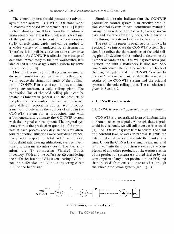
Fig. 1. The CONWIP system.

The control system should possess the advant-ages of both systems. CONWIP (CONstant WorkIn Process) proposed by Spearman et al. [1] is justsuch a hybrid system. It has drawn the attention ofmany researchers. It has the substantial advantagesof the pull system is to control work-in-process(WIP) directly using cards, and can be applied toa wider variety of manufacturing environments.Therefore, it is a pull-based system as an alternativeto kanban. As CONWIP feedbacks the message ofdemands immediately to the first workcenter, it isalso called a single-stage kanban system by someresearchers [1,9,10].

Most push systems and pull systems are used indiscrete manufacturing environment. In this paperwe introduce the simulation study of the applica-tion of CONWIP in a semi-continuous manufac-turing environment, a cold rolling plant. Theproduction line of the cold rolling plant can betreated as tandem in general, and the products ofthe plant can be classified into two groups whichhave different processing routes. We introducea method to determine the number of cards in theCONWIP system for a production line witha bottleneck, and compare the CONWIP systemwith the original control system. The original sys-tem controls the production quantity of the prod-ucts at each process each day. In the simulation,four production situations were considered respec-tively with respect to total WIP, input rate,throughput rate, average utilization, average inven-tory and average inventory costs. The four situ-ations are (1) considering Finished GoodsInventory (FGI) and the buffer size, (2) consideringthe buffer size but not FGI, (3) considering FGI butnot the buffer size, and (4) not considering eitherFGI or the buffer size.

Simulation results indicate that the CONWIPproduction control system is an effective produc-tion control system in semi-continuous manufac-turing. It can reduce the total WIP, average inven-tory and average inventory costs, while ensuringhigh throughput rate and average facility utilization.

The rest of the paper is organized as follows. InSection 2, we introduce the CONWIP system. Sec-tion 3 describes the characteristics of the cold roll-ing plant. In Section 4, the method to determine thenumber of cards in the CONWIP system for a pro-duction line with a bottleneck is discussed. Sec-tion 5 introduces the control mechanism both ofthe original system and the CONWIP system. InSection 6, we compare and analyze the simulationresults of the CONWIP system and the originalsystem in the cold rolling plant. The conclusion isgiven in Section 7.

2. CONWIP control system

2.1. CONWIP production/inventory control strategy

CONWIP is a generalized form of kanban. Likekanban, it relies on signals. Although these signalscould be electronic, we will call them cards as usual[1]. The CONWIP system tries to control the plantat a constant level of work in process. It limits thetotal number of parts allowed into the plant at anytime. Under the CONWIP system, the raw materialis “pulled” into the production system by the com-pletion of any other products at the output stationof the production systems (saturated line) or by theconsumption of any other products in the FGI, andthen “pushed” from one station to another throughthe whole production system (see Fig. 1).

258 M. Huang et al. /Int. J. Production Economics 54 (1998) 257—266

Like the kanban system, the CONWIP systemonly responds to the actual demands of customers,so it is a pull-based system, and some researchershave pointed out that the CONWIP system isa single-stage kanban system [1,9,10].

2.2. Advantages of the CONWIP system

As pull systems, the CONWIP system and thekanban system have some common advantagesover push systems.

1. Pull systems have lower WIP and this has theadvantage of making any problems in the plantmore obvious.

2. Pull systems can be modeled as a closed queue-ing network, on the other hand, push systemscan be modeled as an open queueing network.As such, the WIP, average flow time and vari-ance of flow time in pull systems tend to be lessthan that of push systems.

3. Pull systems are easy to control, because pullsystems control WIP, while push systems con-trol throughput.

CONWIP also has some unique advantages thatare superior to push systems.

1. CONWIP is superior to push systems when theproduction system runs under the highest pos-sible throughput rates.

2. CONWIP also appears to alleviate a problemfound in many push systems called “overtimevicious cycle”.

As the alternative to kanban, the CONWIP sys-tem has some superior characteristics over the kan-ban system [1,11].

1. CONWIP is more general than the kanban sys-tem. It is applicable to production environmentswhich produce many kinds of products.

2. CONWIP makes no attempt to control the loca-tion of the WIP within the system.

3. Although some researchers have shown thata kanban system would have lower WIP levels

than a CONWIP system with the same through-put under some certain conditions [3], mostresearchers have pointed out that CONWIPwould result in lower WIP levels than a kanbansystem with the same throughput in most cases[1,11].

In short, if kanban is good, CONWIP is better.

3. Characteristics of the cold rolling plant

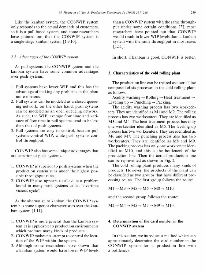
The production line can be treated as a serial linecomposed of six processes in the cold rolling plantas follows:

Acidity washingPRollingPHeat treatmentPLeveling upPPunchingPPacking.

The acidity washing process has two workcen-ters. They are identified as M1 and M2. The rollingprocess has two workcenters. They are identified asM3 and M4. The heat treatment process has onlyone workcenter identified as M5. The leveling upprocess has two workcenters. They are identified asM6 and M7. The punching process also has twoworkcenters. They are identified as M8 and M9.The packing process has only one workcenter iden-tified as M10, and this is the bottleneck of theproduction line. Then the actual production linecan be represented as shown in Fig. 2.

The cold rolling plant produces many kinds ofproducts. However, the products of the plant canbe classified as two groups that have different pro-cessing routes. The first group follows the route:

M1PM3PM5PM6PM8PM10;

and the second group follows the route:

M2PM4PM5PM7PM9PM10.

4. Determination of the card number in theCONWIP system

In this section, we introduce a method which canapproximately determine the card number in theCONWIP system for a production line witha bottleneck.

M. Huang et al. /Int. J. Production Economics 54 (1998) 257—266 259

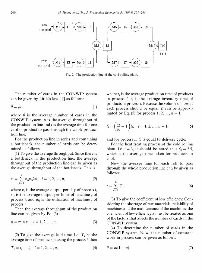
Fig. 2. The production line of the cold rolling plant.

The number of cards in the CONWIP systemcan be given by Little’s law [1] as follows:

h"kt, (1)

where h is the average number of cards in theCONWIP system, k is the average throughput ofthe production line and t is the average time for onecard of product to pass through the whole produc-tion line.

For the production line in series and containinga bottleneck, the number of cards can be deter-mined as follows:

(1) To give the average throughput: Since there isa bottleneck in the production line, the averagethroughput of the production line can be given asthe average throughput of the bottleneck. This is

vi"

n+j/1

vijuij24, i"1, 2,2, n, (2)

where viis the average output per day of process i,

vij

is the average output per hour of machine j ofprocess i, and u

ijis the utilization of machine j of

process i.Then the average throughput of the production

line can be given by Eq. (3).

k"min vi, i"1, 2,2, n. (3)

(2) To give the average lead time: Let ¹ibe the

average time of products passing the process i, then

¹i"t

i#t@

i, i"1, 2,2, n, (4)

where tiis the average production time of products

in process i, t@i

is the average inventory time ofproducts in process i. Because the volume of flow ateach process should be equal, t@

ican be approxi-

mated by Eq. (5) for process 1, 2,2, n!1,

t@i"A

vi

ki

!1B ti, i"1, 2,2, n!1, (5)

and for process n, t@n

is equal to delivery cycle.For the heat treating process of the cold rolling

plant, i.e. i"3, it should be noted that t@3"2.5,

which is the average time taken for products tocool.

Now the average time for each roll to passthrough the whole production line can be given asfollows:

t"6+i/1

¹i. (6)

(3) To give the coefficient of low efficiency: Con-sidering the shortage of raw materials, reliability ofmachines and the maintenance of the machines, thecoefficient of low efficiency x must be treated as oneof the factors that affects the number of cards in theCONWIP system.

(4) To determine the number of cards in theCONWIP system: Now, the number of constantwork in process can be given as follows:

h"kt(1#x) . (7)


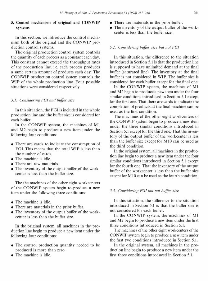
5. Control mechanism of original and CONWIPsystems

In this section, we introduce the control mecha-nism both of the original and the CONWIP pro-duction control systems.

The original production control system controlsthe quantity of each process as a constant each day.This constant cannot exceed the throughput ratesof the production line. i.e. each process producesa same certain amount of products each day. TheCONWIP production control system controls theWIP of the whole production line. Four possiblesituations were considered respectively.

5.1. Considering FGI and buffer size

In this situation, the FGI is included in the wholeproduction line and the buffer size is considered foreach buffer.

In the CONWIP system, the machines of M1and M2 begin to produce a new item under thefollowing four conditions:

f There are cards to indicate the consumption ofFGI. This means that the total WIP is less thanthe number of cards.

f The machine is idle.f There are raw materials.f The inventory of the output buffer of the work-

center is less than the buffer size.

The the machines of the other eight workcentersof the CONWIP system begin to produce a newitem under the following three conditions:

f The machine is idle.f There are materials in the prior buffer.f The inventory of the output buffer of the work-


In the original system, all machines in the pro-duction line begin to produce a new item under thefollowing four conditions:

f The control production quantity needed to beproduced is more than zero.

f The machine is idle.

f There are materials in the prior buffer.f The inventory of the output buffer of the work-


5.2. Considering buffer size but not FGI

In this situation, the difference to the situationintroduced in Section 5.1 is that the production lineis supposed to have unlimited demand at the finalbuffer (saturated line). The inventory at the finalbuffer is not considered in WIP. The buffer size isconsidered for each buffer except for the final one.

In the CONWIP system, the machines of M1and M2 begin to produce a new item under the foursimilar conditions introduced in Section 5.1 exceptfor the first one. That there are cards to indicate thecompletion of products at the final machine can beused as the first condition.

The machines of the other eight workcenters ofthe CONWIP system begin to produce a new itemunder the three similar conditions introduced inSection 5.1 except for the third one. That the inven-tory of the output buffer of the workcenter is lessthan the buffer size except for M10 can be used asthe third condition.

In the original system, all machines in the produc-tion line begin to produce a new item under the foursimilar conditions introduced in Section 5.1 exceptfor the fourth one. That the inventory of the outputbuffer of the workcenter is less than the buffer sizeexcept for M10 can be used as the fourth condition.

5.3. Considering FGI but not buffer size

In this situation, the difference to the situationintroduced in Section 5.1 is that the buffer size isnot considered for each buffer.

In the CONWIP system, the machines of M1and M2 begin to produce a new item under the firstthree conditions introduced in Section 5.1.

The machines of the other eight workcenters of theCONWIP system begin to produce a new item underthe first two conditions introduced in Section 5.1.

In the original system, all machines in the pro-duction line begin to produce a new item under thefirst three conditions introduced in Section 5.1.


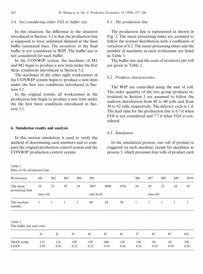
Table 2The buffer size and costs

I1 I2 I3 I4 I5 I6 I7 I8 I9 I10

IMAX (rolls) 125 125 150 150 400 150 150 50 50 350COST 0.10 0.10 0.12 0.12 0.14 0.16 0.16 0.18 0.18 0.20

Table 1Data of the production line

Workcentre M1 M2 M3 M4 M5 M6 M7 M8 M9 M10

The meanprocessing time

24 22 18 36 3667 8000 4762 24 24 22 34 16

min/roll min/4roll min/roll

The machinenumber

1 1 1 1 40 24 36 1 1 1 1 1

5.4. Not considering either FGI or buffer size

In this situation, the difference to the situationintroduced in Section 5.1 is that the production lineis supposed to have unlimited demand at the finalbuffer (saturated line). The inventory at the finalbuffer is not considered in WIP. The buffer size isnot considered for each buffer.

In the CONWIP system, the machines of M1and M2 begin to produce a new item under the firstthree conditions introduced in Section 5.2.

The machines of the other eight workcenters ofthe CONWIP system begin to produce a new itemunder the first two conditions introduced in Sec-tion 5.1.

In the original system, all workcenters in theproduction line begin to produce a new item underthe the first three conditions introduced in Sec-tion 5.1.

6. Simulation results and analysis

In this section simulation is used to verify themethod of determining card numbers and to com-pare the original production control system and theCONWIP production control system.

6.1. The production line

The production line is represented as shown inFig. 2. The mean processing times are assumed tofollow the normal distribution with a coefficient ofvariation of 0.2. The mean processing times and thenumber of machines in each workcenter are listedin Table 1.

The buffer size and the costs of inventory per rollare given in Table 2.

6.2. Products characteristics

The WIP are controlled using the unit of roll.The order quantity of the two group products in-troduced in Section 3 are assumed to follow theuniform distribution from 48 to 60 rolls and from30 to 42 rolls, respectively. The delivery cycle is 1 d.The lead time for the production line is 6.7 d whenFGI is not considered and 7.7 d when FGI is con-sidered.

6.3. Simulation

In the simulation process, one roll of product istriggered on each machine, except for machines atprocess 3, which processes four rolls of product each


time. For the four situations introduced in Section 5,the product begins working at different times.

For the situation of considering FGI and buffersize, according to the control mechanism introduc-ed in Section 5, the time at which the jth productbegins at machine i in the CONWIP system can begiven as

¹(i, j)"GmaxMTC,¹(i, j!1)#S(i, j!1), TR

i,

TINiN, i"1, 2, j"1, 2,2,

maxM¹(i, j!1)#S(i, j!1), TIPi,

TINiN, iO1, 2, j"1, 2,2,

(8)

where TC is the time that the number of free cardsis not equal to zero last, S(i, j!1) is the processtime of product j!1 at machine i, TR

iis the time

that the raw buffer of machine i is not empty last,TIN

iis the time that the buffer of machine i is not

full last, TIPiis the time that the buffer prior to

machine i is not empty last.The time at which the jth product begin at ma-

chine i in the original system can be given as

¹(i, j)"maxMTQk,¹(i, j!1)

#S(i, j!1), TIPi, TIN

iN,

i"1, 2,2, 10, j"1, 2, k"1, 2,2, 6, (9)

where TQkis the time that the control production

quantity is not equal to zero last at the kth process.For the other three situations, the equation can

be given similarly.The simulation runs were undertaken for four

years. The first two years were ignored in analysisin order to reduce transient effects. The simulationsoftware was programmed in C language and thesimulation was performed on a PC/586. The dataused in simulation were collected from actual pro-duction.

In the simulation, the following six performancemeasures were calculated and evaluated:

1. Average WIP, which is measured by the averagenumber of products (rolls) in the whole produc-tion line during the last two years of the simula-tion. This includes the products being processedon the machines and stored in the buffers.

WIP"

T+i/1

WIPi/¹,

where WIPiis the WIP at the end of day i, ¹ is

the number of days in the last two years.2. Input rate j, which is measured by the average

number of raw materials (rolls) being input intothe production line each day during the last twoyears of the simulation.

j"T+i/1

INi/¹,

where INiis the input of the production line in

day i, ¹ is the number of days in the last twoyears.

3. Throughput rate k, which is measured by theaverage number of products (rolls) produced perday during the last two years of the simulation.

k"T+i/1

Pi/¹,

where Piis the number of products produced in

day i, ¹ is the number of days in the last twoyears.

4. Average utilization u, which is measured as theaverage utilization of all machines in the pro-duction line. The utilization of each machine isdefined as the percentage of time the machine isbusy. A machine can be either busy, blocked orstarved.

u"An+i/1

(si/t)BNn,

where siis working time of the machine i, t is

effective simulation time, n is the number of themachine.

5. Average inventory I, which is measured by theaverage inventory of products in all buffers inthe production line (does not include products inprocessing) each day during the last two years ofthe simulation.

I"AT+j/1

n+i/1

IijBN¹,

where Iij

is the inventory of products in bufferi at the end of day j, n is the number of the buffer,¹ is the number of days in the last two years.


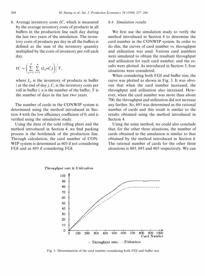
Fig. 3. Determination of the card number considering both FGI and buffer size.

6. Average inventory costs IC, which is measuredby the average inventory costs of products in allbuffers in the production line each day duringthe last two years of the simulation. The inven-tory costs of products per day in all the buffers isdefined as the sum of the inventory quantitymultiplied by the costs of inventory per roll eachday.

IC"AT+j/1

n+i/1

(Iij*

Ci)BN¹ ,

where Iij

is the inventory of products in bufferi at the end of day j, C

iis the inventory costs per

roll in buffer i, n is the number of the buffer, ¹ isthe number of days in the last two years.

The number of cards in the CONWIP system isdetermined using the method introduced in Sec-tion 4 with the low efficiency coefficient of 0, and isverified using the simulation study.

Using the data of the cold rolling plant and themethod introduced in Section 4, we find packingprocess is the bottleneck of the production line.Through calculation, the card number of CON-WIP system is determined as 603 if not consideringFGI and as 693 if considering FGI.

6.4. Simulation results

We first use the simulation study to verify themethod introduced in Section 4 to determine thecard number in the CONWIP system. In order todo this, the curves of card number vs. throughputand utilization was used. Various card numberswere simulated to obtain the resultant throughputand utilization for each card number, and the re-sults were plotted. As introduced in Section 5, foursituations were considered.

When considering both FGI and buffer size, thecurve was plotted as shown in Fig. 3. It was obvi-ous that when the card number increased, thethroughput and utilization also increased. How-ever, when the card number was more than about700, the throughput and utilization did not increaseany further. So, 693 was determined as the rationalnumber of cards and this result is similar to theresults obtained using the method introduced inSection 4.

Using the same method, we could also concludethat, for the other three situations, the number ofcards obtained in the simulation is similar to thatobtained by the method introduced in Section 4.The rational number of cards for the other threesituations is 603, 693 and 603 respectively. We can


Table 6Not considering either FGI or buffer size

WIP Utilization Inventory Cost Input Throughput

CONWIP 601 78.22 308 45.66 90 90Original 2826 77.44 2572 320.26 90 88

Table 5Considering FGI but not buffer size


CONWIP 693 78.47 404 65.13 90 90Original 2909 77.45 2655 336.67 90 88

Table 4Considering buffer size but not FGI


CONWIP 601 78.22 308 45.66 90 90Original 902 76.86 648 86.35 88 88

Table 3Considering FGI and buffer size


CONWIP 693 78.47 404 65.13 90 90Original 990 76.87 736 103.78 88 88

see that the method introduced in Section 4 isuseful for all the four situations.

We compared the CONWIP system with theoriginal system by simulation. For the four situ-ations, we recorded the performance measures in-troduced in Section 6.3 for both systems. TheCONWIP system was controlled using the rationalnumber of cards introduced above and the controlproduction quantity of the original system is 90rolls at each process each day.

Table 3 records the simulation result obtainedwhen considering FGI and buffer size. The CONWIPsystem has lower WIP, average inventory, averageinventory costs but higher utilization and through-put rates. This indicates that the CONWIP systemis superior to the original system in this situation.

Table 4 records the simulation result obtainedwhen considering buffer size but not FGI. TheCONWIP system also has lower WIP, averageinventory, average inventory costs but higher utiliz-ation and throughput rates. This indicates that theCONWIP system is superior to the original systemin this situation.

Table 5 records the simulation result obtainedwhen considering FGI but not buffer size. TheCONWIP system also has lower WIP, averageinventory, average inventory costs, but a higherutilization and throughput rates. Therefore, we canconclude that the CONWIP system is superior tothe original system in this situation.

Table 6 records the simulation result obtainedwhen not considering either FGI or buffer size. The


CONWIP system also has lower WIP, averageinventory, average inventory costs, but higher util-ization and throughput rates. Therefore, we canconclude that the CONWIP system is superior tothe original system in this situation.

We can see that the CONWIP system is superiorto the original system for all the four situations.There are two reasons for this. First, the CONWIPsystem has lower WIP, lower average inventoryand lower average inventory costs because it pro-duces products according to actual demands butthe original system produces products according toa certain constant. Second, the CONWIP systemhas higher utilization and throughput rates becauseonce the production of a product begins, the CON-WIP system produces the product as quickly aspossible, but the original system produces the prod-uct according to the control production quantityand this control production quantity limits the rateof the third process, the heat treatment process. Therate of the heat treatment process can only reach to88 rolls per day when the control productionquantity is 90 rolls per day, because the productionquantity of the heat treatment process must be themultiples of four rolls at any time as describedpreviously.

In addition to the results obtained above, an-other result worth noticing is that the input rate isequal to the throughput rate in the CONWIP sys-tem for all four situations.

7. Conclusions

In this paper, we first introduce a method todetermine the number of cards in the CONWIPsystem for a production line with a bottleneck, andthen use simulation to verify this method and com-pare the CONWIP system with the original systemin a type of semi-continuous manufacturing system,a cold rolling plant. The simulation study leads usto following conclusions.

1. The CONWIP system offers better perfor-mances than the original system. It has lowerWIP, higher throughput rate and utilization,while providing lower average inventory and

average inventory costs than those of the orig-inal system.

2. Input rate is equal to throughput rate in theCONWIP system. This proves the discussion ofSpearman et al., that, in a sense, CONWIP canbe considered as an input—output control [1].

Acknowledgements

The authors wish to thank an anonymous refereefor helpful comments. This work was partially sup-ported by the National High-Tech Program (863planning) of China, contract No. 863-511-9609-003,and the National Natural Science Foundation,contract No. 69684005.

References

[1] M.L. Spearman, D.L. Woodruff, W.J. Hoop, CONWIP:A pull alternative to Kanban, International Journal ofProduction Research 28 (5) (1990) 879—894.

[2] D. Wang, X. Chen, Y. Li, Experimental push/pull produc-tion planning and control system, Production Planningand Control 7 (3) (1996) 236—241.

[3] S. Gstettner, H. Kuhn, Analysis of production controlsystems kanban and CONWIP, International Journal ofProduction Research 34 (11) (1996) 3253—3273.

[4] J.L. Deleersnyder, T.J. Hodgson, H. Mueller(-Malek), P.J.O’Grady, Kanban controlled pull system: An analysis ap-proach, Management Science 35 (9) (1989) 1079—1091.

[5] B.R. Sarker, J.A. Fitzsimmons, The performance of pushand pull systems: a simulation and comparative study,International Journal of Production Research 27 (11)(1989) 1715—1732.

[6] S.D.P. Flapper, G.J. Miltenburg, J. Wijugard, EmbeddingJIT into MRP, International Journal of Production Re-search 29 (2) (1991) 329—341.

[7] N.E. Larsen, L. Alting, Criteria for selecting a productioncontrol philosophy, Production Planning and Control4 (1) (1993) 54—68.

[8] A. Villa, T. Watanabe, Production management: beyondthe dichotomy between ‘push’ and ‘pull’, Computer Integ-rated Manufacturing Systems 6 (1) (1993) 53—63.

[9] M.L. Spearman, Customer service in pull production sys-tems, Operations Research 40 (5) (1992) 948—958.

[10] M.D. Mascolo, Y. Frein, Y. Dalley, An analytical methodfor performance evaluation of kanban controlled produc-tion systems, Operations Research 44 (1) (1996) 50—64.

[11] M.L. Spearman, M.A. Zazanis, Push and pull productionsystems: issue and comparison, Operations Research 40 (3)(1992) 521—532.


simulation study of conwip for a cold rolling plant

Documents