simulation studies of a recorder in three dimensions

Simulation studies of a recorder in three dimensions

N. Giordanoa)

Department of Physics, Purdue University, West Lafayette, Indiana 47907

(Received 23 July 2013; revised 25 November 2013; accepted 12 December 2013)

The aeroacoustics of a recorder are explored using a direct numerical simulation based on the

Navier–Stokes equations in three dimensions. The qualitative behavior is studied using spatial

maps of the air pressure and velocity to give a detailed picture of jet dynamics and vortex shedding

near the labium. In certain cases, subtle but perhaps important differences in the motion of the air

jet near the edge of the channel as compared to the channel center are observed. These differences

may be important when analyzing experimental visualizations of jet motion. The quantitative

behavior is studied through analysis of the spectrum of the sound pressure outside the instrument.

The effect of chamfers and of changes in the position of the labium relative to the channel on the

tonal properties are explored and found to be especially important in the attack portion of the tone.

Changes in the spectrum as a result of variations in the blowing speed are also investigated as

well as the behavior of the spectrum when the dominant spectral component switches from the

fundamental to the second harmonic mode of the resonator tube.VC 2014 Acoustical Society of America. [http://dx.doi.org/10.1121/1.4861249]

PACS number(s): 43.75.Qr, 43.75.Zz, 43.75.Bc [TRM] Pages: 906–916

I. INTRODUCTION

In a recent paper,1 the author presented results of a study

of a two dimensional model of the recorder using numerical

solutions of the Navier–Stokes equations. In this paper, the

extension of that work to a fully three dimensional model of

the recorder is described. One goal is to use Navier–Stokes

based modeling to elucidate how the tonal properties of the

recorder and of the closely related case of a flue organ pipe

depend on the detailed geometry of the channel and labium.

We also explore the transition to higher notes as the blowing

speed is increased.

A broader goal of our work is to use Navier–Stokes

based modeling of a relatively simple wind instrument (the

recorder) to explore how specific features of the instrument

affect the quantitative tonal properties. In this way, modeling

may lead to changes in instrument design as well as ways to

extract more detailed information from experimental studies.

II. BACKGROUND

The application of the Navier–Stokes equations to

model the behavior of wind instruments such as the recorder

is extremely challenging as the numerical solution of these

equations requires considerable computer power to explore

regimes of musical interest. Many of the previous applica-

tions of the Navier–Stokes equations in this area have

focused on the family of instruments that includes recorders

and flue organ pipes1–16 and have yielded intriguing pictures

of the fluid motion that leads to sound production. However,

because of limitations on computing power, much of this

work has been restricted to simplified geometries (e.g.,

instruments in two dimensions) and to short time scales

(typically 10 or 20 ms). While great progress has been made,

much remains to be done. In this paper, we describe in detail

results of a Navier–Stokes based study of a fully three

dimensional recorder. We have recently given preliminary

reports on some of this work in Refs.16 and 17; in this paper,

we give a full description of the results.

A. Model geometry

The basic geometry we have modeled is shown in

Fig. 1(a). Air enters a straight, narrow channel of height hfrom the left and upon exit from the channel strikes the la-

bium. The labium is a sharp triangular edge positioned a dis-

tance W beyond the exit of the jet. The labium is located

above a long “tube” of length L, height d, and width [in the

direction perpendicular to the plane of Fig. 1(a)] d. The far

right end of the tube in Fig. 1(a) is open to the region sur-

rounding the instrument.

For all the results shown in this paper, we have used

[see Fig. 1(a)] h ¼ 1:0 mm, Lc ¼ 8:0 mm, L ¼ 195 mm, and

d ¼ 10:0 mm, making this roughly comparable to a sopra-

nino recorder. For this value of L, the expected value for the

fundamental frequency (including end corrections) is about

1400 Hz. The labium distance W was 4.0 mm, giving a ratio

W/h¼ 4, which is typical for the instrument.18 The labium

angle was h � 128 (corresponding to tan h ¼ 0:2).

The recorder drawn in Fig. 1(a) has a straight channel with

the bottom edge of the labium aligned with the center of the

channel. We also studied the behavior with the labium aligned

with the bottom of the channel (as is often found in real instru-

ments) and with chamfers added to the end of the channel. A

chamfer is a beveled edge at the exit of the channel [Fig. 1(b)].

We have investigated the behavior with one chamfer (on the bot-

tom edge of the channel) and two chamfers [on both the bottom

and top edges, as in Fig. 1(b)]. In all cases, the chamfers made a

45� angle with the exit plane of the channel and extended

0.4 mm on the sides parallel and perpendicular to the channel.

a)Author to whom correspondence should be addressed. Current address:

Department of Physics and College of Sciences and Mathematics, Auburn

University, Auburn, AL 36849; [email protected]

906 J. Acoust. Soc. Am. 135 (2), February 2014 0001-4966/2014/135(2)/906/11/$30.00 VC 2014 Acoustical Society of America

Redistribution subject to ASA license or copyright; see http://acousticalsociety.org/content/terms. Download to IP: 131.204.68.44 On: Fri, 09 Oct 2015 15:57:44

http://dx.doi.org/10.1121/1.4861249

mailto:[email protected]

http://crossmark.crossref.org/dialog/?doi=10.1121/1.4861249&domain=pdf&date_stamp=2014-02-01

For our simulations, the instrument was enclosed in a

(virtual) room that was typically 0.2 m wide (along x), and

0.06 m tall (along y), and 0.06 m wide (along z); a few simu-

lations with larger regions (which required more computer

time) gave similar results for the spatial variations of the

density and air velocity and for the sound spectra. There was

open space on all sides of the instrument, with most of this

space being above and to the right in Fig. 1(a), to allow

ample room for vortex motion above the labium.

B. Numerical method

The numerical method we have employed is the same as

that used in our two dimensional studies;1 here we give only

a few details pertaining to the three dimensional case.

We denote the components of the velocity along x, y,

and z [see Fig. 1(a)] as u, v, and w respectively, the density

as q, the speed of sound by c, and the kinematic viscosity by

�. The Navier–Stokes equations for air in the limit that

applies to the air flow in a recorder (a viscous, compressible

fluid at low Mach number, taking the ideal gas equation of

state and assuming adiabatic conditions) can be written

as2,19

@q@tþ @ðquÞ

@xþ @ðqvÞ

@yþ @ðqwÞ

@z¼ 0; (1)

@u

@tþ u

@u

@xþ v

@u

@yþ w

@u

@zþ c2

q@q@x� �r2u ¼ 0; (2)

@v

@tþ u

@v

@xþ v

@v

@yþ w

@v

@zþ c2

q@q@y� �r2v ¼ 0; (3)

@w

@tþ u

@w

@xþ v

@w

@yþ w

@w

@zþ c2

q@q@z� �r2w ¼ 0 : (4)

Variations in pressure from the background value (denoted

p ¼ P� P0, where P0 is the pressure when the blowing

speed is zero) are related to the corresponding variations in

the density (q� q0, where q0 is the density when the blow-

ing speed is zero) by

p ¼ P� P0 ¼ c2 q� q0ð Þ: (5)

To solve Eqs. (1)–(4), we used the explicit MacCormack

method,20 a finite difference, predictor-corrector algorithm that

is second order accurate.19 It is well known that long-time

integrations of the Navier–Stokes equations can lead to numeri-

cal instabilities.19 To suppress these instabilities, we added

“artificial” viscosity following the approach described by

Jameson and coworkers21 in which additional viscosity-like

terms are inserted into the Navier–Stokes equations for q, u, v,

and w. The precise form of these terms is described in Refs. 1

and 21. The added terms bear a formal resemblance to the vis-

cosity terms in Eqs. (2)–(4) and serve to damp rapid variations

that occur on very short spatial scales. The key point is that this

damping depends on the spatial scale, so that instabilities at

very small length scales are suppressed, while keeping the

effective viscosity at the scales of acoustic interest equal to the

real viscosity of air.

C. Computational considerations

The computations were performed using a rectilinear grid

with space discretized in units of Dx along x, Dy along y, and

Dz along z, and time discretized in units of Dt. The grid spac-

ing was different along the three coordinate directions and

was also nonuniform with smaller spacings in and near the

channel and labium, and larger spacings far from the recorder.

The smallest spacings (used near the channel and labium, and

throughout the tube) were Dy ¼ 0:1 mm, Dx ¼ 0:2 mm, and

Dz ¼ 1 mm, and the largest spacings used far from the re-

corder were less than 2 mm. The total number of grid points

was typically 3� 107. The grid spacing was thus always at

least a factor of 10 smaller than the smallest feature on the re-

corder in any particular direction and was also much smaller

than the wavelength at the highest frequencies of interest. The

time step required for numerical stability was then set by the

Courant condition19 as Dt < FDy=c where F is a numerical

factor of order 0.5. Because of our use of a rectilinear grid,

the upper (sloped) surface of the labium was actually a

“staircase.” However, we do not believe that this had a signifi-

cant effect on the results as calculations with both larger and

smaller grid spacings gave similar results as did calculations

with different sizes for the region enclosing the recorder.

The following boundary conditions were used at the

edges of the simulation region and on the surfaces of the re-

corder: (1) Non-slip conditions; i.e., the component of the

velocity parallel to each surface was zero, and (2) the per-

pendicular component of the velocity, v?, was related to the

variation of the pressure at the surface through a mechanical

impedance Z where22

p ¼ P� P0 ¼ Zv? : (6)

Following Refs. 22 and 23, Z was given a frequency

dependence

Z ¼ Z0 þ jxZ1; (7)

where j ¼ffiffiffiffiffiffiffi

�1p

. The imaginary part of Z was much smaller

than the real part, yielding reflection of sound at the

FIG. 1. (a) Cross section of the three dimensional recorder studied in this

work (not to scale). The z direction is perpendicular to the plane of the draw-

ing. (b) Exploded view of the flue region, showing a channel with chamfers

on the top and bottom surfaces.

J. Acoust. Soc. Am., Vol. 135, No. 2, February 2014 N. Giordano: Physical modeling of a recorder 907


boundaries with a small amount of damping. The form for

the impedance in Eq. (7) is expressed in the frequency

domain, whereas our finite difference algorithm is based in

the time domain. The implementation of Eq. (7) in the time

domain was accomplished using the approach described by

Botteldooren.22,23 We assumed acoustically “hard” surfaces

with Z0 ¼ 106 kg=s for the recorder and boundaries (values

obtained from the data in Ref. 24) with weak absorption

Z1 ¼ 1 kg=m2 for the surfaces of the recorder and somewhat

stronger absorption Z1 ¼ 10 kg=m2 at the boundaries of the

computational region (the virtual room).

The model recorder in Fig. 1(a) was located in a closed

computational region with no in-flow or out-flow. The re-

corder was excited by imposing a fluid velocity in the left

half of the channel in Fig. 1(a). This imposed velocity was

parallel to the channel (v ¼ w ¼ 0) with a magnitude of uthat varied with y and z within the channel so as to match the

solution for Poiseuille flow. A corresponding density gradi-

ent was also imposed in this region as derived from Eq. (2).

The imposed velocity and the corresponding density gradient

were increased linearly from zero at t¼ 0 to their final values

at t¼ 5 ms. This is approximately seven periods of the funda-

mental frequency of oscillation of the instrument. This

method of “blowing” the instrument was intended to give a

general flow pattern like that found in real playing, with a

gradual build-up starting from no net flow, to a situation

with a constant flow rate out of the channel. There was then

a net circulation out of the region near the labium and the far

end of the recorder back to the inlet of the channel. The sim-

ulations were run for typically 0.05–0.1 s with the blowing

speed ramped up from zero at t¼ 0 to a constant value that

was maintained for the duration of the simulation. Steady

state was usually reached after about 25 ms.

The computations were carried out on a high perform-

ance compute cluster at the Rosen Center for Advanced

Computing at Purdue University. Specifically, we employed

a system in which either 16 or 48 cores shared a common

memory. Given the nature of the algorithm, this resulted in a

compute time compared to that found with a single processor

core that was reduced by a factor of approximately 0:9� Nwhere N was the number of cores. Typically 1 ms of sound

could be calculated in about 2 h of real time.

III. QUALITATIVE RESULTS: SPATIOTEMPORALBEHAVIOR OF THE DENSITY AND VELOCITY

Figure 2 shows spatial maps of the air density in and

around the instrument. Because the sound pressure is propor-

tional to the deviation of the density from the average (back-

ground) density, these are also maps of the sound pressure.

The entrance to the channel is on the left, and it plus the

body of the tube are outlined in black. These images were

recorded at three instants during the course of one period of

an oscillation and show a standing wave inside the tube. In

Fig. 2(a), the density at the middle of the tube is large in

magnitude and negative with the density smoothly approach-

ing the background value at the ends of the tube. The image

in Fig. 2(b) was recorded half a period later, and the density

at the middle of the tube is now large and positive. The

image in Fig. 2(c) was recorded approximately another

half period later and is essentially identical to the image in

Fig. 2(a).

Figure 3 shows images of the air jet during the course

of one oscillation obtained in the same simulation as the

one that yielded the density maps in Fig. 2. The images in

Fig. 3 span approximately one period of the motion, so

images Figs. 3(a) and 3(h) are nearly identical. The air jet

is seen to oscillate above and below the tip of the labium,

as expected, and the behavior is qualitatively similar to that

observed in experimental studies of recorders and flue

organ pipes (see, e.g., Ref. 25). Note that the behavior seen

here in three dimensions is different from that found in two

dimensions,1 where the jet never moved below the labium.

This is due to an important difference in the way vortices

and eddies change shape and dissipate energy in three as

compared to two dimensions as discussed in Ref. 14. (See

also, e.g., Ref. 26.)

IV. EFFECT OF CHANNEL AND LABIUM GEOMETRIESON TONAL PROPERTIES

It is well known that the tonal properties of a flue pipe

depends on its geometry. One important geometrical factor

is the ratio W/h, where W is the distance from the exit of the

channel to the labium and h is the height of the channel

[Fig. 1(a)]. For our work, we have kept that ratio at W/h¼ 4,

the value found for most recorders (but not organ pipes), and

have investigated how changes in the shape of the exit por-

tion of the channel and the position of the bottom edge of the

labium affect the resulting tone. In the next two subsections,

we consider how these variations in the geometry affect the

early (attack) part of the tone and the tone at long times

FIG. 2. Images of the density on the x� y plane that cuts vertically through

the center of the recorder. These images show the density at three times dur-

ing the course of one oscillation cycle. The dark blue color corresponds to a

low density and dark red to a high density. These figures show approxi-

mately the entire simulation region, with the recorder walls outlined in

black. The “X” in (a) is the location at which the results for the sound pres-

sure as a function of time presented in the following text were recorded. For

this simulation, the blowing speed at the center of the channel was

u0 ¼ 25 m=s, and the images were recorded after reaching steady state. Here

and in Fig. 3 the labium was aligned with the center of the channel and the

channel had straight walls (no chamfers), although on this scale the behavior

was essentially identical for the different channel and labium geometries

that were studied. The numerical scales on the right translate the color code

to variations of the density as measured in kg/m3.

908 J. Acoust. Soc. Am., Vol. 135, No. 2, February 2014 N. Giordano: Physical modeling of a recorder


(steady state). In a very interesting study, Segoufin and

coworkers27 have explored experimentally the effect of

chamfers for the value of W/h¼ 4 (the value used in our

modeling) for what they term long and short channels. Their

long channels were chosen so as to exhibit Poiseuille flow;

because our modeling imposes Poiseuille flow in the chan-

nel, we will be comparing with the long channel results of

Segoufin et al.

A. Behavior of the attack portion of the tone

Typical results for the sound pressure as a function of

time are shown in Fig. 4. These results were obtained from

the density variations at a point outside the tube (Fig. 2)

along with Eq. (5). Here and in the remainder of this paper,

we chose to analyze spectra obtained at a point outside the

tube so as to avoid complications due to the effect of the

standing wave inside the tube on the overall amplitude of the

sound pressure. For the blowing speed in Fig. 4, the sound

pressure level inside the tube was approximately 130 dB, a

typical value for real recorders.

As noted in the preceding text, in this simulation and in

all the other results reported in this paper, the blowing speed

was increased linearly with time from zero at t¼ 0 to a final

steady value at t¼ 5 ms. Even though the final value of the

blowing speed was established at t¼ 5 ms, the sound ampli-

tude at that time was very small, as the sound pressure took

much longer to reach steady state. In this case, steady state

was reached around t¼ 25 or 30 ms. The oscillations seen

here between 30 and 50 ms were maintained for the duration

of the simulation, which was as long as 150 ms in some

cases.

FIG. 3. Images of the air speed near the exit of the channel and labium on the x� y plane that cuts vertically through the center of the recorder, recorded at

0.1 ms intervals. The images (a)—(h) span approximately one oscillation cycle. The dark red color corresponds to the highest speed and dark blue to the lowest

speed. Edges of the channel, labium, and other surfaces of the recorder are outlined with black lines. For this simulation the blowing speed at the center of the

channel was u0 ¼ 25 m=s.

FIG. 4. Sound pressure p ¼ P� P0 as a function of time at a typical point

outside the tube, approximately the location of the “X” in Fig. 2(a). Here

u ¼ 30 at the center of the channel. The channel was straight with no cham-

fers, and the labium was aligned with the center of the channel.



The behavior of the sound pressure in Fig. 4 in the

steady state regime (t > 25 ms) was dominated by the com-

ponent at the fundamental frequency of about 1380 Hz (see

following text). However, at early times, before steady state

was reached, the spectral composition was more complex.

This is visible by eye from Fig. 5(a), which shows an

expanded view of the pressure as a function of time during

the attack portion of the tone. Figures 5(b)–5(d) show how

the attack portion of the tone changes when the geometry of

the channel and labium are varied. Part (a) of this figure

shows the behavior for a straight channel with the labium

edge aligned with the center of the channel [the geometry

drawn in Fig. 1(a)]. Figure 5(b) shows the behavior with the

labium lowered so that it is aligned with the bottom of

the channel. Parts (c) and (d) of the figure show results for

the labium aligned with the center of the channel and with

one chamfer added to the bottom of the channel [part (c)]

and with chamfers added to the top and bottom edges of the

channel [part (d)]. These relatively small changes to the ge-

ometry are seen to produce large changes in the overall level

of the tone, in the rise time of the sound pressure, and in the

spectral composition of the attack portion of the tone.

Results of an analysis of the attack spectrum are shown

in Fig. 6. Here we have computed spectra using Fourier

transforms during the intervals 5–10, 10–15, and 20–25 ms.

The simplest behavior is found with the channel with two

chamfers, Fig. 6(d). Here the spectra during all three

intervals are dominated by a fundamental component around

f1 � 1400 Hz with a second weaker component indicated by

the arrows with a frequency f2 � 2� f1. This component at

f2 thus appears to be a second harmonic. A peak consistent

with being a third harmonic is also visible. The behavior for

the straight channel and centered labium [Fig. 6(a)] is quite

different. Here the frequency f2 of the second peak (again

indicated by the arrows) during the 5–10 ms period is about

500 Hz lower than 2� f1. This second peak is also about

equal in power as compared to the component at the funda-

mental. The second peak then shifts to a higher frequency,

consistent with 2� f1, in the period 10–15 ms and thereafter.

This means that the attack portion of this tone is distinctly

inharmonic with a spectral composition that varies during

the attack.

The behavior for a channel with one chamfer [Fig.

6(c)] is qualitatively similar to that found with a straight

channel, but the inharmonic component during 5–10 ms is

considerably smaller. With the labium aligned with the bot-

tom of the channel and no chamfers [Fig. 6(b)], the funda-

mental component at early times is weaker than the

inharmonic component, again exhibiting a complex attack

behavior.

The time dependence of the spectral components at fre-

quencies f1 and f2 during the attack is shown in Fig. 7. Here

FIG. 5. Attack portion of the tone for several different labium and channel geometries. (a) Straight channel with the labium aligned with the center of the chan-

nel (an expanded view of the results in Fig. 4). (b) Straight channel with the labium aligned with the bottom of the channel. (c) Channel with a 45� chamfer on

the bottom edge and a labium aligned with the center of the channel. (d) Channel with 45� chamfers on the bottom and top edges, and a labium aligned with

the center of the channel. In all cases the blowing speed at the center of the channel was u ¼ 30 m=s.



we plot values of the power derived from the two largest

peaks in the spectra in Fig. 6 as functions of time, as

obtained using short time Fourier transforms and summing

the power in bins that contain the first and second peaks.

These are referred to as peaks at f1 (the fundamental) and f2(the second peak, which may be inharmonic). For the chan-

nel with two chamfers, the component at f2 was always

smaller than the fundamental component by at least an order

of magnitude. This was not the case with the other channel

and labium geometries, where the component at f2 could be

as large as or even larger than the fundamental component

during the period between 5 and 10 ms. At long times, when

the steady state was reached, the fundamental was always

much stronger than the component at f2, and the component

at f2 was always consistent with being a true harmonic

(f2 ¼ 2f1).

One of the main messages from the results in Figs. 6

and 7 is that straight channels exhibit much stronger har-

monics during the attack transient. This conclusion was

also reached by Segoufin et al.27 from their experimental

studies. However, they did not report quantitative results

for the amplitudes of the harmonics in different cases, so a

quantitative comparison with their results is not possible at

this time. They also do not appear to have tested for the

inharmonicities we find at early portions of the attack. We

should also mention the work of Nolle and Finch28 on the

attack portion of the tones produced by flue organ pipes.

They studied the effect of varying the rise time of the initial

blowing pressure and found inharmonic components that

were largest when this rise time was shortest. They

observed significant inharmonicity when the rise time was

between 1 and 10 periods of the fundamental oscillation;

this is consistent with our findings for, e.g., the straight

channel in Fig. 6. (Recall that in our modeling the rise time

was about seven periods.) It is then interesting to note that

a change in channel geometry for a recorder, such as the

addition of chamfers, can greatly change or eliminate these

inharmonicities. It would be interesting to see if a similar

effect occurs with organ pipes.

B. Steady state spectrum

In all of the geometries considered in the previous sub-

section, the sound pressure as a function of time reached

steady state (i.e., an oscillation with a constant amplitude

and frequency composition) after about 25 ms. A typical

spectrum showing the steady state spectrum for the sound

pressure in Fig. 4 is given in Fig. 8; for this case, the chan-

nel was straight (no chamfers), and the labium was aligned

with the middle of the channel. Here the blowing speed is

squarely in the regime where the fundamental frequency of

the tube dominates (see following text for a discussion at

high blowing speeds). While the spectrum in Fig. 8 is domi-

nated by the fundamental, components at the second, third,

and higher harmonics are clearly visible. These harmonics

appear to be true harmonics; to within the uncertainties, the

frequency of the the peak labeled f2 is twice the frequency

of the fundamental, etc., for the third harmonic.

FIG. 6. (Color online) Spectra during the attack portions of the tone for the same labium and channel geometries described in the caption to Fig. 5. These spectra

were calculated during the time periods 5–10, 10–15, and 20–25 ms as indicated in the figures. Note that the peaks are broadened due to the short transform times.



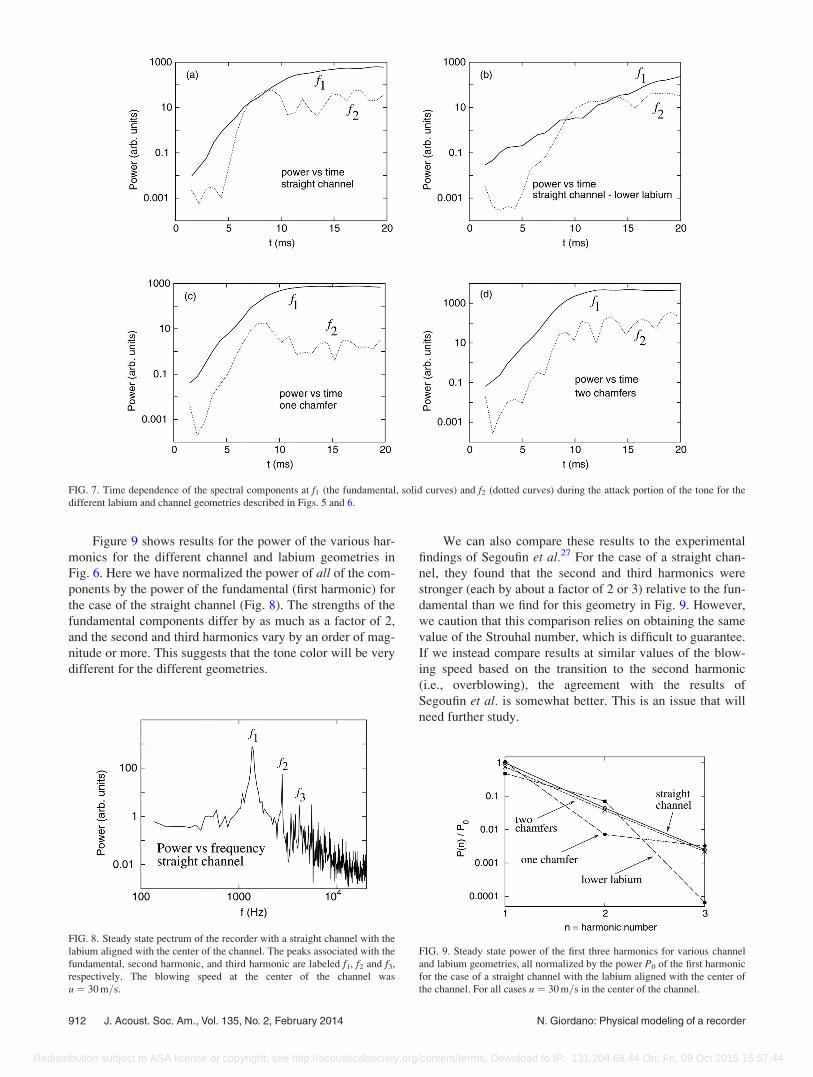
Figure 9 shows results for the power of the various har-

monics for the different channel and labium geometries in

Fig. 6. Here we have normalized the power of all of the com-

ponents by the power of the fundamental (first harmonic) for

the case of the straight channel (Fig. 8). The strengths of the

fundamental components differ by as much as a factor of 2,

and the second and third harmonics vary by an order of mag-

nitude or more. This suggests that the tone color will be very

different for the different geometries.

We can also compare these results to the experimental

findings of Segoufin et al.27 For the case of a straight chan-

nel, they found that the second and third harmonics were

stronger (each by about a factor of 2 or 3) relative to the fun-

damental than we find for this geometry in Fig. 9. However,

we caution that this comparison relies on obtaining the same

value of the Strouhal number, which is difficult to guarantee.

If we instead compare results at similar values of the blow-

ing speed based on the transition to the second harmonic

(i.e., overblowing), the agreement with the results of

Segoufin et al. is somewhat better. This is an issue that will

need further study.

FIG. 7. Time dependence of the spectral components at f1 (the fundamental, solid curves) and f2 (dotted curves) during the attack portion of the tone for the

different labium and channel geometries described in Figs. 5 and 6.

FIG. 8. Steady state pectrum of the recorder with a straight channel with the

labium aligned with the center of the channel. The peaks associated with the

fundamental, second harmonic, and third harmonic are labeled f1, f2 and f3,

respectively. The blowing speed at the center of the channel was

u ¼ 30 m=s.

FIG. 9. Steady state power of the first three harmonics for various channel

and labium geometries, all normalized by the power P0 of the first harmonic

for the case of a straight channel with the labium aligned with the center of

the channel. For all cases u ¼ 30 m=s in the center of the channel.



V. THE EFFECT OF EARS ON THE TONE OF AHYPOTHETICAL ORGAN PIPE

All of our discussion to this point has concerned channel

and labium geometries that might be found in a recorder. An

interesting geometry that is common in organ pipes (but not

recorders) involves the addition of “ears” to the sides of the

flue opening. These are flat plates placed on the sides of the

opening and extending well above the top of the channel.

Figures 10 and 11 show the behavior of the attack portion of

the tone when ears are added to a recorder with a straight

channel and labium aligned with the center of the channel.

The ears of this hypothetical organ pipe extended 5.0 mm

above the top edge of the labium (along the y direction) in

Fig. 1(a) and were 12.0 mm long along the x direction,

extending 4.0 mm to either side of the flue opening. This ear

geometry was not taken from any particular organ pipe (and

they may be a bit larger than commonly found in real

organs). Our goal here was simply to understand the kinds of

effects they can have on the behavior.

Here again we see at early times (5–10 ms) a strong

peak near the frequency of the second harmonic, with a fre-

quency f2 distinctly below 2� f1. Comparing with the result

for a straight channel without ears [Fig. 6(a)], we find that

the ears strengthen the power at f2 so that at early times this

component is stronger than the fundamental component. The

ears also affect the fundamental frequency of the steady state

tone, shifting it to a slightly lower frequency, as expected

because the presence of ears increases the effective length of

the resonator at the end near the labium. In our case, we find

a shift of about 20 Hz (approximately 1.5%). These results

confirm that the effect of ears is sufficiently large to be of

great use in tuning the instrument, both with regard to the

pitch and to the nature of the attack.

Not surprisingly, the ears also affect the dynamics of the

air jet. Figure 12 shows images of the jet at two separate

times on two vertical planes that pass through the channel

and flue opening. The top images show the air jet on the

plane that passes through the middle of the channel while the

bottom images show the air jet at the same times but on a

FIG. 10. Sound pressure as a function of time during the attack portion of

the tone for a flue pipe with ears.

FIG. 11. (Color online) Spectrum at early times for a flue pipe with ears

computed in the same way as the spectra in Fig. 6.

FIG. 12. Images of the air jet for a recorder with ears, all on an x� y plane [Fig. 1(a)] that cuts through the recorder. (a) and (b) For the plane that passes

through the center of the channel. (c) and (d) For a plane that passes just inside one of the side edges of the channel. Images (a) and (c) were recorded at the

same time, and images (b) and (d) were recorded approximately half a period later. The blowing speed was u ¼ 30 m=s.



plane that passes just inside a side edge of the channel and is

thus very close to an ear. One would expect the presence of

a nearby ear to somewhat dampen the motion of the jet due

to the nonslip condition on the velocity at the surface of the

ear, and that is precisely what is seen in Fig. 12. In the bot-

tom images (obtained near an ear), the jet loses speed much

sooner as it moves up and away from the channel, due to this

damping. This effect is also visible but not quite as great for

geometries without ears (as in Fig. 3) and will need to be

taken into account in any detailed comparisons between ex-

perimental and numerical results for the jet shape and

dynamics.

VI. EFFECTS AT HIGH BLOWING SPEEDS

All of the results shown in the preceding text were

obtained at blowing speeds for which the recorder oscillated

in its fundamental mode. As the blowing speed was

increased, the harmonics increased in strength and eventu-

ally the second harmonic became largest.

Maps of the air density at a blowing speed for which

oscillations at the second harmonic (with frequency f2) were

dominant are shown in Fig. 13. The image in (a) shows a

standing wave with nodes near both ends of the resonator

tube and at the center, giving a wavelength equal (apart from

end corrections) to the length of the pipe, as expected for an

oscillation at the second harmonic. The image in (b) was

recorded approximately half a period [a time 1=ð2f2Þ] later

and the image in (c) was obtained a half period after that.

Taken together the results in Fig. 13 show precisely the

behavior expected for this mode.

Figure 14 shows a series of images of the speed of the

air jet for the same conditions. These images span approxi-

mately one period of an oscillation at the fundamental fre-

quency f1. From these images, one can see the periodicity at

the frequencies of both the fundamental and the second har-

monic. For example, images (b) and (f), which differ in time

by 1=f2, both show the air jet extending upward above the la-

bium, but the detailed spatial variation of jet speed is dis-

tinctly different in the two cases. This can be explained by

FIG. 13. Images of the density for a blowing speed of 45 m/s. Here the spec-

trum was dominated by the component at the frequency of the second har-

monic f2 although the first harmonic was not completely negligible (see

following text). These images were obtained at times spaced by approxi-

mately half a period of the oscillation, 1=ð2f2Þ.

FIG. 14. Images of the air jet for a

blowing speed of 45 m/s for which the

oscillation at the second harmonic is

dominant. These images span approxi-

mately one period of the fundamental

frequency of oscillation.



an oscillation with two spectral components with frequencies

that differ by a factor of two.

Some parameters associated with the spectra for differ-

ent blowing speeds are shown in Figs. 15 and 16. There is a

clear transition to a mode dominated by the second harmonic

of the resonator tube. This transition occurs near u¼ 37 m/s,

as can be seen from Fig. 16. As u is increased through that

transition, the frequency of the second harmonic drops a

small but noticeable amount, and the frequency of the funda-

mental also decreases slightly (this decrease is barely visible

in Fig. 15). Above that blowing speed, the component at the

third harmonic becomes negligibly small. This transition has

been observed in many experiments (and by many recorder

players) and is often studied by observing how the frequency

varies as the blowing speed is gradually increased or

decreased. Such experiments generally show hysteresis; that

is, a range of blowing speeds for which the frequency can

assume two different values, depending on how the blowing

speed is varied. As we have performed our modeling, we are

not able to study this hysteresis; in our simulations, we have

always started each simulation with a blowing speed of zero,

which is then ramped quickly (in 5 ms) to a final value.

Comparisons of the results in Figs. 15 and 16 with

experiments must take account of this difference between

the experiments and our modeling.

Figure 17 shows the behavior of f1 on an expanded

scale. The results suggest that there are three different

regimes. (1) A region at low u, below about 20 m/s, where

the behavior is either dominated by or heavily influenced by

the edge tone. This was shown nicely by the results of Ref.

14 in two dimensions. In this regime, Miyamoto and co-

workers showed that the frequency is approximately propor-

tional to u as expected theoretically and thus falls rapidly as

u is decreased. (2) A region at high u where the behavior is

affected by the transition to the second harmonic. In Fig. 17

that region is above about u¼ 35 m/s. (3) An intermediate

region where the variation of f1 with u is much weaker. This

is presumably the musically useful range.

Bak29 reported a study of the variation of pitch with

blowing speed for a number of different notes with a number

of different recorders. He found behavior consistent with

f1 � kua; (8)

and his results are all consistent with a � 0:05. The straight

line in Fig. 17 shows a power law dependence and is consist-

ent with our results in region 3 defined in the preceding text.

The straight line drawn in Fig. 17 corresponds to a � 0:085,

and even allowing for generous uncertainties this is a consid-

erably higher exponent than the value found by Bak. The

reason for this difference is not clear, but it may be due to

the fact that our model recorder is much shorter than the

recorders studied by Bak. We speculate that this may make

the end corrections in our case more sensitive to u; this is an

issue that needs further study.

VII. SUMMARY AND OUTLOOK

We have used a direct numerical solution of the

Navier–Stokes equations to study the aeroacoustics of the re-

corder in three dimensions. We have shown how such simu-

lations can yield qualitative information concerning the

dynamics of the density and air jet, and quantitative results

for the sound spectrum and how it depends on blowing

speed. We have explored how the attack portion of the tone

depends on the detailed geometry of the channel and labium

FIG. 15. Frequencies of the three lowest spectral components during the

steady state portion of the tone as a function of blowing speed u in the center

of the channel. The labels indicate the fundamental frequency f1 and its har-

monics f2 and f3.

FIG. 16. Power of the three lowest harmonics during the steady state portion

of the tone as a function of blowing speed u in the center of the channel.

FIG. 17. Frequency of the oscillation frequency as a function of blowing

speed u. On this log-log plot a straight line indicates a power law variation

of f1 with u.



and found a significant inharmonic component at early

stages of the attack. We also find that the timbre of the

steady state tone depends strongly on this geometry. It will

be interesting to explore how this dependence on channel

and labium geometry might be used to produce recorders

with different tonal and playing properties.

One purpose of the present work was to demonstrate

that the computational methods used here give an accurate

description of the aeroacoustics of interest in a wind instru-

ment. We believe that our results do indeed confirm this

point and set the stage for applying these methods to study

other aspects of flue instruments and of other wind instru-

ments in general. Full musical tones that could be used in lis-

tening tests should be feasible soon.

ACKNOWLEDGMENT

I thank the Rosen Center for Advanced Computing at

Purdue University for access to the computational resources

essential for this work.

1N. Giordano, “Direct numerical simulation of a recorder,” J. Acoust. Soc.

Am. 133, 1113–1118 (2013).2P. A. Skordos, “Modeling of flue pipes: Subsonic flow, lattice Boltzmann

and parallel distributed distributed computers,” Ph.D. thesis, MIT,

Cambridge, MA, 1995.3P. A. Skordos and G. J. Sussman, “Comparison between subsonic flow

simulation and physical measurements of flue pipes,” in Proceedings ofthe International Symposium on Musical Acoustics, Dourdan, France

(1995), pp. 1–6.4H. K€uhnelt, “Simulating the mechanism of sound generation in flutes

using the lattice Boltzmann method,” in Proceedings of the StockholmMusic Acoustics Conference (SMAC 03), SMAC1–SMAC4 (2003).

5H. K€uhnelt, “Simulating the mechanism of sound generation in flutes and

flue pipes with the lattice-Boltzmann-method,” in Proceedings of theInternational Symposium on Musical Acoustics, Nara, Japan (2004), pp.

251–254.6H. K€uhnelt, “Vortex sound in recorder- and flute-like instruments:

Numerical simulation and analysis,” in Proceedings of the InternationalSymposium on Musical Acoustics, Barcelona, Spain (2007), pp. 1–8.

7A. R. da Silva and G. Scavone, “Coupling lattice Boltzmann models to

digital waveguides for wind instrument simulations,” in Proceedings ofthe International Symposium on Musical Acoustics, Barcelona, Spain

(2007), pp. 1–7.8A. R. D. Silva, H. K€uhnelt, and G. Scavone, “A brief survey of the lattice-

Boltzmann method,” in Proceedings of the International Congress onAcoustics, Madrid, Spain (2007), pp. 1–6.

9Y. Obikane and K. Kuwahara, “Direct simulation for acoustic near fields

using the compressible Navier–Stokes equation,” in Computational FluidDynamics 2008 (Springer, New York, 2009). pp. 85–91.

10Y. Obikane, “Direct simulation on a fipple flute using the compressible

Navier–Stokes equation,” World Acad. Sci. Eng. Technol. 4, 794–798

(2009).11Y. Obikane, “Computational aeroacoustics on a small flute using a direct

simulation,” in Computational Fluid Dynamics 2010, edited by A.

Kuzmin (Springer-Verlag, New York, 2010), pp. 435–441.12M. Miyamoto, Y. Ito, K. Takahashi, T. Takami, T. Kobayashi, A. Nishida,

and M. Aoyagi, “Applicability of compressible LES to reproduction of

sound vibration of an air-reed instrument,” in Proceedings of theInternational Symposium on Musical Acoustics, Sydney and Katoomba,

Australia (2010).13M. Miyamoto, Y. Ito, K. Takahashi, T. Takami, T. Kobayashi, A. Nishida,

and M. Aoyagi, “Numerical study on sound vibration of an air-reed instru-

ment with compressible LES,” arXiv:1005.3413v1.14M. Miyamoto, Y. Ito, T. Iwasaki, T. Akamura, K. Takahashi, T. Takami,

T. Kobayashi, A. Nishida, and M. Aoyagi, “Numerical study on acoustic

oscillations of 2d and 3d flue organ pipe like instruments with compressi-

ble LES,” Acta Acust. Acust. 99, 154–171 (2013).15K. Takahashi, T. Iwasaki, T. Akamura, Y. Nagao, K. Nakano, T.

Kobayashi, T. Takami, A. Nishida, and M. Aoyagi, “Effective techniques

and crucial problems of numerical study on flue instruments,” Proc. Meet.

Acoust. 19, 035021 (2013).16N. Giordano, “Direct numerical simulation of the recorder in two and three

dimensions,” Proc. Meet. Acoust. 19, 035062 (2013).17N. Giordano, “Numerical modeling of a recorder in three dimensions,” in

Proceedings of the Stockholm Music Acoustics Conference (SMAC 13),SMAC1–SMAC5 (2013).

18J. Martin, The Acoustics of the Recorder (Moeck, Berlin, 1993), 112 pp.19J. J. D. Anderson, Computational Fluid Dynamics (McGraw-Hill, New

York, 1995), 574 pp.20R. W. MacCormack, “The effect of viscosity in hypervelocity impact cra-

tering,” AAIA Paper 69–354, 1–7 (1969).21A. Jameson, W. Schmidt, and E. Turkel, “Numerical solution of the Euler

equations by finite volume methods using Runge Kutta time stepping

schemes,” AAIA Paper 81–1289, 1–14 (1981).22D. Botteldooren, “Acoustical finite-difference time-domain simulation in a

quasi-Cartesian grid,” J. Acoust. Soc. Am. 95, 2313–2319 (1994).23D. Botteldooren, “Finite-difference time-domain simulation of low-

frequency room acoustic problems,” J. Acoust. Soc. Am. 98, 3302–3308

(1995).24L. L. Beranek, “Acoustic impedance of commercial materials and the per-

formance of rectangular rooms with one treated surface,” J. Acoust. Soc.

Am. 12, 14–23 (1940).25B. Fabre, A. Hirschberg, and A. P. J. Wijnands, “Vortex shedding in

steady oscillation of a flue organ pipe,” Acta Acust. Acust. 82, 863–877

(1996).26G. K. Batchelor, “Computation of the energy spectrum in homogeneous

two-dimensional turbulence,” Phys. Fluids Suppl. 12, II-233–239 (1969).27C. S�egoufin, B. Fabre, M. P. Verge, A. Hirschberg, and A. P. J. Wijnands,

“Experimental study of the influence of the mouth geometry on sound pro-

duction in a recorder-like instrument: Windway length and chamfers,”

Acta Acust. Acust. 86, 649–661 (2000).28A. W. Nolle and T. L. Finch, “Starting transients of flue organ pipes in

relation to pressure rise time,” J. Acoust. Soc. Am. 91, 2190–2202 (1992).29N. Bak, “Pitch, temperature and blowing pressure in recorder playing.

study of treble recorders,” Acustica 22, 296–299 (1969).



simulation studies of a recorder in three dimensions

Documents