simulation project strategies - suraj @ lumssuraj.lums.edu.pk/~te/simandmod/opnet/09...

577-Sim

Simulation Project Strategies

Chapter 9

578-Sim

Modeling Concepts

579-Sim

Modeling Concepts IntroductionS

imu

lation

Pro

ject S

trategies

Sim.1 Introduction

OPNET is your “right-hand man” when it comes to decision making. It is hereto help you make decisions concerning many aspects of your IT systems and net-works. Most decisions involve an analysis of trade-offs for a range of solutions. OP-NET helps you make the right decisions by showing you what would be difficult orimpossible to achieve without simulation—the impact of each of the solutions youare considering.

The general objective of this chapter is to provide you with practical approachesto building models and running network simulations so that you can obtain mean-ingful results. The results provided by OPNET’s simulations are a function of themodels that you are working with and the data that you enter for parameters of themodels. To help you build models that achieve their purpose, this chapter informsyou about the following:

•

General concepts applied throughout OPNET’s standard model li-brary

. This is the library of models available to you as objects. You useobjects in a “plug-and-play” fashion; there is never any “programming”when you work in OPNET.

•

Important principles of simulation and modeling

. You will learn orreview basic concepts you should keep in mind throughout the model-ing process. Common techniques for simulation studies, such as base-lining and validation are discussed.

•

Specific Instructions for using particular components in the li-brary

. As in real networks, OPNET’s protocols and applications can bequite complex. Customization of these elements is achieved by settingparameters (that is, modifying the attributes of objects). In this chapteryou will find both general concepts and step-by-step instructions relat-ing to some of the major protocols and applications in the library.

•

Tips and techniques that will enhance your productivity

whenworking with many of the models in the library.

•

Methodologies for solving tough problems

such as simulating largenetworks efficiently, and analyzing and improving application re-sponse times.

580-Sim

Overview of the Standard Model Library Modeling Concepts

Sim.2 Overview of the Standard Model Library

OPNET provides an extensive library of models that you can use to build net-works. These models are called “standard models” because it is also possible for us-ers to develop their own models. Those models can then be shared with otherOPNET users if desired. Some users contribute models to the user community at nocharge. These are called “contributed” models, and are available in each softwarerelease. Other application-specific models are developed and sold by third partiesfor a fee. Of course, these models do not appear on your release CD.

In most cases, users work primarily with objects from the standard model li-brary. It is worthwhile to spend some time discovering what is available in this li-brary, how it is organized, and how to use the objects it provides.

Sim.2.1 Organization of the Model Library

The standard model library consists of the following types of objects:

• Devices

• Links

• LANs and clouds

• Utility objects

In actuality, the library also contains many models of networking protocols andalgorithms that allow your network models to simulate real network behavior.However, as a user of OPNET, you do not manipulate the internals of these proto-cols directly. Instead, you have access to the protocols’ functions via parameters,much as you do in working with real networks. Their parameters appear as at-tributes of the object types enumerated above and are easily configured via OP-NET’s GUI. One of the goals of this chapter is to explain the objects you haveavailable to you, and how to work with their attributes to represent your networksas desired within the tool.

Device Models

Devices comprise the majority of the objects in the standard model library. Theycorrespond to a wide class of network hardware, including the following:

• Routers

• Switches

• Hubs

• Workstations

581-Sim

Modeling Concepts Overview of the Standard Model LibraryS

imu

lation

Pro

ject S

trategies

• Servers

• Firewalls

• Printers

As you can see, devices essentially correspond to the “boxes”, that is, the “chas-sis-type” or rack-mounted systems in your network. They represent the hardwarethat performs the information transmission and processing in the network, rangingfrom simple repeaters like hubs, to content and computation servers, like mainframecomputers. Of course, these devices must not consist solely of hardware; most ofthem contain large amounts of software models, spanning appropriate layers of theprotocol and application stack. What’s inside a device depends on what its functionis. For example, a typical router model will contain hardware and software modelsof Ethernet, PPP, and perhaps other Layer 2 protocols. It will also contain and rout-ing protocols such as RIP, OSPF, IGRP, and BGP4.

The standard model library presents device models to you graphically. Typical-ly, you will select these objects from the object palette where they appear graphi-cally, though in some cases, you may choose their name from a menu of availablemodels. Once deployed into your network model, devices appear as icons. The stan-dard model library follows conventions (third party or supplemental models maynot) for the appearance of each type of device, as illustrated below:

Vendor versus Generic Device Models

Device models are also categorized into two classes: vendor device models andgeneric device models. Vendor models represent devices manufactured by a partic-ular company, such as Cisco Systems or 3Com. The developers of the standardmodel library use data published by these manufacturers to characterize the devicesas well as they can. You can also create vendor device models using the “DeviceCreator” operation, provided you have obtained values for required parameters ofthe device.

LAN Switch Router

WorkstationServerHubPrinter

Graphical Conventions for Network Objects

582-Sim


Generic models provide behavior that is appropriate for devices of their class.However, they are not configured to model any particular manufacturer’s devices.Instead these devices provide attributes (that is, parameters), allowing you to con-figure each one you deploy differently if you choose. For example, the generic rout-er below offers the attribute “forwarding rate”, which specifies the throughput ofthe router in packets per second. Each instance of the router that is deployed can beassigned its own forwarding rate. In contrast, a vendor device model of a routerwould already be aware of its own forwarding rate, as you would expect since thedevice type is already known. A vendor model would therefore not provide the “for-warding rate” attribute.

In later sections of this chapter, we will discuss practical aspects of workingwith the devices in the model library.

Link Models

To form a network of devices, you will need to use links and these links willrequire specific characteristics. In OPNET, links represent the physical media andproperties, such as line rate in bits per second, delay, and likelihood of data corrup-tion. Link models also generally represent a choice of layer 2 technology, allowingOPNET to verify compatibility of two or more attached devices, and the link thatconnects them. One of the most important characteristics of a link model from a net-work performance perspective, is the speed of transmission, in bits per second. Thischaracteristic is usually implicit in the choice of link model (for example, a10BaseT link automatically provides for a 10 Mb/sec. transmission rate).

Links are represented as line segments or a series of line segments with arrow-heads in the OPNET GUI. When selecting links from OPNET’s object palette, youwill see objects similar to those shown below:

Generic Model vs. Vendor Model

vendor model

generic model

(shows vendor logo)

Link Model Graphical Convention

583-Sim


imu

lation

Pro

ject S

trategies

LAN and Cloud Models

OPNET lets you model the “end systems” of your network in explicit detail,representing each device if necessary. However, in many simulation studies, youwill prefer to abstract local area network infrastructure into a single object, called aLAN object. The LAN object models many users on the same LAN, and allows fora server within the LAN as well. However, it does so within a single object, thusdramatically reducing the amount of configuration work you need to perform to rep-resent your internetwork of LANs. In addition, because fewer objects are present inyour network, LAN objects help reduce the amount of memory needed to performsimulation. LAN objects are provided for a variety of local area network technolo-gies, as shown below:

Using LAN objects you can quickly generate large amounts of users for yournetwork. Specifically, each LAN object allows you to specify the number of userspresent within it. You can then assign application traffic to a subset, or all of the us-ers of the LAN. Thus, scaling the traffic generated by a LAN (to model more users,for example), is a simple matter of increasing the specified number of users. LANscan then be interconnected via switches and routers to carry traffic to and from de-vices and LANs in other parts of the network.

In a manner similar to the use of LANs, it is sometimes appropriate to abstractparts of the wide area network infrastructure. Cloud models are special objects inthe model library used to represent such infrastructure. They provide high-levelcharacteristics used to simulate the behavior of that portion of the network. TheATM, Frame Relay, and IP model suites all include cloud models.

LAN Objects Abstract Local Area Infrastructure

Cloud Objects Abstract WAN Infrastructure

584-Sim


Cloud models can have numerous applications. For example, your backbonenetwork may depend on services delivered by an Internet Service Provider (ISP),which in turn may be connected to a carrier network. Since you do not know thedetails of the backbone, a cloud node gives you a simpler model without losing anydetail.

You may also find cloud models useful if you are more interested in modelingLAN infrastructures than network infrastructures. If your primary focus is on mod-eling details on LAN traffic flows, you may not want to model the backbone net-work in minute detail. Representing the backbone with a cloud should suffice.

You can simulate a backbone network using two cloud-model attributes:

•

Packet (or Cell) Latency.

This specifies the one-way delay that eachpacket experiences while traversing the network. You can run a simpletest on your network to determine this setting. First, configure yourping traffic (using an option like IP’s “record route”) to report the num-ber of hops that a packet traverses. Then measure the response time andnumber of hops for a typical ping packet sent across the network. (Keepin mind that this response time includes transmission delays at eachhop.) Once you have these two values, you can use the following equa-tion to compute the actual network latency:

Latency = (Ping Response Time – (Hop Count * (Ping Packet Size/Data Rate)))/2

Use the resulting value for the latency parameter. You can also specifyany built-in or custom distribution to model variability in the delay.

•

Packet (or Cell) Discard Ratio.

This specifies the ratio of packetsdropped to packets submitted to the network backbone. You can set thisvalue based on your network service provider’s statistics or its traffic-contract guarantees.

Utility Objects

Objects that don’t correspond to actual physical infrastructure are also some-times useful in constructing network models. In general, these perform a logicalfunction in the network, such as configuration of network resources on a global lev-el (for example, provisioning of permanent virtual circuits, or PVCs). Another typ-ical role for a utility object is to enable a simulation-specific function, such asreporting on use of memory resources. Finally, utility objects can be used to scriptspecial events in the simulation, such as the failure of a particular network elementat a given time. In all of these cases, utility objects are selected from the palette anddeployed into the network model, and in general their location does not matter.They have attributes that control their function in the simulation.

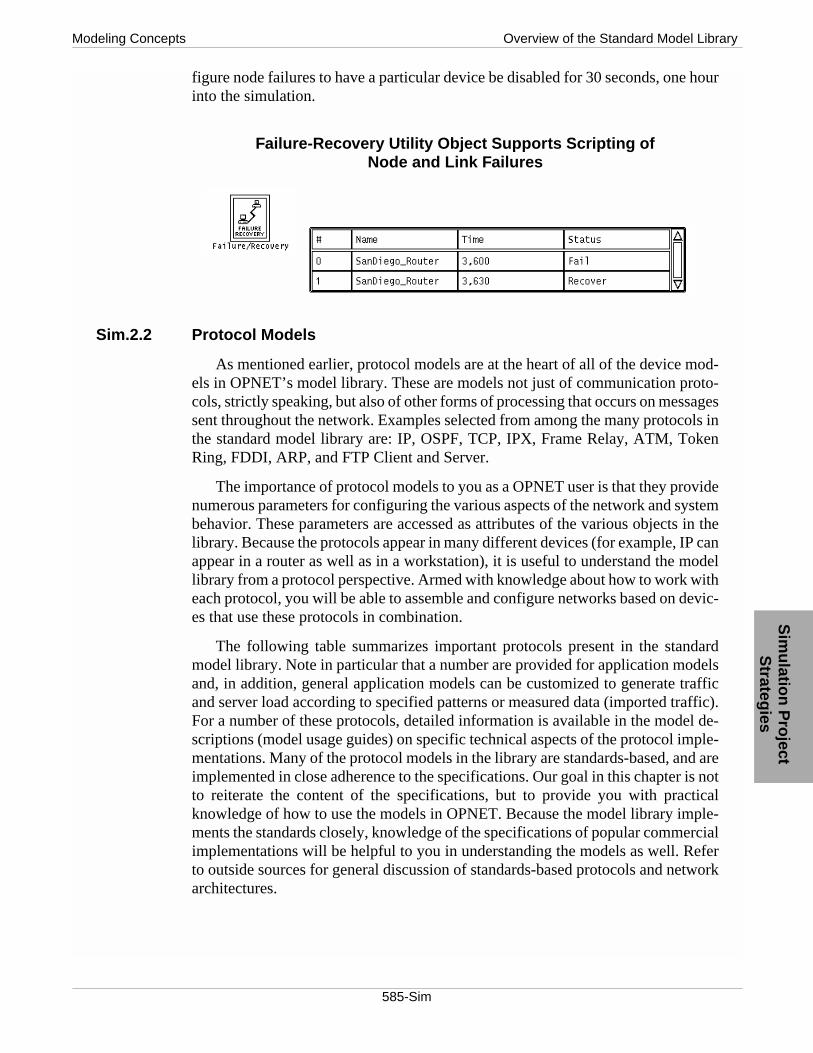
The “Failure-Recovery” utility object is one that is commonly used to introducenode or link failures at specific times. You can cause the same nodes/links to thenbecome operational (recover) at later times. The example below shows hot to con-

585-Sim


imu

lation

Pro

ject S

trategies

figure node failures to have a particular device be disabled for 30 seconds, one hourinto the simulation.

Sim.2.2 Protocol Models

As mentioned earlier, protocol models are at the heart of all of the device mod-els in OPNET’s model library. These are models not just of communication proto-cols, strictly speaking, but also of other forms of processing that occurs on messagessent throughout the network. Examples selected from among the many protocols inthe standard model library are: IP, OSPF, TCP, IPX, Frame Relay, ATM, TokenRing, FDDI, ARP, and FTP Client and Server.

The importance of protocol models to you as a OPNET user is that they providenumerous parameters for configuring the various aspects of the network and systembehavior. These parameters are accessed as attributes of the various objects in thelibrary. Because the protocols appear in many different devices (for example, IP canappear in a router as well as in a workstation), it is useful to understand the modellibrary from a protocol perspective. Armed with knowledge about how to work witheach protocol, you will be able to assemble and configure networks based on devic-es that use these protocols in combination.

The following table summarizes important protocols present in the standardmodel library. Note in particular that a number are provided for application modelsand, in addition, general application models can be customized to generate trafficand server load according to specified patterns or measured data (imported traffic).For a number of these protocols, detailed information is available in the model de-scriptions (model usage guides) on specific technical aspects of the protocol imple-mentations. Many of the protocol models in the library are standards-based, and areimplemented in close adherence to the specifications. Our goal in this chapter is notto reiterate the content of the specifications, but to provide you with practicalknowledge of how to use the models in OPNET. Because the model library imple-ments the standards closely, knowledge of the specifications of popular commercialimplementations will be helpful to you in understanding the models as well. Referto outside sources for general discussion of standards-based protocols and networkarchitectures.

Failure-Recovery Utility Object Supports Scripting of Node and Link Failures

586-Sim


Standard Model Library Protocols

Layer 1, 2 and Support Layer 3 and Support Layer 4 Application

ATM ATM TCP FTP

Ethernet 10, 100, 1000 IPX UDP E-Mail

ARP Frame Relay NCP HTTP

Frame Relay IP Voice

FDDI OSPF Video

Token Ring 4, 16 RIP Database

PPP BGP4 Printing

SLIP IGRP Remote Login

Spanning Tree X.25 General Background Traffic

ATM LANE Customized 2 tier

X.25 (LAPB) Customized Multi-tier

587-Sim

Modeling Concepts Essential Approaches to Modeling and SimulationS

imu

lation

Pro

ject S

trategies

Sim.3 Essential Approaches to Modeling and Simulation

Many people would have you believe that Modeling is a task of extreme diffi-culty that requires years of training to perform successfully. This is not the case,particularly given the availability of modern modeling tools like OPNET. One ofthe keys to success that OPNET brings you is its model library, which incorporatesvery significant modeling capabilities “packaged” into easy to use objects. Usingthese packaged components not only means that less modeling expertise is required,but also that modeling efforts are dramatically shortened because you can focus ondomain-specific issues (that is, application, system, and network issues), rather thanon detailed implementation of models.

Even within a tool like OPNET, however, you will still need to make certainchoices as you construct models and run simulations. This section discusses generalprinciples of modeling and simulations that will help you consider your alterna-tives. Subsequent sections explain how to use particular components of the modellibrary as well as methodologies for solving particular problems with OPNET.

Sim.3.1 Equivalence: The Core Concept of Modeling

The most important thing to remember in carrying out your projects is that mod-eling is fundamentally about “equivalence”. In other words, your objective is tobuild a model that is equivalent to a real system, existing or proposed. However,“equivalent” is a subjective term which must be defined more precisely. Clearly,equivalence means that your model behaves in some sense like the real system.Nevertheless, for practical reasons, models are usually limited to representing onlycertain aspects of the system of interest. Therefore, it is up to you to define equiva-lence for your modeling project, with the following objectives in mind:

•

The model must answer the questions of interest

. You want to usethe model to help you study a particular set of issues. You need to de-fine those issues clearly before you start your modeling effort. Know-ing which questions are important will allow you to exercise goodjudgement in including or omitting certain features in your model. Theanswers you obtain from your model and their utility are the ultimatebenchmark of your modeling effort’s success.

•

The model should have the desired level of accuracy

. Your model’saccuracy can probably not be perfect, but you need to have a notion ofwhether you are making simplifications in your model to the pointwhere the answers it provides will no longer be useful. Depending onwhat types of actions you will take as a result of your model’s predic-tions, you should determine how conservative you want to be with re-spect to simplifications.

•

The model should support validation

. As you design your model, youshould have a plan for building confidence in the results it produces.

588-Sim

Essential Approaches to Modeling and Simulation Modeling Concepts

•

Your model should accommodate the necessary range of operatingconditions.

Usually, the system of interest, and therefore the model, issubjected to a range of different stimuli. For a network model, this maymean increased application traffic, or new application patterns, for ex-ample. If you know the range of conditions you want to study, considerhow to ensure your model will maintain its validity throughout thatrange.

So equivalence is really a function of what you want the model to help you ac-complish. As you make each modeling choice, such as which component to usefrom the model library, you need to ask yourself if this choice could disturb theequivalence which you have achieved so far, or if it enhances it. Even if it does insome sense “lessen” the equivalence between your model and your system, does itachieve another benefit for you that is worthwhile, such as reduced simulation runtimes? And then finally, can you measure the relative loss or gain of equivalence tohelp you determine if it is acceptable?

The important point is that good modeling practitioners do not necessarily haveprecise answers to all of these questions, but they keep these issues in the forefrontof their minds as they make modeling choices. This is something you should do aswell as you consider various approaches to representing your system as a model.

Sim.3.2 What Should You Include in Your Model?

Many of the important choices you make in developing a model have to do withselecting aspects of the real system to include or not to include. One approach is toinclude everything that you are aware of, to ensure that you are not neglecting anyimportant mechanism. The problem with this approach is it can be too time-con-suming in terms of building the model and also that it can produce a model that istoo computationally expensive. In other words, simulations may take longer to runthan desirable, or than is necessary to get good results.

Choosing which behaviors to represent in a model is one of the most difficulttasks a modeler faces. This makes sense since the modeling effort is supposed toteach us which parts of the system are responsible for the system behaving or per-forming a particular way. Thus, it is hard to know in advance which aspects of thesystem are significant. So, you are required to make a judgement. Your decisionswill later have to be backed up through validation. Your initial model should bebased on a “list of suspects” if you are investigating a problem in your network, orif you anticipate possible problems with a future network or modified network. Inother words, you should make an educated hypothesis about what will matter to an-swer your questions. Then, you can change your hypothesis and build several othermodels that emphasize different aspects of the system. This will help you learn whatis significant and what is not with respect to your particular objectives.

If you are working in a component-oriented environment like OPNET, you havea library of models that are packaged for ease-of-use. This helps to clarify yourchoices. Your basic choices relate to the following:

589-Sim


imu

lation

Pro

ject S

trategies

• which objects should you use from the library?

• which protocols should you enable?

• how should you assign the attributes of objects?

• how should you model traffic in the network? Should you use explicitapplication traffic, packet trace-generated traffic, background traffic, ora combination? These traffic modeling terms are explained in more de-tail in later sections.

Since your modeling decisions as a OPNET user are guided by the model li-brary, the majority of this chapter focuses on assisting you in understanding itsmodels and how to work with them.

Sim.3.3 Model Validation

Regardless of the approach you choose in developing your models, validationis a key step before using results to draw conclusions. In fact, validation is a stepthat is generally performed repeatedly during the course of model development, asyou continue to add enhancements. By verifying fundamental behaviors of yourmodel at each step, you can maintain a high degree of confidence, and easily iden-tify which particular changes are responsible for new, unexplained behavior. Incontrast, if you make many simultaneous changes before examining the model’s be-havior, you will then be unable to determine which changes are responsible for yourobservations, and to what extent each change has contributed. In short, after youbuild your first basic model of your system, you should progress incrementally, per-forming validation at each step.

Even though validation sounds like a formal term reminiscent of a mathematicalproof, or formal verification, it need not be handled in that manner. Rather, valida-tion is the process of maintaining confidence in your model’s equivalence to the realsystem and in its ability to generate useful results. Therefore, you are again respon-sible for determining what is necessary to achieve this confidence. Typically, youwill make use of a combination of several techniques, outlined below:

•

Common Sense and Intuition

. Simplistic as it may seem, this is yourmost important tool in model validation. Even if you cannot tell if ananswer is correct, or what its degree of accuracy is, you should have anopinion on whether an answer is “in the right ball park”, or significantlydifferent than what you would consider plausible. If it is not, the modelcould still be correct, but it’s time to investigate further.

Your common sense and intuition may come from your experience withthe real system, or with the technologies at hand. You may also be re-lying on crude mathematical calculations you have performed, whichserve as a “boundary analysis”. The boundary analysis is a simple cal-culation that you expect to definitely be lower or higher, as the case

590-Sim


may be, than the answer your model will produce. In other words, if youknow that your model accounts for certain effects that your calculationdoes not, try to determine if those effects would modify the result in onedirection or another.

For example, will accounting for packet fragmentation and overheadincrease application response times or decrease them? You would prob-ably answer increase them, so if your simulation model does performfragmentation, and your simple calculation does not, you might expectthe simulation model to predict higher response times.

•

Measurement

. This is the most common approach to validation andthe one most people think of first. Some people refer to it as “baselin-ing” against the real system. Of course, it can only be done if the realsystem, or some portion of it, is actually accessible. Measurement toolscan consist of network analyzers, such as Network Associates’ Sniffer,or those manufactured by Wandel & Goltermann, Hewlett Packard, orone of many other vendors; or they can be as simple a stopwatch formeasuring the interval required to complete an activity. Some net-works, applications, or protocols are also instrumented to report on cer-tain aspects of their performance.

Here again, you should have a notion of what the differences are be-tween your model and your real system. When the results differ, as theytypically do initially, you will want to make a judgement about whetherthe differences can be attributed to simplifications in your model. Isyour model operating under all of the same conditions as the real sys-tem?

As an important side-note, many people think of measurement purelyas a validation tool. In fact, measurement can be a powerful modelingtool as well. Later, we will discuss how to use measurements as a com-ponent within your model.

•

Alternative Models.

By building another model using a different ap-proach, you can gain insight into how both models behave and whichone will do the best job for you. In other words, which is providing“more valid” results for the questions you want to answer under the op-erating conditions that matter. The alternative model may not be yourown. It may have already been provided or had its results published byanother party. It may also be a model of a completely different nature,such as a mathematical or “analytical” model. Essentially, what you aredoing here is very similar to the technique of performing measure-ments, but in this case, your “measurements” are taken in another mod-el of the system instead of the system itself.

•

The Control Experiment

. This is a technique familiar from high-school science classes. Build a test case in which you know what the re-sults should be with a high degree of confidence. Typically, this is done

591-Sim


imu

lation

Pro

ject S

trategies

by using extreme operating conditions to isolate particular behaviors ofthe model. For example, what is the application response time if theserver is infinitely fast and transactions are very small so that requestsand responses can easily fit into one packet? Under these conditions,you can generally do a good job of making a simple manual estimateand compare against your simulation. A good comparison will buildyour confidence for moving to the next step: changing one aspect of thetest case. In this example, that might be changing the transaction size.The fundamental concept of the control experiment is to remove mostbehaviors that are difficult to explain and to use common sense to per-form validation in their absence. Then use incremental analysis, de-scribed below, to gradually re-introduce some of the other complexmechanisms in the system.

•

Incremental Analysis

. Making individual changes rather than manychanges at once has already been emphasized as a sound strategy. As avalidation technique, incremental changes and analysis of their impacthelps you understand if each change makes sense. In the final phases ofyour project, you will use this information to explain what were the sig-nificant factors in determining performance of your system. This willalso allow you to detect when certain mechanisms act in combinationto produce interesting behaviors. For example, a slow link may not bea problem for your system’s performance, nor may a low but non-zerorate of frame loss; but the combination of the two could cause your end-to-end response times to increase dramatically. In summary, the pur-pose of incremental analysis is to experiment with the model’s param-eters to gain confidence with the behavior of individual features.

Validation is a rewarding process as long as you are receiving confirmation thatyour model is providing “equivalence” with the real system, as you are expecting.However, this will not always happen, so you must have an approach to followwhen validation is negative. The following are some typical approaches you cantake in such a situation:

•

Return to the previous validated state

. If you have performed a vali-dation of the model at a previous stage, save your current model and re-turn to its previous form (this highlights the value of saving eachimportant version of your model, particularly at each validation). En-sure first that you can recreate the results you had before. Then individ-ually reintroduce changes you have made in order to validate them oneat a time. This will allow you to more easily determine which changehas caused your model’s validity to deteriorate.

•

Break the model down into parts that are easier to validate

. If youhave not already done so, validate simpler versions of this model. Re-move components that you consider non-essential to reach a pointwhere you feel the results make sense. With fewer objects in the sys-tem, you will also have fewer parameters to configure and less room for

592-Sim


error. Then, build back up again to a larger model, validating each stepalong the way.

•

Question all of your assumptions

. It is at this time that you will needto remember all of the important assumptions you have made. Assump-tions are either made about how the system really works, or about theminimal impact of a particular simplification. In a component-orientedmodeling environment like OPNET, your assumptions may be reflect-ed in which model library objects to use and how to set their parame-ters. You may also have made some assumptions about backgroundtraffic or imported packet traces. All of these “inputs” to the modelshould be re-examined, particularly those that you feel may impact thevalidation significantly.

•

Validate the validation

. It is possible that instead of your model beingflawed in some way, it is the experiment itself that is flawed. A mea-surement may have been taken incorrectly, or misinterpreted. If you arecomparing against another model or mathematical calculation, thatmodel or calculation may be in error.

Exact Results and Useful Results

While highly accurate results are generally desirable, it is important to empha-size that validation does not always mean an exact matching of results between yoursimulation and your measurements, or whichever other form of comparison youchoose to use. Discrepancies are to be expected and can be accepted, provided thatyou feel that you understand them and are in control of them. In other words, youshould be able to account for differences and understand their importance relativeto the questions you are trying to answer.

One common approach where exact results are not emphasized is “sensitivityanalysis”. Here the objective is to vary one of the “inputs” of the model (the averagesize of a response returned by an application server, for example) and determine itseffect on a model “output” (for example, the application response time). In such acase, you might be more concerned with the relationship between these two quan-tities, rather than whether they are exactly correct. In other words, is the responsesize a dominant factor in determining response time, or are other factors more im-portant? If, for example, you determine that the application’s response time variesvery little over the possible range of response sizes, you can focus your efforts oninvestigating other parts of the system.

Sim.3.4 Putting it All Together: the Modeling Process

You have been given a number of recommendations and techniques in this sec-tion. These techniques are generally incorporated as steps in an overall modelingprocess. The process is described below as a general map you can follow in yourmodeling and simulation projects. As always, you should feel free to adapt it as nec-essary if it makes sense for the objectives that you have set for yourself.

593-Sim


imu

lation

Pro

ject S

trategies

1) Develop a list of questions you want the model to answer.

2) Create a preliminary model that answers at least some of the questionsin 1. To do this, represent those aspects of the system that you feel havethe most impact on the questions of interest.

3) Validate the model to gain confidence in its “equivalence”. For eachdiscrepancy you find through your validation, decide if it is significant.Determine the sources of the discrepancies, if any. Correct them, andrepeat this step until satisfied that you have achieved an equivalencewith your real system. If you cannot achieve it with this model, youneed to go back to step 2 and choose a different approach.

4) Consider enhancements to your model to help you answer further ques-tions effectively. Do these changes disturb “equivalence” or enhance it?Experiment with the changes and validate them to understand them.This amounts to returning to steps 2 and 3.

5) When you are satisfied with your model, use it to analyze the set of cas-es or operating conditions you wish to study for your system. For a sim-ulation approach, like OPNET’s, this involves running simulations.Carefully examine the results of each simulation to ensure you under-stand them. Investigate any results that do not make sense to you.

6) When you are satisfied with the model’s performance, publish your re-sults, and document your modeling choices. This will support the ap-propriate use of the results, and the continued use of your model forfuture projects.

Sim.3.5 Simulation Issues

Running simulations is typically thought of as the next-to-last step in the simu-lation and modeling process, the last step being results analysis. However, in fact,simulation is typically performed many times within the modeling process, as de-scribed above. Individual simulations are used to validate and experiment. Finally,you will typically run a series of simulations to explore different issues and alterna-tives with your model. As you begin to run simulations you will be confronted witha few important issues concerning the configuration of your simulation runs. Thissection helps you understand these issues.

Sim.3.6 Simulation Duration and Number of Simulations to Run

One of the most common questions concerns selecting a duration for the simu-lation. “Duration” refers to the amount of time simulated, not to the amount of“wall-clock” time that it takes to complete the simulation. We generally refer to“wall-clock” time as “real-time”, and time modeled in the simulation, as “simula-tion time”. Determining the duration of a simulation is typically driven by one oftwo factors: how much activity to simulate to obtain valid results; or simply, the

594-Sim


time-span of activity that is required. The former requires some explanation, whilethe latter is obvious. Note however, that you should always ensure that sufficienttime has elapsed to allow representative activity to have occurred in your simulatedmodel, even if this means simulating a longer period than you are required to byyour project’s specification.

Randomness

Activities that have to be simulated are generally known to occur at a certain fre-quency or average rate. For example, if you are simulating users submitting trans-actions at a rate of 1 per minute and you want to obtain data on at least 30transactions for each user, then it is a simple matter to choose a minimum simula-tion duration of 30 minutes.

It is important to realize that most simulations involve an element of random-ness. It is possible to configure the traffic sources in the simulation to generate ap-plication requests or other forms of traffic in a perfectly regular pattern. However,this is typically not the case: instead, many parameters are configured with proba-bility functions that characterize the likelihood that a particular outcome would oc-cur. These probability functions are often referred to as PDFs, which stands for“probability density functions”.

For example, the time required for a server to generate a response to a client,given a request varies each time that it is measured. Given enough measurements atthe same time of day, on a typical day, we can construct a PDF for “Server ResponseGeneration Time”. OPNET in fact provides you a tool to do this using the “ImportPacket Trace” feature, which will be described later. This PDF can then be used totell OPNET server objects how to model response generation timing. Given that re-sponse generation time is slightly different, and that in addition, other parameters,such as response size and request size might also be variable, it is clear that overalltransaction response time, which is a function of all of these, will also be subject tofluctuation. This is identical to the situation we experience in real systems: eachmeasurement we obtain is different.

Since the statistic we are trying to analyze may be subject to fluctuation, we can-not completely trust the results of a single simulated activity, such as a transactionin the example above. Certainly, a single measurement tells us something, namelythat such a value is possible. This can be useful information in the sense that oneparticular measurement might be higher than what we consider acceptable and thattherefore the proposed design must be revisited. However, in general, we want toobtain a more complete picture by looking at a collection of “samples” for the quan-tity of interest. So, we would collect many transaction response times, either by run-ning a series of simulations, or simply by letting the simulation run longer so thatan application could “regenerate” another transaction at a later time.

Developing Confidence in Simulation Results

How many total samples are needed is a difficult question to answer. One of thereasons it is difficult is that this depends on the variability of the quantity of interest.

595-Sim


imu

lation

Pro

ject S

trategies

Intuitively, this makes sense, because if you obtain ten samples between 26 and 28with an average of 26.5, you have a strong sense that this is the range you can expectfor additional simulations, if you were to run them. Thus, you can be confident inpredicting the range and average, with just ten samples. However, if the same tensamples varied between 20 and 40 with values widely scattered between these twobounds, you would feel uneasy about not obtaining further information.

Confidence can be established for a set of gathered samples by extracting arange from the samples and giving a likelihood that the “real average” lies some-where in that range. By “real average” we mean the value we would obtain if wemeasured vast numbers of samples in the real system and computed their average.So, for our example, we might make a statement such as: “From simulations, wehave 95% confidence that the actual average response time is between 26 and 28seconds”. Again, this way of characterizing confidence makes intuitive sense be-cause we cannot ever be certain that the samples we obtained from simulation wereactually representative: they could all be exceptional values (so-called “fluke val-ues”); however, the chance that this would be the case diminishes quickly as wegather more samples. Thus, gathering more samples enhances our confidence, butnever provides a 100% guarantee. To increase our certainty, we can increase therange we are seeking for the average value, or we can obtain more samples.

While you can rely on your intuition to tell you if you have obtained enoughsamples, or some rules of thumb (many practitioners recommend the number 30 asa good number of samples), there are mathematical methods for determining confi-dence. OPNET helps you apply these methods by supporting the calculation of con-fidence intervals. These can be obtained in one of two ways:

• The “Statistic Info” operation provided for each graph allows you to seeconfidence intervals for 80%, 90%, 95%, 98%, and 99% confidencelevels for the collection of points presented in the graph. See the impor-tant caveat below, however.

• The “Show Confidence Intervals” operation graphically displays confi-dence intervals, but assumes your data was collected using the “scalarstatistic” collection approach, based on running many simulations. Itgenerally does not apply to graphs that have “time” as their horizontalaxis label. Scalar statistic collection is an advanced topic beyond thescope of this chapter.

When using confidence intervals, there is an important fact to be aware of con-cerning the relationship between the samples. These samples must be “indepen-dent”, which informally-speaking means no pair of samples must influence oneanother’s values or be linked indirectly to another condition that influences both oftheir values. In other words, the fact that the first sample was obtained should notinfluence the likelihood that the second sample would have been obtained. Such“dependencies” can occur in systems where state plays an important role. The fol-lowing examples, still based on application response time, will help you understandwhen you can consider your samples to be independent:

596-Sim


• A single client is connected through a network to a single server and re-quests are submitted one at a time via the network to the server. The ap-plication response time is measured each time a response is returned tothe client. Successive response times are measured for 25 transactions.

These samples are independent

because they have no influence overeach other. As each transaction completes, the system returns essential-ly to the same state it was in prior to the transaction being initiated. Youshould get a similar collection of results running individual simulationswith different random seed values and obtaining one sample per simu-lation.

• Many clients are connected via a network to one or more servers andsubmit requests to those servers. As in the previous example, a client’scurrent transaction must complete before it can submit another one. Re-sponse times for successive transactions are measured at a particularclient.

These samples are independent

even though there is concur-rent activity in the network, because the successive experiments still donot influence each other (or at least probably not significantly if theyare sufficiently spaced out in time). The activities of other clients canbe aggregated together and viewed as forming the statistical nature ofthe delay on the server. The fact that a first transaction was submittedby the client of interest does not significantly affect the response timefor the second transaction it submits.

• The configuration is the same as in the prior example; however, we arenow obtaining our samples from all clients. We may obtain hundreds orthousands of samples. So, the only difference is the fact that we are in-cluding more measurements from many locations. In this case,

thesamples are not independent

because consecutive samples are report-ed by different clients that have influenced each others’ behavior. Spe-cifically, if client A and B submit transactions at approximately thesame time and finish at approximately the same time, both will recorda result that is different than if they had submitted transactions separate-ly. This is true because of contention for processor resources, which ismodeled on the server. Thus, you cannot believe the confidence inter-vals provided by the “Statistic Info.” operation.

Finally, if you wish to use confidence interval measurements with the statisticsprovided by OPNET, read the following section on statistic collection for importantinformation on how to configure statistics of interest prior to simulation.

Collecting Statistics

Before running a simulation, you will generally specify which statistics youwish to collect. OPNET does not automatically collect all statistics in the system be-cause there are so many available that you may not have enough disk space to storethem. Specifying statistics is a straightforward task which is performed through theGUI, and this is not a time-consuming task in general.

597-Sim


imu

lation

Pro

ject S

trategies

There is one important subtlety associated with statistic collection, however.This has to do with how the reported statistics are processed by the simulator priorto being stored in the simulation results file(s). By default, nearly all statistics aregathered in what is called a “bucket mode”. “Bucket” refers to the fact that the sta-tistic’s values are grouped and processed to reduce the number of samples reportedin the statistic over the course of the simulation. This greatly reduces the amount ofdisk space required per statistic, which typically allows you to collect as many dif-ferent statistics as you desire.

You can think of the statistic as having an original set of values that are drivenby appropriate events in the simulation. The simulator then groups consecutivesamples that occur within a time interval, processes them together, and presentsthem as a single value. The time interval is the “bucket”, and the width of that buck-et (measured in seconds) can be controlled by the user. The simplest way to controlthis parameter is to change it for all statistics by setting the “Values per Statistic”parameter of the “Configure Simulation” dialog box before running a simulation.This implicitly determines the amount of time spanned by each bucket because itdivides the simulation duration (also specified in the same dialog box) into a fixednumber of intervals.

Continuing with the example of application response time measurement, groupsof values would correspond to not one, but many individual transactions completing(that is, returning completely to the client). Specifically, the response times for allthe transactions that occurred within buckets of, say 10 seconds, would be averagedtogether to plot just one value in the statistic’s graph. Similarly, utilizations for linksor PVCs are reported as the average utilization within a fixed-size bucket, not as in-stantaneous values. In general, bucket-oriented presentation of statistics is familiarand meaningful to most users, as this is the way information is often presented bynetwork monitoring or reporting tools. However, there are cases in which you willwant alternative ways of collecting and presenting data, as described in the remain-der of this section.

In addition to controlling bucket width for all statistics together, you can alsocontrol the bucket width and other aspects of statistic collection for each statistic,individually. You can do this by right-clicking on the statistic of interest in the“Choose Results” dialog box and selecting the “Change Collection Mode” opera-tion. The default configuration of the statistic appears as “Total of <default> Val-ues”. This means that the setting provided in the “Values per Statistic” parameter isto be used. You can choose a different number of samples, or you can use the “ad-vanced” mode of this dialog box to choose other collection modes (also termed cap-ture modes) in order to not use bucket-oriented collection at all.

Of particular interest is the “All Values” mode. This mode is important becauseit allows you to remove the effect of averaging or other processing performed in thebucket-oriented collection modes. Thus, you can observe measurements for indi-vidual transactions, for example, instead of seeing the averaged results of manytransactions that occurred within a bucket. This helps you gain a better understand-ing of what is actually happening within your simulation when you need to. It is par-ticularly recommended to use this mode for some statistics during validation

598-Sim


because you will gain more insight into the behavior of the model. Finally, usingthe “All Values” mode is essential if you wish to apply the approach describedabove for measuring confidence and determining if you have simulated a sufficientamount of the system’s activity.

Sometimes, what you will see using the “All Values” mode will surprise you.Consider a utilization statistic, for example. Utilization consists fundamentally ofan averaging of an on-off type of process. In other words, a link is either not in useor in use to transfer data at a given moment. To provide more insight into how thelink is being used over periods of time, OPNET performs averaging over buckets.But when you look at the low-level information using “All Values”, you will see astream of ones and zeroes. Furthermore, you will probably record many morepoints, so you should use the “All Values” collection mode cautiously, applying itonly to a small number of statistics at a time. As a second example, consider athroughput statistic, measured in bytes per second. The normal processing mode fora throughput statistics is a bucket mode using a “Sum / Time” calculation, meaningthat all of the values are added up and divided by the width of the bucket. Using the“All Values” mode in this case will display a series of packet sizes measured inbytes. Thus, you will observe the sizes of the individual packets as they are pro-cessed.

For more specific information on the other modes of statistic collection, refer tosection

Simde.2.3 Statistic Collection Mechanisms

in the

Modeling Concepts

man-ual.

599-Sim

Modeling Concepts General Advice When Working with the Model LibraryS

imu

lation

Pro

ject S

trategies

Sim.4 General Advice When Working with the Model Library

As mentioned above, the standard model library is a powerful tool, offering youa wide range of choices as you create your model. This section presents some gen-eral information about working with models in the library. Most of the features andtechniques described here are applicable to all of the models. Subsequent sectionsdiscuss the specific features of major components in the library.

Advanced, Intermediate, and Final Models

OPNET strives to simultaneously provide you with ease of use and learning aswell as access to detailed modeling information. Both are desirable goals, but can-not always be achieved with the same model for a given device, link, or other entity.In other words, offering many complex parameters may be useful in some circum-stances, but unnecessarily complex in others, depending on the information that youhave available.

To give you a range of options with respect to complexity, many device modelsare available in several “flavors”, called “Advanced”, “Intermediate”, and “FinalModels”. The advanced model is the most highly parameterized and flexible modelof the three. The intermediate model is derived from the advanced model. Thismeans that it contains all of the same capabilities, but some of its parameters havebeen fixed to particular values deemed reasonable for most modeling situations.Similarly, the “Final” model is derived from the intermediate model and provideseven fewer attributes. The final model is the one you typically work with unless aspecial need arises to tune a low-level protocol or hardware parameter.

The nomenclature chosen for these models is simple. Advanced models bear thesuffix “adv”. Intermediate models carry the suffix “int”, and final models have nosuffix at all.

Modifying Object Attributes

Configuring attributes of modeling objects is made easy by the OPNET GUI. Afew specific features are particularly powerful and worth learning before you startbuilding and simulating your models. This section does not show you details of howto perform these operations. For this, you should refer to the user interface sectionsof this manual set. However, as a reminder, be sure to master the following:

• Selecting multiple objects. You can select a group of objects at a timeby dragging a selection box around them, or by clicking on them indi-vidually. You can also use the “select objects (advanced)” feature to se-lect objects meeting a particular criteria. Finally, right clicking on anobject allows you to select all objects of similar type (for example, allrouters of the same make and model).

• Group Attribute Assignment. This refers to the ability to simultaneous-ly change the attributes of many objects at once. To do this, simply se-lect the objects of interest as explained above. Then, edit any one of theobjects as a representative of the whole group. Make sure the “Apply

600-Sim

General Advice When Working with the Model Library Modeling Concepts

changes to selected objects” option is enabled; your changes will takeeffect in all of the selected objects when you finish editing this one.

Verify Links

The standard model library link and node objects carry information in them thatallows OPNET to determine if they are appropriate to connect to one another. Mosterrors with respect to node interconnection can be determined within the Project Ed-itor prior to running simulations. While the simulation will also detect such errors,you will save time by using the verify links operation prior to running simulations.In general, you should use it whenever you have made substantial changes to yournetwork involving links, and you are about to run a simulation.

Additional Online Information on Attributes

Object attributes are the key mechanism for you to control model behaviorwhen working with standard library models. Much of this chapter is devoted to ex-plaining which attributes to use and how to work with them, given a particular mod-eling objective. In addition to the information you can obtain from this chapter, thestandard library models provide you with online summaries for each attribute. Youcan access this information by clicking on the “Details” button when the attributeof interest is selected.

601-Sim

Modeling Concepts Working with Application ModelsS

imu

lation

Pro

ject S

trategies

Sim.5 Working with Application Models

OPNET’s application models are one of several means of generating traffic ona network model. Here again, OPNET parallels real networks and locates applica-tion information where you would expect it—in the “end-systems” where userswould actually employ software that generates network traffic. Specifically, theseend systems are workstations, and when working at an aggregated level, LAN ob-jects. The end systems where users operate are thought of as clients, and the trafficthey generate and receive typically travels to and from a separate object which actsas a server. Both 2-tier and N-tier client server systems can be modeled.

Sim.5.1 Configuring Applications in Workstations and LANs

The procedure used to set up applications on a workstation or LAN object hasbeen described in an OPNET paper titled Configuring Applications and Profiles.This document is available from the Methodologies and Case Studies section ofOPNET’s web site, www.opnet.com. To navigate to this section from the mainpage, first go to the Support Center, then click on the Methodologies and Case Stud-ies link. The Configuring Applications and Profiles paper is available as a Word orPDF document.

Modeling Server Task Processing

The servers in the standard model library employ one of two modes for repre-senting the effect of multiple tasks contending for server resources. This choice isselected by the “Server Task Contention Mode” attribute of the server. It can be setto “Simulate Contention”, or “Contention Already Modeled”.

Both approaches are based on the times specified for task processing, which arespecified in different ways depending upon the task. For example, FTP and manyother applications use the “Overhead” and “Processing Speed” attributes to calcu-late a processing time on the server. The Custom Application uses an arbitrary PDFto obtain a processing time. In either case, it is how this processing time is treatedthat differs between the two modes.

The “Contention Already Modeled” mode takes the processing times “at facevalue”, meaning that it assumes that contention has already been accounted for.This is a good approach if you have been able to measure processing times and aretrying to repeat in simulation, the results of an experiment you performed on an ac-tual system. Using this approach, a task’s processing time on the server will be un-altered by the presence of additional simultaneous tasks, since these are assumed toalready be accounted for.

The “Simulate Contention” mode, implements a “processor sharing” model torepresent contention between concurrent tasks for resources. This means that a taskwill take less time to complete if it is executing alone than it would if other tasks areexecuting simultaneously on the same server. Tasks of different applications docontend with each other on the same server since they are using the same hardwareresources.

602-Sim

Working with Application Models Modeling Concepts

The processor sharing contention model is simple to understand. If N tasks areexecuting concurrently on the same system, then each of them receives 1/N of thesystem’s processing bandwidth. The server maintains a task list and, for each task,tracks the amount of processing time still required before the task completes. Thisamount of processing time is originally computed based on the processing speedand overhead attributes of the service of interest (for example, FTP). Then, it is pro-gressively reduced as task processing occurs. Given this information, the server canremove the task from the task list at the appropriate time, which implies that pro-cessing bandwidth is correspondingly increased for each of the tasks that remain.Conversely, the arrival of new tasks implies reduction in bandwidth for each ongo-ing task, and rescheduling of completion times. The net effect is that tasks delayeach other, thus increasing response time from the perspective of the user, or clientprocess.

When in “Simulate Contention” mode, you can take advantage of another at-tribute called the “Server Multi-Tasking Performance” table to represent the effectof having multiple processors in the server. This attribute is structured as a table toallow you to extend the processor sharing model to express how various numbersof tasks share processor resources. For each number N, of tasks present on the pro-cessor, you can specify a “Performance Fraction”, which may be a value other than1/N. Specifying 1/N for each N results in processing identical to the single proces-sor sharing model described earlier. However, you can instead specify fractionsgreater than 1/N for various ranges of N, reflecting the fact that additional tasks donot necessarily cause performance reduction. For example, the table below speci-fies that for any number of tasks up to four, performance should be unaltered; butfor five tasks, performance should be reduced to 80% for all tasks. The interpolationattribute controls how to model processing for numbers of tasks that occur at gapsin the table, or beyond its last entry. A linear interpolation mode, means that perfor-mance continues to degrade linearly until the next entry, if any. The “hold” modespecifies that the performance fraction should remain the same.

Servers also provide an attribute called “background utilization” that specifiesthe device load (server load in this case). This attribute, which is really a table ofvalues varying as a function of time, specifies additional load for a server. For ex-ample, if a background utilization of 50% is in effect at a particular time, this isequivalent to a pattern of tasks arriving at the server and occupying 50% of its re-sources. Such a utilization pattern might look like this:

Arbitrary Mapping of Task Load to Processor Sharing Fraction

603-Sim

Modeling Concepts Working with Application ModelsS

imu

lation

Pro

ject S

trategies

Given the server load pattern shown above, you would expect that a task wouldbe able to benefit from only half of the processor’s bandwidth. This is exactly whatthe server model will do. Each task that is submitted while a 50% server load pre-vails, will behave as if the server performed at half of its normal speed. Similarly,if a 90% server load were in effect, another task would only obtain 10% of processorbandwidth and take 10 times as long to complete (even longer in the presence ofadditional tasks, of course). The server load specified in the background utilizationattribute applies even if the server is using the “Contention Already Modeled” mode(see explanation above).

It is up to you as a user to determine if you wish to set a value for server load.By default, it is set to zero. However, you may know a valid value to use based ona measurement made in your lab. If you do enter a value taken from a measurement,be careful not to redundantly represent this utilization in your model. In otherwords, if the clients that caused the measured utilization are also present and activein the model, then their activity might be modeled both in the server load and sim-ulated via their application attributes, contributing error to your simulation results.

Server load entered from a lab measurement or estimate is generally best usedas a baseline. In other words, if you know that existing activity causes a particularload on the server, then you can avoid modeling that activity directly with clientsand applications in the model, and simply represent it as server load. Then, you canadd application traffic to your scenario to determine the effect and the sustainabilityof additional users, applications, and/or modified network infrastructure.

The advantage of using device loads is that it is implemented as a mathematicalmodel, as described above. Thus, you are modeling the effect of a significantamount of application activity without having to perform event by event simulationfor this portion of the system. This means shorter simulation run-times than model-ing all of the application activity explicitly. However, for the reasons mentionedabove, the proper use of device loads requires some careful consideration.

Interpreting Application Statistics

Application statistics are available at both workstation and server objects. Eachobject offers statistics regarding transaction performance from its own perspective.Thus, clients (that is, workstations) provide statistics relating to response time, en-compassing the entire transaction and network delays. Meanwhile, the server canonly show delays for the portion of the transaction that it controls, namely the pro-

1 msec.

1 msec.

task begins task ends

A 50% Load (background utilization) Pattern on a Server

604-Sim

Working with Application Models Modeling Concepts

cessing. Both sides provide statistics for the amount of traffic sent and received onbehalf of each type of application.

How should you choose statistics to gain insight into the performance of yourclient server systems and where bottlenecks might be occurring? In general, all ofthe statistics related to the applications you are monitoring may be of interest. Someadditional statistics in other layers and parts of the system are generally also neededin order to determine what affects performance.

One possible approach to examining application statistics is provided here:

1. Use the “Choose Individual Statistics” operation (invoked by right-clickingon empty-space in the Project Editor) to collect statistics on all of the appli-cations of interest.

2. Choose “Global Statistics” to collect information about how an applicationis performing in general across all clients. Also use “Node Statistics” to col-lect information about how each individual client is performing. In eachcase, choose all of the statistics available for the application of interest.

3. Still under the “Node Statistics” category, choose server performance andmake sure all of the available statistics are selected. All of them are of in-terest in understanding a client-server system’s performance.

4. Still in the same “Choose Results” dialog box, choose “Link Statistics” andcollect all information under the “point-to-point” category. (Note: it is veryrare to use the “low-level point-to-point” statistics and they are very time-consuming to collect). This will allow you to determine if any parts of thenetwork are congested and thus causing additional delays in your applica-tions’ performance.

5. Under “Global Statistics”, collect “Delay” under “TCP”, and “Delay” atany layer 2 entity, typically “Ethernet”.

6. Run your simulation and examine response times. If these look high, try todetermine which of the constituent delays are responsible. Begin by look-ing at server utilizations and task processing time. Also look at network de-lays at TCP and layer 2 (for example, Ethernet). Finally, look at linkutilizations using the “Find Top Results” operation. This will allow you toquickly locate the links that are experiencing congestion.

605-Sim

Modeling Concepts Working with IPS

imu

lation

Pro

ject S

trategies

Sim.6 Working with IP

The Internet Protocol, or IP, is now the most ubiquitous protocol in data net-working, and accordingly, it is the most ubiquitous protocol model in the standardmodel library. Most device models make use of IP and inherit the capabilities theprotocol provides. This section provides information on how to configure many ofthe IP-related attributes in your network models.

Sim.6.1 IP Addressing

IP addressing can be handled in a variety of ways in OPNET network models.Your choices consist of:

• Complete automatic addressing

• Complete manual addressing

• Combination of automatic and manual addressing

Automatic addressing is a service provided by the IP model, whereby addressesare chosen for any interface that is not manually assigned. Manually assigned ad-dresses contain a specific IP address and subnet mask. Absent such an assignment,IP interface addresses appear as “auto-assigned”, meaning that the system shouldchoose an address according to a reasonable addressing plan. Addresses are pickedaccording to the following rules:

• No address should appear more than once.

• Addresses on the same layer 2 network should share the same networkaddress component and subnet mask.

• Addresses on a layer 2 network for which all address assignments areautomatic should choose a network class (A, B, or C), which is appro-priate for the number of nodes on that layer 2 network. In such a case,default subnet masks are used.

This service is extremely convenient given that OPNET users often model size-able networks; manual address configuration would be a significant task. The fea-ture is particularly powerful because it supports the hybrid mode, allowing you toassign a small number of addresses manually. In this mode, the auto-addressing log-ic within the IP model discovers the manually assigned addresses and uses them tochoose network addresses and subnet masks for all of the unassigned addresses onthe same layer 2 network. In other words, the system tries to choose an addressingplan that is consistent with whatever manually assigned addresses are alreadypresent.

Central to the addressing system is the concept of determining the extent of alayer 2 network. The IP model does this by starting at a given point in the network

606-Sim

Working with IP Modeling Concepts

and “walking” to all of the points that are reachable without traversing another de-vice capable of IP routing. Thus, interfaces on either side of a switch would be con-sidered part of the same layer 2 network. Similarly, the two router interfaces oneither side of a PPP link belong to the same layer 2 network. However, the multipleinterfaces of a single router all belong to distinct layer 2 networks and would notshare the same subnet address.

Using automatic addressing does not always provide a guarantee of a consistentaddress plan. In particular, when using the “hybrid mode”, where some addressesare specified manually, it is possible to create conflicts or inconsistencies withinthose specifications. In such a case, the auto-addressing system will generate errorsonce the simulation starts to run. You should correct the inconsistent addresses,save your model, and run the simulation again.

Visibility into the Automatic Addressing Plan

IP Automatic addressing is certainly a valuable feature, economizing significantconfiguration effort. However, it raises one important issue: how can you knowwhich addresses are assigned to which subnets, nodes, and interfaces? This can bea problem for interpreting warnings and log entries. Even more importantly, whenyou configure routing information, you may require knowledge of specific IP ad-dresses (for example, when configuring a static routing table).

The solution to this problem is to use the “IP Interface Addressing Mode” at-tribute. When you examine this simulation attribute in the “Configure Simulation”dialog box, you will notice that it is by default set to “Auto Addressed”, meaningthat the automatic addressing mechanism is enabled. However, you can turn it off,by setting the attribute to “Manually Addressed”. In either mode, you can choosethe “export” option to cause the addresses of every interface to be written to a textfile, that you can then view in a standard text editor to understand the overall ad-dressing plan of your network.

The typical usage of the addressing mode feature is to leave the default value inplace for most simulations, and to change it to “Auto Addressed/Export” when you

# Node Name: Logical Network.rtr52# Iface Index IP Address Subnet Mask Connected Link# ----------- --------- --------------- ---------------- 0 192.0.0.1 255.255.255.0 Logical Network.rtr52 <- 1 192.0.1.1 255.255.255.0 Logical Network.client <->

# Node Name: Logical Network.rtr53# Iface Index IP Address Subnet Mask Connected Link# ----------- --------- --------------- ----------------

0 192.0.0.2 255.255.255.0 Logical Network.rtr53 -1 192.0.2.1 255.255.255.0 Logical Network.rtr53 <-

# Node Name: Logical Network.rtr54# Iface Index IP Address Subnet Mask Connected Link# ----------- --------- --------------- ---------------- 0 192.0.1.2 255.255.255.0 Logical Network.client <->

IP Address Plan Text Output

607-Sim


imu

lation

Pro

ject S

trategies

have a need for addressing information. If you do not add or delete nodes or linksin the network, the addresses will remain the same for subsequent simulations, soyou can turn the export feature back off again.

Addressing in Wireless IP Networks

IP Automatic addressing is not supported for wireless interfaces because thereis no way to automatically discern how devices that are not connected would be or-ganized into subnets. The models therefore rely on you to provide specific address-es for each wireless interface of a router. If other interfaces of the same router arenon-wireless interfaces, they may make use of automatic addressing.

Sim.6.2 IP Routing

The IP protocol relies on a suite of support protocols that help it accomplish itstask of moving datagrams from source to destination address. One key supportfunction is that of route determination. A variety of routing protocols are availableto you in designing your actual networks, and this is true as well in working withthe model library. These protocols can be used homogeneously throughout the net-work, or in combination. This section does not elaborate on how to make choicesabout which routing protocol to use since this is an in-depth topic of network de-sign, and not one of network modeling. However, if the specific routing protocol(s)used by your actual network are not available in the standard model library at thistime, you need to consider which of the available protocols represent the bestmatch. This table of routing protocol features may be helpful in making such a se-lection.

Routing Protocols

Routing Protocol Characteristic Features

RIP Distance Vector BasedRuns over UDPTypically interior gateway protocolOnly one path to each destination. No load balancingHop-count based costing

OSPF Link State BasedRuns directly over IPInterior or border gateway protocolMultiple paths to each destination. Load balancingLink-attribute based costing. Costing is statically as-signed

608-Sim


Route Redistribution

Each routing protocol works independently to maintain its own routing infor-mation. IP works in conjunction with each of these protocols, to remain informedabout the proper routes to use for each possible destination network. In general, aparticular routing protocol prevails within given “areas” of the network. At the bor-der between areas with distinct routing protocols, a function called “route redistri-bution” must take place so that routes can be learned among the protocols. Bydefault, route redistribution is disabled for all protocols. It can enabled on a per-pro-tocol basis by choosing “Configure Route Redistribution...” from the Protocols ➧<protocol_name> menu.

Choosing a Routing Protocol for your Network Model

The routing protocol you choose may or may not be an important aspect of yourmodel. This depends on whether routing is one of the issues of importance to you.For some studies, it may simply be sufficient to set up a set of valid routes for all IPtraffic, and you may choose to ignore the dynamics of the routing protocol and thetraffic that represents routing overhead. However, note that different routing proto-cols may, in some cases, generate different routes. In particular, some routing pro-tocols will treat the cost of interfaces differently. For instance, RIP uses a cost ofone hop per interface. Furthermore, some of the routing protocols support “multi-path”—the concept of maintaining several routes for a given destination andspreading the traffic across those routes. Thus, your first choice is to determinewhich of these characteristics of your network are important to your simulation ef-fort and which routing protocol you should select.

Designating a Homogenous Routing Protocol

In subsequent sections, detailed instructions are provided for how to configureeach device, or each interface of each device to use a particular routing protocol.Use these instructions if your network mixes multiple routing protocols. However,if the same routing protocol is to be used throughout your entire network model, youcan use the following shortcuts: the “Configure Dynamic Routing Protocol(s)” op-

IGRP Distance Vector BasedTypically interior gateway protocolMultiple paths to each destination. Load balancingLink-attribute based costing. Dynamic costing

BGP4 Link State BasedRuns over TCPBorder gateway protocolMultiple paths to each destination. Load balancingLink-attribute based costing. Costing is statically as-signed

Routing Protocols (Cont.)

Routing Protocol Characteristic Features

609-Sim


imu

lation

Pro

ject S

trategies

eration from the Protocols ➧ IP menu and the IP Dynamic Routing Protocol simu-lation attribute.

The “Configure Dynamic Routing Protocol(s)” operation (Protocols ➧ IP menu)configures each interface of each device in the network to use the specified routingprotocols. This is a quick way to set the “Routing Protocol” attribute in the InterfaceInformation table (of the IP Routing Parameters attribute) to the same value for eachrouter interface.

The “IP Dynamic Routing Protocol” simulation attribute, which appears in theConfigure Simulation dialog box, also implements the same routing protocol oneach router interface in the network. However, unlike the Configure Dynamic Rout-ing Protocol(s) operation, this attribute does not change the value of “Routing Pro-tocol” in the Interface Information table — it merely overrides any interface’sprotocol selection during a simulation. By default, this attribute’s value is set to“Default”, which means that the values specified on each interface are to be used.However, if you set the value to a specific protocol, that protocol is used throughoutthe network during the simulation.

The “IP Dynamic Routing Protocol” simulation attribute allows you to use onlyone routing protocol throughout the network during a simulation. If you wish to ap-ply the same two (or more) routing protocols to each router interface, use the Con-figure Dynamic Routing Protocol operation.

Working with OSPF

If you choose to use OSPF, you can work with the protocol in a simple defaultmode, or configure it fully, in a manner closely resembling OSPF configuration onyour actual network. The default mode allows you to avoid configuring most of theOSPF-related attributes of your routers. However, in all cases, you will need to des-ignate the interfaces of your routers which use the OSPF protocol, because by de-fault, RIP is used on each router interface.

1. Designate OSPF on appropriate router interfaces. You can do this in one oftwo ways. You can choose “Configure Dynamic Routing Protocol” fromthe Protocols ➧ IP menu to apply OSPF to each router interface in the net-work, or you can edit each router’s “IP Address Information” attribute.

When manually editing each router’s “IP Address Information” attribute,you should modify the “Routing Protocol” attribute of each displayed in-terface that is to use OSPF. If you are using exclusively OSPF on a router,then you should set all of the interfaces to use OSPF. However, if you areusing multiple protocols, then you will need to determine which interfacein the table corresponds to which physical link attached to the router. Thebest way to do this is to hold your mouse over the link of interest. The tool-tip that appears displays the interfaces and ports used to terminate the linkon each end. The interface numbers correspond to the indices of the inter-faces in the “IP Address Information” table.

610-Sim


The above step is generally sufficient to run the OSPF protocol with default pa-rameters. If you stop here, you are allowing the following OSPF features to be han-dled in a default manner:

• Use of OSPF Areas. Areas are a primary means of minimizing over-head due to the routing protocol. They allow you to perform “route ag-gregation” whereby a single route is advertised to represent multipledestinations within an area. By default, route aggregation is not usedand all routers belong to a single backbone area.

• OSPF parameters on a per interface basis, such as cost, neighbor list,hello intervals, etc. These parameters are discussed later in this section,should you choose to configure them.

• Statically determined neighbors, learned-of via a table rather than a dy-namic routing protocol. By default, there are no such neighbors.

• Route redistribution into OSPF. By default, OSPF does not learn ofroutes from other dynamic protocols.

Assuming that you wish to configure OSPF to its fullest extent, you can use thethe following procedure to configure each router’s OSPF Parameters:

1. Determine if you will implement your own addressing plan, or allow thedefault “auto-addressing” to remain in place. Using your own addressingplan will give you more extensive control over the OSPF configuration inyour network. Allowing automatic addressing throughout the network willmake it harder for you to know the addresses of the various interfaces inyour network. You will need this information to have control over impor-tant OSPF functionality like route aggregation. To determine addresses, re-fer to Visibility into the Automatic Addressing Plan on page 606. For thepurposes of discussing all details of the OSPF attributes, the remainder ofthis procedure assumes that you are assigning specific addresses to inter-faces.

2. Partition your network into areas. This is a physical partitioning in the sensethat an interface can belong to only one area. The distinct interfaces of thesame router, may still belong to separate areas. However, interfaces be-longing to the same subnetwork (that is, interfaces that are only separatedby one hop, such as interfaces on the same Ethernet segment), must bewithin the same area.

The definition of areas is accomplished in a distributed manner, by speci-fying area membership information on each router. Access this informationby editing the router’s Interface Information attribute in the OSPF Param-eters compound attribute. Note that there is another OSPF attribute called“Area Summarization”. This attribute is provided not to define areas, but tospecify route aggregation, which is discussed later. In the Interface Infor-mation Table, each row corresponds to one of the router’s interfaces. The

611-Sim


imu

lation

Pro

ject S

trategies

interfaces are numbered and identified by their index. You can follow theprocedure described earlier in this section to determine how interfaces re-late to the links attached to the router. For each interface, assign an integernumber as the area ID to which this interface belongs. Usually, these aresmall integers, but any integer number is acceptable. However, area zero isreserved for the backbone of the network.

3. Configure routing costs. Cost is specified on a per interface basis and isused as the basis for the shortest path route calculation. Interface cost is awhole number specifying the cost of routing an outbound packet via this in-terface (inbound cost is taken to be the outbound cost on the other side ofthe link). Cost specification is done in the “Interface Information” attributeof each router. You can manually edit this attribute for each router, or youcan choose “Configure Interface Cost...” from the Protocols ➧ OSPF menu.The second option allows you to configure the cost of all interfaces in thenetwork in a single operation.

4. Configure router priority. Router priority is also specified in the InterfaceInformation attribute for each interface. The priority is used to perform des-ignated router (DR) election. The protocol requires a single router on anybroadcast network to be chosen as the DR. In general, this will be the routerwith the highest priority number (except if that router comes on line laterthan others). This step is only necessary if you have multiple routers on thesame broadcast network and you wish to ensure that a particular router isthe designated router (DR).

5. Configure Interface Types. Interface types, also configured in the OSPF In-terface Table, relate to the type of technology used to transmit packets overa given interface. LAN technologies (Ethernet, FDDI, TR) are almost al-ways set to “Broadcast”. Serial line interfaces, such as SLIP and PPP are“Point-to-Point” type interfaces. In general, these choices are already madefor you by the model library and the pre-configured values can be left inplace. However, circuit-oriented WAN technologies may be set to either“Broadcast”, or “Non-Broadcast”, depending on how the routers are de-ployed. Therefore, if you are using Frame Relay (FR) or ATM in yourOSPF network, you should understand the remainder of this step.

Certain lower layers, such as Ethernet, provide an intrinsic broadcast capa-bility to IP, allowing it to reach all other routers in the same subnet (neigh-bors). However, with a lower layer consisting of ATM or FR, broadcastcapability consists of transmitting over virtual circuits (PVCs or SVCs) toall desired neighbors. In such a case, you may use the “Broadcast” settingfor the interface type only if the interface is fully meshed to all of its neigh-bors (that is, virtual circuits are in place between this interface and all de-sired neighbors). However, if this is not the case, you should use the “NonBroadcast” setting for this interface, and specify the neighboring interfaceaddresses in the “Neighbor List” attribute.

6. Configure OSPF Timers. The timer parameters are well known to OSPFpractitioners. The “Hello Interval” attribute controls the time interval be-

612-Sim


tween hello packets sent from each interface. The “Router Dead Interval”is the threshold beyond which an interface not responding to keep-alivepackets will be considered inoperable. “Retransmission Interval” is used byOSPF to reliably transmit advertisements to its neighbors. OSPF waits thismany seconds for an acknowledgment. If it does not receive one, the inter-face retransmits the last packet transmitted. Finally, “Interface Transmis-sion Delay” is used to age OSPF packets. Each interface traversed by apacket, contributes this amount of delay to an accumulator. In the face of achanging topology, with potentially inconsistent routing information dur-ing a transient period, this timing mechanism is used to choose more recentrouting information, preferentially. In other words, older routing packetsaccumulate more transmission delay and are ignored in favor of newerpackets. In practice, this parameter is rarely changed from its default value.

7. Configure Route Aggregation for each area. One of the primary benefits ofthe OSPF protocol is the control it offers with respect to limiting and aggre-gating routing advertisements that are sent across area boundaries in thenetwork. To accomplish this, you must specify policies on each borderrouter in the network. In absence of an applicable policy for a route, a bor-der router will advertise the route individually to all of its neighbors in otherareas. Routing policies are specified via the “Area Summarization” at-tribute of the router.

You can view routing policies as being specified from the point of view ofan area. For that area, you must specify zero, one, or more instructions toprovide for either aggregation or filtering on a range of addresses. A rangeof addresses is specified in the standard form of a network address and asubnet mask. Since a single area may encompass disparate address ranges,you may need to use multiple instructions (that is, multiple lines in the ta-ble). This depends on how your addressing plan has been designed (cleveraddressing plans will maintain contiguous ranges in areas or in sub-areasthat are to be treated uniformly) in order to simplify routing policies.

For a given area and a range of addresses within it, you can specify an in-struction to either “Advertise” or “Hide” the related routing advertise-ments. If you choose “Advertise”, then all routes to the given range ofaddresses will be advertised to the rest of the network using a single adver-tisement. If you choose “Hide”, then the address range of interest will re-main hidden from the rest of the network, that is, no advertisement will beforwarded. Finally, if you do not specify any instructions for an addressrange, then all applicable advertisements will be forwarded individually.

8. Specify External Routes. A possible choice in your routing architecture isto not run any dynamic routing protocol on certain portions of the network.This is achieved with the “IP Routing Parameters” attribute. This will ob-viously reduce or eliminate routing traffic in parts of your network; howev-er, destinations within those parts may still need to be reachable by the restof the network. In order to accomplish this, a router on the border of one ormore subnets not running any routing protocol can learn about routes todestinations within those subnets via a static configuration. This static con-

613-Sim


imu

lation

Pro

ject S

trategies

figuration is specified in the OSPF Parameter’s “External Routes Informa-tion” attribute. In turn, the router can then advertise routes to thosedestinations on other interfaces that run OSPF.

The “External Routes Information” table provides routing parameters foreach desired range of addresses, specified as a (network address, mask)pair. The cost parameter specifies the cost to route to the applicable ad-dressees for use in outgoing routing advertisements. The Metric Type pa-rameter controls whether the cost is used as an absolute number whenadvertised to other OSPF routers (type 2 metric), or if it should be added tothe cost of reaching the intermediate router (type 1 metric).

In practice, the “External Routes Information” attribute is only used to stat-ically configure addresses that are one hop away from the router of interest.In so doing, the router becomes known as a proxy for those destinations inthe rest of the network. To configure static routing for addresses beyondone hop away from the router, you should use the “IP Routing Parameters➧ Static Routing Table” attribute. The route redistribution mechanism willautomatically inject routes into the dynamic protocol(s) routing on other in-terfaces.

9. Assign the value of each router’s “Routing Table Interval” attribute. Thisis the time separating successive calculations of the routing table. Once cal-culated, the routing tables are transmitted across OSPF area boundaries.Typically, all routers use the same value for this attribute.

10. Assign the “Router ID” for each router in the “IP Routing Parameters” at-tribute. This is used for identification purposes, primarily in reporting. Itshould be the address of one of the router’s interfaces entered in “dottedquad” notation. However, in most cases, you will want to simply use thedefault “Auto Assigned” value, which will simply take the address of oneof the router’s interfaces.

11. Configure the “OSPF Sim Efficiency” feature. This is a simulation-specificfeature of the OSPF model. It allows you to control whether OSPF contin-ues to be active beyond a certain time in the simulation. Specifically, OSPFwill no longer send “hello” packets beyond the time specified in the “OSPFStop Time” attribute, which is measured in seconds of simulated time.“Hello” packets are keep-alive packets used to determine if topologychanges have occurred. If you anticipate no topological changes in yournetwork (that is, you are not using node or link failures), then you shouldenable “OSPF Sim Efficiency” and set “OSPF Stop Time” to a reasonabletime frame so that the distributed process of routing table calculation canconverge. Generally, a value equal to 3 times the “OSPF Routing Table In-terval” performs well. Note that “OPSF Routing Table Interval” is by de-fault set to 60 seconds; this means that the first routing table calculationsare performed at 60 seconds. Therefore, application traffic running over IPin the presence of OSPF should not begin generating traffic until after thistime.

614-Sim


Working with RIP

RIP is the default routing protocol assigned to the interfaces of most routers inthe model library. Because of scalability issues, RIP is not typically used in the coreof large networks; however, it is common in smaller installations, or in portions oflarger networks. One reason for this is simplicity in configuring the protocol. Thisis reflected in the RIP provided in the standard model library, which has few param-eters to configure.

Not all router models will present you with attributes to configure RIP. To gainaccess to these lower level attributes, use advanced or intermediate forms of routermodels. Most of RIP’s parameters can be allowed to default; however, you maywish to perform some of the following steps to configure RIP for your networkmodel:

1. Ensure that RIP is the routing protocol specified for all appropriate inter-faces in your routers’ “IP Address Information” attributes, throughout yournetwork. If you are using exclusively RIP on a router, then you should setall of the interfaces to use RIP. (This is already the default on most routers).However, if you are using multiple protocols, then you will need to deter-mine which interface in the table corresponds to which physical link at-tached to the router. The best way to do this is to use the “Link Interfaces”operation by editing links of interest. This operation appears only once youedit a link’s attributes and select the “advanced” option. Clicking on “LinkInterfaces” tells you which interfaces and ports are used to terminate thelink on each end. The interface numbers correspond to the indices of the in-terfaces in the “IP Address Information” table.

2. Configure the “RIP Update Interval” parameter for all routers to be the de-sired value. This attribute specifies how often (in seconds) RIP updates willbe broadcast by each router. Typically, this value is the same for all routersthroughout the network, and the default of 30 is a common setting.

3. Configure route aging. If desired, you may change the standard settingswhich control aging out stale routes. The “RIP Timeout Value” attributecontrols when a route is essentially disabled by assigning it a cost of infin-ity. This will happen if a route has been present in the routing table for atime equal to the attribute value, and no additional updates for that destina-tion have been received. At that point a new timer is started and if theamount of time specified in “RIP Garbage Collection Value” elapses with-out an update for the destination of interest, the route is removed from thetable altogether.

4. Configure RIP activity period. For the purposes of simulation, you may ormay not want RIP to be active throughout the period you are studying. IfRIP traffic overhead and/or RIP behavior is of interest, then you should al-low RIP to remain active. However, if these issues are not key to your sim-ulation project, you can save simulation time by shutting down RIP activityonce stable routes have been established. RIP activity should also not starttoo early in the network simulation because other critical network functions

615-Sim


imu

lation

Pro

ject S

trategies

must be established to transport RIP packets. Namely, layer 2 functionalityof the Spanning Tree Bridge protocol must converge on a stable logical to-pology before RIP packets are sent. Otherwise, RIP will not successfullytransmit its initial routing updates and routing will not be possible until atleast one “RIP Update Interval” later (typically 30 seconds). Use the “RIPStart Time” and “RIP Update Stop Time” to control the duration of this pe-riod. However, it is not recommended to have “RIP Start Time” set to lessthan the default of 5 seconds.

Working with IGRP

IGRP is similar to RIP in its general operation. One of the principal differencesis that IGRP is capable of maintaining multiple routes for each destination, and toperform load balancing between the routes based on dynamic metrics. This differ-ence causes IGRP to have a slight departure from RIP in the semantics of its at-tributes. Nevertheless, the following procedure for configuring IGRP is abridged,as most of the concepts are described above under “Working with RIP”.

1. Ensure that IGRP is the routing protocol specified for all appropriate inter-faces in your routers’ “IP Address Information” attributes, throughout yournetwork. Follow the approach provided for configuring RIP above.

2. Configure the “IGRP Update Interval” parameter for all routers to be thedesired value. This attribute specifies how often (in seconds) IGRP updateswill be broadcast by each router. Typically, this value is the same for allrouters throughout the network, and the default of 90 is a common setting.

3. Configure route aging. If desired, you may change the standard settingswhich control aging out stale routes. IGRP route aging operates in a slightlydifferent manner than RIP route aging. Both routes and destinations can be-come stale and be removed from the routing table. First, routes are aged outand removed when the “IGRP Invalid Timer” expires. When a destinationhas no more routes, a timer is set for a period equal to the value of “IGRPFlush Timer”. Once this timer expires, the destination’s entry in the routingtable goes into a “hold down” mode for a duration equal to the value of “IG-RP Hold-Time Period”. During this period, new updates are ignored to pre-vent old information from “undoing” the destination removal. After thisperiod, the destination is removed.

4. Configure IGRP activity period. Follow the approach suggested for RIPabove. Use the “IGRP Start Time” and the value “IGRP Update Stop Time”attributes.

5. Configure IGRP’s multipath capability. IGRP allows multiple routes to bestored for each destination. To control how many routes are stored, a cer-tain “variance” in route cost is tolerated. This is controlled via the “IGRPMetric Variance” attribute of each router. Normally, this value is set to 1.0,meaning that only paths of equal cost are considered. In other words, thebest path and any paths of equal cost to it are maintained. “Second best”

616-Sim


paths are deleted. This is the recommended setting, providing so called“equal cost multipath” capability; however, if you wish to change it, youshould consult your commercial IGRP documentation for a complete dis-cussion of its behavior.

Working with BGP4

Border Gateway Protocol (BGP) is an inter-autonomous system routing proto-col used to exchange network reachability information between BGP speaking sys-tems. The reachability information contains information on the list of AutonomousSystems (AS) that the route contains. This information can be used to enforce rout-ing policies at the Autonomous System level. BGP4 provides support for ClasslessInterdomain Routing. The first three of the following enumerated details must befollowed to use BGP. All configurable BGP parameters are found under the “BGPParameters” attribute and ensure that you are using router models that are at an ad-vanced level of detail (that is, models that end with “_adv”).

1. BGP is typically run on a subset of the interfaces on a router. Hence it isnecessary to find out the interface of the router connecting the intendedBGP speakers. Follow the approach mentioned for configuring RIP andOSPF for multiple protocols to obtain this information.

2. Assigning AS numbers. A group of routers with a common set of adminis-trative policies is referred to as an Autonomous System (AS). You cangroup the routers in your network into different ASs, each running a differ-ent interior gateway protocol (RIP/OSPF/IGRP) within the AS and BGPbetween the border routers. AS numbers can be assigned between 1 and65,535. If the attribute “Autonomous System Number” is assigned the de-fault value of “Auto Assigned”, a random value between 1 and 65,535 willbe assigned to each router.

3. Configuring BGP neighbors. It is necessary to configure neighbors for eachBGP speaker. The IP addresses of routers that are to be configured as peersmust be entered into the “Neighbor Information” table. Since these ad-dresses must be known (that is, not auto-assigned), they must be manuallyentered in the corresponding “IP Address Configuration” attribute.

4. Running BGP as an EGP or IGP. When BGP is run between routers belong-ing to the same autonomous system, it is termed an Internal BGP (IBGP).If the participating routers belong to different ASs, it is an External BGP(EBGP). When a BGP speaker receives an UPDATE message from anIBGP peer, the receiving BGP speaker will not redistribute the routing in-formation contained in that UPDATE message to other IBGP peers. Youhave to make sure that a BGP speaker maintains BGP connections to allother BGP speakers in its own AS in order to share a consistent view of therouting information within the AS.

5. Using BGP start time. You can control the time at which BGP starts up ina router with the attribute “Start Time”. The default value of this attribute

617-Sim


imu

lation

Pro

ject S

trategies

is 50 seconds. Ensure that BGP starts before the stop time of the other inte-rior routing protocols running in your network. If BGP starts after they havestopped, the routes learned through BGP will not be distributed through theIGPs to the other routers in the AS that do not speak BGP.

6. Specifying route maps. A route map provides a method to alter or filterroutes based on the local administrative policies. The local policies are sim-ply the plan you have for your network in terms of which routes are to beadvertised. The policies can be based on AS path or the network. Each routemap contains a “match” and a “set” clause. The “match” clause specifiesthe criteria for a route to match the route map. The routes that match thecriteria can either be denied or permitted after applying the “set” clause.The “set” clause specifies the path attribute to be altered and the requiredvalue of the attribute. The path attributes describe the characteristics of theroute. The attributes that can be changed via route maps are “Local Prefer-ence”, “Multi Exit Discriminator” and “Degree of Preference”.

7. Applying route maps. The route maps specified using the instructions givenabove need to be explicitly applied to each neighbor process per the localpolicies. One of the entries in the “Neighbor Information” table is “RoutingPolicies”. This attribute is also in a tabular format. The row number corre-sponding to the route map to be applied should be entered as the value forthe attribute “Route Map” in the “Neighbor Information” table. If a routehas been matched by the match clause of any route map, no further routemaps are considered. Therefore, the order in which the route maps are en-tered in the “Neighbor Information” table is important. If the route mapshould be applied to incoming updates, the “Applicable Direction” shouldbe “In” . If the route map should be applied only to outgoing advertise-ments, the “Applicable Direction” should be “Out”.

8. Configuring BGP timers. The BGP model provides configurable Connec-tRetry and Hold timers. The ConnectRetry timer (default value of 120 sec-onds) specifies the interval after which the attempt to establish a TCPconnection will be retried if the previous attempt was unsuccessful. TCPconnection setup can fail if:

• there exists no IP route to the specified neighbor.

• the BGP process in the neighbor router has not yet started.

• either the neighbor node or the link connecting to it is not active.

The Hold timer (default value of 90 seconds) specifies the time for whichroutes advertised by the peer will be considered valid if no update or keepalive message is received from the advertising peer. The value of the Holdtimer will be negotiated by the BGP connection processes during the ex-change of OPEN messages. The KeepAlive timer is computed as one-thirdof the negotiated Hold timer value.

618-Sim


Working with Static Routing Tables

You can configure your routers to use static routing information instead of, orin addition to the routing information that is computed dynamically by protocolssuch as OSPF, or RIP. While these dynamic protocols attempt to determine routesthat are optimal for a given destination according to some criteria, static routes arearbitrary, since they are defined entirely by the user. Static routes are configured viathe “IP Static Routing Table” attribute of the router. Destinations are specified asaddress ranges in the (network address, subnet mask) form, and for each such ad-dress, a next hop is specified. The next hop is the address (specified in dotted-quadnotation) of an interface on a neighboring router; this is the interface to route tonext.

Using the Default Gateway Attribute

Configure the “Default Gateway” attribute of a router if you have a need to han-dle routing of packets to destination addresses that are not known to a router (thatis, would not appear in the router’s routing table). This type of situation may occurif parts of your network are not advertising; or if routing tables are not complete ata given time due to a change in network topology or new nodes coming on line.Whatever the reason, if the “Default Gateway” is set to a specific IP address, therouter will directly route otherwise unroutable packets toward that address instead.Direct routing implies that the router will not perform a lookup in its routing table,but will assume the default gateway is one hop away from one of its interfaces.Thus, the default gateway you choose must be one hop away from the router youare configuring. By default, no “Default Gateway” is assigned, which means thatpackets with unrecognized destinations are discarded and an error is logged.

Using “Ping” to Understand your Routes

The complexity of routing protocol configuration and the number of routers intoday’s large networks generally makes it difficult to predict which routes are goingto be used to transfer data between a given source and destination. In production IPnetworks, you can use the ICMP protocol’s “ping” option to send a packet from asource to a destination and back in order to time its round-trip and report the paththat it followed in each direction. The path information is gathered using the “trac-eroute” option of ping.

The model library provides you with the same “ping” capability. You can con-figure ping patterns using the “IP Attribute Config.” utility object. This object’s “IPPing Parameters” allows you to define any number of ping patterns. A ping patternconsists of a burst of equally spaced ping packets, controlled by the following pa-rameters:

• The amount of time between the ping packets

• The size of the ping packets

619-Sim


imu

lation

Pro

ject S

trategies

• The number of ping packets

• How long to wait before assuming a ping packet was lost (used in re-porting statistics)

• Whether or not to record route information.

Ping patterns can then be assigned to individual nodes that use the IP protocol,including workstations, routers, LAN objects, and servers. For routers, this attributeis available on all models, whereas for other objects, you will need to use the ad-vanced version of the model. For each of these objects, configure the “IP Ping Traf-fic” attribute, which is a table. Each table corresponds to one destination for pingtraffic. For each destination, specify the ping pattern to use by referring to its name,and the timing of repetitions, if any. Timing is controlled by specifying a probabilitydistribution (PDF) for the time between ping bursts. If you want ping bursts to occurat regular intervals, use “constant” for the inter-repetition time PDF attribute.

If you enable the “Record Route” option for a ping pattern, then route traces willbe provided to you in the simulation log, which you can read by using the “ViewLog” operation. Results are logged only for the first ping performed by each nodewith respect to each of its destinations. A separate log entry appears for each desti-nation. The source of the ping appears under the “Node” entry in the log; the Mes-sage column indicates that the log entry is a ping report and the name of thedestination. The message itself looks like this:

Dumping and Reusing Routing Tables

Simulating routing protocols can be an intensive process for large networks,since routing traffic (and hence the number of simulated events) grows quickly as afunction of the number of nodes. In many cases, this computational expense is in-curred repeatedly and redundantly from simulation to simulation. This happenswhen simulating multiple scenarios, or simulating again in the same scenario with-out having made any changes that would affect routing.

Response Time: 0.02680 secondsList of traversed IP interfaces:

IP Address Node Name ---------- --------- 192.0.4.1 DC_SNET.FIREWALL 192.0.8.2 INET_CLOUD.RTR5 192.0.1.2 INET_CLOUD.RTR2 192.0.1.1 CA_SNET.FIREWALL 192.0.8.1 INET_CLOUD.RTR2 192.0.4.2 INET_CLOUD.RTR5

“Ping” Command Route Trace

620-Sim


The IP model and associated routing protocol models provide a feature to dumproutes and re-use them. The purpose of this feature is only to reduce simulation runtimes, and should not change results in any way. The usage of this feature is to runan initial simulation and enable the routes to be “exported” to a file. Then, on sub-sequent simulations, assuming that routing has not changed, cause the routes to beimported, and the routing protocols to be silent. This avoids all of the simulationevents associated with routing at start-up, and then again at repeated intervals. Theroute export/import feature assumes you know what you are doing with respect todetermining whether routes have changed or not. In general, small changes to thenetwork can easily cause routing and addressing information to become invalidfrom a previous simulation. Common changes that “break” route export/import are:

• adding or deleting nodes (even if they are replaced)

• adding or deleting links

• manually assigning addresses

• changing the values of routing protocol parameters (for example, inter-face costs)

There are also many changes that do not cause the route import to become in-valid. For example:

• Changing background traffic

• Changing application traffic

• Choosing different results to view after the simulation

• Changing parameter values of non-IP protocols, such as TCP, or appli-cations.

If you are unsure of the effects of your changes on routing, it is better to enableroute calculation and export routing tables again.

To control routing table export and import, use the “Routing Table Import/Ex-port” simulation attribute in the “Configure Simulation” dialog box. By default, itis set to not be used. Set it to “Export” on an initial simulation run, then set it to “Im-port” to reuse the routing tables you have generated. The routing tables are storedin a file which is named after the project and scenario from which they were export-ed. A routing table file’s name is “<Project>-<scenario>.ip_routes.gdf”, using the“general data file” file extension. When importing, a file with the same naming con-vention is searched for. Therefore, if you are importing into a different scenario orproject, you will need to manually rename or copy the file.

621-Sim


imu

lation

Pro

ject S

trategies

The routing table files are human-readable and can provide insight into how theroutes are organized. However, in general, because routing tables are complex andonly provide “next hop” information, you may prefer to use the “ping” feature ofthe IP model to better understand end-to-end routes between nodes.

Sim.6.3 IP Performance

Central Processing vs. Slot-based Processing

Many of the IP router models, particularly the generic (that is, non vendor-spe-cific) models support a choice of schemes for organizing the processing of data-grams arriving at the router. The two schemes are “Central Processing” and “SlotBased Processing”, and are configured via the “IP Processing Scheme” attribute.Typically, this attribute is available on advanced router models, but already set andinvisible on others.

Routers using central processing make all routing decisions using a single, se-rialized function. This means that only one routing decision can be taking place atany time, and that other datagrams must wait in a queue while the current datagramis processed. In contrast, the slot based processing approach allows certain routingdecisions to be made on a local level within the slot where a datagram is receivedby the router. Specifically, datagrams that are to be routed via another port on thesame slot can be processed without having to go to the router’s main CPU. Data-grams departing via a different slot still go to the main CPU for processing. Thus, avery different queuing situation occurs in a router with slot based processing. Inmany cases, this approach offers better performance due to simultaneous processingof multiple datagrams in different slots.

Vendor models generally have their slot configurations already specified. How-ever, generic models, and certain vendor models may need to be configured withrespect to this issue. This is done using the “IP Slot Information” attribute. The pur-pose of this attribute is primarily to specify the mapping between the router’s slotsand its IP interfaces. This is done with a series of rows each of which correspondsto one slot. The “Interface List” attribute of the slot allows you to specify any num-ber of interfaces supported by the slot. Each interface is entered as a distinct row,with its index specified in the “Interface Index” attribute. This index corresponds tothe position of the interface in the “IP Address Information” attribute.

Each slot in the “IP Slot Information” table also provides for specification of a“Buffer Capacity” and a “Processing Speed”. Buffer capacity refers to the maxi-mum memory available to store packet data as bursts are processed. Processingspeed, is the rate at which the slot makes decisions on how to handle packets—it isthe service rate for the slot’s buffer.

Packet Processing Speed

The key attribute for modeling performance in the IP model is “Packet Process-ing Speed”, or “IP Forwarding Rate”, depending on the device model. In both cases,the meaning is identical and refers to how fast routing decisions are made on a per-

622-Sim


packet basis. The model expects an average value for the packet processing rate tobe entered here. In many cases, such values can be obtained from the manufacturerof a router of interest. Most vendor-specific models in the library have values al-ready assigned for these attributes. However, generic models allow you to custom-ize the processing speed. When slot based processing is used (see explanationabove), you can specify packet processing rates on an individual slot basis.

Sim.6.4 Additional Features of IP

In addition to the mechanisms described above for actually moving datagramsthrough the IP infrastructure, the IP model implements other key features that mod-ify, discard, or reorder the datagrams themselves.

Fragmentation and Reassembly—Setting MTUs

Fragmentation and reassembly in IP is based on the need to limit datagram sizesto the maximum payload of the underlying layer 2 networks. Each interface speci-fies its own maximum transfer unit, or MTU according to the type of technologypresent on that interface. For example, the MTU for Ethernet is 1500 bytes per da-tagram. Based on this limit, IP fragments any larger datagrams it may receive priorto sending them out on such an interface. Fragments may themselves be fragmentedagain en-route to their destination. At the ultimate destination, the fragments are re-assembled to form the original payload that was submitted to IP by the higher layer(for example, UDP or TCP). To set or review the MTU values for any interface, editthe “IP Address Information” attribute of a device containing IP and modify the“mtu” attribute for the appropriate interface.

MTU choices are an important factor in a network’s effect on application per-formance. You should be sure to set this parameter correctly for your end-systems(clients, servers, and LANs).

Time to Live

As datagrams are routed from source to destination, they may traverse multiple“hops” where they are routed according to the local routing table information. Toprevent datagrams from circulating endlessly when routing loops arise in the net-work, IP implements a policy of discarding datagrams that have been routed toomany times. This is implemented as the “time-to-live” or TTL field in the IP data-gram. The value of the TTL is decremented each time a datagram is routed; if thevalue reaches zero prior to reaching its final destination, the datagram is discarded.The initial value of TTL is fixed at 32 in the IP model, in accordance with the IETFspecification.

Configuring ToS in Application Models

Each application model (ftp, voice, etc.) contains a Type of Service attribute. Withthis attribute set, the application generates packets that request a certain ToS fromthe network. You can configure application models from the Supported Services

623-Sim


imu

lation

Pro

ject S

trategies

compound attribute in server models and the Application Configuration compound at-tribute in workstation and LAN models.

Configuring QoS Policies

Later generations of IP-based networking devices provide support for imple-menting “Quality of Service,” or QoS, policies. These policies are useful when traf-fic with varying degrees of service requirements (such as voice and data) is mixedin the same network. If no QoS policies are defined for a router, it processes packetsin a first-in-first-out (FIFO) manner.

For convenience, you can create profiles of recurring QoS configurations usinga “QoS Attribute Configuration” utility object, which you can find in the “Utilities”object palette. Then you can assign the same profile to multiple interfaces using theQoS Information attribute (available in the IP Address Information compound attributeof advanced router models). Because all configurations reside in a single location,this can drastically reduce the work required to configure QoS policies in your net-work.

Refer to publicly available information (for example, from Cisco Systems, Inc.)for information on configuring QoS attributes. You can also click the “Details” but-ton in an attribute’s dialog box for information on that attribute.

You can configure profiles to emulate the following types of QoS policies:

• Committed Access Rate (CAR)

• RSVP

• Custom Queuing

• Priority Queuing

• Weighted Fair Queuing (WFQ)

The next section includes detailed information on configuring RSVP. Followthe steps below to configure and assign QoS policies for CAR, Custom Queuing,Priority Queuing, or WFQ:

1. Open the “Utilities” object palette and insert a “QoS Attribute Configura-tion” object into your network. You can include any number of configura-tion objects in your network, and place them at any network level; however,placing configuration objects at the top level allows you to access themmore easily when you want to define new policies or edit existing ones.

2. Open one of the QoS compound attributes: CAR Profiles, Custom Queuing Pro-files, Priority Queuing Profiles, or WFQ Profiles. Create a new row and assign aname for your profile.

624-Sim


3. Set the attributes in your profile. Profile configurations vary, depending onthe type of QoS profile you are creating.

Queuing-based profiles (WFQ, Priority Queuing, Custom Queuing) con-tain a separate set of attributes for each queue. You can assign each queueits own byte count (Custom Queuing only), weight (WFQ only), maximumsize, RED or WRED configuration, and classification scheme. When arouter receives a packet, it selects a destination queue by searching eachqueue’s Classification Scheme attribute for settings that match those of the in-coming packet.

4. Assign your QoS profiles to specific router interfaces. Open the QoS Infor-mation attribute in a node’s IP Address Information compound attribute. Hereyou can assign CAR profiles (for incoming and outgoing traffic), a maxi-mum buffer size, a queuing profile, and a queuing scheme. A router modeluses the profiles indicated by the latter two attributes to determine the nextqueue to process (Queuing Scheme) and the correct queue for an incomingpacket (Queuing Profile). You can also enable or disable RSVP for each in-terface, and set a maximum-reservable-bandwidth threshold for each flowand for the entire interface.

Configuring RSVP

RSVP is a network-control protocol that allows a host node to request a specificQoS guarantee from the network. Real-time applications like voice or video confer-encing require a consistent data flow, and RSVP fills this need. RSVP runs directlyabove IP, and all nodes with IP layers support RSVP.

Note: You can only configure RSVP on intermediate and advanced host androuter models (that is, models whose names end with “_int” or “_adv”).

Follow these steps to use RSVP in your network:

1. Create named data-flow specifications: Include a QoS Attribute Config ob-ject (which you can find on the “utilities” object palette) in your scenario.You can create data-flow specifications in the RSVP Flow Specificationattribute table; these specifications are used when defining RSVP profiles(described in step 2) and for reserving bandwidth and buffer size in a node’sIP links (described in step 5).

2. Create RSVP profiles: Use the QoS Attribute Config object’s RSVP Pro-files table to define the various types of RSVP reservations you plan toinclude in your scenario. In addition to a specific QoS, each profile definesif, how, and when a receiving host requests a reservation:

• A host application requests a reservation only if a PATH message indi-cates a traffic load higher than that defined by the Threshold (bytes/sec) attribute.

625-Sim


imu

lation

Pro

ject S

trategies

• The Reservation Style attribute includes settings for fixed-filter,shared-explicit, and wildcard reservations.

• You can use the Reservation Parameters table to assign a specificdata flow (as defined in the QoS Attribute Config object’s RSVP FlowSpecification compound attribute) and sender list to the profile.

• The RSVP model uses admission-control-based functions to processreservation requests; policy control is not implemented. If the networkcannot grant a reservation request, the RSVP profile's Retry Policycompound attribute determines how the receiving host responds. If theRetry attribute is set to “Do Not Retry,” the application uses a best-ef-fort QoS; otherwise the host resends the original request according tothe Retry Timer (sec) and Reservation Parameters attributes.(Reservation Parameters is a compound attribute consisting of aFlow Description and a Sender List attribute.)

3. Enable RSVP in intermediate nodes: RSVP can be enabled on a per-inter-face basis. By default, RSVP is disabled on all node models; therefore, youmust set each intermediate node's IP Address Information.QoS In-fo.RSVP Info attribute (i.e., part of the QoS Info attribute found in the IPAddress Information table) to “Enabled”. Because modeling RSVP re-sults in higher packet generation and simulation times, you should enableRSVP only on the nodes directly relevant to your studies. Changing de-faults for the other RSVP Status attributes is optional.

4. Enable RSVP in receiver applications: In each host node using RSVP, setthe Application: RSVP Parameters.<application name>.RSVP Sta-tus attribute to “Enabled.” Then assign one or more RSVP profiles (as de-fined in the QoS Attribute Config node’s Profile List compoundattribute). After it receives a PATH message, the node uses these profilesto determine the type of reservation it will request from the network.

5. Specify data flows for an RSVP-enabled application session: Include anApplication Definition configuration object (found in the “Utilities” objectpalette) if you have not already done so. Open the node’s ApplicationDefinitions.<application name>.Description.<application name>.RSVP Parameters attribute table. Then set RSVP Status to “Enabled”, andassign data flows (as defined in the QoS Attribute Config object’s RSVPFlow Specification table) to the Outbound Flow and Inbound Flow at-tributes. The latter two attributes specify the bandwidth and buffer size tobe reserved on the node’s IP links for that application session’s traffic.

Compression Schemes

If your network makes use of IP compression, you can simulate this mechanismin all or part of your network model. You can follow the approach below to modelIP compression:

626-Sim


1. Define necessary compression schemes. You can use default compressionschemes, or specify your own strategies. You can give these strategiesnames, and reference them in appropriate parts of the network model. Anynumber of schemes can be supported simultaneously in the same network.To define compression schemes, first make sure your model contains a spe-cial “ip attribute database” object. You can create such an object from the“Utilities” object palette. It does not matter which level of the network youplace it in, but usually it is placed in the topmost subnetwork of the model,allowing you to access it more easily when you want to add new schemesor edit existing ones.

On the “ip attribute database” object, use the “IP Compression Informa-tion” attribute to define each compression scheme. You may choose anyname for a compression scheme. Your scheme must be one of three types:a) header compression, which reduces the overhead of your TCP/IP head-ers; b) per-interface compression, which compresses and decompresses en-tire IP datagrams on each hop; c) and per-virtual circuit compression,which performs compression and decompression at the source and destina-tion. Next, you must specify performance of the compression in terms of aprobability distribution for the compression ratio, and the time required toperform compression. Probability distribution arguments are specified as amean (when only a mean is required), or as a pair of arguments when twoparameters are required (for example, mean and variance for a normal dis-tribution).

2. Assign compression schemes to appropriate interfaces. Attributes that con-trol compression are specified on a per interface basis under each router’s“IP Address Information” attribute. For each interface of interest, edit the“compression information” attribute and enter the name of the scheme youhave defined in the previous step. You can also use default schemes provid-ed with the model.

627-Sim

Modeling Concepts Working with Frame RelayS

imu

lation

Pro

ject S

trategies

Sim.7 Working with Frame Relay

The following components are provided by the standard model library to sup-port you in implementing Frame Relay-based network models:

• FR-enabled clients and servers for direct access to the FR network

• FR-capable routers with at least one interface supporting FR

• FR switches for constructing the core of the FR network

• FR clouds, providing an abstract way to specify the FR network core

• A special utility object called “FR-PVC-Config”, facilitating PVC con-figuration.

Configuring PVCs

PVC configuration is the most important aspect of Frame Relay network spec-ification. The standard model library provides you with several options for settingup your network’s PVCs:

• specify PVCs where they originate.

• specify PVCs on arbitrary FR-capable devices, for part or all of the net-work.

• specify PVCs on a global configuration object, for the whole network.

The advantage of the first approach is that it facilitates finding PVC informationwhen you wish to edit it, since you can simply go to the object that you know to bethe PVC’s source. The disadvantage is that you must visit many objects to establishand edit your PVC configuration for the network as a whole. The third approach isgenerally favored since it centralizes configuration information and because it pro-vides a mechanism for importing PVC data from an external file. Such a file is eas-ily prepared and managed using a spreadsheet application, or a general text editor.To use this “import” feature, deploy the special object “FR-PVC_Config” and editits “PVC Configuration File” attribute. You can also configure PVCs within theGUI by filling out the “PVC Configuration” attribute of this object, or the equiva-lent attribute on individual devices such as routers.

Regardless of the method you choose to specify PVCs, you are providing theFrame Relay model with identical information. In particular, you must specify thesource FR access device (FRAD), the destination FRAD, and the contract parame-ters. Access devices are specified by the value of their “name” attribute, which mustbe unique in the network. In other words, you cannot use the same name for twoFRAD nodes, even if they are in separate subnets of your network model. Although

628-Sim

Working with Frame Relay Modeling Concepts

the OPNET software will not prevent you from doing so, this will result in ambigu-ity when simulating PVCs involving these devices.

The traffic contract parameters use the standard terminology employed by FRservice providers. Since PVCs are bidirectional you can specify a set of parametersfor each direction, termed “incoming” and “outgoing”. These terms are definedwith respect to the “Source FRAD” and “Destination FRAD” attributes, so outgo-ing parameters refer to the source-to-destination direction. The value “Same” canbe assigned to the “incoming” parameters to specify that they should be identical tothe “outgoing” parameters.

For each direction, you are asked to specify the committed information rate orCIR. This essentially refers to the bandwidth of your connection, though FR allowsfor bursts to exceed this for short period of times. This is regulated by the “Com-mitted Burst Size” parameter, known as “Bc”, and the “Excess Burst Size” param-eter, known as “Be”. These are standard FR parameters, so you can refer to any texton FR for a detailed explanation. However, a brief explanation follows:

• CIR (measured in bits per second) and Bc (measured in bits) are used tocompute a measurement interval, Tc = Bc / CIR. Time is divided intocontiguous measurement intervals and traffic monitoring is performedon an interval-by-interval basis.

• In each interval of Tc seconds, the number of submitted bits, Nb, iscounted. Nb is increased by the size of a new frame, at the momentwhere that frame is submitted. As soon as Nb exceeds Bc, frames aremarked discard eligible (DE) until the end of that interval.

• Continuing to count past Bc, as soon as Nb exceeds Bc + Be, frames arediscarded. It is common for Be to Be set such that (Be + Bc) / Tc equalsthe line rate of the underlying transmission medium. This means thatbursting can be sustained up to the maximum rate of the link withoutframes being discarded (though they may be marked DE).

• Nb is reset to zero at the start of the next measurement interval.

A special type of PVC configuration called “Zero CIR” is provided by somecarriers and also supported in the FR standard model. When using Zero-CIR, noframes are discarded, but all frames are marked DE. This means that within the net-work, they may be discarded based on congestion criteria, which will be discussedbelow.

The Frame Relay PVC Config node’s PVC Characteristics Definition compound at-tribute allows you to define a traffic pattern for a PVC. Here you can set traffic char-acteristics based on the TOS (Type of Service) field in the IP datagram, IP address,transport protocol, and/or application port numbers. Once you have defined a trafficpattern, you can assign it to a PVC by entering the traffic pattern name in the Frame

Relay Network PVC Configuration table.

629-Sim


imu

lation

Pro

ject S

trategies

You can create multiple PVCs for a given source-destination pair. This allowsyou to characterize different PVCs to support specific traffic patterns, and therebyprovide varying QoS for different higher-layer traffic flows.

Specifying Congestion Control

The congestion control function discussed above is performed at the entry to theFR network. That is, at the boundary between the client of FR, and FR itself. Typ-ically, this occurs in a router which supports not only FR, but other LAN or WANprotocols, such as Ethernet, or PPP. As the frames transfer through the router’s pro-tocol stack, they are eventually submitted to FR for transfer across a FR network.As each frame is submitted to FR, accounting and congestion control policy en-forcement is performed. Certain end-system models (workstations and servers)have also been provided that are FR-enabled for direct connection to the FR net-work. These devices necessarily exercise the same congestion control functions asthe router, since they are also an entry point to the FR network.

For frames that are discarded, congestion control implementation is clear. How-ever, the frames that are marked DE continue into the network and may be deletedon a priority basis in the network. Controlling this priority scheme and the criteriafor frame discarding is another aspect of FR network configuration you may wishto specify using the standard model.

Congestion control attributes are provided on FR switches in the standard modellibrary. These switches can be interconnected to represent the core of the FR net-work. Alternatively, you may use an FR cloud object to accomplish this, and it willalso offer the congestion control attributes. Routers and end-systems do not offerthese attributes, because they represent the entry (and exit) points of the FR net-work.

Congestion control attributes provided on FR core objects are not on a per-PVCbasis, as were the CIR, Bc, and Be attributes discussed above. Instead, these at-tributes determine for the entire device under what conditions frames marked as DEshould be removed from the network. This is based on the standard scheme used inFR networks, which relies on comparing FR port buffer occupancy to a set ofthresholds which can be controlled by the administrator (or in this case, by you, theuser). These six thresholds are used to determine transitions between four states forthe congestion control mechanism. The states are:

• Congestion-Free: frames are relayed normally from switch to switch,without modification or effect on the congestion control mechanisms.

• Congestion Status: frames are relayed, but FECN and BECN bits aremarked, allowing access devices to become aware of congestion withinthe core of the network (As of this printing, however, FECN and BECNbits are not analyzed by end-systems or FRADs to perform flow con-trol). Furthermore, if the “Network Action on DE Frames” attribute isenabled, the frames are marked DE by the switch.

630-Sim

Working with Frame Relay Modeling Concepts

• Discard DE Frames: the switch behaves as in the “Congestion Status”state, and in addition, discards all frames that it receives already markedas DE.

• Discard All Frames: the switch discards all frames as soon as it receivesthem.

Six parameters are provided for each switch or cloud object to determine whento cross from state to state; three “start” parameters are for increasing congestion,and three “stop” parameters are for decreasing congestion. Specify these parametersas a proportion of buffer size. For example, a value of 0.8 for “Start Discarding AllFrames Threshold”, means that as buffer occupancy rises and crosses 80% of thebuffer’s size, the congestion control system will move into the “Discard AllFrames” state. You can specify buffer capacity in terms of bits with the “Buffer Ca-pacity (per port)” attribute.

Using Clouds for the FR Core

Many users of Frame Relay make use of carrier FR services to implement thatportion of their network. In other words, they are not responsible for the core of theFrame Relay network, and therefore do not work with FR switches. Instead, theyview the FR network as a “cloud” that provides connectivity between the FR cus-tomers based on the PVCs that are specified.

The standard model library provides a “cloud” object so that your network mod-el can match your understanding of your actual network. Even if you do manage thecore of a private FR network, the cloud object can also be used to simplify networkspecification, allowing you to represent network infrastructure at a more abstractlevel.

The cloud object essentially behaves like a large FR switch with many ports,supporting connectivity between any of the access devices attached to the cloud.You can specify congestion control and capacity of the cloud using its attributes andtheir online descriptions.

The Frame Relay PVC Config Node’s PVC Characteristics Definition contains twoattributes, Delay (seconds) and Packet Discount Ratio, that you can set in conjunctionwith a cloud object. A setting of cloud based uses the cloud settings to specify thedelay or packet loss as packets traverse the cloud.

Higher Level Protocols over FR

Frame Relay is generally used as a LAN interconnection protocol. Allowingtwo or more LANs to be networked at a reasonably high transfer rate. Thus, the datacarried over frame relay, is usually LAN traffic destined for another LAN, and is-sued from protocol stacks such as TCP/IP. The frames in the FR network may there-fore contain IP and TCP headers, and ultimately, application data destined for aremote client or server.

631-Sim


imu

lation

Pro

ject S

trategies

From the point of view of IP networking infrastructure, the FR network lookslike “a single hop” between IP routers. IP routing sees FR no differently than anyother layer 2 service. The IP routers that are on the periphery of the FR network areFR access devices (FRADs) that also support the LAN protocols of interest, asshown in the diagram below. The FR network may provide fully or partially meshedconnectivity between the FRADs. This is a function of the PVCs that are definedbetween those FRADs.

The standard model library transparently provides you with IP over FR services,without requiring any additional configuration. IP routers that act as FRADs havethe intelligence to determine if the next hop they are routing to requires the traversalof an FR network. If so, the appropriate PVC is utilized to transfer an IP datagramencapsulated within one or more FR frames. FRAD models are provided and can beidentified in the model library as routers with names containing the sub-string “fr”.For example, the model “fr4_ethernet8_slip2_gtwy” provides four frame relay in-terfaces. Each interface can support an unlimited number of PVCs over the outgo-ing physical link.

End-systems that can connect to the FR network directly come in two varieties.Those that contain a TCP/IP stack, and those that are simple traffic generators overFR. The devices without a TCP/IP stack are called “UNI” (user network interface)clients, while those with a TCP/IP stack are simply called “fr_wkstn” and“fr_server”, as well as the advanced and intermediate versions of these devices.End-systems without the TCP/IP stack will not be able to communicate with othersystems unless they are directly connected to the same FR mesh. This is the due tothe fact that they provide no routing support beyond what FR offers, and so the pay-loads transported by the FR network have no further address information once de-livered.

Basic Structure of IP over Frame Relay

Routers have both FR and Ethernet interfaces

632-Sim

Scalability Issues—Working with Background Traffic Modeling Concepts

Sim.8 Scalability Issues—Working with Background Traffic

Representing and simulating large networks is a frequent concern of modelingand simulation practitioners. Those who use OPNET for enterprise network plan-ning will be especially confronted with the issue of large networks. The qualifier“large” may relate to the network’s physical dimensions (for example, number ofdevices), or the density of traffic in the network, or both. Each of these issues pre-sents a separate challenge.

Challenges of Simulating Large Networks

An important challenge of modeling a network with many devices lies, first ofall, in the “capture” of the network model. That is, entering the model of the net-work into the modeling environment or importing it from an outside source. Thestandard model library assists you in solving this problem by providing you withtools to aggregate and abstract. Aggregation means representing a collection of en-tities as a single object in the modeling environment, while still capturing the es-sence of the behavior of the collection. Examples of aggregation commonly used inOPNET are: LAN objects, representing potentially hundreds of individual worksta-tions and servers as a single object; and cloud objects, representing core networkswitching or routing infrastructure as a single object with appropriate parameters.These abstractions allow you to quickly build a model of your network structure andconfigure appropriate attributes. Furthermore, by reducing the number of elementsin the network model, you are effectively dealing with another problem of simulat-ing large networks, which is the memory requirement for holding the network inmemory during simulation.

The challenge of large physical systems is a “static” issue, involving the infra-structure of the network. This typically does not grow during a single simulation.The dynamic aspects of large network modeling are perhaps even more challeng-ing. These have to do with representing the dynamic entities within the system. Ina network, these correspond primarily to packets flowing through the network’s de-vices, and through the protocol and application layers within the devices. Other dy-namic entities exist as well, including: connections, protocol state information,routing tables, address resolution tables, etc. Depending on your network, each ofthese could begin to pose a scalability problem, particularly with respect to memoryrequirements. However, the most significant challenge is typically posed by pack-ets.

The Price of Packets

As the network simulation progresses, large numbers of packets are created anddestroyed to simulate the behavior or applications and protocols. If many morepackets are created than destroyed over a period of time, these packets may occupyenough memory to cause your simulation to run out of memory, or to begin to per-form paging to disk. Paging happens when you have exceeded available RAM, butstill have enough virtual memory resources. Paging will cause your simulations toslow down dramatically.

633-Sim

Modeling Concepts Scalability Issues—Working with Background TrafficS

imu

lation

Pro

ject S

trategies

Finally, and perhaps most importantly, packets are responsible for generatinglarge numbers of events during the simulation. Generally, you can think of packetscausing events to occur each time that they are transferred from layer to layer in anode, or each time they are transferred between nodes. For a given type of systemand mix of events, one of the simulation’s performance characteristics is its eventprocessing rate, measured in events per real-time second. Therefore, the moreevents incurred, the longer the simulation will take to complete, in general. There-fore, if simulation run time is a concern, for large networks with significant amountsof traffic, we seek to reduce the number of packets that are simulated. Of course, westill wish to simulate the effect of all of the packets on aspects of the system’s per-formance that are of interest. However, we prefer not to simulate all of those packets“explicitly”. The term “explicit simulation” refers to the individual and fully-de-tailed simulation of each entity, in this case each packet.

To help achieve this reduction in explicitly simulated packets, and therefore insimulation run-times, OPNET’s standard model library, and the OPNET GUI sup-port a feature called “background traffic modeling”. This section provides some ap-proaches for using background traffic effectively in your simulations.

Sim.8.1 The Background Traffic System

Traditionally, the alternative to completely explicit simulation of a network hasbeen “analytical modeling”. Instead of simulating each action of the network, pack-et by packet, or event by event, this approach treats the problem mathematically toanswer certain types of questions. This works well for answering certain questions,and runs into great difficulty for others. Generally, analytical network models makean attempt to provide:

• an estimate of link (or virtual circuit) utilizations. This depends on hav-ing a valid model of the network’s routing algorithm and policies. Giv-en this information, it is a simple matter to route flows of trafficbetween sources and destinations and to tally volume of traffic on eachlink or circuit.

• an estimate of network latency. Latency is the time for a single, smallpacket to traverse the network from a given source to a given destina-tion. Latency is generally a function of delays incurred at variousqueues in the network, where a packet has to wait in order to receiveservice (for example, be routed, or transmitted over a link). Propagationdelays for certain long-haul or satellite links can also be a significantcomponent of delays. Finally, processing delays at routers, switches,for fragmentation and reassembly, etc., can contribute delays as well.

Regardless of the issues you are trying to study however, analytical modelinghas important shortcomings, a few of which are listed below:

• Protocol effects are difficult to capture. Modern networks employ com-plex protocols to perform their functions. Important protocol mecha-

634-Sim


nisms that are extremely difficult to represent in a mathematical modelof a network include data segmentation, finite buffers; congestion con-trol and packet discarding; retransmissions; load balancing across mul-tiple routes; sophisticated algorithms such as selectiveacknowledgments in TCP, or weighted fair queuing in IP. In otherwords, many of the special performance-oriented features that protocoldesigners and network programmers have incorporated over many re-visions of their systems are too dynamic to be accounted for in a staticmathematical model.

• Because the dynamics of queues are a function of traffic patterns andnot just traffic volumes, and because traffic patterns are shaped by thenetwork in complex ways, it is generally difficult to provide precise es-timates of network latency.

• The latency of a network, as defined above, is not the latency of a typ-ical network transaction. The so-called “ping-delay” across a networkand back to a source of traffic does not correspond in any obvious wayto the delay perceived by a user conducting a real transaction across thenetwork. One important reason for this is that transaction data is oftensegmented into many individual packets to be transported across thenetwork. Furthermore, these packets are not all sent contiguously. In-stead, transport protocols perform windowing, allowing the packets tobe sent progressively faster up to a certain rate as the connection be-comes utilized. If errors occur, some packets may be retransmitted andthe connection may slow down again. To get a single transaction acrossthe network may require many exchanges between the two end-sys-tems, some of which may occur simultaneously, some of which maynot. Thus, even if analytical models allow a calculation of latencythrough the network for a single packet, it is not clear how to deduceapplication response time from this statistic.

• Other important statistics of a network cannot easily be estimated usinganalytical techniques. For example, histograms of response times areneeded because we are generally not interested only in the average re-sponse time, but the peak response time, and the profile of responsetimes, in general. This allows us to see the probability, for example, thata user will experience a response time of more than 1 second. This typeof statistic is particularly of importance now that service level agree-ments are being emphasized in information technology. Other types ofstatistics that may be of interest and that are not generated by analyticalmodels include, for example: routing algorithm convergence time andoverhead; packet loss ratios in a frame-relay network; or delay variationfor a voice service.

Thus, while analytical modeling of networks provides the advantage of quickresults, far fewer results are available, and those that are available do not accountfor important network effects. In complex modern networks, pure analytical mod-eling is generally of limited use. In the remainder of this section, we present an al-

635-Sim


imu

lation

Pro

ject S

trategies

ternative approach involving a concurrent and complementary use of bothanalytical modeling and explicit, discrete-event simulation.

Hybrid Simulation Concept

“Hybrid simulation” is a term used to refer to the simultaneous use of discreteevent and analytical techniques to capture important network effects. This tech-nique was first implemented by OPNET Technologies, Inc. in 1998 in the soft-ware’s 5.0 release and is part of the overall background traffic architecture.

The background traffic architecture is based on the concept that a large part ofthe network’s activity will be characterized and simulated at a more abstract level,while a select set of network users are represented explicitly. The objective is to dra-matically reduce the computations necessary to model the majority of the traffic,while still devoting resources to modeling some number of characteristic users indetail. The gross modeling of the background traffic captures the effect of other net-work users on the particular users modeled explicitly. Meanwhile, the explicit mod-eling captures all of the effects of protocol mechanisms for the users of interest.These prototypical users are sometimes referred to as “stakeholders” because theyhave a particular stake in how the network performs and we wish to determine iftheir objectives are met by a particular network design. They may, for example, bea user with a critical application, such as “account information” in a banking net-work, or “patient medical history” in a hospital.

The net effect is a simulation that runs quickly, though not quite as quickly asan analytical model (typically minutes as opposed to seconds); however, the impor-tant benefit is that results are generally more meaningful and realistic. To improveaccuracy further, simulations can employ greater “amounts” of explicit traffic, oreventually model all users using explicitly simulated traffic sources, at the cost ofincreased simulation run times. The remainder of this section explains how hybridsimulation works and how to use it in your network models.

Modeling Background Traffic Delay

The previous section mentioned only the discrete event and analytical tech-niques. However, one aspect of background traffic—computing background trafficdelay—uses both the familiar analytical technique and a different technique devel-oped for this case only. The particular implementations of both techniques are ex-plained below:

• The analytical technique computes background traffic delay usingqueue theory formulas.

• The micro-simulation technique is neither an analytical technique nora discrete event technique, but a mix of both. In this technique, the in-terarrival times and service times of the background packets are indi-vidually computed, though the packet itself is not explicitly modeled.

636-Sim


The micro-simulation technique gives more precise results than the an-alytical technique, but simulations take longer to run.

The Background Traffic Config utility object (on the Utilities object palette) al-lows you to set parameters that configure these techniques.

First, you can control the proportions of each technique that will be used in thesimulation (Traffic Modeling Approach attribute). Your simulation can use onlythe analytical technique, only the micro-simulation technique, or a mix of both.

If you allow the possibility of a mix, you must specify:

• A threshold that determines if the analytical technique will be used atall. If the expected number of background packets for the duration pe-riod is at or greater than the value of the Analytical Threshold at-tribute, a mix of analytical and micro-simulation techniques will beused. The duration period is the period between the arrivals of two ex-plicitly-modeled packets.

• If the analytical technique is used at all, it is replaced at some point bythe micro-simulation technique. The Micro-simulation Interval at-tribute specifies that point.

Second, you can control the distribution used to model background traffic pack-et interarrival times with the Packet Interarrival Time Variability attribute.

Third, you can control the distribution used to model background traffic packetsizes with the Packet Size Variability attribute.

Sim.8.2 Specifying Background Traffic

Background traffic is incorporated into OPNET’s standard models in two ways:conversation pair (background routed) traffic and device/link loads (backgroundutilization). Each of these two approaches has appropriate applications in a simula-tion study, and in some cases, they can be used together.

Device/Link Loads

Device/link loads, or background utilization, rely on the user to specify resourceconsumption on a component-by-component basis in appropriate parts of the net-work model. For example, on a link, you may wish to specify that an additional 80%utilization be provided analytically by the link model. As explained above, thismeans that a mathematical model is used to estimate the effect on traffic that wouldbe caused by an additional 80% utilization of the link’s capacity. The traffic that isaffected is the explicit traffic that traverses the link, and the effect is to delay thattraffic by emulating additional packets queuing for access to the link.

In most typical network models, bi-directional links with a single channel areused. Link load traffic applies to both directions of a duplex link. Also, if a link has

637-Sim


imu

lation

Pro

ject S

trategies

multiple channels, the specified link load applies to each channel as a proportion ofthat channel’s bandwidth.

Device/link load traffic is actually specified as a table, allowing you to defineutilization as a function of time. The time associated with each utilization level isthe time at which that utilization level takes effect. Utilization is assumed to be zerountil the time of the first entry in the table. Similarly, utilization holds its value fromthe time of the last entry until the end of the simulation, provided the simulation hassufficient duration. The example below illustrates the meaning of the utilization ta-ble’s attributes.

Device/link load traffic, as defined in the background utilization attribute,is provided not only for links, but for some other objects as well. These includeLAN objects and servers. Routers do not provide this attribute at the time of thisprinting (see the section below on conversation pair traffic to learn how you can cre-ate the same effect on a router). In each case, the meaning of device/link load trafficis the same. The resource of interest is receiving an additional amount of usage,equal to the specified percentage relative to maximum throughput. It is important tonote that device/link load traffic is additive with respect to other utilizations, includ-ing other background traffic and explicit traffic. Thus, a link with 50% link load and5% explicit load is 55% loaded, on average.

The device/link load feature is a useful tool in the following situations:

• You already know the utilization of a component that provides aservice to some of your explicit traffic. You wish to model this “otherutilization” analytically to shorten simulation run times. For example,client traffic traverses two LANs and two routers to reach a server.Server traffic also traverses this path in the reverse direction. The cli-ent’s LAN is known to be 80% utilized by a large group of worksta-tions. You may use a LAN object and set its “Background Utilization”attribute to 80% beginning at time zero of the simulation. At the sametime, you can set up a client and a server and a router to explicitly modelthe point of view of a particular user, as depicted below:

Utilization is zerountil 1 hour, thenjumps to 20%

Utilization stays at50% from 1.5 hoursto 4 hours

Utilization returnsto zero at 4 hours and 10 minutes

Device/link load traffic as a Function of Time

638-Sim


• You don’t know the utilization of a component, but wish to deter-mine the effect of increasing it. For example, what will happen to ap-plication response time at various points in your network, if youincrease load on the server to 60%, from its current value of 30%. Inother words, how sensitive is your application to the server’s perfor-mance. If it’s not, and network and protocol effects dominate, it may bepointless to upgrade your server. The load on a server represents othertasks contending for the server’s processing bandwidth. As this numberincreases, tasks submitted by your “stakeholder user” are processed lessquickly, reflecting the sharing of the server’s resources with others.

Conversation Pair Traffic

Conversation pair traffic provides another way to specify that the network andits components are processing traffic without having to represent in detail the pat-terns of that traffic. This approach does not require you to know the amount of traf-fic incident upon a given component; instead it calculates this amount for you basedon an end-to-end description of the traffic. “End-to-end” means that traffic is spec-ified from its originating host, to its final destination.

Conversation pair traffic is specified and generated at the network layer. Moreprecisely, as of this printing, conversation pair traffic operates only above the IPprotocol. That is, every device containing an IP layer is also capable of being asource or destination for conversation pair traffic. This includes routers, servers,and workstations, but also LANs. Switches, for example, are not capable of actingas sources and destinations of background traffic.

Sources and Destinations of Conversa-tion Pair Traffic

Routers

Workstations

Set Background Utilization to 80%to model effect of other users

Using LANs and Background Utilization to Simplify a Network

639-Sim


imu

lation

Pro

ject S

trategies

Specification of conversation pair traffic essentially consists of a “traffic ma-trix”, where every host is considered a possible source of traffic for every other host.Here the term “host” is used generically to represent one of the sources or destina-tions of traffic, as shown in the table above. As you can imagine, this matrix cangrow quite large. With just 1000 such hosts, for example, a traffic matrix with onemillion possible pairs of traffic would be defined. Fortunately, the conversation pairtraffic system is intelligent, allocating resources only for source-destination pairsthat actually contain traffic.

To specify conversation pair traffic, use the “Conversation Pair Browser” pro-vided in the Project Editor. This tool allows you to specify for a given source anddestination pair, a profile of traffic as a function of time. The profile consists of twovalues over a series of intervals. These values express the rate of data transfer be-tween the source and destination, measured respectively in average packets per sec-ond, and in average octets per second. The two numbers implicitly express theaverage packet size during any given interval. These profiles look like staircasefunctions, such as the ones shown below.

Servers

LANs

Sources and Destinations of Conversa-tion Pair Traffic

Profile of Traffic Volume in Packets/Octets for a Host Pair

640-Sim


Given that the traffic matrix has been completed with the desired conversationpair traffic, the models automatically perform the function of routing this traffic toall of the appropriate devices in the network. This is done by using the routing mod-els, such as RIP, OSPF, and IGRP, in the same way that explicit traffic is routed.Routing conversation pair traffic has the effect of creating background trafficthroughout the network on links, routers and switches, wherever the specified traf-fic would normally flow. The power of end-to-end traffic specification, as opposedto component by component, is that changes in the network infrastructure, or evenchanges like moving a server, are automatically reflected properly. This happenssimply by virtue of the fact that routes are recalculated in a new simulation of thenetwork. For example, if you specify that 1000 packets per second are to flow be-tween A and B over a given interval, you can keep this traffic specification for twodifferent network scenarios with a different path connecting A and B. In each sim-ulation, the appropriate path will be selected and the background traffic will affectcorresponding parts of the network.

Specifying Conversation Pair Traffic

Using the conversation pair traffic system brings up an important issue: how canyou get background traffic information into the conversation pair browser? Ofcourse, manual entry of traffic profiles between sources and destinations is support-ed, but this is reasonable only for small numbers of source-destination pairs, and fora small number of time intervals for each such pair. For certain small-scale simula-tion studies, this can be a viable technique. However, for larger systems, you maywish to take advantage of the capability to import conversation pair traffic from ex-ternal sources. These sources are typically the product of network measurementtools, such as RMON 2-capable probes (for example, HP OpenView NetMetrix),Network Associates’ Expert Sniffer, or others.

Network measurement tools can ‘capture” and summarize information aboutthe volume of traffic between pairs of addresses in your network—precisely thetype of information we need to enter into a network’s traffic matrix. This entire pro-cess is automated by the “Import Traffic” operation for a variety of sources. Themechanics and GUI of this operation are documented outside of this chapter. Notethat certain sources, such as Sniffer data, are supported only as product options, soyou will only have the ability to access that functionality if you have the Multi Ven-dor Import product option.

Once imported, the traffic matrix behaves as though you had entered it manual-ly. In other words, you can edit it, scale traffic, etc.

Scaling Traffic—Analyzing the Impact of Traffic Growth

A common approach to conducting traffic sensitivity studies is to import back-ground traffic and scale it to progressively higher values in a series of scenarios. Ineach scenario, the effect on a particular stakeholder who runs an explicitly modeledapplication, is observed. The approach of simulating the “stakeholder’s” viewpointis illustrated below:

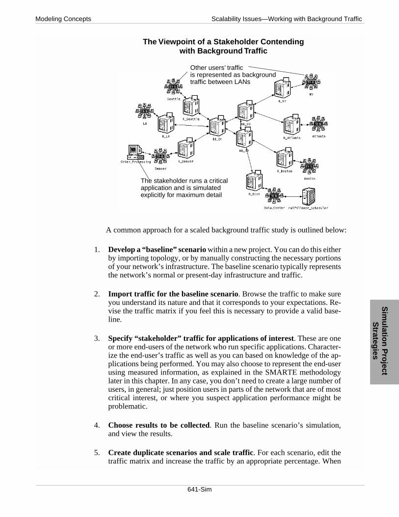
641-Sim


imu

lation

Pro

ject S

trategies

A common approach for a scaled background traffic study is outlined below:

1. Develop a “baseline” scenario within a new project. You can do this eitherby importing topology, or by manually constructing the necessary portionsof your network’s infrastructure. The baseline scenario typically representsthe network’s normal or present-day infrastructure and traffic.

2. Import traffic for the baseline scenario. Browse the traffic to make sureyou understand its nature and that it corresponds to your expectations. Re-vise the traffic matrix if you feel this is necessary to provide a valid base-line.

3. Specify “stakeholder” traffic for applications of interest. These are oneor more end-users of the network who run specific applications. Character-ize the end-user’s traffic as well as you can based on knowledge of the ap-plications being performed. You may also choose to represent the end-userusing measured information, as explained in the SMARTE methodologylater in this chapter. In any case, you don’t need to create a large number ofusers, in general; just position users in parts of the network that are of mostcritical interest, or where you suspect application performance might beproblematic.

4. Choose results to be collected. Run the baseline scenario’s simulation,and view the results.

5. Create duplicate scenarios and scale traffic. For each scenario, edit thetraffic matrix and increase the traffic by an appropriate percentage. When

The Viewpoint of a Stakeholder Contending with Background Traffic

The stakeholder runs a criticalapplication and is simulated explicitly for maximum detail

Other users’ trafficis represented as backgroundtraffic between LANs

642-Sim


scaling traffic, consider if you wish to scale both background traffic and ex-plicit traffic, or only background traffic. In most cases, scaling just thebackground traffic is desirable, because the traffic increase is due to moreusers appearing in the network, not to increased activity by individual us-ers. The purpose of having explicit traffic in the simulation is to representone or more typical users accurately. Their particular traffic should be neg-ligible when compared to the background traffic. Therefore, not scalingtheir contribution should not significantly dilute the selected scaling factor.

Scaling traffic can be performed via the “Traffic Scaling Factor” Simula-tion attribute. (Recall that simulation attributes are specified under the“Configure Simulation” dialog box in the Project Editor). The “TrafficScaling Mode” simulation attribute determines if you will scale only thebackground traffic, or all traffic (including explicitly modeled applica-tions).

6. Run simulations for the duplicated scenarios. Use the “Compare Re-sults” operation to understand how scaling traffic impacts application per-formance.

Note that if you have purchased the Expert Service Prediction (ESP) option, youmay prefer to use the “Specify Traffic Growth” operation in order to quickly run aseries of scenarios and collate and compare results in a more automated fashion.

Creating Cross Traffic for a Specific Network Element

Certain network components do not provide a “Background Utilization” at-tribute, as do LANs or servers. In particular, as of this printing, router and switchmodels do not allow you to model the effects of additional load based on an attributebelonging to the device itself. However, representing such a load is sometimes nec-essary in order to model the “rest of the network” in terms of its effect on the com-ponent of interest. If the load submitted to this device is known (for example, froma measurement), it is typically preferable to avoid constructing a full model of allother parts of the network.

In the absence of a background utilization attribute on the device of interest, youcan still easily specify the desired volume of traffic flowing through the device ofinterest, as follows:

1. “Sandwich” the device between two routers. In other words, create tworouters with the correct layer 2 technologies to connect to the device of in-terest. For instance, if the device is a router with available Token Ringports, choose two routers that also have Token Ring ports (you can even usethe same router model as the device of interest in this case). Connect eachrouter to the device of interest using a bidirectional point-to-point link.These are “artificial routers”, used only to generate the background loadyou seek to introduce for the device of interest. They represent the “rest ofthe network” from this device’s point of view. You can also use LANs in-stead of routers to represent proxy traffic sources.

643-Sim


imu

lation

Pro

ject S

trategies

2. Determine the background traffic you wish to impose on the device of in-terest. Devices like routers and switches are mostly affected by the numberof packets they process, not the number of bits. Therefore, the volume interms of packets per second is really what matters. This is a number youwill generally obtain from measurement or monitoring tools available inyour environment. It may also be an estimate you have made based on sta-tistics collected from other simulations.

3. Specify the background traffic from one router to the other. Choose eitherrouter as the source and the other as the destination. It does not matterwhich is which since your goal is to make packets flow through the deviceof interest. Go to the traffic browser to specify the desired volume of pack-ets per second flowing through the device. The number of bits per packet isnot as important. Choose a number that represents a typical frame size forthe LAN technology being used to connect the devices.

There is one caveat to the approach above when the device of interest is a router.The issue stems from the fact that certain router models account for concurrent pro-cessing of packets on distinct slots. This is controlled by the “IP ProcessingScheme” attribute of the router, which is typically available on advanced models.You will need to know if the device under test is a router which uses a processingscheme which is “Slot Based Processing”. If so, traffic flowing through the routeron certain ports may not affect traffic flowing through on other ports. This dependson whether the ports belong to the same slot of the router. Accordingly, if the back-ground traffic setup between the two “artificial” routers is not on the same slot asother traffic of interest, the desired effect may not be obtained. Therefore, in orderto accomplish sharing of router resources by the background and the explicit traffic,you may have to carefully control the ports that are selected for each of the linksattached to the router. Information on how to do this is provided in the “Workingwith IP” section of this chapter.

Proxy Objects Provide Background Traffic Across a Router

background traffic flows throughRouter 120

644-Sim


A Collection Strategy For Background Traffic

Common sources for background traffic are RMON 2 probes. Using the Multi-Vendor Import product option, you can also import background traffic from Net-work Associates’ Sniffer data if it is saved in ExpertSniffer format. Irrespective ofthe tools you use to collect your information, you will face two other importantquestions:

• Where to Collect?

• When to Collect?

Positioning your Collection Devices

Let us first address the issue of where to collect. First of all, we should ask our-selves where are all the possible places to collect traffic? The assumption madethroughout this section, is that the finest grain location we would consider is theLAN segment. Because of the broadcast nature of local area network traffic on asingle segment, a collection device is able to observe all traffic sent to or from thatsegment. Placing more than one collection device on the same segment would resultin redundant information.

Note that a LAN segment is not the same thing as a LAN. A LAN segment is alayer-2 physical broadcast domain, such as a shared Ethernet segment, or a tokenring, or FDDI segment. If these or other layer 2 technologies are implemented in aswitched environment, then each port of a switch corresponds to a distinct segment,because traffic sent on one port of the switch is not observed by stations accessiblevia the other ports of the switch. In VLAN environments, broadcast domains maybe defined logically, but these do not qualify as segments, since again, the switchesthat implement the VLANs selectively transfer traffic to their different ports.

Our objective is to build a “traffic matrix” to summarize all traffic on the net-work of interest over a period of time. Therefore, we need to ensure that any rele-vant traffic is observed by at least one collection device; otherwise it will not beaccounted for. Doing this as efficiently as possible requires some knowledge of thetraffic patterns. For example, in the scenario below, we may have prior knowledgethat A and B send traffic to and from one another but send relatively insignificanttraffic to C and D. And assume a similar statement could be made about traffic be-tween C and D being exclusive with respect to A and B. Then, we could achievecollection of all inter-segment traffic with just two collection devices, as shown.

645-Sim


imu

lation

Pro

ject S

trategies

We can achieve this goal because all traffic from A to B must cross segment Band similarly for C with respect to D. In other words, in evaluating traffic volumebetween two segments, it does not matter on which of the two segments the collec-tion device is positioned: in either case, the traffic will flow through it. So, whichtraffic flows are not measured with the two collection devices placed as shown?Any traffic between A and C is not measured, because neither has any collectiondevices attached. If this traffic is truly known to be insignificant for the purposes ofour simulation studies, then this traffic collection strategy is acceptable.

The example above serves to illustrate another important point: you must makea decision about whether you wish to capture flows that are internal to segments. Inthe example above, neither A nor B’s internal traffic will be reflected in our trafficmatrix. If you are primarily concerned about backbone (that is, inter-LAN) traffic,then you can safely follow this approach. You may also be selective in collectingintra-LAN traffic for certain segments, but not others. It is important is that you areaware of the consequences of not placing a collection device at a given segment.

Fortunately, in many networks, we can have the type of prior knowledge weneed to efficiently place collection devices. Specifically, highly centralized envi-ronments provide this type of advantage. In highly centralized environments, mosttraffic flows between clients and servers. These servers are concentrated in a rela-tively small number of facilities. Intense local traffic may also be present, but thattraffic is confined to the local area network (for example, for sending jobs to a localprinter). The diagram below illustrates such a network and an effective data collec-tion strategy for characterizing backbone traffic.

Minimizing the Number of Collection Devices

collection device

collection device

captures all C to D andD to C traffic

captures all A to B andB to A traffic

major traffic flow

major traffic flow

646-Sim


If you are unable to leverage prior knowledge of major traffic flows, as in theexamples above, then you may be faced with a more challenging data collection ef-fort, requiring you to perform data collection at each segment. However, for char-acterizing backbone traffic, you may still be able to avoid such widespreadcollection by looking for aggregation points. Typically, these will be at routers orswitches where traffic funnels into the backbone. The diagram below illustrates thisapproach.

Collection in a Primarily Centralized Environment

collection device

collection device

All major flows are to and from the two data centers, so it is sufficient to collect there.

Collection in a Decentralized Environment

collection device

collection device

collection device

collection device

If flows are between all LANs,

collection device

collection cannot be centralized,and must be performed at eachLAN, or at aggregation points,as shown here.

This collection device is requiredbut raises the possibility of redundant data.

647-Sim


imu

lation

Pro

ject S

trategies

Synchronizing Traffic Collection

One fundamental problem affecting collection is that most organizations pos-sess a limited number of collection devices that they can place throughout the net-work. Ideally, one of the approaches discussed above permits performing collectionconcurrently with the number of devices you already have available. However, ifthis is not the case, you do not necessarily have to acquire new devices in order tocollect background traffic.

Your alternative is to collect traffic in phases. For example, if you determinethat you require traffic collection at twenty locations in your network, and you owntwelve RMON-2 probes. Then, you will need two phases of traffic collection. Noindividual location should have its traffic collection repeated, so in this case youwould utilize the output from twelve probes on the first phase, and from eightprobes on the second phase, or some similar partitioning. Relocating probes is typ-ically not a trivial task, so you probably won’t be able to perform both phases oneright after the other. In this case, you could perform the second phase on the follow-ing day, but beginning at the same time of day. The objective is to gather data whilethe network is experiencing similar traffic patterns.

The background traffic system automatically synchronizes all imported trafficinformation to the same time. The first “bucket” of each source of background traf-fic is applied at the same time, and that time is determine by the “Background Traf-fic Start Delay” simulation attribute (set this value in the “Configure Simulation”dialog box).

Managing Redundant Traffic Data

Redundant traffic information typically occurs when collecting in multiplephases. By “redundant”, we mean that two or more distinct traffic profiles are col-lected for the same pair of hosts, but at different times. If this happens for a partic-ular pair of hosts, it is likely to happen for many in your network.

The traffic collection strategies described above favor collection at the “edges”of the network. The edges are the LANs, or the routers associated with those LANs,if you collect aggregated traffic for several LANs at a time. Collecting at the edgeshelps minimize redundant traffic information, when compared with collecting in thecore of the network (that is, within a router mesh connecting the LANs). However,collection in multiple phases, can cause a segment to have its traffic included morethan one phase. Indeed, this is almost impossible to avoid if each segment is beingprobed, or even with aggregation, since a segment will be directly monitored on onecollection phase, but appear as a remote source/destination of traffic, when a datacollection device is applied to other parts of the network in a later phase.

The “Import Traffic” feature allows you to specify how you wish to resolve re-dundant traffic. You are provided with several options: a) use the higher of the col-lected traffic volumes at any point over the collection interval; b) use the sum of thetraffic; and c) use the lowest recorded traffic level. In practice, option (c) is rarelyused, but both options (a), and (b) have appropriate applications. Suppose, for ex-ample, that we have collected traffic twice for a particular pair of hosts, X and Y.

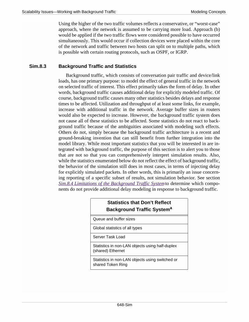
648-Sim


Using the higher of the two traffic volumes reflects a conservative, or “worst-case”approach, where the network is assumed to be carrying more load. Approach (b)would be applied if the two traffic flows were considered possible to have occurredsimultaneously. This would occur if collection devices were placed within the coreof the network and traffic between two hosts can split on to multiple paths, whichis possible with certain routing protocols, such as OSPF, or IGRP.

Sim.8.3 Background Traffic and Statistics

Background traffic, which consists of conversation pair traffic and device/linkloads, has one primary purpose: to model the effect of general traffic in the networkon selected traffic of interest. This effect primarily takes the form of delay. In otherwords, background traffic causes additional delay for explicitly modeled traffic. Ofcourse, background traffic causes many other statistics besides delays and responsetimes to be affected. Utilization and throughput of at least some links, for example,increase with additional traffic in the network. Average buffer sizes in routerswould also be expected to increase. However, the background traffic system doesnot cause all of these statistics to be affected. Some statistics do not react to back-ground traffic because of the ambiguities associated with modeling such effects.Others do not, simply because the background traffic architecture is a recent andground-breaking invention that can still benefit from further integration into themodel library. While most important statistics that you will be interested in are in-tegrated with background traffic, the purpose of this section is to alert you to thosethat are not so that you can comprehensively interpret simulation results. Also,while the statistics enumerated below do not reflect the effect of background traffic,the behavior of the simulation still does in most cases, in terms of injecting delayfor explicitly simulated packets. In other words, this is primarily an issue concern-ing reporting of a specific subset of results, not simulation behavior. See sectionSim.8.4 Limitations of the Background Traffic System to determine which compo-nents do not provide additional delay modeling in response to background traffic.

Statistics that Don’t Reflect Background Traffic Systema

Queue and buffer sizes

Global statistics of all types

Server Task Load

Statistics in non-LAN objects using half-duplex (shared) Ethernet

Statistics in non-LAN objects using switched or shared Token Ring

649-Sim


imu

lation

Pro

ject S

trategies

The fact that certain statistics are not integrated with the background traffic sys-tem does not mean that these statistics are not accurate or meaningful. It simplymeans that these statistics have a different interpretation. Specifically, you shouldinterpret these statistics as reflecting only the activities caused by explicitly simu-lated traffic (for example, traffic generated by application models specified onworkstations and LANs). Finally, as integration of the background traffic systemcontinues, you should check for availability of model library upgrades that wouldchange the list above.

Sim.8.4 Limitations of the Background Traffic System

As a user of the background traffic system, it is important for you to be awareof its limitations. Certain limitations result from the fact that analytical modeling,and therefore hybrid analytical/discrete-event simulation, is not capable of captur-ing all of the same behavior as pure discrete-event simulation. Other limitations willbe overcome with time as enhanced versions of the background traffic system aredeveloped. Despite these existing limitations, which are summarized in this section,the background traffic system is extremely useful, providing an approach to reducesimulation run times while still representing important effects of traffic in the net-work.

• The background traffic system is IP-centric in its current implementa-tion. This means that devices that are the sources and destinations ofbackground traffic must contain the IP protocol. Pure IPX systems, forexample, are not able to act in this capacity. Since IP is essentially the“conduit’ for background traffic information, only intermediate devicesthat support IP or that support IP at lower layers can be affected. Thusa Frame Relay switch that is part of an overall IP infrastructure can car-ry background traffic. However, no background traffic architecture ex-ists at this time for a pure Frame Relay network that does not serve asa bearer of IP traffic.

• Conversation pair traffic only impacts the network, not the server. Gen-erating extra traffic in the network, by scaling the conversation pairtraffic for example, will not create a corresponding increase in task pro-cessing time on the server. This is due to the fact that the backgroundtraffic system is not capable of determining how traffic correlates to

Statistics in non-LAN objects using switched or shared FDDI

Statistics of Protocols at higher layers than IP (for example, TCP, UDP, Applications)

a. check for latest information

Statistics that Don’t Reflect Background Traffic Systema

650-Sim


processing load on servers. It is therefore up to the user to take steps toproperly load the servers. One way to accomplish this is to change theservers’ “Background Utilization” attribute.

• Background traffic is transparent to certain protocol mechanisms.While many protocols in the model library are aware of the backgroundtraffic system, not all of their functionality reflects the presence of theadditional traffic. For example, the weighted fair queuing mechanismof IP does not estimate background traffic’s contribution to queuelengths within each priority, since background traffic does not carrypriority attributes at this time. Additional protocols and mechanismsthat are not sensitive to device/link loads are summarized in the tablebelow. This information is valid as of this printing. As integration of thebackground traffic system continues, you should check for availabilityof relevant model library upgrades.

Models/Mechanisms that Don’t Account for Device/Link Loadsa

a. check for latest information

Non-LAN objects using switched or shared Token Ring

Non-LAN objects using switched or shared FDDI

Non-LAN objects using half-duplex (shared) Ethernet

651-Sim

Modeling Concepts Simulation Methodology for Application Response Time Engineering (SMARTE)S

imu

lation

Pro

ject S

trategies

Sim.9 Simulation Methodology for Application Response Time Engineering (SMARTE)

Application response time is a primary concern in information technology (IT)organizations. Coupled with availability, it is the IT metric most directly associatedwith end-user satisfaction. There are a number of basic of application responsive-ness issues that are typically encountered:

• Investigating poor performance in existing applications. An appli-cation that is already relied upon has exhibited high response timessince its installation, or performance has degraded over time due to fac-tors such as: increased server utilization; decreased server performancedue to new server OS; increased traffic on the network; degraded reli-ability of the network; unfavorable protocol configuration. Simulationprovides an approach for helping you locate the sources of poor perfor-mance and then evaluating solutions.

• Sizing network and computing resources and evaluating networkarchitectures to support critical applications. Network and computerresources, including both physical assets, and leased services, comprisea large portion of IT expenditures. While critical business applicationsmust be supported with adequate infrastructure, you should avoid over-engineering in order to maintain cost-efficiency. Simulation allows youto evaluate your network infrastructure options and make cost-savingchoices with confidence.

• Forecasting application performance under alternative scenarios.For an existing or still-to-be-deployed application, you need to under-stand what performance will be in response to changing conditions.How will the application react to proposed changes in your infrastruc-ture? How will the application perform given a projected profile ofgrowing traffic on the network, and increasing task-load on the serv-er(s). In almost all cases, simulation is the only reliable method to ob-tain such forecasts.

• Understanding new application impact on existing operations. Ifyou are about to deploy a new application that is intensive with respectto the traffic it imposes on the network, or the task-load it submits to theserver(s), you should consider its effect on other critical network appli-cations. Simulation is the most effective tool to provide you with the in-formation you need to avoid adversely affecting other distributedapplications.

In studying any of the above issues, there are two central capabilities that areneeded:

• The ability to characterize the application. This means quantifyingthe behavior of the application with respect to the traffic that it gener-ates on the network, and the utilization in contributes to the server.

652-Sim

Simulation Methodology for Application Response Time Engineering (SMARTE) Modeling Concepts

• The ability to analyze the application in a hypothetical scenario. Inother words, the ability to accurately simulate the application and its en-vironment, as well as changes to each of these.

An OPNET paper titled Simulation Methodology for Application ResponseTime Engineering (SMARTE) describes the SMARTE approach, which you canuse to conduct both of these tasks. The paper is available in two versions: one foruse with the Application Characterization Environment (ACE) module, and anotherfor use without the ACE module. The SMARTE papers are available from our website, www.opnet.com. From the main page, first go to the Support Center, then clickon the Methodologies and Case Studies link.

653-Sim

Modeling Concepts Simulation Methodology for Application Response Time Engineering (SMARTE)S

imu

lation

Pro

ject S

trategies

654-Sim

Simulation Methodology for Application Response Time Engineering (SMARTE) Modeling Concepts

simulation project strategies - suraj @ lumssuraj.lums.edu.pk/~te/simandmod/opnet/09...

Documents