ISR develops, applies and teaches advanced methodologies of design and analysis to solve complex, hierarchical,heterogeneous and dynamic problems of engineering technology and systems for industry and government.

ISR is a permanent institute of the University of Maryland, within the Glenn L. Martin Institute of Technol-ogy/A. James Clark School of Engineering. It is a National Science Foundation Engineering Research Center.

Web site http://www.isr.umd.edu

I RINSTITUTE FOR SYSTEMS RESEARCH

MASTER'S THESIS

Simulation Optimization for Manufacturing System Design

by Rohit KumarAdvisor: Jeffrey W. Herrmann

MS 2003-4

ABSTRACT Title of Thesis: SIMULATION OPTIMIZATION FOR MANUFACTURING

SYSTEM DESIGN

Degree Candidate: Rohit Kumar Degree and year: Master of Science, 2003 Thesis directed by: Associate Professor Jeffrey W. Herrmann Department of Mechanical Engineering

and Institute of Systems Research

A manufacturing system characterized by its stochastic nature, is defined by both

qualitative and quantitative variables. Often there exists a situation when a performance

measure such as throughput, work-in-process or cycle time of the system needs to be

optimized with respect to some decision variables. It is generally convenient to express a

manufacturing system in the form of an analytical model, to get the solutions as quickly

as possible. However, as the complexity of the system increases, it gets more and more

difficult to accommodate that complexity into the analytical model due to the uncertainty

involved. In such situations, we resort to simulation modeling as an effective alternative.

Equipment selection forms a separate class of problems in the domain of

manufacturing systems. It assumes a high significance for capital-intensive industry,

ii

especially the semiconductor industry whose equipment cost comprises a significant

amount of the total budget spent. For semiconductor wafer fabs that incorporate complex

product flows of multiple product families, a reduction in the cycle time through the

choice of appropriate equipment could result in significant profits.

This thesis focuses on the equipment selection problem, which selects tools for

the workstations with a choice of different tool types at each workstation. The objective

is to minimize the average cycle time of a wafer lot in a semiconductor fab, subject to

throughput and budget constraints. To solve the problem, we implement five simulation-

based algorithms and an analytical algorithm. The simulation-based algorithms include

the hill climbing algorithm, two gradient-based algorithms – biggest leap and safer leap,

and two versions of the nested partitions algorithm.

We compare the performance of the simulation-based algorithms against that of

the analytical algorithm and discuss the advantages of prior knowledge of the problem

structure for the selection of a suitable algorithm.

iii

SIMULATION OPTIMIZATION FOR

MANUFACTURING SYSTEM DESIGN

by

Rohit Kumar

Thesis submitted to the Faculty of the Graduate School of the University of Maryland, College Park in partial fulfillment

of the requirements for the degree of Master of Science

2003 Advisory Committee: Associate Professor Jeffrey W. Herrmann, Chairman/Advisor Professor Shapour Azarm Associate Professor Satyandra K. Gupta

iv

© Copyright by

Rohit Kumar

2003

v

DEDICATION

To my parents and grandparents

vi

ACKNOWLEDGEMENTS

First and foremost, I would like to acknowledge the guidance and support

extended by Dr. Jeffrey Herrmann that helped me throughout the two years of my

research work at the University of Maryland, College Park. I cannot thank him enough

for his constructive ideas and criticism, prompt feedback and the patience he showed.

I express my gratitude towards Dr. Fu and Dr. Rubloff, and thank Brian and

Laurent for their valuable inputs regarding the research work that I performed.

I am thankful to the University of Maryland, College Park, the Mechanical

Engineering Department and the Institute of Systems Research for the support they

extended. I also express my appreciation to Dr. Lin and my colleagues in the CIM lab

for the help they provided.

I thank my roommates Jawan, Pyaare, Leader, Jooice, Sreeni, Reekeen, Mahatma

and Aks for standing by me through the last three years.

Last but not the least, I thank my parents, my grandparents and my brother, for

their love, support and most importantly, their belief in me.

DISCLAIMER

This material is based upon work supported by the Semiconductor Research

Corporation and the National Science Foundation (NSF) under grant number DMI

9713720. Any opinions, findings, and conclusions or recommendations expressed in this

material are those of the authors and do not necessarily reflect the views of the NSF.

vii

TABLE OF CONTENTS

1. INTRODUCTION.................................................................................. 1

1.1 Decision variables in a manufacturing system...............................................1

1.2 Complexity of a manufacturing system ...........................................................2

1.3 Optimization of a manufacturing system ........................................................3

1.4 Simulation optimization.......................................................................................3

1.5 Simulation optimization of a manufacturing system....................................4

1.6 Equipment selection problem.............................................................................5

1.7 Objectives of the research ...................................................................................6

1.8 Outline of the thesis ..............................................................................................7

2. LITERATURE REVIEW..................................................................... 9

2.1 Equipment selection problem.............................................................................9

2.1.1 Methods for equipment selection...........................................................................9

2.1.2 Related applications .............................................................................................10

2.2 Simulation-based optimization techniques ...................................................14

2.2.1 Continuous state space.........................................................................................14

2.2.2 Discrete state space ..............................................................................................16

2.3 Summary................................................................................................................23

3. PROBLEM FORMULATION.......................................................... 26

3.1 Problem definition...............................................................................................26

3.2 NP-complete nature of the problem................................................................27

3.2.1 ESP ∈ NP.............................................................................................................28

3.2.2 Integer knapsack problem....................................................................................28

3.2.3 Transforming the integer knapsack problem to ESP ...........................................29

3.3 Sample problem definition................................................................................29

viii

3.4 Summary................................................................................................................31

4. SOLUTION APPROACH.................................................................. 32

4.1 Introduction to the heuristic and the algorithms ..........................................32

4.2 Description of the heuristic ...............................................................................38

4.2.1 Notation................................................................................................................38

4.2.2 Description...........................................................................................................39

4.2.3 Heuristic applied to the sample problem .............................................................40

4.3 Description of the hill climbing algorithm....................................................41

4.3.1 Notation................................................................................................................41

4.3.2 Description...........................................................................................................41

4.3.3 Hill climbing algorithm applied to the sample problem ......................................43

4.4 Description of the biggest leap algorithm .....................................................44

4.4.1 Notation................................................................................................................44

4.4.2 Description...........................................................................................................44

4.4.3 Biggest leap algorithm applied to the sample problem........................................46

4.5 Description of the safer leap algorithm..........................................................48

4.5.1 Notation................................................................................................................48

4.5.2 Description...........................................................................................................48

4.5.3 Safer leap algorithm applied to the sample problem ...........................................51

4.6 Description of NPA-I .........................................................................................52

4.6.1 Notation................................................................................................................52

4.6.2 Description...........................................................................................................53

4.6.3 NPA-I applied to the sample problem .................................................................58

4.7 Description of NPA-II........................................................................................61

4.7.1 Notation................................................................................................................61

4.7.2 Description...........................................................................................................62

4.7.3 NPA-II applied to the sample problem ................................................................70

4.8 Description of the analytical algorithm..........................................................75

4.8.1 Notation................................................................................................................75

ix

4.8.2 Description...........................................................................................................76

4.8.3 Analytical algorithm applied to the sample problem...........................................78

4.9 Results for the sample problem........................................................................79

4.10 Summary .............................................................................................................79

5. RESULTS AND DISCUSSION ....................................................... 80

5.1 Experimental design ...........................................................................................80

5.1.1 Input template files ..............................................................................................81

5.1.2 Simulation model .................................................................................................83

5.1.3 Output file ............................................................................................................84

5.2 Results ....................................................................................................................86

5.2.1 Cost and capacity are not correlated ....................................................................87

5.2.2 Cost and capacity are correlated ........................................................................102

5.2.3 Comparison between Problem Sets 1 and 2.......................................................117

5.3 Summary of the results ....................................................................................118

5.4 Summary..............................................................................................................119

6. SUMMARY AND CONCLUSIONS ............................................ 120

6.1 Conclusions.........................................................................................................120

6.2 Contributions ......................................................................................................122

6.3 Limitations ..........................................................................................................124

6.4 Future work.........................................................................................................125

APPENDIX .............................................................................................. 126

1. Description of the algorithms ...........................................................................126

1.1 Notation.................................................................................................................126

1.2 Description............................................................................................................127

2. Experiments...........................................................................................................129

3. Results.....................................................................................................................130

BIBLIOGRAPHY................................................................................... 134

x

LIST OF TABLES

3.1 Tool costs Cij………………………………………………………………. 30

3.2 Tool capacities µij.…………………………………………………………. 30

4.1 Tool capacity per tool cost Uij……………………………………………... 40

4.2 Ui* and yi………………………………………………………………….... 40

4.3 Number of Tijs bought by the heuristic (Xij0)…………………………….… 41

4.4 Hill climbing algorithm: cycle time values and the tool configuration before and after the iteration……………………………………………….

43

4.5 Biggest leap algorithm: cycle time and the corresponding gradient values

for the first iteration.……………………………………………………….. 47

4.6 Biggest leap algorithm: data for calculating the new tool configuration …. 47

4.7 Safer leap algorithm: cycle time and the corresponding gradient values for the first iteration.…………………………………………………………...

51

4.8 Safer leap algorithm: information for calculating the new tool

configuration……………………………………………………………… 52

4.9 Tool costs Cij………………………………………………………………. 58

4.10 Tool capacities µij………………………………………………………….. 58

4.11 NPA-I: sequence in which the tools are bought………………………….... 60

4.12 Tool costs Cij………………………………………………………………. 70

4.13 Tool capacities µij………………………………………………………….. 71

4.14 NPA-II: sequence in which the tools are bought…………………………... 73

4.15 Analytical algorithm: sequence in which the tools are bought.………….... 78

4.16 Results of the heuristic and the simulation-based algorithms applied to the sample problem…………………………………………………………….

79

5.1 Results when cost and capacity are not correlated……………………….... 88

5.2 Results when cost and capacity are correlated…………………………….. 103

5.3 Performance of the algorithms under consideration………………………. 119

A1 Results for the problem set………………………………………………… 133

xi

LIST OF FIGURES

4.1 Behavior of hill climbing, biggest leap and safer leap algorithms…….…. 34

4.2(a) NPA – partitioning on tool values for workstation 1…………………….. 36

4.2(b) NPA – partitioning on tool values for workstation 2…………………….. 37

4.3 Solution space for NPA-II………………………………………………... 38

5.1 Comparison of the cost metric at β = 1 and β = 3 respectively…………... 91

5.2 Comparison of the capacity metric at β = 1 and β = 3 respectively……… 94

5.3 Comparison of the cycle time metric at β = 1 and β = 3 respectively……. 96

5.4 Comparison of the simulation metric at β = 1 and β = 3 respectively…… 98

5.5 Comparison of cycle time metric vs. the ratio of capacity and cost metrics at β = 1……………………………………………………………

100

5.6 Comparison of cycle time metric vs. the ratio of capacity and cost

metrics at β = 3…………………………………………………………… 101

5.7 Comparison of the cost metric at β = 1 and β = 3 respectively…………... 106

5.8 Comparison of the capacity metric at β = 1 and β = 3 respectively……… 109

5.9 Comparison of the cycle time metric at β = 1 and β = 3 respectively……. 111

5.10 Comparison of the simulation metric at β = 1 and β = 3 respectively…… 113

5.11 Comparison of cycle time metric vs. the ratio of capacity and cost metrics at β = 1……………………………………………………………

115

5.12 Comparison of cycle time metric vs. the ratio of capacity and cost

metrics at β = 3…………………………………………………………… 116

A1 Average cost metric………………………………………………………. 131

A2 Average cycle time metric………………………………………...……… 132

1

1. INTRODUCTION

This chapter provides an insight into the simulation-based optimization for

discrete event manufacturing systems. We also define the research objective. In Section

1.1, we discuss what the decision variables in a manufacturing system can be. In Section

1.2, we discuss the complexity of a manufacturing system with respect to its stochastic

nature. Section 1.3 provides examples of different objective functions we could optimize

in such a system. In Section 1.4, we present a classification of simulation-based

optimization techniques. Section 1.5 discusses the use of those techniques for optimizing

a manufacturing system. Section 1.6 presents the equipment selection problem as a

separate class of problems in the manufacturing system design. The objectives of this

research are defined in Section 1.7, followed by a brief description about each of the

subsequent chapters, in Section 1.8. Whenever we mention optimization problems, we

will be referring to single objective problems.

1.1 Decision variables in a manufacturing system

A manufacturing system has a lot of decision variables that define it. There could

be quantitative decision variables like the number of tools and operators at each

workstation, number of forklifts or other vehicles used for transportation between

workstations and buffer allocation at each workstation, to name a few. Or there could be

qualitative decision variables like the dispatching, routing or scheduling policies, layout

of the manufacturing system, maintenance schedule, and so on and so forth. Depending

upon the kind of questions that a decision-maker would ask in order to design a

2

manufacturing system, the decision variables that play a key role to answer those

questions would vary. Section 1.3 provides examples of such kind of questions.

1.2 Complexity of a manufacturing system

Absence of uncertainty would make the design of a manufacturing system utterly

simple. If the arrival times, processing times, breakdown schedules of the machines,

operator-handling time were deterministic, one could easily determine the values of the

decision variables without much difficulty. Analytical solutions to the problems that a

decision-maker would look for answers to would be quick and accurate. However, the

real life scenario is very different. There exists uncertainty in the arrival times,

processing times, tool breakdowns and machine set-up times for instance. The

complexity of manufacturing systems arises due to this stochastic nature of the processes

in the system and the continual changes that need to be made in the manufacturing line

in the form of addition of new tools to increase capacity, scrapping of old product

families to keep up pace with the market, automating the production line to decrease the

cycle time and the like. Certain properties of the system related to the product or the

process flow when coupled with this uncertainty could increase the complexity

manifold. For instance, semiconductor wafer manufacturing requires repeated layers of

via formation and metalization that necessitate a re-entrant flow routing. The lots of

wafers being routed comprise different product families and yet go through the same

manufacturing line. To add to the complexity, there are constraints on the system. We

mention some of the constraints in the next section.

3

1.3 Optimization of a manufacturing system

There could be several objectives one would like to meet while designing such a

system. For instance, one could find an optimal allocation of resources such as buffers,

to each workstation so as to maximize the throughput of the system. An important

constraint here would be the limited quantity of buffers at each workstation. Another

problem could be to design the layout of the manufacturing line in such a way, so as to

minimize the travel times of the work-in-process (WIP) between workstations. The

constraints could include the shape and the area available for the layout or the number of

resources available to transport the WIP. Another interesting problem could be figuring

out the number of times a defective job should be reworked to maximize the yield. The

obvious constraint here would be that the overall cost of reworking, should never exceed

or be equal to the benefit we reap out of the improved yield. The optimization problem

that we study is the equipment selection problem, discussed in Section 1.6.

1.4 Simulation optimization

Simulation modeling is an effective tool to model, analyze and optimize systems.

It is particularly useful in predicting the behavior of systems with an inherent stochastic

nature, hence the term simulation-based stochastic optimization. Based on the nature of

the decision space, such optimization problems could be categorized as continuous or

discrete.

The decision variables for continuous optimization problems are continuous in

nature. Such problems are solved using techniques such as stochastic approximation

methods, response surface methodology and sample path optimization, besides the

4

gradient estimation techniques that include finite difference estimation, perturbation

analysis, likelihood ratio method and frequency domain analysis.

The decision variables for discrete optimization problems are discrete in nature.

Although the gradient estimation techniques mentioned above, have been applied to

discrete optimization problems, there also exist discrete random and non-random search

methods that are applicable to such problems. Stochastic comparison algorithm,

simulated annealing algorithm, stochastic ruler method, multistart algorithm, ordinal

optimization method, nested partitions algorithm, simulated entropy algorithm,

screening, selection and multiple comparison procedures, genetic algorithm, generalized

and ordinal hill climbing algorithms and Andradottir’s algorithms are techniques based

on random search. There are non-random search methods too, like the branch and bound

algorithm and the low dispersion point set method.

We discuss these methodologies in Chapter 2.

1.5 Simulation optimization of a manufacturing system

Manufacturing systems are analyzed as queueing systems, where the entity being

manufactured or processed is considered as a customer and the machine or the operator

handling the entity is considered as the server. The most important characteristic of such

systems is their event-based nature. The state of the system changes only at the

occurrence of an event such as an arrival or departure of an entity, failure of a machine,

completion of inspection by an operator, or other actions. Since the occurrence of such

events takes place at separated points in time, we generally refer to manufacturing

systems as discrete event manufacturing systems.

5

Though there do exist analytical models to analyze manufacturing systems given

their inherent stochastic nature, it becomes increasingly difficult to adjust them or

develop new analytical models to accommodate complex features and enhanced

variability in the system. These could be in the form of a new routing policy or a

preventive maintenance schedule based on uncertain breakdowns of machines. In such

situations it becomes imperative to use simulation-based models with higher flexibility

to get a more accurate picture.

The decision variables in a manufacturing system discussed earlier in Section

1.2, are generally discrete in nature (unless we are trying to optimize a particular process

along the manufacturing line that is dependent on a continuous parameter such as

temperature or the rate of deposition of a thin-film material). Hence the techniques used

for optimizing a manufacturing system are based on simulation-based discrete stochastic

optimization methodologies, due to the discrete solution space over which we try to

optimize the performance of the system.

1.6 Equipment selection problem

Equipment selection and resource allocation problems form a separate class of

problems in the domain of manufacturing systems design. They deal with the optimal

allocation of machines to workstations in a manufacturing system. Allocation and

selection of tools in manufacturing systems is a widespread problem in manufacturing

plants, especially for sub-systems like Flexible Manufacturing Systems (FMS) and

cellular manufacturing systems. These problems have been addressed using analytical

models, queueing theory and deterministic programming techniques like integer

6

programming. The machine allocations were done with specific objectives like

minimizing WIP, maximizing throughput and minimizing cost. The complexity of the

models was not high enough to necessitate the use of simulation models. For instance,

the servers to be allocated were assumed to be identical. Another classic example of such

types of problems is the buffer allocation problem where a fixed number of buffers must

be allocated over a fixed number of servers to optimize some performance metric. We

discuss how these problems have been addressed in greater detail in Chapter 2. In

semiconductor wafer fabrication plants, equipment selection is extremely important

because of the high cost of purchasing and operating the equipment. In addition,

reducing cycle time (and WIP) is an important objective that is affected by the

equipment selection decision. Our problem deals with the selection of tools for the

workstations in a manufacturing system given a choice of different tool types at each

workstation. Our objective is to minimize the average cycle time subject to the

constraints on the throughput and the budget available.

1.7 Objectives of the research

This research considers the equipment selection problem with our goal being the

minimization of the average cycle time. We present five different simulation-based

stochastic optimization algorithms and observe their behavior with respect to the quality

of solution and the number of simulations each algorithm requires. Their performance is

then compared with that of an analytical algorithm, which we developed as a benchmark.

The first algorithm is similar to the generalized hill climbing (GHC) algorithm

described by Sullivan and Jacobson [1]. We search the neighboring discrete space and

7

estimate the function value at the selected points. However, our approach enumerates all

the neighboring points whereas GHC selects one neighboring point at random. Further,

we do not accept any bad moves whereas GHC could.

The next two algorithms are based on gradient-estimation methods. The gradient

values are estimated using finite differences as in the Kiefer and Wolfowitz [2]

approach. However, the perturbation size in our case is taken as one due to the discrete

nature of the problem whereas Kiefer and Wolfowitz take it to be infinitesimally small.

We also developed two simulation-based stochastic algorithms, which are

different implementations of the nested partitions algorithm, proposed by Shi and

Olafsson [3]. The difference in the two implementations lies in the way we partition the

solution space, to narrow it down through the selection of the most promising region at

the end of each iteration.

The analytical algorithm that we developed is based on the queueing theory. It

makes use of the M/M/m queueing model to find out the average cycle time value. We

use the results of this algorithm as a benchmark to compare the performance of the

simulation-based algorithms that we implemented.

1.8 Outline of the thesis

The thesis is organized as follows. Chapter 2 presents a literature survey and

discusses the equipment selection problem and the simulation-based stochastic

optimization algorithms, applied to discrete event manufacturing systems. Chapter 3

formulates the equipment selection problem, specifying the objective function,

constraints and the decision variables. A sample problem is also defined at the end of the

8

chapter to explain the implementation of our algorithms. Chapter 4 defines a heuristic

(whose result is used as the starting point for the hill climbing, and the gradient-based

algorithms) along with the simulation-based algorithms and the analytical algorithm.

Their implementation is described through the sample problem defined in Chapter 3.

Chapter 5 describes our simulation model and the set-up of our experiments. It defines

the performance metrics based on which we compare the behavior of all the simulation-

based algorithms with the performance of the analytical algorithm. We discuss the

results we obtained. Chapter 6 concludes the thesis, summarizing the results and

discussing the contributions, limitations and the future work, pertaining to the research

we conducted.

9

2. LITERATURE REVIEW

This chapter reviews the research work that has been conducted so far, in the

field of equipment selection and simulation optimization as applied to the discrete event

manufacturing systems. Section 2.1 provides a general review of the equipment selection

and other related problems. Section 2.2 reviews simulation optimization for both the

continuous and discrete state space. We specifically mention the research that has been

done, related to hill climbing, gradient-based and nested partitions methods.

2.1 Equipment selection problem

In the domain of discrete event manufacturing systems, many types of

optimization problems have been discussed, where the performance measures generally

include the mean cycle time, average work-in-process (WIP) at the tool groups,

throughput and tool utilization levels. Equipment selection and resource allocation

problems form a separate class under this domain.

2.1.1 Methods for equipment selection

Compared to the resource allocation class of problems, the problems related to

equipment selection have received less attention. Bretthauer [4] addresses capacity

planning in manufacturing systems by modeling them as a network of queues. Assuming

a single server at each node, a branch-and-bound algorithm is presented to find a

minimum cost selection of capacity levels from a discrete set of choices, given a

constraint on the WIP. Swaminathan [5] provides an analytical model for procurement of

10

tools for a wafer fab incorporating uncertainties in the demand forecasts. The problem is

modeled as a stochastic integer programming with recourse, and the objective is to

minimize the expected stock-out costs due to lost sales across all demand scenarios.

Considering only one tool type per workstation, the first stage variables - the number of

tools procured, are decided before the demand occurs. The second stage variables

determine the allocation of different wafer types to different tools in each demand

scenario, after the demand is realized. Swaminathan [6] presents a more generalized

model where one can model the allocations of each wafer type to the different tools.

Further, a multi-period model is considered to capture changes in demand during the life

of a product. Connors, Feigin and Yao [7] perform tool planning for a wafer fab using a

queueing model, based on a marginal allocation procedure to determine the number of

tools needed to achieve a target cycle time with the objective of minimizing overall

equipment cost. Assuming identical tools at each tool group, their model incorporates

detailed analysis of scrap and rework to capture the effects of variable job sizes on the

workload and on the utilization of tool groups, and careful treatment of “incapacitation”

events that disrupt the normal process at tools.

In the equipment selection problem that we consider, there exist a number of tool

types from which one could select the tools, for a particular workstation.

2.1.2 Related applications

We now review, some of the problems pertaining to the allocation of buffers and

resources, and the methods applied to solve them.

11

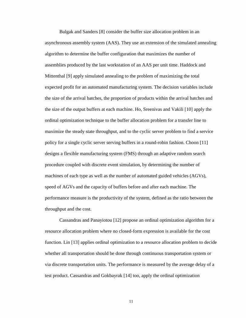
Bulgak and Sanders [8] consider the buffer size allocation problem in an

asynchronous assembly system (AAS). They use an extension of the simulated annealing

algorithm to determine the buffer configuration that maximizes the number of

assemblies produced by the last workstation of an AAS per unit time. Haddock and

Mittenthal [9] apply simulated annealing to the problem of maximizing the total

expected profit for an automated manufacturing system. The decision variables include

the size of the arrival batches, the proportion of products within the arrival batches and

the size of the output buffers at each machine. Ho, Sreenivas and Vakili [10] apply the

ordinal optimization technique to the buffer allocation problem for a transfer line to

maximize the steady state throughput, and to the cyclic server problem to find a service

policy for a single cyclic server serving buffers in a round-robin fashion. Choon [11]

designs a flexible manufacturing system (FMS) through an adaptive random search

procedure coupled with discrete event simulation, by determining the number of

machines of each type as well as the number of automated guided vehicles (AGVs),

speed of AGVs and the capacity of buffers before and after each machine. The

performance measure is the productivity of the system, defined as the ratio between the

throughput and the cost.

Cassandras and Panayiotou [12] propose an ordinal optimization algorithm for a

resource allocation problem where no closed-form expression is available for the cost

function. Lin [13] applies ordinal optimization to a resource allocation problem to decide

whether all transportation should be done through continuous transportation system or

via discrete transportation units. The performance is measured by the average delay of a

test product. Cassandras and Gokbayrak [14] too, apply the ordinal optimization

12

technique for the resource allocation problem, to minimize the average cycle time.

Hillier and So [15] address the server and work allocation problem for production line

systems through the classical model for a system of finite queues in series, to maximize

the throughput. Andradottir and Ayhan [16] determine the optimal dynamic server

assignment policy for tandem systems with a generalized number of servers and stations,

to obtain optimal long-run average throughput. Palmeri and Collins [17] address the

minimum inventory variability policy as one alternative to optimizing resource

scheduling, which focuses on line balancing to reduce the WIP variability resulting in a

reduction in the mean cycle time. Dumbrava [18] attempts to emphasize the benefit of

simulation in resource allocation and capacity design of FMS. The number of machines

in each group is determined to minimize the capacity of the group buffers, minimize the

WIP, and obtain a good compromise between the number of machines and the

productivity obtained. Shanthikumar and Yao [19] address the problem of allocating a

given number of identical servers among the work centers of a manufacturing system by

formulating it as a non-linear integer program. The objective is to maximize the

throughput. Frenk et al. [20] present improved versions of a greedy algorithm for the

machine allocation problem, to achieve a minimum-cost configuration while minimizing

the WIP. Bermon, Feigin and Hood [21] formulate the capacity allocation problem as a

simple, linear programming based method to optimize product mix, subject to capacity

constraints. The objective is to maximize the profit. Bhatnagar et al. [22] formulate fab-

level decision making as a Markov decision problem and address the issues as when to

add additional capacity and when to convert from one production type to another based

on the changing demand. He, Fu and Marcus [23] apply a simulation-based approach to

13

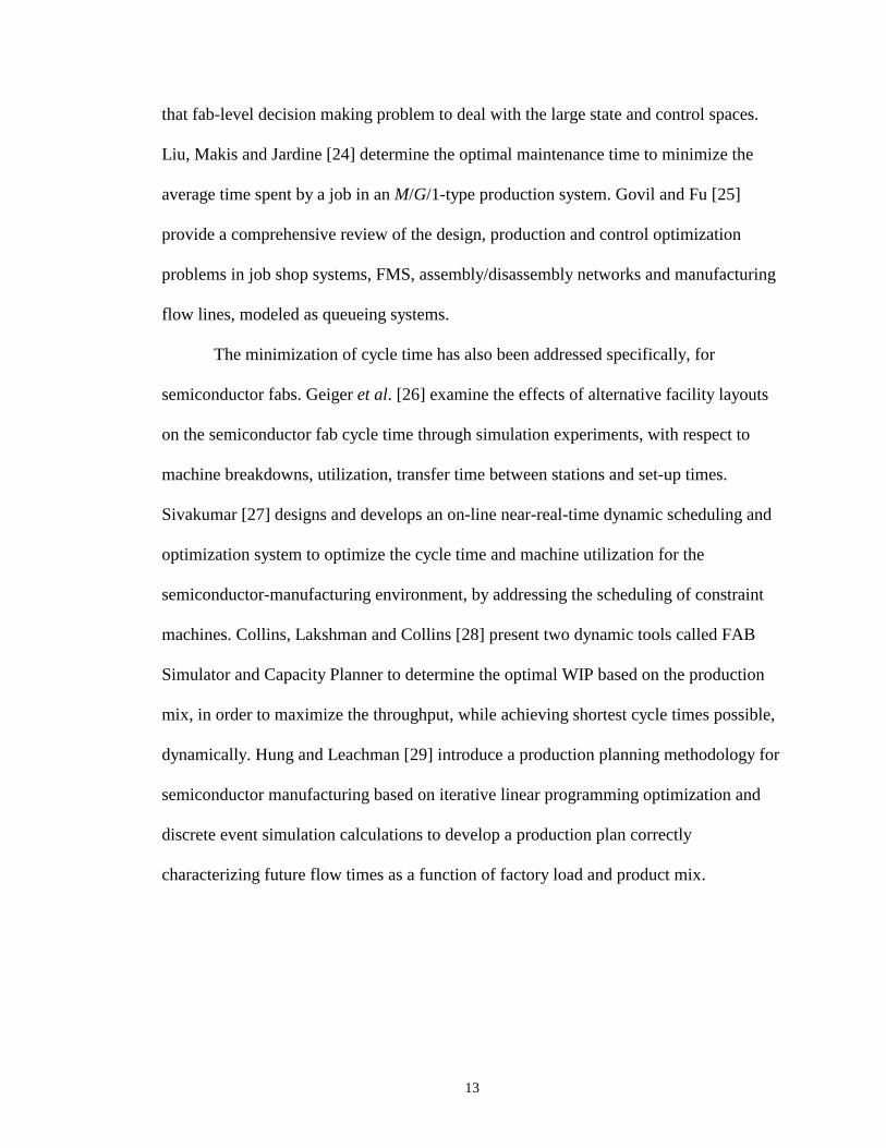
that fab-level decision making problem to deal with the large state and control spaces.

Liu, Makis and Jardine [24] determine the optimal maintenance time to minimize the

average time spent by a job in an M/G/1-type production system. Govil and Fu [25]

provide a comprehensive review of the design, production and control optimization

problems in job shop systems, FMS, assembly/disassembly networks and manufacturing

flow lines, modeled as queueing systems.

The minimization of cycle time has also been addressed specifically, for

semiconductor fabs. Geiger et al. [26] examine the effects of alternative facility layouts

on the semiconductor fab cycle time through simulation experiments, with respect to

machine breakdowns, utilization, transfer time between stations and set-up times.

Sivakumar [27] designs and develops an on-line near-real-time dynamic scheduling and

optimization system to optimize the cycle time and machine utilization for the

semiconductor-manufacturing environment, by addressing the scheduling of constraint

machines. Collins, Lakshman and Collins [28] present two dynamic tools called FAB

Simulator and Capacity Planner to determine the optimal WIP based on the production

mix, in order to maximize the throughput, while achieving shortest cycle times possible,

dynamically. Hung and Leachman [29] introduce a production planning methodology for

semiconductor manufacturing based on iterative linear programming optimization and

discrete event simulation calculations to develop a production plan correctly

characterizing future flow times as a function of factory load and product mix.

14

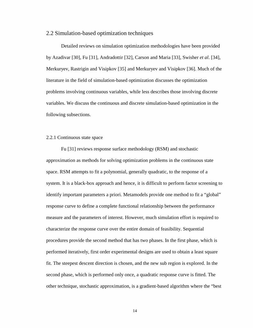
2.2 Simulation-based optimization techniques

Detailed reviews on simulation optimization methodologies have been provided

by Azadivar [30], Fu [31], Andradottir [32], Carson and Maria [33], Swisher et al. [34],

Merkuryev, Rastrigin and Visipkov [35] and Merkuryev and Visipkov [36]. Much of the

literature in the field of simulation-based optimization discusses the optimization

problems involving continuous variables, while less describes those involving discrete

variables. We discuss the continuous and discrete simulation-based optimization in the

following subsections.

2.2.1 Continuous state space

Fu [31] reviews response surface methodology (RSM) and stochastic

approximation as methods for solving optimization problems in the continuous state

space. RSM attempts to fit a polynomial, generally quadratic, to the response of a

system. It is a black-box approach and hence, it is difficult to perform factor screening to

identify important parameters a priori. Metamodels provide one method to fit a “global”

response curve to define a complete functional relationship between the performance

measure and the parameters of interest. However, much simulation effort is required to

characterize the response curve over the entire domain of feasibility. Sequential

procedures provide the second method that has two phases. In the first phase, which is

performed iteratively, first order experimental designs are used to obtain a least square

fit. The steepest descent direction is chosen, and the new sub region is explored. In the

second phase, which is performed only once, a quadratic response curve is fitted. The

other technique, stochastic approximation, is a gradient-based algorithm where the “best

15

guess” of the optimal parameter is updated iteratively based on the estimate of the

gradient of the performance measure, with respect to the parameter. When an unbiased

estimator is used for gradient estimation, the algorithm is referred to as Robbins-Monro

algorithm and when finite difference estimate is used, it is called Kiefer-Wolfowitz

algorithm.

Andradottir [32] focuses on the review of gradient-based techniques for

continuous optimization. Perturbation analysis (PA) and the likelihood ratio (LR)

methods require only a single simulation run to obtain an estimate of the gradient, unlike

the finite difference technique. PA involves tracing the effects of small changes in the

parameter on the sample path. Fu [31] states that wherever infinitesimal perturbation

analysis (IPA, the best known variant of PA) fails, the LR method (also known as the

score function method) works. Azadivar [30] reviews frequency domain analysis as

another method for gradient estimation, where gradients are calculated by noting the

effect of sinusoidal oscillations in the input, on the simulation output function.

Andradottir [32] also reviews sample path optimization, where the expected value of the

objective function is estimated by taking the average of lots of observations. The

objective function is expressed as a deterministic function, based on the sample path

observed on the simulation model, and then the IPA or the LR method is applied.

Swisher et al. [34] classify the continuous parameter case into gradient and non-

gradient-based optimization procedures. The non-gradient-based procedures include the

Nelder-Mead (simplex) method and the Hooke-Jeeves method. Merkuryev and Visipkov

[36] review these two methods. In the Nelder-Mead method, if the objective function is

dependent on k parameters, then k+1 points (a simplex) are generated and the function is

16

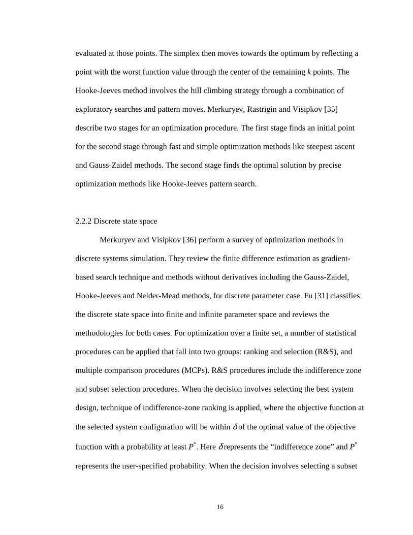
evaluated at those points. The simplex then moves towards the optimum by reflecting a

point with the worst function value through the center of the remaining k points. The

Hooke-Jeeves method involves the hill climbing strategy through a combination of

exploratory searches and pattern moves. Merkuryev, Rastrigin and Visipkov [35]

describe two stages for an optimization procedure. The first stage finds an initial point

for the second stage through fast and simple optimization methods like steepest ascent

and Gauss-Zaidel methods. The second stage finds the optimal solution by precise

optimization methods like Hooke-Jeeves pattern search.

2.2.2 Discrete state space

Merkuryev and Visipkov [36] perform a survey of optimization methods in

discrete systems simulation. They review the finite difference estimation as gradient-

based search technique and methods without derivatives including the Gauss-Zaidel,

Hooke-Jeeves and Nelder-Mead methods, for discrete parameter case. Fu [31] classifies

the discrete state space into finite and infinite parameter space and reviews the

methodologies for both cases. For optimization over a finite set, a number of statistical

procedures can be applied that fall into two groups: ranking and selection (R&S), and

multiple comparison procedures (MCPs). R&S procedures include the indifference zone

and subset selection procedures. When the decision involves selecting the best system

design, technique of indifference-zone ranking is applied, where the objective function at

the selected system configuration will be within δ of the optimal value of the objective

function with a probability at least P*. Here δ represents the “indifference zone” and P*

represents the user-specified probability. When the decision involves selecting a subset

17

of system designs that contain the best solution, the technique of subset selection is

applied, where the selected subset of a specified number of system configurations, will

contain at least one system configuration, such that the objective function at that

configuration will be within δ of the optimal value of the objective function, with a

probability at least P*. The second group of statistical procedures, MCPs, makes

inferences on the performance measure of interest by way of confidence intervals. If the

confidence intervals are not tight enough to make conclusive statements, then an

estimate is made of the number of further replications that would be required so as to

obtain confidence widths at the desired level. Swisher et al. [34] review three main

classes of MCPs: all pairwise multiple comparisons, multiple comparisons with the best

and multiple comparisons with a control. Nelson et al. [37] develop procedures by

combining screening and indifference-zone selection procedures for problems where

R&S would require too much computation to be practical. Such problems arise when the

number of alternative designs is large. Goldsman and Nelson [38] review the screening,

selection and MCPs. Goldsman and Nelson [39] also review various statistical

procedures for selecting the best of a number of competing systems and comment on

how to apply those procedures for use in simulations.

For optimization over an infinite set, there exist random search algorithms.

Carson and Maria [33] review the various heuristic methods, employed for the search.

These include genetic algorithms (GA), evolutionary strategies (ES), simulated

annealing (SA) and Tabu search (TS). Pardalos, Romeijn and Tuy [40] also review these

methods while focusing on the recent developments and trends in global optimization.

GA are noted for robustness in searching complex spaces and are best suited for

18

combinatorial problems. The search starts from an initial population and uses a mixture

of reproduction, crossovers and mutations to create new and hopefully better population.

ES are similar to GA, in that they imitate the principles of natural evolution as a method

to solve parameter optimization problems. The strategy involves the mutation-selection

scheme where one or more parents mutate to produce an offspring and the more

promising candidate becomes the parent for the next iteration. SA is analogous to the

physical annealing process where an alloy is cooled gradually so that a minimal energy

state is achieved. This method can accept bad moves to avoid getting trapped in local

optima. The probability of accepting such bad moves is high when the temperature is

high, and decreases as the temperature reduces. To ensure convergence to a global

optimum, the temperature must be decreased slowly. However, this results in the

evaluation of the objective function at many points. Haddock and Mittenthal [9] deal

with this issue. Gelfand and Mitter [41] modify the SA algorithm to allow for random or

deterministic errors in measurements of the objective function values. Alrefaei and

Andradottir [42] propose a new search algorithm that resembles SA. It uses constant

temperature instead of the decreasing cooling temperature used by SA. Further, it uses

the number of visits to the different states, as the criterion to estimate the optimal

solution. Alrefaei and Andradottir [43] make another modification to SA by using

constant temperature, and selecting the state with the best average estimated objective

function value, obtained from all previous estimates of the objective function values, as

the optimal. TS, also suited for combinatorial problems, maintains a fixed-length list of

explored moves, which represents the Tabu moves. These moves are not allowed at the

19

present iteration, in order to exclude backtracking moves. On the addition of a move to

the Tabu list, the oldest move is removed.

Andradottir [44] proposes a new iterative method to solve discrete stochastic

optimization. The proposed method generates a random walk over the set of feasible

alternatives, and the point visited most often, is shown to be a local optimizer, almost

surely. Yan and Mukai [45] describe the stochastic ruler (SR) method that is related to,

but different from the SA method. While the objective value at a new solution candidate

is compared with that of the current solution candidate in SA, the objective value at a

new solution candidate is compared against a probabilistic ruler in the SR method, where

the ruler’s range covers the range of the observed objective function values. The

convergence is shown to be global. Alrefaei and Andradottir [46] propose another

method based on a modification of the SR method. The new algorithm uses a finite

number of observations for each iteration whereas the SR method uses an increasing

sequence of observations per iteration. The method is shown to converge almost surely,

to the global optimum. Gong, Ho and Zhai [47] propose a method called stochastic

comparison (SC) method that overcomes the limitations of the SA and SR methods. For

SA to work well, it needs a good neighborhood structure. For SR method, if the ruler is

too big, it reduces the sensitivity of the algorithm, whereas if it is too small, it may not

be able to distinguish best solutions from other good solutions. SC, with its roots in the

R&S procedures, eliminates the use of the neighborhood structure and directly compares

the current configuration to a candidate configuration. While comparing the SR and SC

methods, they emphasize that when a good neighborhood structure is available, SR

outperforms the SC algorithm.

20

Other recent developments in the field of discrete parameter simulation

optimization include a new method based on the selection procedures by Futschik and

Pflug [48], in which they construct confidence intervals based on statistical estimates to

select promising subsets with a pre-specified probability of correct selection. Norkin,

Ermoliev and Ruszczynski [49] propose a stochastic version of the branch-and-bound

algorithm in which the search area is divided into subsets. Random upper and lower

bounds for the subsets are calculated with an accuracy depending upon the size of the

subset and the previous values of the objective function estimates. Based on the values

of the bounds, the most promising subset is divided further, while others are neglected.

Ho, Sreenivas and Vakili [10] aim towards finding the good, better or best designs

instead of accurately estimating the performance values of the designs. In other words,

they are interested in the ordinal optimization that is insensitive to noise, rather than the

cardinal optimization. Garai, Ho and Sreenivas [50] propose a hybrid optimization

algorithm that combines adaptive ordinal optimization using GA, with hill climbing. GA

is used to choose the next set of search points from the current set of search points,

which makes the ordinal optimization method adaptive. Hill climbing is used to locate

the best point amongst the points not discarded by the adaptive ordinal optimization

method. Shi and Olafsson [3] describe the nested partitions algorithm (NPA) for

combinatorial problems. The method can be extended to problems where the feasible

region is either countable infinite or uncountable and bounded. The algorithm

concentrates on dividing the search space into sub regions and finding the most

promising region at each iteration, which is then divided further. A nice property of the

algorithm is the ability to backtrack to a larger region. The algorithm is shown to

21

converge globally, with probability one. Shi, Olafsson and Chen [51] propose a new

hybrid optimization algorithm that combines the global perspective of NPA and the local

search capabilities of the GA. It uses the GA search to be able to backtrack quickly from

a region containing a solution better than most, but not all of the other solutions. The

original NPA would take a much longer time to backtrack in such a case. Shi and Chen

[52] combine NPA, ordinal optimization and an efficient simulation control technique

called optimal computing budget allocation (OCBA) to produce a hybrid algorithm for

discrete optimization. OCBA is a ranking and selection method that ensures a larger

allocation of simulation effort amongst the potentially good designs. Sullivan and

Jacobson [1] propose an ordinal hill climbing method based on ordinal optimization and

the generalized hill climbing (GHC) algorithms. GHC seeks to find the optimal design

by allowing the algorithm to visit inferior designs enroute to a globally optimal design.

The ordinal hill climbing algorithm incorporates the design space reduction feature of

ordinal optimization and the global optimization hill climbing feature of GHC

algorithms. Abspoel et al. [53] develop an optimization strategy based on sequential

linearization. In each cycle, a linear approximate sub problem is created and solved. If

the design improves the objective function value, it forms the next cycle’s starting point.

A D-optimal design is used to plan the simulation experiments so that the number of

simulation experiments is kept at a manageable level for increasing number of design

variables. Laguna and Marti [54] describe a training procedure wherein a neural network

filters the solutions likely to perform poorly when the simulations are executed. In other

words, a neural network acts as a prediction model for simulations just as a simulation

acts as a prediction model for a stochastic system.

22

2.2.3 Applications of hill climbing, gradient-based and nested partitions algorithms

We review below, the kind of problems to which hill climbing, gradient-based

and nested partitions algorithms (NPAs) have been applied.

Sullivan and Jacobson [1] apply the ordinal hill climbing to a discrete

manufacturing process design for an integrated blade and rotor geometric shape

component. It considers three manufacturing process design sequences, where each

process has controllable and uncontrollable input parameters associated with it. The cost

function includes the cost of manufacturing, cost penalties for violating process

constraints and cost penalties for not meeting certain geometric and microstructural

specifications. The objective is to identify the best process design sequence, along with

the values of the controllable input parameters so as to minimize the total cost.

Gerencser, Hill and Vago [55] apply a version of stochastic approximation

method for optimizing over discrete sets. They consider the resource allocation problem.

The objective function is the sum of the cost in the form of an expectation incurred by

each user class that depends upon the resources that are allocated to each class.

Cassandras and Gokbayrak [14] convert a discrete resource allocation problem into a

continuous variable surrogate problem in order to be able to obtain sensitivity estimates

via gradient information. The resulting solution after each iteration is mapped back to

the discrete domain. Fu and Healy [56] address the (s,S) inventory control problem using

different methods including a gradient-based algorithm. Whenever the inventory

position falls below the level s, a quantity equal to the difference between S and the

current inventory position is ordered. The objective is to minimize the long-run average

cost per period, which includes the ordering, holding and shortage costs.

23

Shi and Chen [52] develop a new algorithm taking advantage of the global

perspective of NPA and apply it to the buffer allocation problem. Shi, Olafsson and

Chen [51] develop a new algorithm combining NPA and the genetic algorithm for the

product design problem. They maximize the market share by determining the optimal

levels of the attributes of a product. Shi, Chen and Yucesan [57] apply NPA to solve a

buffer allocation problem in supply chain management. Shi, Olafsson and Sun [58]

apply NPA to the traveling salesman problem and emphasize the “parallel” nature of

NPA, suitable for the emerging parallel processing capabilities.

2.3 Summary

This chapter provided a detailed review of the simulation-based optimization

techniques that are used for both continuous and discrete state space. We also provided a

review of the equipment selection and the related problems that have been addressed,

using either queueing models or simulation models for optimization. Law and McComas

[59] mention that one of the disadvantages of simulation historically, is that it was not an

optimization technique. Out of a small number of system configurations that were

simulated, a decision-maker would choose the one that appeared to give the best

performance. Based on the availability of faster computational environments and various

optimization approaches, the situation has changed. Today, simulation software

combined with optimization routines form a powerful tool for many applications. The

goal of such packages is to orchestrate the simulation of a sequence of system

configurations to reach a system configuration that provides an optimal or near optimal

solution.

24

Although there exist many approaches to solve the simulation-based optimization

problems in discrete event manufacturing systems, it is difficult at times to choose

amongst the various available techniques. In other words, it is not easy to identify an

algorithm in advance, with high confidence that it will be the best approach for the

problem at hand. At times, a different implementation of the same algorithm provides

better results. L’Ecuyer, Giroux and Glynn [60] apply different variants of the stochastic

approximation technique to an analytical M/M/1 queueing model to compare them. They

conclude that the gradient estimators through infinitesimal perturbation analysis and

finite differences derivative estimation techniques perform better than likelihood ratio

derivative estimators. Alrefaei and Andradottir [43] compare different variants of the

simulated annealing algorithm through their application on M/M/1 queueing systems.

Based on their choice of values for parameters such as the annealing sequence, the

simulated annealing version they propose gives a better overall performance for a

particular example considered, compared to other versions of the algorithm proposed by

other authors. Sometimes, the structure of the problem might suggest the suitability of

certain algorithms. Gong, Ho and Zhai [47] develop a numerical testbed system and

show that the simulated annealing and stochastic ruler methods outperform the stochastic

comparison method when the search space has a good neighborhood structure. Garai, Ho

and Sreenivas [50] compare adaptive ordinal optimization using genetic algorithm

against hill climbing using the gradient method, through their application on different

queueing models. The comparison is based on the sensitivity to simulation noise. They

show that the adaptive ordinal optimization works better than the pure gradient method

due to its insensitivity to simulation noise. Laguna and Marti [54] compare their scatter

25

search implementation to train a neural network against various training procedures

based on the simulated annealing algorithm. They find that their scatter search

implementation provides solutions comparable to the best methods, but with much less

computational effort. Fu and Healy [56] compare gradient-based, retrospective and

hybrid algorithms while addressing the (s,S) inventory control problem. Their hybrid

algorithm combines the fast convergence of the pure retrospective approach with the low

computational requirement for the gradient search scheme.

This thesis addresses the problem of equipment selection, formulated in the next

chapter, and compares the performance of hill climbing, gradient-based and the nested

partitions algorithms. The suitability of the approaches is discussed at the end, with

respect to the special structure the equipment selection problem has.

26

3. PROBLEM FORMULATION

This chapter defines the equipment selection problem. In section 3.1, we

mathematically formulate the optimization problem, specifying the objective function,

the decision variables and the constraints involved. Section 3.2 proves that our

equipment selection problem is NP-complete. In section 3.3, we define a sample

problem, which is used to describe the heuristic and the algorithms in Chapter 4.

3.1 Problem definition

The problem studied here is one of vital importance, especially to the

semiconductor industry, which invests a great deal of money in equipment. Selecting the

proper set of tools is important for satisfying throughput and budget requirements, and

minimizing average cycle time. We formulate the problem as follows.

The objective is to minimize E[T], the average cycle time of a lot of wafers

through the factory, which is measured using discrete event simulation runs. The

uncertainty in the system lies in the inter-arrival time of the lots and the processing time

of the tools. The factory is a flow shop. Each job (or lot) must visit each workstation in

the same sequence. The travel times between workstations are constant regardless of tool

selection.

The factory has n workstations. Each workstation can have tools of one or more

types. If at ith workstation there are zi types of tools available, then Xij, the number of

tools of type j purchased at each workstation i where i = 1,..., n and j = 1,..., zi form the

27

decision variables. Xij must be a non-negative integer. The total number of decision

variables is p where

The cost of one tool of type j at workstation i is Cij (dollars) and the capacity of

one such tool is µij (wafers per unit time). The decision-maker has a fixed budget of M

(dollars) for purchasing the tools so that the total tool cost cannot exceed M. Also, the

manufacturing system must achieve a throughput of λ (wafers per unit time). If µi is the

capacity at workstation i, then . The constraints can be written as

follows.

for all i, and

Note that for n = 1, our problem reduces to the integer knapsack problem, which we

define later in this chapter.

3.2 NP-complete nature of the problem

Let the number of workstations be 1. We now define an instance of our problem.

Consider a set of tools T at the workstation, comprising different tool types Tj with a cost

Cj, and capacity µj, associated with each tool; a set X specifying the quantity of different

tool types Xj ; a budget constraint M; and a throughput constraint λ. The decision

problem ESP that would correspond to the feasibility of the instance can be stated as

follows.

∑ == iz

j ijiji X1

µµ

λµ >∑=

iz

jijijX

1

MCXn

i

z

jijij

i

≤∑∑= =1 1

1.

n

iip z

==∑

28

Is there a subset such that

and

In the following subsections we prove that ESP is NP-complete. Given an

instance of the integer knapsack problem, we will reduce it to ESP so that a solution to

ESP will exist if and only if there would exist a solution to the integer knapsack

problem.

3.2.1 ESP ∈ NP

Given a solution to the problem ESP, we can easily verify in polynomial time

whether the capacity of the system is greater than λ, and that the total money spent is

less than M. If the solution given to us is where z is the total

number of tool types at the workstation, then the calculations and have a

complexity of θ(z), which is polynomial time.

Hence, ESP belongs to the NP class.

3.2.2 Integer knapsack problem

We pose an instance of the integer knapsack problem below.

A thief robbing a store finds certain items denoted by U. An item u weighs s(u) pounds

and is worth v(u)dollars and exists in multiple quantities. He wants to take at least K

dollars worth of items, but can carry at most B pounds in his knapsack. Mathematically,

it can be expressed as follows (Garey and Johnson [61]).

Consider a finite set U, a “size” and a “value” for each

(where Z denotes the set of integers), a size constraint and a value goal

' ' ' '1 2{ } { , ,..., },j zX X X X=

'X X⊆

'j j

j T

X C M∈

≤∑ ' ?j jj T

X µ λ∈

>∑

'j j

j T

X C∈∑ '

j jj T

X µ∈∑

( )s u Z+∈

( )v u Z+∈

u U∈B Z+∈

.K Z+∈

29

The decision problem can be stated in the following way.

Is there an assignment of a non-negative integer c(u) to each such that

and

3.2.3 Transforming the integer knapsack problem to ESP

Given an instance of the integer knapsack problem, we now create an instance of

ESP. Let Cu = s(u) and µu = v(u), for each Further, let M = B, and λ = K-1. Is there

an assignment of a non-negative integer Xu to each tool of type such that

and

Therefore, we find a 1-1 correspondence between the integer knapsack problem

and ESP. If there exists a solution to the integer knapsack problem, then clearly, there

would exist a solution to ESP. And if there exists a solution to ESP, then clearly there

would exist a solution to the integer knapsack problem.

Since the integer knapsack problem has been shown to be NP-complete (Garey

and Johnson [61]), the arguments presented in section 3.2 prove that finding a solution to

ESP is NP-complete too. Hence, we conclude that since the decision version of the

equipment selection problem is NP-complete, the optimization version is at least as hard

as the decision version. Hence our equipment selection problem is NP-complete.

3.3 Sample problem definition

Consider a manufacturing system with n = 2 workstations, with each workstation

i, having zi = 3 types of tools available. The total number of decision variables is p, so

that 2

1 1

3 6.n

ii i

p z= =

= = =∑ ∑

( ) ( ) ?u U

c u v u K∈

≥∑

u U∈

( ) ( )u U

c u s u B∈

≤∑

.u U∈

,u T∈

u uu T

X C M∈

≤∑ ?u uu T

X µ λ∈

>∑

30

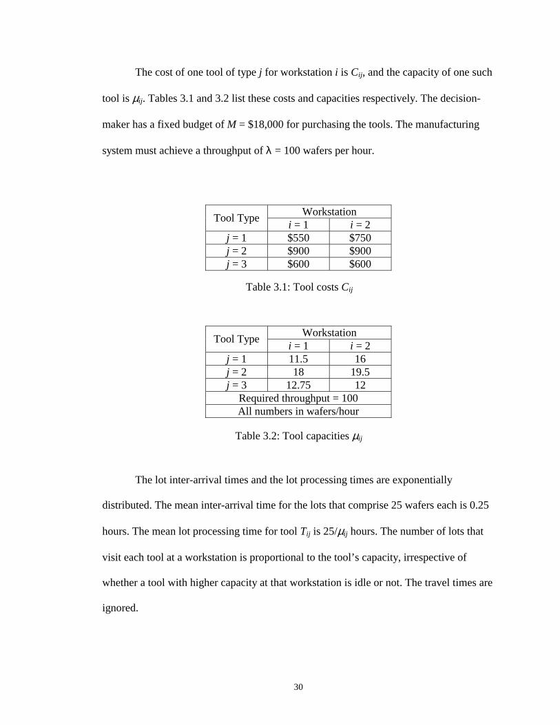
The cost of one tool of type j for workstation i is Cij, and the capacity of one such

tool is µij. Tables 3.1 and 3.2 list these costs and capacities respectively. The decision-

maker has a fixed budget of M = $18,000 for purchasing the tools. The manufacturing

system must achieve a throughput of λ = 100 wafers per hour.

The lot inter-arrival times and the lot processing times are exponentially

distributed. The mean inter-arrival time for the lots that comprise 25 wafers each is 0.25

hours. The mean lot processing time for tool Tij is 25/µij hours. The number of lots that

visit each tool at a workstation is proportional to the tool’s capacity, irrespective of

whether a tool with higher capacity at that workstation is idle or not. The travel times are

ignored.

Workstation Tool Type

i = 1 i = 2 j = 1 $550 $750 j = 2 $900 $900 j = 3 $600 $600

Workstation Tool Type

i = 1 i = 2 j = 1 11.5 16 j = 2 18 19.5 j = 3 12.75 12

Required throughput = 100 All numbers in wafers/hour

Table 3.1: Tool costs Cij

Table 3.2: Tool capacities µij

31

3.4 Summary

This chapter described the equipment selection problem. The next chapter

describes the heuristic and the algorithms that are applied to the sample problem defined

in this chapter.

32

4. SOLUTION APPROACH

This chapter provides a detailed description of the heuristic and all the algorithms

that we have implemented to tackle the problem defined in Chapter 3. Section 4.1

provides an introduction to the heuristic and the algorithms, which are later described in

Sections 4.2 - 4.8. Section 4.2 describes the heuristic. Sections 4.3 - 4.8 describe the hill

climbing, biggest leap, safer leap, nested partitions-I, nested partitions-II and the

analytical algorithms respectively. We also show how the heuristic and the algorithms

are implemented on the sample problem defined in Chapter 3. Section 4.9 reports the

results for that sample problem.

4.1 Introduction to the heuristic and the algorithms

The budget and throughput constraints bound the set of feasible solutions.

Purchasing too few tools will give insufficient capacity. Purchasing too many tools will

violate the budget constraint. Hence the tools must be selected carefully.

For the gradient-based search algorithms, namely hill climbing, biggest leap and

safer leap algorithms, a heuristic is employed as the first step to find a low-cost, feasible

solution by meeting the throughput requirements. Then the gradient-based search

procedure is applied to find better solutions. The gradient gives us the information about

what tools to add in order to reduce the cycle time the most. The search algorithms that

have been developed, use gradient information to direct the search through the discrete

solution space, always moving to a nearby integer point that is feasible. The gradient

provides the search direction.

33

The gradient estimation uses forward differences to avoid violating the

throughput constraints. For example, if Xij represents the number of tools of type j at the

ith workstation, and Xij = 0 at some point in the iteration, then central differences cannot

be used as cycle time values will have to be estimated at Xij = -1 and Xij = 1. However,

the gradient can always be estimated through forward differences, where cycle time

values are estimated at Xij = x and Xij = x+1, x ≥ 0. The three algorithms proposed for this

type of search are:

Hill climbing algorithm: The search consists of taking very small steps, buying

only one tool at a time, till such point that the average cycle time has been minimized or

the budget has been exhausted.

Biggest leap algorithm: The search consists of taking biggest possible leaps,

buying lots of tools when feasible, till such point that the average cycle time has been

minimized or the budget has been exhausted as in Mellacheruvu [62].

Safer leap algorithm: This is a combination of the hill climbing and the biggest

leap algorithms. The search consists of taking large, but cautious steps, till such point

that the average cycle time has been minimized or the budget has been exhausted.

In all cases, the algorithms consider the average cycle time to be minimized if no

step improves it further, within the precision of the simulation tool.

34

Consider a manufacturing system with two workstations, having one tool type

per workstation. Figure 4.1 describes one of the ways in which the three algorithms

could behave if there was enough money to buy at least five more tools, having already

bought 3 tools, assuming that there is enough scope for improvement in the cycle time.

The hill climbing algorithm buys one tool at a time. The biggest leap algorithm buys all

the tools in a single move. The safer leap algorithm takes big, but cautious steps. The

solution in the end may differ as can be seen.

The other kind of search procedure used is the nested partitions algorithm (NPA),

which employs a random search. This procedure does not build up on the low-cost,

feasible solution provided by the heuristic.

Figure 4.1: Behavior of hill climbing, biggest leap and safer leap algorithms

35

The solution space is partitioned into several regions, and solution points are

sampled from each region using a random sampling scheme. The best estimated

objective function value forms the criterion for selecting the most promising region,

which is then, partitioned further. Sampling from the region that surrounds the most

promising region allows escaping local optimums by backtracking to a larger region that

would include the current most promising region. Two versions of NPA (NPA-I and

NPA-II) were developed for our problem. They differ in the way the solution space is

partitioned.

NPA-I: The search partitions the solution space based on the tool values of each

and every existing tool type. Therefore the depth of partitioning (or the number of times

the solution space will have to be partitioned) will be equal to the sum of the different

tool types at each workstation. As we go deeper and deeper in the partitioning process,

we keep on fixing the tool values for those tools that have been partitioned on. These

tool values will be the final ones, unless the procedure backtracks at some later stage in

the partitioning process.

NPA-II: This search deals with a solution space that consists of only one tool

type per workstation. It partitions the solution space in two steps. In the first phase of

partitioning (primary phase), it fixes the tool type that is found to be the most promising,

for each workstation. In the second phase of partitioning (secondary phase), it fixes the

tool values for those chosen tool types. The secondary phase is similar to NPA-I, except

that the input to NPA-I would consist of only one tool type for each workstation. The

depth of partitioning in NPA-II equals twice the number of workstations (for each phase

of partitioning, the depth equals the number of workstations). There could exist a

36

possibility of backtracking from a secondary depth level (secondary node) to a primary

depth level (primary node).

Consider the same manufacturing system with two workstations, having one tool

type per workstation. Figure 4.2 describes the way NPA would work. To begin with, we

would partition the solution space on the tool values for the first workstation. The lines

L1, L2,…,L5 in Figure 4.2(a) represent the solution subspace for which the tool values

for the first workstation are 1,2,…,5 respectively. The bold line L4 indicates the most

promising region after the sampling has been done.

Now, with tool value at first workstation as 4, we partition on the tool values of

the second workstation. The points on the line L4 in Figure 4.2(b) indicate the solution

Figure 4.2(a): NPA – partitioning on tool values for workstation 1

37

subspace at the second depth level. All possible solutions that do not lie on the line L4

form the surrounding region. If the best solution is found on the line L4, the procedure

terminates, returning that solution as the final result, otherwise we backtrack and

partition on the tool values for the first workstation.

If the first workstation had two tool types, then NPA-I would partition on the tool

values of both the tool types at first workstation, and on the tool type at the second

workstation in a similar manner as shown above. NPA-II however, would first partition

to select the most promising tool type, before partitioning to select the tool values. The

partitioning for primary phase would look for the solution subspaces on the X and Y

axes only, as shown in Figure 4.3 (solutions with single tool type per workstation).

Figure 4.2(b): NPA – partitioning on tool values for workstation 2

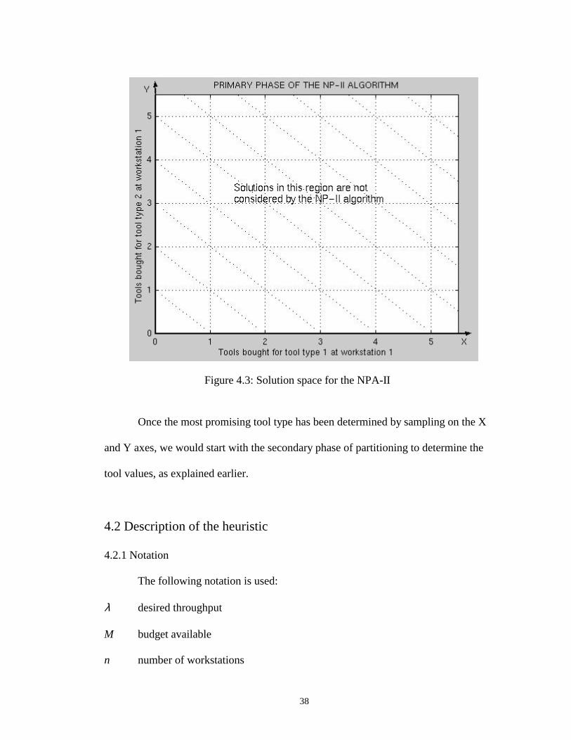
38

Once the most promising tool type has been determined by sampling on the X

and Y axes, we would start with the secondary phase of partitioning to determine the

tool values, as explained earlier.

4.2 Description of the heuristic

4.2.1 Notation

The following notation is used:

λ desired throughput

M budget available

n number of workstations

Figure 4.3: Solution space for the NPA-II

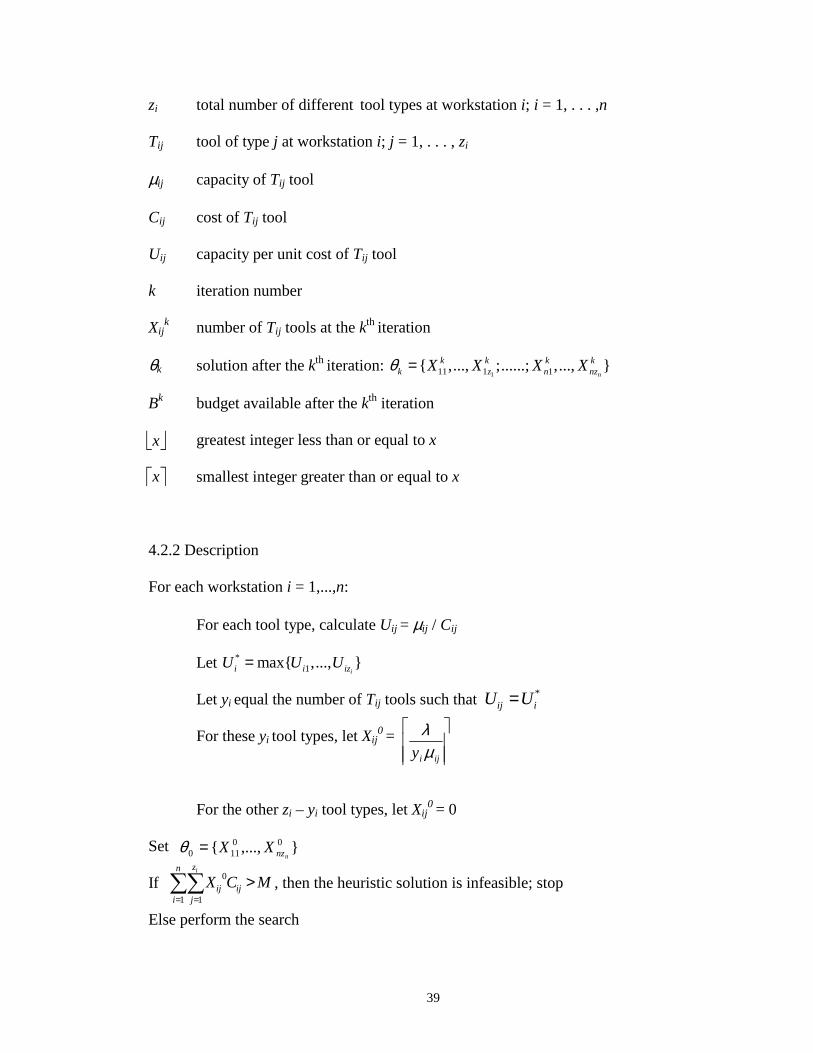
39

zi total number of different tool types at workstation i; i = 1, . . . ,n

Tij tool of type j at workstation i; j = 1, . . . , zi

µij capacity of Tij tool

Cij cost of Tij tool

Uij capacity per unit cost of Tij tool

k iteration number

Xijk number of Tij tools at the kth iteration

θk solution after the kth iteration:

Bk budget available after the kth iteration

greatest integer less than or equal to x

smallest integer greater than or equal to x

4.2.2 Description

For each workstation i = 1,...,n:

For each tool type, calculate Uij = µij / Cij

Let

Let yi equal the number of Tij tools such that

For these yi tool types, let Xij0

=

For the other zi – yi tool types, let Xij0

= 0

Set

If , then the heuristic solution is infeasible; stop

Else perform the search

*iij UU =

∑∑= =

>n

i

z

jijij MCX

i

1 1

0

x

x

ijiy µλ

},...,{ 00110 nnzXX=θ

111 1 1{ ,..., ;......; ,..., }n

k k k kk z n nzX X X Xθ =

*1max{ ,..., }

ii i izU U U=

40

Note that at the end of the heuristic, remaining budget is given as

4.2.3 Heuristic applied to the sample problem

First, the capacities per unit cost (Uij) are calculated for each tool. Table 4.1 lists

these.

Workstation Tool Type

i = 1 i = 2 j = 1 8.36 8.53 j = 2 8.00 8.67 j = 3 8.50 8.00

All numbers in 10-4 wafers/hour/dollar

Table 4.2 lists the s and the yis for the two workstations.

Workstation

i = 1 i = 2 U13 U22

yi 1 1

For the tools T13 and T22,

, and

Table 4.3 lists the number of tools bought (Xij) so as to meet the throughput

requirements.

∑∑= =

−=n

i

z

jijij

i

CXMB1 1

00

*iU

*iU

875.12

100013 =

=

=

ijiyX

µλ

65.19

100022 =

=

=

ijiyX

µλ

Table 4.1: Tool capacity per tool cost Uij

Table 4.2: Ui* and yi

41

Workstation Tool Type

i = 1 i = 2 j = 1 0 0 j = 2 0 6 j = 3 8 0

Finally, we check whether the heuristic solution satisfies the budget constraint or not.

Hence

The average cycle time with this configuration of tools is estimated to be 21.09

hours. Having met the throughput and the budget constraints, the search will be

performed next in order to reduce the cycle time as much as possible, utilizing the

remaining budget B0 where B0 = M – 10,200 = $7,800.

4.3 Description of the hill climbing algorithm

4.3.1 Notation

The following notation is used in addition to that of the heuristic:

N number of replications

p total number of tool types =

average cycle time at point Vij obtained by the rth simulation run at the kth

iteration

4.3.2 Description

If there is no , then return θ0 as the final solution

)(ˆ kijr Vf

0BCij ≤

∑ =

n

i iz1

∑∑= =

=≤=+=n

i

z

jijij

i

MCX1 1

000,18200,10)900*6()600*8(

Table 4.3: Number of Tijs bought by the heuristic (Xij0)

0 0 0 0 0 00 11 12 13 21 22 23{ , , ; , , } {0,0,8;0,6,0}.X X X X X Xθ = =

42

Else initialize k = 0; perform the search

Step 1: Neighborhood Search (This step evaluates all the feasible neighbors of the

current solution)

Step 1.1: Increment k by 1

Step 1.2: For each workstation i = 1,...,n:

For each tool type j = 1,...,zi:

Specify neighbor Vijk as:

For each neighbor where , estimate the cycle time of Vijk as

follows:

Note that this will require at most (Np) simulation runs.

Step 2: If for all Tij, then return θk-1; stop

Else continue

Step 3: Solution update

Step 3.1: Choose Vijk that has the minimum

Step 3.2: Update the values of Xijks

Step 3.3: Let θk = Vijk

Step 3.4: Set

Step 3.5: If there is no Tij that has , then return θk; stop

∑=

=N

r

kijrN

kij Vf

NVf

1

^^

)(1

))((

1−≤ kij BC

kij BC ≤

Nk

ijVf ))((^

ijkk CBB −= −1

NkNk

ij fVf ))(())(( 1

^^

−≥ θ

1

1 1 1 1 111 1 1 1{ ,..., ;...; ,..., 1,..., ; ,..., }

i n

k k k k k k k kij z i ij iz n nzV X X X X X X X− − − − −= +

43

Else go to Step 1

4.3.3 Hill climbing algorithm applied to the sample problem

Since C11 = 550 < B0 = 7800, there is at least one Tij such that . Hence,

perform the search. Initialize k = 0.

Step 1:

Step 1.1: Increment k; k = 1

Step 1.2: Table 4.4 lists the cycle times of the corresponding Vij1

Tool θ0 θ1

T11 5.77 0 0 T12 4.86 0 1 T13 5.42 8 8 T21 20.42 0 0 T22 20.34 6 6 T23 20.56 0 0

Cycle Time values in hours

Step 2: Since there is at least one Tij such that , we

continue with the search

Step 3:

Step 3.1: V121 has the minimum

Step 3.2: Table 4.6 shows the updated values of Xij1

Step 3.3: θ1 = V121 = {0,1,8;0,6,0}

0BCij ≤

)(ˆ 1ijVf

NijVf ))(( 1^

NijNij VfVf ))(())(( 0^

1^

<

NijVf ))(( 1^

Table 4.4: Hill climbing algorithm: cycle time values and the tool configuration before and after the iteration

44

Step 3.4:

Step 3.5: Since C11 = 550 < B1 = 6900, there is at least one Tij such that ;

hence go to Step 1

4.4 Description of the biggest leap algorithm

4.4.1 Notation

The following notation is used in addition to that of the heuristic:

N number of replications

p total number of tool types =

c size of the perturbation = 1

average cycle time at point θk obtained by the rth simulation run

eij unit vector in direction ij

gradient vector at point θk normal to the direction ij

ak step size at iteration k

4.4.2 Description

If there is no , then return θ0 as the final solution

Else initialize k = 0; perform the search

Step 1: Gradient estimation

Step 1.1: Increment k by 1

Step 1.2: For each workstation i = 1,...,n:

For each tool type j = 1,...,zi:

∑=

n

iiz

1

0BCij ≤

690090078001201 =−=−= CBB

1BC ij ≤

^

( )r kf θ

^

( )ij kg θ

45

Let

Estimate as follows:

Note that this will require N(p+1) simulation runs.

Step 2: Solution update

Step 2.1: For each workstation i = 1,...,n:

For each tool type j = 1,...,zi:

Let dijk =

If dijk > 0, then set dij

k = 0; this avoids reducing any Xijk

If Cij > Bk-1, then set dijk = 0; this avoids buying any tools that are too

expensive

Step 2.2: If dijk = 0 for all Tij, then return θk-1; stop

Else continue

Step 2.3: Let

Step 2.4: If all = 0, then

Set Xijk = Xij

k-1 + 1 for Tij where dijk is the smallest (most negative)

= Xijk-1 otherwise;

Bk = Bk-1 - Cij

Else

)(^

kijg θ

∑=

−− −+=

N

r

krijkrNkij c

fcef

Ng

1

1

^

1

^^ )()(1

))((θθ

θ

∑ ∑= =

−−=n

iij

z

j

kij

k

k

Cd

Ba

i

1 1

1

kijkda−

},...,1,...,{ 111111

−−−− +=+= k

nzkij

kijk

kij n

XXXceV θ

∑=

−−=N

rkr

kijr fVf

N 11

^^

)()(1 θ

)(^

kijg θ

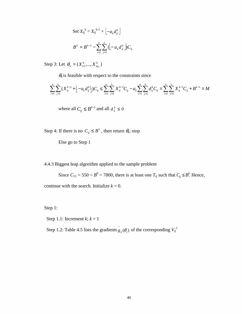
46

Set Xijk = Xij

k-1 +

Step 3: Let

θk is feasible with respect to the constraints since

where all and all

Step 4: If there is no , then return θk; stop

Else go to Step 1

4.4.3 Biggest leap algorithm applied to the sample problem

Since C11 = 550 < B0 = 7800, there is at least one Tij such that . Hence,

continue with the search. Initialize k = 0.

Step 1:

Step 1.1: Increment k; k = 1

Step 1.2: Table 4.5 lists the gradients of the corresponding Vij1

0≤kijd1−≤ k

ij BC

kij BC ≤

kijk da−

1 1 1 1

1 1 1 1 1 1 1 1

( )i i i iz z z zn n n n

k k k k k kij k ij ij ij ij k ij ij ij ij

i j i j i j i j

X a d C X C a d C X C B M− − − −

= = = = = = = =

+ − ≤ − = + = ∑∑ ∑∑ ∑∑ ∑∑

∑∑= =

− −−=n

i

z

jij

kijk

kki

CdaBB1 1

1 )(

},...,{ 11knz

kk n

XX=θ

0BCij ≤

)( 1

^

θijg

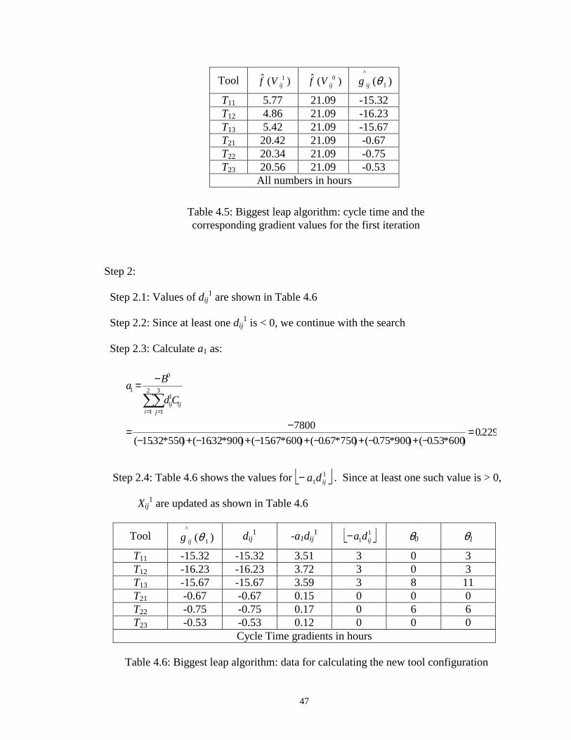
47

Tool

T11 5.77 21.09 -15.32 T12 4.86 21.09 -16.23 T13 5.42 21.09 -15.67 T21 20.42 21.09 -0.67 T22 20.34 21.09 -0.75 T23 20.56 21.09 -0.53

All numbers in hours

Step 2:

Step 2.1: Values of dij1 are shown in Table 4.6

Step 2.2: Since at least one dij1 is < 0, we continue with the search

Step 2.3: Calculate a1 as:

Step 2.4: Table 4.6 shows the values for . Since at least one such value is > 0,

Xij1 are updated as shown in Table 4.6

Tool dij1 -a1dij

1 θ0 θ1

T11 -15.32 -15.32 3.51 3 0 3 T12 -16.23 -16.23 3.72 3 0 3 T13 -15.67 -15.67 3.59 3 8 11 T21 -0.67 -0.67 0.15 0 0 0 T22 -0.75 -0.75 0.17 0 6 6 T23 -0.53 -0.53 0.12 0 0 0

Cycle Time gradients in hours

)(ˆ 1ijVf )(ˆ 0

ijVf )( 1

^

θijg

)( 1

^

θijg 11 ijda−

229.0)600*53.0()900*75.0()750*67.0()600*67.15()900*32.16()550*32.15(

7800

2

1

3

1

1

0

1

=−+−+−+−+−+−

−=

−=∑∑= =i

ijj

ijCd

Ba

11 ijda−

Table 4.5: Biggest leap algorithm: cycle time and the corresponding gradient values for the first iteration

Table 4.6: Biggest leap algorithm: data for calculating the new tool configuration

48

B1 = B0 – (3*550 + 3*900 + 3*600) = 7800 – 6150 = 1650

Step 3:

Step 4: Since C11 = 550 < B1 = 1650, there is at least one Tij such that ; hence

go to Step 1

4.5 Description of the safer leap algorithm

4.5.1 Notation

The following notation is used in addition to that of the heuristic:

N number of replications

p total number of tool types =

c size of the perturbation = 1

average cycle time at point θk obtained by the rth simulation run

eij unit vector in direction ij

gradient vector at point θk normal to the direction ij

ak step size at iteration k

Dk amount spent at the kth iteration

4.5.2 Description

If there is no , then return θ0 as the final solution

Else initialize k = 0; perform the search

∑=

n

iiz

1

0BCij ≤

}0,6,0,11,3,3{},...,{ 123

1111 == XXθ

1BC ij ≤

^

( )r kf θ

^

( )ij kg θ

49

Step 1: Gradient estimation

Step 1.1: Increment k by 1

Step 1.2: For each workstation i = 1,...,n:

For each tool type j = 1,...,zi:

Let

Estimate as follows:

Note that this will require N(p+1) simulation runs.

Step 2: Solution update

Step 2.1: For each workstation i = 1,...,n:

For each tool type j = 1,...,zi:

Let dijk =

If dijk > 0, then set dij

k = 0; this avoids reducing any Xijk

If Cij > Bk-1, then set dijk = 0; this avoids buying any tools that are too

expensive

Step 2.2: If dijk = 0 for all Tij, then return θk-1; stop

Else continue

Step 2.3: Let

)(^

kijg θ

∑=

−− −+=

N

r

krijkrNkij c

fcef

Ng

1

1

^

1

^^ )()(1

))((θθ

θ

∑ ∑= =

−−=n

iij

z

j

kij

k

k

Cd

Ba

i

1 1

1

},...,1,...,{ 111111

−−−− +=+= k

nzkij

kijk

kij n

XXXceV θ

)(^

kijg θ

^ ^

11

1( ) ( )

Nk

r ij r kr

f V fN

θ −=

= −∑

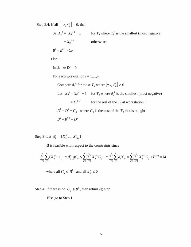
50

Step 2.4: If all = 0, then

Set Xijk = Xij

k-1 + 1 for Tij where dijk is the smallest (most negative)

= Xijk-1 otherwise;

Bk = Bk-1 - Cij

Else

Initialize Dk = 0

For each workstation i = 1,...,n:

Compare dijk for those Tij where > 0

Let Xijk = Xij

k-1 + 1 for Tij where dijk is the smallest (most negative)

= Xijk-1 for the rest of the Tij at workstation i;

Dk = Dk + Cij where Cij is the cost of the Tij that is bought

Bk = Bk-1 – Dk

Step 3: Let

θk is feasible with respect to the constraints since

where all and all

Step 4: If there is no , then return θk; stop

Else go to Step 1

kijkda−

kijkda−

0≤kijd1−≤ k

ij BC

kij BC ≤

1 1 1 1

1 1 1 1 1 1 1 1

( )i i i iz z z zn n n n

k k k k k kij k ij ij ij ij k ij ij ij ij

i j i j i j i j

X a d C X C a d C X C B M− − − −

= = = = = = = =

+ − ≤ − = + = ∑∑ ∑∑ ∑∑ ∑∑

},...,{ 11knz

kk n

XX=θ

51

4.5.3 Safer leap algorithm applied to the sample problem

Since C11 = 550 < B0 = 7800, there is at least one Tij such that . Hence,

continue with the search. Initialize k = 0.

Step 1:

Step 1.1: Increment k; k = 1

Step 1.2: Table 4.7 lists the gradients of the corresponding Vij1

Tool

T11 5.77 21.09 -15.32 T12 4.86 21.09 -16.23 T13 5.42 21.09 -15.67 T21 20.42 21.09 -0.67 T22 20.34 21.09 -0.75 T23 20.56 21.09 -0.53

All numbers in hours

Step 2:

Step 2.1: Values of dij1 are shown in table 4.8

Step 2.2: Since at least one dij1 is < 0, we continue with the search

Step 2.3: Calculate a1 as:

)(ˆ 1ijVf )(ˆ 0

ijVf )( 1

^

θijg

229.0)600*53.0()900*75.0()750*67.0()600*67.15()900*32.16()550*32.15(

7800

2

1

3

1

1

0

1

=−+−+−+−+−+−

−=

−=∑∑= =i

ijj

ijCd

Ba

)( 1

^

θijg

0BCij ≤

Table 4.7: Safer leap algorithm: cycle time and the corresponding gradient values for the first iteration

52

Step 2.4: Table 4.8 shows the values for . Since at least one such value is > 0,

Xij1 are updated as shown in table 4.8. Note that d12

1 is the most negative.

Tool dij1 -a1dij

1 θ0 θ1

T11 -15.32 -15.32 3.51 3 0 0 T12 -16.23 -16.23 3.72 3 0 1 T13 -15.67 -15.67 3.59 3 8 8 T21 -0.67 -0.67 0.15 0 0 0 T22 -0.75 -0.75 0.17 0 6 6 T23 -0.53 -0.53 0.12 0 0 0

Cycle Time gradients in hours

B1 = B0 – C12 = 7800 – 900 = 6900

Step 3: . Note that no tool is added to the second

workstation because all = 0

Step 4: Since C11 = 550 < B1 = 6900, there is at least one Tij such that ; hence,

go to Step 1

4.6 Description of NPA-I

4.6.1 Notation

The following notation is used in addition to that of the heuristic:

Bl remaining budget at the lth partition depth

µi capacity of workstation i, at the current partition depth

F set of those Tij whose Xij are fixed at the current partition depth

11 ijda−

}0,6,0,8,1,0{},...,{ 123

1111 == XXθ

1BC ij ≤

)( 1

^

θijg 11 ijda−

11 ijda−

Table 4.8: Safer leap algorithm: information for calculating the new tool configuration

53

N set of those Tij whose Xij are not fixed at the current partition depth

Ui for Tij N at workstation i

Ui' for all Tij at workstation i

jth highest capacity out of the n workstations

χ

4.6.2 Description

Renumber Tij at each workstation i so that .

Initialize F = { }; N = {(1,1) (2,1) … (n,1) (1,2) (2,2) …… (n,zn)} where (i,j) denotes

the tool Tij.

Step 1: Partitioning

We will assume z1 = z2 =…= zn = z

The depth in the partitioning scheme is governed by the following order:

Calculate ;

The lower and upper bounds on the width at each level of depth are given as:

XhpL = 0 if ∃ j>p : (h,j) N

= otherwise;

min{ }ij

ij

C

µ

jxµ

11 21 1 12 22 2 1 2, ,..., , , ,..., ,......, , ,...,n n z z nzT T T T T T T T T

∈

1 2 ...ii i izµ µ µ≥ ≥ ≥

( , )

lij ij

i j

B M X C∈

= − ∑F

h

hp

λ µµ

−

111 1 1{ ,..., ;......; ,..., }nz n nzX X X X

∈

( , )i ij ij

i j

Xµ µ∈

= ∑F

min{ }ij

ij

C

µ

54

XhpU =

Add (h,p) to F

Step 2: Random Sampling

Let Xij = 0, ∀ (i,j) N

For Xhp = XhpL,…, Xhp

U :

Perform steps 2.1 and 2.2

Step 2.1: Check feasibility:

For each workstation i = 1,...,n:

While (µi ≤ λ), repeat the following loop:

From those (i,j) N , pick a random (i,j) and increment its Xij

Set Bl = Bl - Cij ; µi = µi + µij

If Bl < 0, repeat this step again, choosing different random (i,j)s. If after repeating

a number of times, feasibility is still not obtained, skip the current partition

(represented by the current value of Xhp) as well as the subsequent remaining

partitions (represented by the remaining values of Xhp) at the current depth l.

Step 2.2: Sample a point in the partitioned space:

Pick a uniformly distributed random number R between 0 and Bl

Let P(R) = {(i,j) : (i,j) N , Cij ≤ R}

'

1, 1

max{0,( ) }

min( , )

n hnl

k k ik k h i

hp hp

M

B U U

C

µλ µ

µ= ≠ =

− − −

∑ ∑

∈

∈

∈

55

While P(R) is not empty, repeat the following loop:

Consider those q workstations that have at least one (i,j) P(R)

Arrange these q workstations according to their capacity, such that

Pick a workstation i at rank j, with probability ; let k be the

selected workstation

However, for special cases where capacities of some workstations are

equal, the probability of picking any of these workstations would be the

same. For ex., if , then the probability of

picking workstations

x2, x3 or x4 =

Note that this scheme makes the workstation with lower capacity, more

likely to be selected.

From those (k,j) P(R), randomly pick a (k,j)

Set Xkj = Xkj + 1; R = R - Ckj ; µk = µk + µkj

Step 2.3: Sample a point in the surrounding space:

Let Yij be the number of Tij tools for the surrounding region

Initialize Yij = 0 ∀ (i,j)

Pick a uniformly distributed random number R between and M

Let Q(R) = {(i,j) : Cij ≤ R}

1 2...

qx x xµ µ µ≥ ≥ ≥

2

( 1)

j

q q+

'

1

n

kk

Uλ=∑

∈

1 2 3 4 5...

qx x x x x xµ µ µ µ µ µ> = = > > >

2*(2 3 4) 1*

( 1) 3q q

+ ++

∈

56

While Q(R) is not empty, repeat the following loop:

Consider those q workstations that have at least one (i,j) Q(R)

Arrange these q workstations according to their capacity, such that

Pick a workstation i at rank j, with probability ; let k be the

selected workstation

From those (k,j) in Q(R), randomly pick a (k,j)

Set Xkj = Xkj + 1; R = R- Ckj ; µk = µk + µkj

If, for any workstation i, µi < λ, then discard the sample

Further, if ∀ (i,j) F , Xij = Yij, discard the sample because it does not

belong to the surrounding region

Note that at depth level = 1, there exists no surrounding region.

Step 3: Calculating the promising index

For each sample point in every partitioned region, the value of the objective

function is estimated. The promising index for region r (=1,…,# of partitions) is

given by ,

where is the average cycle time at the ith sample point χ belonging to region r.

The most promising region is taken as the one that has the minimum .

Step 4: Further partitioning or backtracking

If one of the subregions has the best promising index value, that subregion is

partitioned further using the same scheme. However, if the surrounding region looks to

( . .)rP I

ˆ( . .) m in{ ( )}ir rP I f χ=

ˆ ( )ir

f χ

( . .)rP I

2

( 1)

j

q q+

1 2...

qx x xµ µ µ≥ ≥ ≥

∈

∈

57

be the most promising region, then we backtrack to a larger region, using the scheme

described by Shi and Chen [52].

If the fixed components of the best design at the current depth level l are denoted as:

and the fixed components of the best design at the previous depth level l-1 are denoted

as: when p = 1,

otherwise,

then we backtrack to the level that θfixed and θ*fixed have the same components at that

level and above. Hence after backtracking, the fixed components would have the form:

where v < q, or, v = q and u ≤ p-1

Note that in the implementation of NPAs, the best solution at each iteration

always forms a candidate solution for the next iteration, even if we backtrack.

The flow of NPA-I can be described as follows:

While at least one tool N , repeat the following loop:

For width (at each level of depth) = XhpL,…,Xhp

U :

For desired number of samples (= 5, in our implementation):

Randomly sample a point (as described in Steps 2.1 and 2.2)

Estimate the objective function value for the sampled point

For desired number of samples (= 50, in our implementation):

Randomly sample a point in the surrounding region (as described in Step

2.3)

11 21 1 1 2{ , ,..., ,......, , ,..., }, ( 1) 1fixed n q q pqX X X X X X l n q pθ = = − + +

11 21 1 1( 1) 2( 1) ( 1)

* * * * * * *{ , ,..., ,......, , ,..., }n q q n qfixed X X X X X Xθ

− − −=

11 21 1 1 2{ , ,..., ,......, , ,..., }

n v v uvfixed X X X X X Xθ+ + + + + + +=

11 21 1 1 2 ( 1)

* * * * * *{ , ,..., ,......, , ,..., }n q q p q

X X X X X X−

=

∈

58

Estimate the objective function value for the sampled point

If the sample point having minimum objective function value is not in the

surrounding region, then

Remove a tool from N, add it to F, and continue

Else

Backtrack, adjusting the sets F and N accordingly (as described in

Step 4)

4.6.3 NPA-I applied to the sample problem

Tables 4.9 and 4.10 are obtained after renumbering the tools, according to their

capacities. The depth in the partitioning scheme will be governed by the following order:

Workstation Tool Type

i = 1 i = 2 j = 1 $900 $900 j = 2 $600 $750 j = 3 $550 $600

Workstation Tool Type

i = 1 i = 2 j = 1 18 19.5 j = 2 12.75 16 j = 3 11.5 12

Required throughput = 100 All numbers in wafers/hour

11 21 12 22 13 23, , , , ,T T T T T T

Table 4.9: Tool costs Cij

Table 4.10: Tool capacities µij

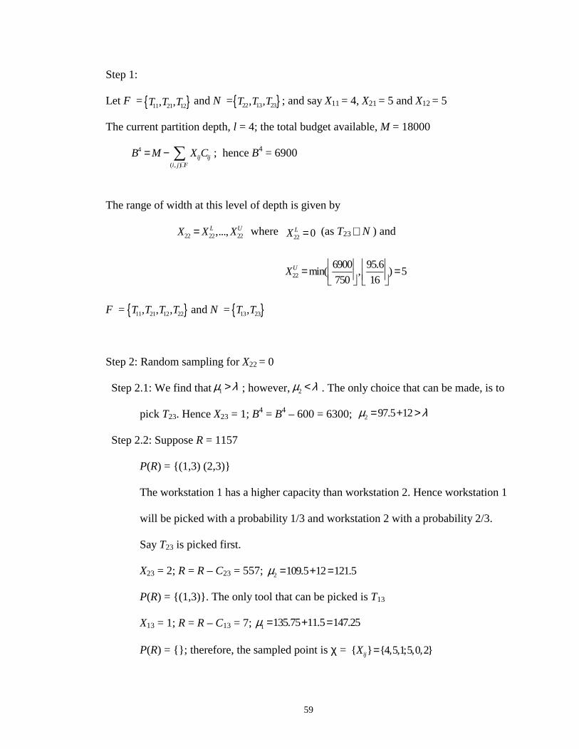
59

Step 1:

Let F = and N = ; and say X11 = 4, X21 = 5 and X12 = 5

The current partition depth, l = 4; the total budget available, M = 18000

; hence B4 = 6900

The range of width at this level of depth is given by

where (as T23 N ) and

F = and N =

Step 2: Random sampling for X22 = 0

Step 2.1: We find that ; however, . The only choice that can be made, is to

pick T23. Hence X23 = 1; B4 = B4 – 600 = 6300;

Step 2.2: Suppose R = 1157

P(R) = {(1,3) (2,3)}

The workstation 1 has a higher capacity than workstation 2. Hence workstation 1

will be picked with a probability 1/3 and workstation 2 with a probability 2/3.

Say T23 is picked first.

X23 = 2; R = R – C23 = 557;

P(R) = {(1,3)}. The only tool that can be picked is T13

X13 = 1; R = R – C13 = 7;

P(R) = {}; therefore, the sampled point is χ =

{ }11 21 12, ,T T T { }22 13 23, ,T T T

22 22 22,...,L UX X X=

{ }11 21 12 22, , ,T T T T { }13 23,T T

1µ λ> 2µ λ<

4

( , )ij ij

i j

B M X C∈

= − ∑F

2 97.5 12µ λ= + >

2 109.5 12 121.5µ = + =

1 135.75 11.5 147.25µ = + =

{ } {4,5,1;5,0,2}ijX =

22

6900 95.6min( , ) 5

750 16UX

= =

22 0LX = ∈

60

We stop here, and continue this procedure to get more samples for this partition.

Thereafter, random sampling for subsequent partitions is performed.

Step 2.3: Surrounding region for the current depth is sampled as follows:

and M = 18000; Suppose R = 12700

Q(R) = {(1,1) (1,2) (1,3) (2,1) (2,2) (2,3)}

Table 4.11 gives the sequence of random selection for this sample

Capacity (wafers / hr)

Prob. of Selection Resulting Choice Seq. #

WS 1 WS 2 WS 1 WS 2 WS Tool

Remaining Budget (R)

1 0 0 0.5 0.5 2 T21 11800 2 0 19.5 0.667 0.333 2 T21 10900 3 0 39 0.667 0.333 1 T11 10000 4 18 39 0.667 0.333 1 T12 9400 5 30.75 39 0.667 0.333 1 T11 8500 6 48.75 39 0.333 0.667 1 T11 7600 7 66.75 39 0.333 0.667 2 T21 6700 8 66.75 58.5 0.333 0.667 2 T23 6100 9 66.75 70.5 0.667 0.333 1 T12 5500 10 79.5 70.5 0.333 0.667 1 T11 4600 11 97.5 70.5 0.333 0.667 2 T21 3700 12 97.5 90 0.333 0.667 2 T21 2800 13 97.5 109.5 0.667 0.333 1 T12 2200 14 110.25 109.5 0.333 0.667 1 T12 1600 15 123 109.5 0.333 0.667 1 T12 1000 16 135.75 109.5 0.333 0.667 2 T22 250 17 135.75 125.5 0.333 0.667

The set Q(R) does not change till the seq. # 16, after which it becomes empty.

The sampled point γ = . From the table, we can see that

'

1

9321.27n

kk

Uλ=

=∑

{ } {4,5,0;5,1,1}ijY =

Table 4.11: NPA-I: sequence in which the tools are bought

61

capacity-feasible solution is obtained. However, the corresponding values of Xij

and Yij ∀ (i,j) F are found to be the same. Therefore this sampled point does

not belong to the surrounding region, and hence is discarded.

Step 3: The cycle time values are calculated for each point sampled in Step 2.

Step 4: Let us say, the best sampled point (with least estimated cycle time value) is

found in the surrounding region: γ = .We find that

and

Therefore, after backtracking, we get ; the partition depth is now set to

2, and the procedure is repeated.

4.7 Description of NPA-II

The tree structure in our NPA-II implementation consists of two kinds of nodes:

primary and secondary. The primary nodes occupy the first few levels of depth of the

tree, and are associated with the identification of the most promising tool types at each

workstation. Secondary nodes are associated with searching for the optimal quantities of

those tool types identified through primary nodes.

The tree structure in the NPA-I implementation involved only the secondary

nodes (the number of such nodes was (nz), the total number of tool types).

4.7.1 Notation

The following notation is used in addition to that of the heuristic:

{4,8,0;4,3,4}

11 21 12 22{ , , , } {4,4,8,3}fixed X X X Xθ = = * * * *11 21 12{ , , } {4,5,5}fixed X X Xθ = =

11{ } {4}fixed Xθ+ += =

∈

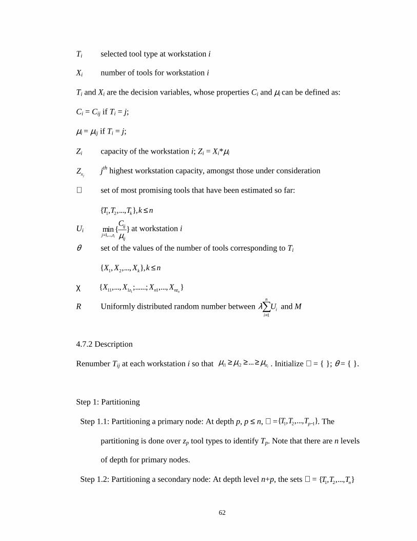
62

Ti selected tool type at workstation i

Xi number of tools for workstation i

Ti and Xi are the decision variables, whose properties Ci and µi can be defined as:

Ci = Cij if Ti = j;

µi = µij if Ti = j;

Zi capacity of the workstation i; Zi = Xi*µi

jth highest workstation capacity, amongst those under consideration

ℑ set of most promising tools that have been estimated so far:

Ui at workstation i

θ set of the values of the number of tools corresponding to Ti

χ

R Uniformly distributed random number between and M

4.7.2 Description

Renumber Tij at each workstation i so that . Initialize ℑ = { }; θ = { }.

Step 1: Partitioning

Step 1.1: Partitioning a primary node: At depth p, p ≤ n, ℑ = . The

partitioning is done over zp tool types to identify Tp. Note that there are n levels

of depth for primary nodes.

Step 1.2: Partitioning a secondary node: At depth level n+p, the sets ℑ =

1,...,min { }

i

ij

j zij

C

µ=

1 2{ , ,..., },kX X X k n≤

1 2{ , ,..., },kT T T k n≤

1 2 1{ , ,..., }pT T T −

1 2{ , ,..., }nT T T

1

n

ii

Uλ=∑

jxZ

1 2 ...ii i izµ µ µ≥ ≥ ≥

111 1 1{ ,..., ;......; ,..., }nz n nzX X X X

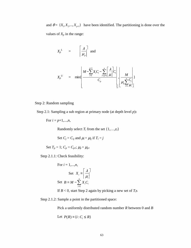
63

and θ = have been identified. The partitioning is done over the

values of Xp in the range:

XpL = and

XpU =

Step 2: Random sampling

Step 2.1: Sampling a sub region at primary node (at depth level p):

For i = p+1,...,n,

Randomly select Ti from the set {1,…,zi}

Set Cj = Cij and µi = µij if Ti = j

Set Tp = 1; Cp = Cp1; µp = µp1

Step 2.1.1: Check feasibility:

For i = 1,...,n,

Set

Set

If B < 0, start Step 2 again by picking a new set of Tis

Step 2.1.2: Sample a point in the partitioned space:

Pick a uniformly distributed random number R between 0 and B

Let

1

1 1

1

min{ , }

p n

i i ii i p i

nip

pi i

M X C CM

CC

λµ

µµ

−

= = +

=

− −

∑ ∑

∑

p

λµ

1 2 1{ , ,..., }pX X X −

ii

Xλµ

=

( ) { : }iP R i C R= ≤

1

n

i ii

B M X C=

= −∑

64

While P(R) is not empty, repeat the following loop:

Consider those q workstations that belong to P(R)

Arrange these q workstations according to their capacity, such that

Pick a workstation i at rank j, with probability ; let k be the

selected workstation

However, for special cases where capacities of some workstations

are equal, the probability of picking any of these workstations

would be the same. For ex., if ,

then the probability of picking workstations x2, x3 or x4 equals

Note that this scheme makes the workstation with lower capacity,

more likely to be selected.

Set Xk = Xk+1; R = R – Ck; Zi = Zi + µi

Let X* = Xp; C* = Cp

For i = 2,...,zp:

Set Tp = i; Cp = Cpi; µp = µpi

Set

Hence we get zp samples whose Ti and Xi are the same for all i≠p, but Xp may be

different as Tp are different.

Step 2.2: Sampling a sub region at secondary node (at depth level n+p):

1 2...

qx x xZ Z Z≥ ≥ ≥

2

( 1)

j

q q+

1 2 3 4 5...

qx x x x x xZ Z Z Z Z Z> = = > > >

2*(2 3 4) 1*

( 1) 3q q

+ ++

* *

( )pp

X CX Round

C=

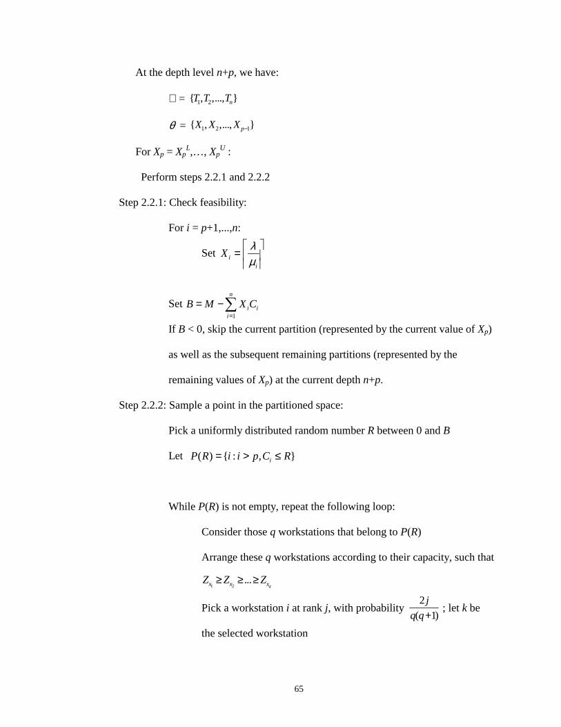
65

At the depth level n+p, we have:

ℑ =

θ =

For Xp = XpL,…, Xp

U :

Perform steps 2.2.1 and 2.2.2

Step 2.2.1: Check feasibility:

For i = p+1,...,n:

Set

Set

If B < 0, skip the current partition (represented by the current value of Xp)

as well as the subsequent remaining partitions (represented by the

remaining values of Xp) at the current depth n+p.

Step 2.2.2: Sample a point in the partitioned space:

Pick a uniformly distributed random number R between 0 and B

Let

While P(R) is not empty, repeat the following loop:

Consider those q workstations that belong to P(R)

Arrange these q workstations according to their capacity, such that

Pick a workstation i at rank j, with probability ; let k be

the selected workstation

1 2 1{ , ,..., }pX X X −

1 2{ , ,..., }nT T T

1 2...

qx x xZ Z Z≥ ≥ ≥

2

( 1)

j

q q+

( ) { : , }iP R i i p C R= > ≤

ii

Xλµ

=

1

n

i ii

B M X C=

= −∑

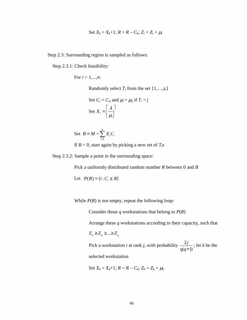
66

Set Xk = Xk+1; R = R – Ck; Zi = Zi + µi

Step 2.3: Surrounding region is sampled as follows:

Step 2.3.1: Check feasibility:

For i = 1,...,n:

Randomly select Ti from the set {1,…,zi}

Set Ci = Cij and µi = µij if Ti = j

Set

Set

If B < 0, start again by picking a new set of Tis

Step 2.3.2: Sample a point in the surrounding space:

Pick a uniformly distributed random number R between 0 and B

Let

While P(R) is not empty, repeat the following loop:

Consider those q workstations that belong to P(R)

Arrange these q workstations according to their capacity, such that

Pick a workstation i at rank j, with probability ; let k be the

selected workstation

Set Xk = Xk+1; R = R – Ck; Zk = Zk + µk

ii

Xλµ

=

( ) { : }iP R i C R= ≤

1 2...

qx x xZ Z Z≥ ≥ ≥

2

( 1)

j

q q+

1

n

i ii

B M X C=

= −∑

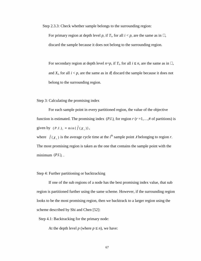
67

Step 2.3.3: Check whether sample belongs to the surrounding region:

For primary region at depth level p, if Ti, for all i < p, are the same as in ℑ ,

discard the sample because it does not belong to the surrounding region.

For secondary region at depth level n+p, if Ti, for all i ≤ n, are the same as in ℑ ,

and Xi, for all i < p, are the same as in θ, discard the sample because it does not

belong to the surrounding region.

Step 3: Calculating the promising index

For each sample point in every partitioned region, the value of the objective

function is estimated. The promising index for region r (r =1,…,# of partitions) is

given by ,

where is the average cycle time at the ith sample point belonging to region r.

The most promising region is taken as the one that contains the sample point with the

minimum .

Step 4: Further partitioning or backtracking

If one of the sub regions of a node has the best promising index value, that sub

region is partitioned further using the same scheme. However, if the surrounding region

looks to be the most promising region, then we backtrack to a larger region using the

scheme described by Shi and Chen [52]:

Step 4.1: Backtracking for the primary node:

At the depth level p (where p ≤ n), we have:

( . .)rP I

ˆ( . .) m in{ ( )}ir rP I f χ=

ˆ ( )ir

f χ

( . .)rP I

χ

68

ℑ =

Let the tool types for the workstations 1,…,p for the best sample in the surrounding

region be represented as:

ℑ * =

If ℑ * ≠ ℑ , then we backtrack to the level k where ℑ * and ℑ would have the same

components at that level and above. After backtracking, we would have

ℑ + = .

Note that for all j ≤ k,

Step 4.2: Backtracking for the secondary node:

At depth level n+p (where p ≤ n), we have:

ℑ =

θ =

Let the best sample in the surrounding region be represented as:

ℑ * =

θ* =

If ℑ * ≠ ℑ , we backtrack using the same scheme as in Step 4.1.

Else if ℑ * = ℑ , then we backtrack to the level where θ* and θ have the same components

at that level and above. After backtracking, we would have

θ+=

Note that for all j ≤ k,

1 2{ , ,..., }, 1

kT T T k p+ + + < −

1 2{ , ,..., }, 1kX X X k p+ + + < −

*j j jT T T+= =

*j j jX X X+= =

1 2 1{ , ,..., }pT T T −

1 2 1

* * *{ , ,..., }p

T T T−

1 2{ , ,..., }nT T T

1 2 1{ , ,..., }pX X X −

1 2

* * *{ , ,..., }n

T T T

1 2 1

* * *{ , ,..., }p

X X X−

69

The flow of NPA-II can be described as follows:

While the set θ is incomplete, repeat the following loop:

If the node is primary, then

For the desired number of samples (= 5, in our implementation):

Randomly sample a point (as described in Step 2.1)

Estimate the objective function value for the sampled point

For the desired number of samples (= 50, in our implementation):

Randomly sample a point in the surrounding region (as described

in Step 2.3)

Estimate the objective function value for the sampled point

If the sample point having minimum objective function value is not in the

surrounding region, then

Add the chosen tool for the workstation that is being partitioned

on, to ℑ

Else

Backtrack, adjusting the set ℑ accordingly (as described in Step 4)

Else if the node is secondary, then

For width (at each level of depth) = XpL to Xp

U :

For the desired number of samples (= 5, in our implementation):

Randomly sample a point (as described in Step 2.2)

Estimate the objective function value for the sampled point

For the desired number of samples (= 50, in our implementation):

70

Randomly sample a point in the surrounding region (as described

in Step 2.3)

Estimate the objective function value for the sampled point

If the sample point having minimum objective function value is not in the

surrounding region, then

Add Xp (tool value corresponding to the tool Tp, for the best

sample found) to θ

Else

Backtrack, adjusting the sets ℑ and θ accordingly (as described in

Step 4)

Adjust the type of node depending on the new depth level

4.7.3 NPA-II applied to the sample problem

Workstation Tool Type

i = 1 i = 2 j = 1 18 19.5 j = 2 12.75 16 j = 3 11.5 12

Required throughput = 100 All numbers in wafers/hour

Table 4.12: Tool costs Cij

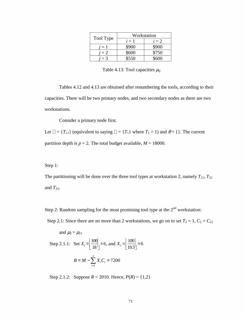
71

Tables 4.12 and 4.13 are obtained after renumbering the tools, according to their

capacities. There will be two primary nodes, and two secondary nodes as there are two

workstations.

Consider a primary node first.

Let ℑ = {T11} (equivalent to saying ℑ = {T1} where T1 = 1) and θ = {}. The current

partition depth is p = 2. The total budget available, M = 18000.

Step 1:

The partitioning will be done over the three tool types at workstation 2, namely T21, T22

and T23.

Step 2: Random sampling for the most promising tool type at the 2nd workstation:

Step 2.1: Since there are no more than 2 workstations, we go on to set T2 = 1, C2 = C21

and µ2 = µ21

Step 2.1.1: Set , and

Step 2.1.2: Suppose R = 2010. Hence, P(R) = {1,2}

Workstation Tool Type

i = 1 i = 2 j = 1 $900 $900 j = 2 $600 $750 j = 3 $550 $600

1

1006

18X

= = 2

1006

19.5X

= =

2

1

7200i ii

B M X C=

= − =∑

Table 4.13: Tool capacities µij

72

The workstation 2 has a higher capacity than workstation 1. Hence,

workstation 1 will be picked with a probability 2/3 and workstation 2

with a probability 1/3. Say T2 is picked first.

X2 = 7; R = R – C2 = 1110; Z2 = Z2 + 19.5 = 136.5

P(R) = {1,2}; The probabilities remain the same; Say T1 is picked next;

X1 = 7; R = R – C1 = 210; Z1 = Z1 + 18 = 126

P(R) = {}; Therefore, the sampled point is χ =

X* = X1 = 7; C* = C1 = 900

At i = 2, T2 = 2, C2 = C22, µ2 = µ22 and hence,

Hence the next sample is χ =

At i = 3, T2 = 3, C2 = C23, µ2 = µ23 and hence,

Hence the next sample is χ =

Step 2.3: Surrounding region is sampled as follows:

Step 2.3.1: Say the selected tools are T1 = 2 and T2 = 3

Set and

Step 2.3.2: Suppose R = 4005; Hence, P(R) = {1,2};

Table 4.14 gives the sequence of random selection for this sample.

{ } {7,0,0;7,0,0}ijX =

2

6300( ) 8

750X Round= =

{ } {7,0,0;0,8,0}ijX =

{7,0,0;0,0,11}

2

6300( ) 11

600X Round= =

2

1

5700 0i ii

M X C=

− = >∑

2

1

5100 0i ii

M X C=

− = >∑

1

1008

12.75X

= = 2

1009

12X

= = 2

1

7800i ii

B M X C=

= − =∑

73

The set P(R) does not change till the seq. # 6, after which it becomes empty.

The sampled point χ = .

Step 2.3.3: Since for the sampled point, T1 = 2, it is different from the T1 in ℑ .

Hence the sample qualifies as a surrounding sample.

Step 3: The cycle time values are calculated for each point sampled in Step 2.

Step 4: Let us say, the best sampled point (with least estimated cycle time value) is

found in one of the sub-partitions: χ = . ℑ is set to {T11,T21}, and θ to {}.

Now we start with the secondary nodes.

Consider a secondary node at depth n+p = 4 (where p = 2); ℑ = {T11,T21}, and θ = {10}.

Step 1:

The partitioning will be done on the values of X21. The range of width is given by

where

Capacity (wafers / hr)

Prob. of Selection Resulting Choice Seq. #

WS 1 WS 2 WS 1 WS 2 WS Tool

Remaining Budget (R)

1 102 108 0.667 0.333 1 T12 3405 2 114.75 108 0.333 0.667 2 T23 2805 3 114.75 120 0.667 0.333 1 T12 2205 4 127.5 120 0.333 0.667 1 T12 1605 5 140.25 120 0.333 0.667 2 T23 1005 6 140.25 132 0.333 0.667 2 T23 405 7 140.25 144 0.667 0.333

{0,11,0;0,0,12}

{9,0,0;9,0,0}

2 21 21,...,L UX X X=

Table 4.14: NPA-II: sequence in which the tools are bought

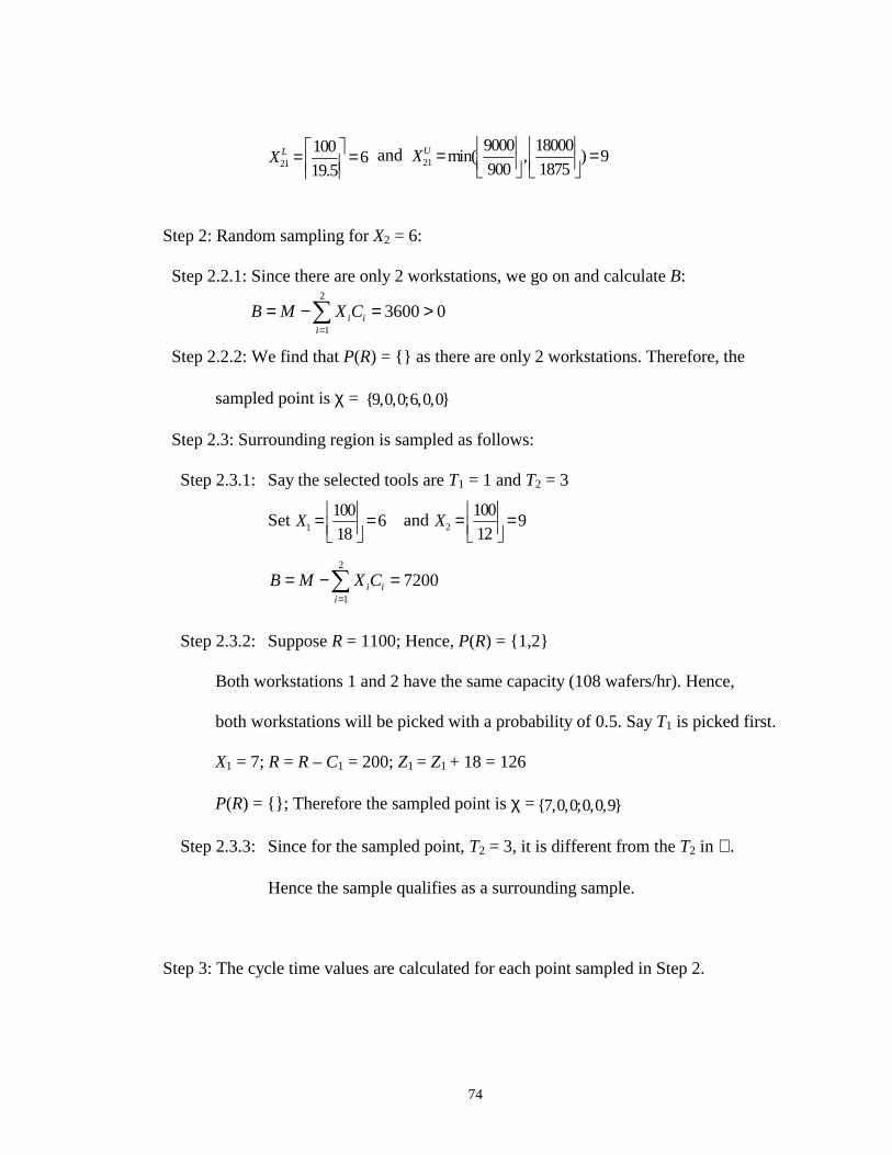
74

and

Step 2: Random sampling for X2 = 6:

Step 2.2.1: Since there are only 2 workstations, we go on and calculate B:

Step 2.2.2: We find that P(R) = {} as there are only 2 workstations. Therefore, the

sampled point is χ =

Step 2.3: Surrounding region is sampled as follows:

Step 2.3.1: Say the selected tools are T1 = 1 and T2 = 3

Set and

Step 2.3.2: Suppose R = 1100; Hence, P(R) = {1,2}

Both workstations 1 and 2 have the same capacity (108 wafers/hr). Hence,

both workstations will be picked with a probability of 0.5. Say T1 is picked first.

X1 = 7; R = R – C1 = 200; Z1 = Z1 + 18 = 126

P(R) = {}; Therefore the sampled point is χ =

Step 2.3.3: Since for the sampled point, T2 = 3, it is different from the T2 in ℑ .

Hence the sample qualifies as a surrounding sample.

Step 3: The cycle time values are calculated for each point sampled in Step 2.

21

1006

19.5LX

= = 21

9000 18000min( , ) 9

900 1875UX

= =

2

1

3600 0i ii

B M X C=

= − = >∑

{9,0,0;6,0,0}

1

1006

18X

= = 2

1009

12X

= =

2

1

7200i ii

B M X C=

= − =∑

{7,0,0;0,0,9}

75

Step 4: Let us say, the best sampled point (with least estimated cycle time value) is

found in the surrounding region: χ = . We find that

ℑ * = ≠ ℑ =

Therefore, after backtracking, we get ℑ + = and θ+= {}; the partition depth is now set

to 2, (the node type is primary now) and the procedure is repeated.

4.8 Description of the analytical algorithm

This algorithm deals with a solution space that consists of only one tool type per

workstation, as in NPA-II. Like NPAs, it does not build up on the low-cost, feasible

solution provided by the heuristic. We implemented two analytical algorithms and the

one that was chosen as the benchmark, is described below. The comparison of results for

the two analytical algorithms is given in the appendix.

4.8.1 Notation

The following notation is used in addition to that of the heuristic:

Ti selected tool type at workstation i

Xi number of tools for workstation i

Ti and Xi are the decision variables, whose properties Ci and µi can be defined as:

Ci = Cij if Ti = j;

µi = µij if Ti = j;

Zi capacity of the workstation i; (Zi = Xi*µi)

jth highest workstation capacity, amongst those under consideration

θ set of the values of the number of tools corresponding to Ti:

{0,15,0;10,0,0}.

11{ }T

11 23{ , }T T 11 21{ , }T T

1 2{ , ,..., }nX X X

jxZ

76

f(θc) cycle time evaluated using the analytical formula for M/M/m queues, at the

current iteration

f(θp) cycle time evaluated using the analytical formula for M/M/m queues, at the

previous iteration

χ

4.8.2 Description

Let Ti = j, such that µij > µik for all k ≤ zi and k ≠ j. If µij = µik, then choose the less

expensive tool type. Set Ci = Cij; µi = µij.

Step 1: Check feasibility

For i = 1,...,n:

Set

Set

If B < 0, then

Return the solution as infeasible (even though the heuristic solution

might be feasible for the problem instance)

Else

Perform Step 2

Step 2: Return the solution

Initialize f(θp) = ∞

111 12 1 1 2{ , ,..., ;......; , ,..., }nz n n nzX X X X X X

ii

Xλµ

=

1

n

i ii

B M X C=

= −∑

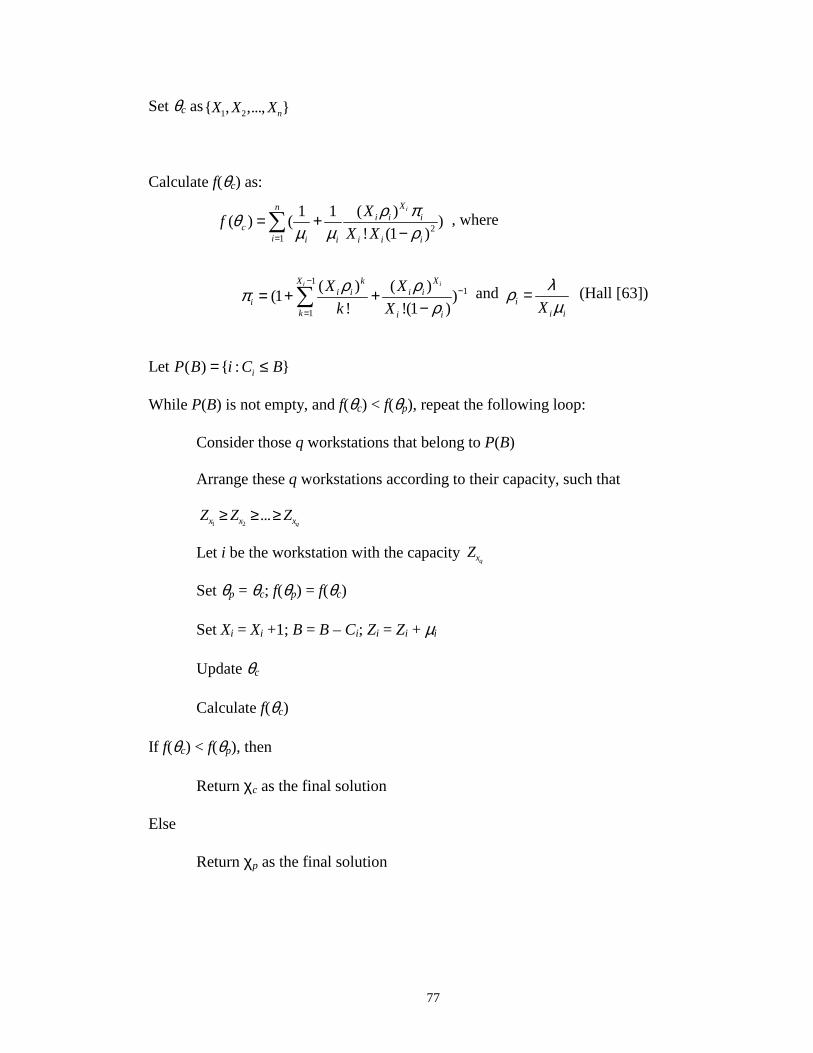
77

Set θc as

Calculate f(θc) as:

, where

and (Hall [63])

Let

While P(B) is not empty, and f(θc) < f(θp), repeat the following loop:

Consider those q workstations that belong to P(B)

Arrange these q workstations according to their capacity, such that

Let i be the workstation with the capacity

Set θp = θc; f(θp) = f(θc)

Set Xi = Xi +1; B = B – Ci; Zi = Zi + µi

Update θc

Calculate f(θc)

If f(θc) < f(θp), then

Return χc as the final solution

Else

Return χp as the final solution

( ) { : }iP B i C B= ≤

1 2...

qx x xZ Z Z≥ ≥ ≥

qxZ

1 2{ , ,..., }nX X X

21

( )1 1( ) ( )

! (1 )

iXni i i

ci i i i i i

Xf

X X

ρ πθµ µ ρ=

= +−∑

11

1

( ) ( )(1 )

! !(1 )

ii XX ki i i i

ik i i

X X

k X

ρ ρπρ

−−

=

= + +−∑ i

i iX

λρµ

=

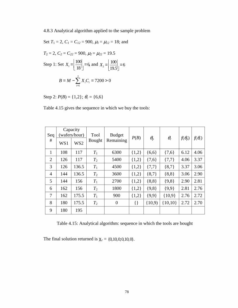
78

4.8.3 Analytical algorithm applied to the sample problem

Set T1 = 2, C1 = C12 = 900, µ1 = µ12 = 18; and

T2 = 2, C2 = C22 = 900, µ2 = µ22 = 19.5

Step 1: Set , and

Step 2: P(B) = {1,2}; θc = {6,6}

Table 4.15 gives the sequence in which we buy the tools:

Capacity (wafers/hour) Seq

# WS1 WS2

Tool Bought

Budget Remaining

P(B) θp θc f(θp) f(θc)

1 108 117 T1 6300 {1,2} {6,6} {7,6} 6.12 4.06

2 126 117 T2 5400 {1,2} {7,6} {7,7} 4.06 3.37

3 126 136.5 T1 4500 {1,2} {7,7} {8,7} 3.37 3.06

4 144 136.5 T2 3600 {1,2} {8,7} {8,8} 3.06 2.90

5 144 156 T1 2700 {1,2} {8,8} {9,8} 2.90 2.81

6 162 156 T2 1800 {1,2} {9,8} {9,9} 2.81 2.76

7 162 175.5 T1 900 {1,2} {9,9} {10,9} 2.76 2.72

8 180 175.5 T2 0 {} {10,9) {10,10} 2.72 2.70

9 180 195

The final solution returned is χc =

2

1

7200 0i ii

B M X C=

= − = >∑

1

1006

18X

= = 2

1006

19.5X

= =

{0,10,0;0,10,0}.

Table 4.15: Analytical algorithm: sequence in which the tools are bought

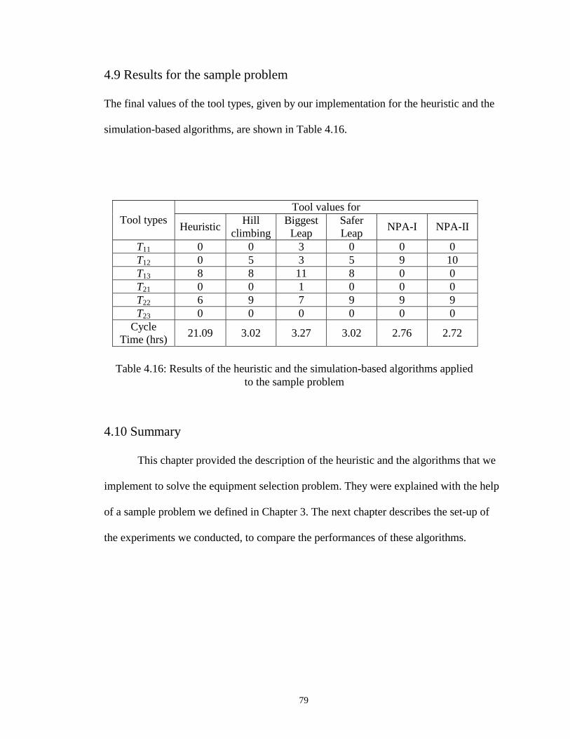
79

4.9 Results for the sample problem

The final values of the tool types, given by our implementation for the heuristic and the

simulation-based algorithms, are shown in Table 4.16.

Tool values for Tool types

Heuristic Hill

climbing Biggest

Leap Safer Leap

NPA-I NPA-II

T11 0 0 3 0 0 0 T12 0 5 3 5 9 10 T13 8 8 11 8 0 0 T21 0 0 1 0 0 0 T22 6 9 7 9 9 9 T23 0 0 0 0 0 0

Cycle Time (hrs)

21.09 3.02 3.27 3.02 2.76 2.72

4.10 Summary

This chapter provided the description of the heuristic and the algorithms that we

implement to solve the equipment selection problem. They were explained with the help

of a sample problem we defined in Chapter 3. The next chapter describes the set-up of

the experiments we conducted, to compare the performances of these algorithms.

Table 4.16: Results of the heuristic and the simulation-based algorithms applied to the sample problem

80

5. RESULTS AND DISCUSSION

This chapter reports and discusses the results that we obtained by conducting

experiments for the equipment selection problem, and compares the hill climbing,

biggest leap, safer leap and nested partitions algorithms against the analytical algorithm.

Section 5.1 describes the experimental set-up comprising the administrator, the problem

sets, the simulation model and the output metrics based on which we compare the

algorithms. Section 5.2 lists the results we obtained for the problem sets when the cost

and capacity are not correlated, and when they are correlated respectively. In Section

5.3, we summarize those results.

5.1 Experimental design

The administrator (designed in Delphi 5®1), the input template files (Microsoft

Excel®2), the simulation engine (Factory Explorer 2.5®3) along with the simulation

model file (Microsoft Excel) that it interacts with, and the output file (Microsoft Excel),

are the four components of the experimental architecture. The administrator controls all

other components. The purpose of these experiments is to compare the performance of

the algorithms over a range of problem sets and determine how the characteristics of the

problem instances affect the algorithms’ performance. The instances are not based on

any specific problems from industrial applications. The input template files contain the

input data for the simulation models. The administrator reads the input data from these

1 Registered trademark of Borland Software Corporation 2 Registered trademark of Microsoft Inc. 3 Registered trademark of Wright, Williams and Kelley Inc.

81

files and runs the heuristic to find the initial feasible solution. Then it populates the

simulation model file that the simulation engine interacts with and runs one of the search

algorithms under consideration. During the run, it updates the simulation model file,

executes the simulation engine and at the end of the search, records the output data in the

output file.

5.1.1 Input template files

There are two input template files, each containing a different problem set. Each

problem set contains 16 data sets with 10 data instances per data set. Hence there are a

total of 160 problem instances in one input template file. The difference between the two

problem sets is the correlation between the cost and capacity. Ideally, the cost of a tool

would increase with an increase in its capacity. In Problem Set 1, the cost and capacity

are not correlated, while in Problem Set 2, they are.

The input for the Problem Set 1 is as follows.

P = cost factor for tool types = $1000

λ = desired throughput = 100 wafers per hour

n = number of workstations = 5

r = expected number of tools per workstation = 2 or 10

zi = number of tool types per workstation = 2 or 5

α = lower bound of cost range = 0.5 or 0.8

β = multiplier for budget = 1 or 3

µij = capacity of the jth tool at the ith workstation

Cij = cost of the jth tool at the ith workstation

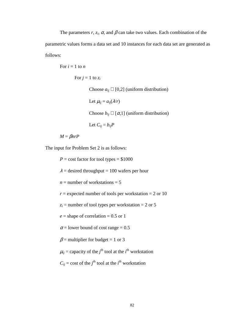
82

The parameters r, zi, α, and β can take two values. Each combination of the

parametric values forms a data set and 10 instances for each data set are generated as

follows:

For i = 1 to n

For j = 1 to zi

Choose aij ∈ [0,2] (uniform distribution)

Let µij = aij(λ/r)

Choose bij ∈ [α,1] (uniform distribution)

Let Cij = bijP

M = βnrP

The input for Problem Set 2 is as follows:

P = cost factor for tool types = $1000

λ = desired throughput = 100 wafers per hour

n = number of workstations = 5

r = expected number of tools per workstation = 2 or 10

zi = number of tool types per workstation = 2 or 5

e = shape of correlation = 0.5 or 1

α = lower bound of cost range = 0.5

β = multiplier for budget = 1 or 3

µij = capacity of the jth tool at the ith workstation

Cij = cost of the jth tool at the ith workstation

83

The parameters r, zi, e, and β can each take two values. Each combination of the

parametric values forms a data set and 10 instances for every data set are generated as

follows:

For i = 1 to n

For j = 1 to zi

Choose bij ∈ [α,1] (uniform distribution)

Let aij = 2(bij)e

Let µij = aij(λ/r)

Let Cij = bijP

M = βnrP

The link to the data sets can be found at the following website:

http://www.isr.umd.edu/Labs/CIM/projects/mfgsys/index.html

5.1.2 Simulation model

There is one product, Wafer, which enters the system as one lot of 25 wafers

every 0.25 hours. The lot inter-arrival times and the lot processing times are

exponentially distributed. The mean processing time on a tool of type j at workstation i

is 25/µij. The factory is a flow shop. Each lot must visit each workstation in the same

sequence. The number of lots that visit each tool type at a workstation is proportional to

the tool’s capacity. In other words, even if a high capacity tool is idle at a workstation,

the lot coming out of the queue might get routed to another idle tool at the same

workstation with a much lower capacity. It is assumed that there are no travel times for

the lots, from one workstation to the next. Therefore, the layout of the factory is not

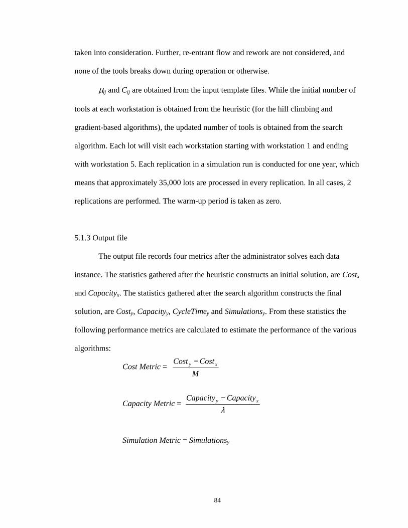
84

taken into consideration. Further, re-entrant flow and rework are not considered, and

none of the tools breaks down during operation or otherwise.

µij and Cij are obtained from the input template files. While the initial number of

tools at each workstation is obtained from the heuristic (for the hill climbing and

gradient-based algorithms), the updated number of tools is obtained from the search

algorithm. Each lot will visit each workstation starting with workstation 1 and ending

with workstation 5. Each replication in a simulation run is conducted for one year, which

means that approximately 35,000 lots are processed in every replication. In all cases, 2

replications are performed. The warm-up period is taken as zero.

5.1.3 Output file

The output file records four metrics after the administrator solves each data

instance. The statistics gathered after the heuristic constructs an initial solution, are Costx

and Capacityx. The statistics gathered after the search algorithm constructs the final

solution, are Costy, Capacityy, CycleTimey and Simulationsy. From these statistics the

following performance metrics are calculated to estimate the performance of the various

algorithms:

Cost Metric =

Capacity Metric =

Simulation Metric = Simulationsy

M

CostCost xy −

λxy CapacityCapacity −

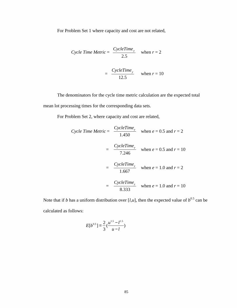
85

For Problem Set 1 where capacity and cost are not related,

Cycle Time Metric = when r = 2

= when r = 10

The denominators for the cycle time metric calculation are the expected total

mean lot processing times for the corresponding data sets.

For Problem Set 2, where capacity and cost are related,

Cycle Time Metric = 1.450

yCycleTime when e = 0.5 and r = 2

= 7.246

yCycleTime when e = 0.5 and r = 10

= 1.667

yCycleTime when e = 1.0 and r = 2

= 8.333

yCycleTime when e = 1.0 and r = 10

Note that if b has a uniform distribution over [l,u], then the expected value of b0.5 can be

calculated as follows:

1.5 1.50.5 2

[ ] ( )3

u lE b

u l

−=−

5.2yCycleTime

5.12yCycleTime

86

5.2 Results

The results for the output metrics for the algorithms we implemented are shown

in Tables 5.1 and 5.2, in subsections 5.2.1 and 5.2.2 respectively. Table 5.1 corresponds

to the case when the cost and capacity of the tools are not correlated. Table 5.2

corresponds to the case when the cost and capacity are correlated.

The nested partitions algorithm-I (NPA-I) was first applied to data set 16, for the

case when the cost and capacity are correlated. It was found that it required unreasonable

computational effort compared to the hill climbing and the gradient-based algorithms,

without producing much improvement in the output metrics. Hence, we discontinued its

application to the other data sets and developed another implementation of the nested

partitions algorithm, that we called NPA-II. Note that NPA-I and NPA-II were used only

once to solve each data instance.

The number of feasible data instances for a particular data set indicates the

number of data instances in that data set for which all the algorithms generated results.

The output metrics were averaged over the number of feasible data instances. All the

data instances for all data sets are found to be feasible when the cost and capacity are

correlated. However, it is not so in the other case. From the data instances that we

declared infeasible, the following deserve a special mention:

• 4th data instance in the 1st data set: only NPA-II generated a solution

• 4th data instance in the 9th data set: only the hill climbing and the gradient-based

algorithms generated a solution

• 1st and 6th data instances in the 11th data set: only the hill climbing, gradient-based

and analytical algorithms generated a solution

87

5.2.1 Cost and capacity are not correlated

Based on Table 5.1, we plotted the results for the output metrics for all the

algorithms, which we discuss next.

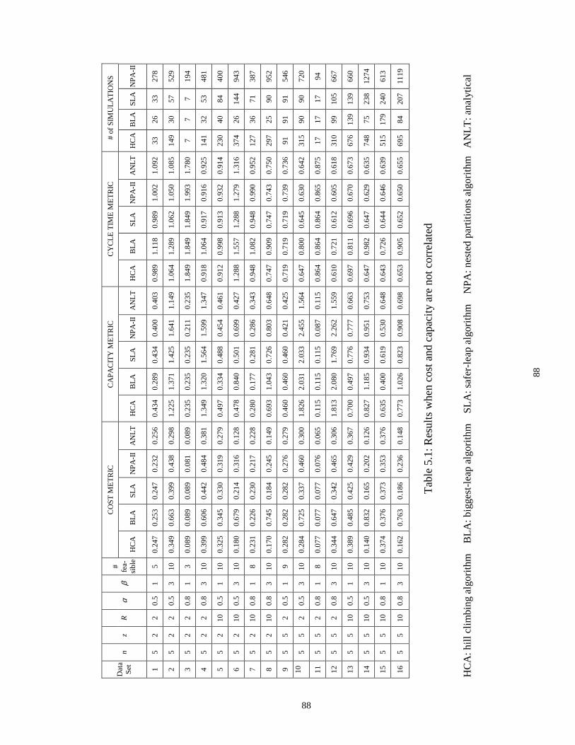
88

CO

ST M

ET

RIC

C

APA

CIT

Y M

ET

RIC

C

YC

LE

TIM

E M

ET

RIC

#

of S

IMU

LA

TIO

NS

Dat

a Se

t n

z R

α

β #

fe

a-si

ble

HC

A

BL

A

SLA

N

PA-I

I A

NL

T

HC

A

BL

A

SLA

N

PA-I

I A

NL

T

HC

A

BL

A

SLA

N

PA-I

I A

NL

T

HC

A

BL

A

SLA

N

PA-I

I

1 5

2 2

0.5

1 5

0.24

7 0.

253

0.24

7 0.

232

0.25

6 0.

434

0.28

9 0.

434

0.40

0 0.

403

0.98

9 1.

118

0.98

9 1.

002

1.09

2 33

26

33

27

8

2 5

2 2

0.5

3 10

0.

349

0.66

3 0.

399

0.43

8 0.

298

1.22

5 1.

371

1.42

5 1.

641

1.14

9 1.

064

1.28

9 1.

062

1.05

0 1.

085

149

30

57

529

3 5

2 2

0.8

1 3

0.08

9 0.

089

0.08

9 0.

081

0.08

9 0.

235

0.23

5 0.

235

0.21

1 0.

235

1.84

9 1.

849

1.84

9 1.

993

1.78

0 7

7 7

194

4 5

2 2

0.8

3 10

0.

399

0.60

6 0.

442

0.48

4 0.

381

1.34

9 1.

320

1.56

4 1.

599

1.34

7 0.

918

1.06

4 0.

917

0.91

6 0.

925

141

32

53

481

5 5

2 10

0.

5 1

10

0.32

5 0.

345

0.33

0 0.

319

0.27

9 0.

497

0.33

4 0.

488

0.45

4 0.

461

0.91

2 0.

998

0.91

3 0.

932

0.91

4 23

0 40

84

40

0

6 5

2 10

0.

5 3

10

0.18

0 0.

679

0.21

4 0.

316

0.12

8 0.

478

0.84

0 0.

501

0.69

9 0.

427

1.28

8 1.

557

1.28

8 1.

279

1.31

6 37

4 26

14

4 94

3

7 5

2 10

0.

8 1

8 0.

231

0.22

6 0.

230

0.21

7 0.

228

0.28

0 0.

177

0.28

1 0.

286

0.34

3 0.

948

1.08

2 0.

948

0.99

0 0.

952

127

36

71

387

8 5

2 10

0.

8 3

10

0.17

0 0.

745

0.18

4 0.

245

0.14

9 0.

693

1.04

3 0.

726

0.80

3 0.

648

0.74

7 0.

909

0.74

7 0.

743

0.75

0 29

7 25

90

95

2

9 5

5 2

0.5

1 9

0.28

2 0.

282

0.28

2 0.

276

0.27

9 0.

460

0.46

0 0.

460

0.42

1 0.

425

0.71

9 0.

719

0.71

9 0.

739

0.73

6 91

91

91

54

6

10

5 5

2 0.

5 3

10

0.28

4 0.

725

0.33

7 0.

460

0.30

0 1.

826

2.03

1 2.

033

2.45

5 1.

564

0.64

7 0.

800

0.64

5 0.

630

0.64

2 31

5 90

90

72

0

11

5 5

2 0.

8 1

8 0.

077

0.07

7 0.

077

0.07

6 0.

065

0.11

5 0.

115

0.11

5 0.

087

0.11

5 0.

864

0.86

4 0.

864

0.86

5 0.

875

17

17

17

94

12

5 5

2 0.

8 3

10

0.34

4 0.

647

0.34

2 0.

465

0.30

6 1.

813

2.08

0 1.

769

2.26

2 1.

559

0.61

0 0.

721

0.61

2 0.

605

0.61

8 31

0 99

10

5 66

7

13

5 5

10

0.5

1 10

0.

389

0.48

5 0.

425

0.42

9 0.

367

0.70

0 0.

497

0.77

6 0.

777

0.66

3 0.

697

0.81

1 0.

696

0.67

0 0.

673

676

139

139

660

14

5 5

10

0.5

3 10

0.

140

0.83

2 0.

165

0.20

2 0.

126

0.82

7 1.

185

0.93

4 0.

951

0.75

3 0.

647

0.98

2 0.

647

0.62

9 0.

635

748

75

238

1274

15

5 5

10

0.8

1 10

0.

374

0.37

6 0.

373

0.35

3 0.

376

0.63

5 0.

400

0.61

9 0.

530

0.64

8 0.

643

0.72

6 0.

644

0.64

6 0.

639

515

179

240

613

16

5 5

10

0.8

3 10

0.

162

0.76

3 0.

186

0.23

6 0.

148

0.77

3 1.

026

0.82

3 0.

908

0.69

8 0.

653

0.90

5 0.

652

0.65

0 0.

655

695

84

207

1119

HC

A: h

ill c

lim

bing

alg

orit

hm

BL

A: b

igge

st-l

eap

algo

rith

m

SL

A: s

afer

-lea

p al

gori

thm

N

PA: n

este

d pa

rtit

ions

alg

orit

hm

AN

LT

: ana

lyti

cal

Tab

le 5

.1: R

esul

ts w

hen

cost

and

cap

acit

y ar

e no

t cor

rela

ted

88

89

Figure 5.1 shows the comparison of the cost metric. When the budget is low (β =

1), we find that for data sets 3 and 11 (α = 0.8), the cost metric for all algorithms is very

low. For these data sets, the cost of each tool is very high. Hence, the heuristic itself

requires a major chunk of the budget, not leaving enough money for further purchase of

tools. The argument is also supported by the fact that the number of feasible instances

for these data sets is 3 and 8 respectively. The cost metric for data sets 13 and 15 (z = 5)

is very high. With a large number of tools available at each workstation for these data

sets, and no correlation between the cost and capacity, it is more likely that a high

capacity tool is available at a low price. Hence at the end of the heuristic, more money is

available for further purchase. At low budget, it can be seen that on an average all the

algorithms behave in a similar manner, except for the biggest leap algorithm (BLA) that

spends more money after the heuristic due to its inherent greedy nature.

When the budget is high (β = 3), we find that the trend for BLA is opposite to

that for the other algorithms. For data sets 6, 8, 14 and 16 (r = 10), the budget available

is the highest. Hence at each iteration, BLA spends a lot of money buying tools with low

capacities too, and runs out of the available budget with further improvement in the

cycle time still possible. When the available budget is low, as for the other data sets, it is

not able to spend as much and hence the cost metric is low. The other algorithms

however, are most likely to buy only tools having the highest capacity and hence do not

end up spending the whole budget available, whenever possible. Since the cost metric is

inherently normalized with respect to the total budget available, it is lower when r = 10

compared to when r = 2. This is because when r = 10, the capacity of the tools is very

low and a lot of tools are purchased. But after a certain stage, it does not help in reducing

90

the cycle time. In other words, the addition of a fast tool to a few similar fast tools will

have more impact on the cycle time compared to the addition of a slow tool to a lot of

similar slow tools. Hence, even though the capacity is 80% smaller when r = 10, it does

not imply that 5 times the money should be spent in further purchasing the tools, as there

will be no reduction in the cycle time after a certain stage. We shall refer to this logic as

quick sand reasoning. The hill climbing algorithm (HCA) performs closest to the

analytical algorithm (ANLT), whose cost metric turns out to be the lowest amongst all

the algorithms. The cost metric for the safer leap algorithm (SLA) is slightly higher than

that for HCA, but lower than that for the nested partitions algorithm-II (NPA-II).

It can also be seen that the cost metric for data sets 6, 8, 14 and 16 (β = 3, r = 10)

is lower for all algorithms except BLA, than that for data sets 5, 7, 13 and 15 (β = 1, r =

10) respectively. The reason is the high budget with respect to which the metric is

normalized. The increase in the cost metric from data set 7 to 8, and the approximate

equality for data sets 5 and 6 for NPA-II are exceptions.

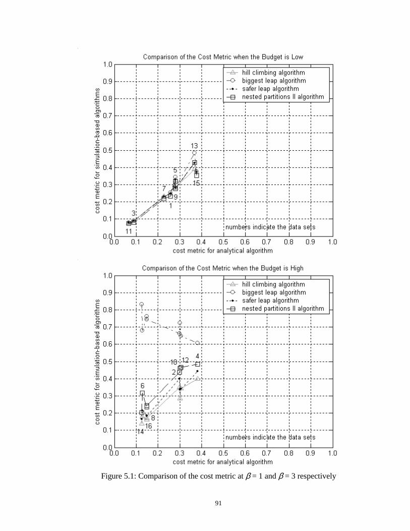
91

Figure 5.1: Comparison of the cost metric at β = 1 and β = 3 respectively

92

Figure 5.2 shows the comparison of the capacity metric. When the budget is low

(β = 1), we find that for data sets 3 and 11, the capacity metric for all the algorithms is

very low. For these data sets, the cost metric is low too. Since not enough money was

available to purchase the tools after the heuristic, the system could not gain much

capacity. On a similar basis, the high values of the capacity metric for data sets 13 and

15 can be explained, where the cost metric was high as well. When the available budget

is low, and only one tool is bought at each iteration for BLA, the behavior of HCA, BLA

and SLA is the same. When the available budget is high, BLA tends to increase the

capacity of the workstations in a highly skewed manner, so that the overall capacity of

the system remains low, as can be seen from the Figure 5.2. All other algorithms

perform more or less in a similar manner, except for data sets 13 and 15. For data set 13,

the capacity metric for SLA and NPA-II is higher than that for the other algorithms. For

these algorithms the cost metric is higher too, for the corresponding data set. However

for data set 15, even though the cost metric was approximately the same, the capacity

metric of NPA-II is low. This implies a skewed distribution of capacity amongst the

workstations.

When the budget is high (β = 3), it is seen that for all algorithms, the capacity

metric for data sets 6, 8, 14 and 16 (r = 10) is lower than that for data sets 2, 4, 10 and 12

(r = 2) respectively. This is due to quick sand reasoning. It is interesting to note that

BLA has a higher capacity metric, yet a lower cost metric when r = 2, compared to when

r = 10. This is because when r = 2, the capacity of each tool is high, but the available

budget is low. Hence, the whole budget is not squandered in a skewed manner, as is the

tendency of BLA. ANLT has the lowest capacity metric. HCA performs closest to

93

ANLT, barring data sets 10 and 12. The capacity metric is highest for BLA when r = 10

and for NPA-II when r = 2. The behavior of SLA is similar to that of HCA only when r

= 10.

It can also be seen that the magnitude of increase in the capacity metric from data

sets 5, 7, 13 and 15 (β = 1, r = 10), to data sets 6, 8, 14 and 16 (β = 3, r = 10)

respectively, is lower than that for the corresponding data sets when r = 2, for all the

algorithms except BLA. This is due to quick sand reasoning.

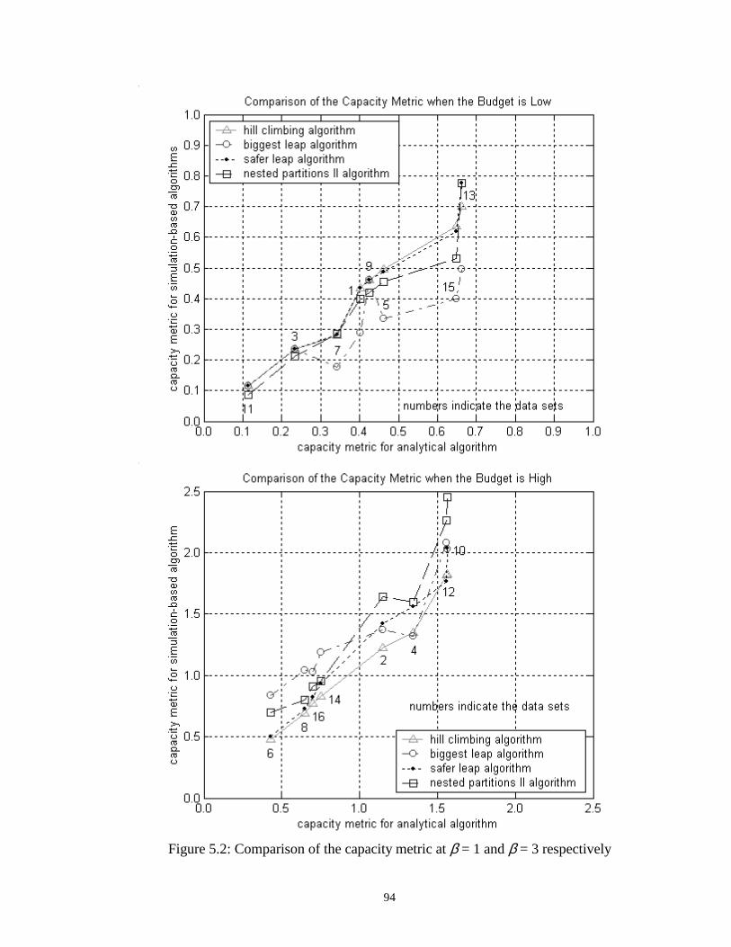
94

Figure 5.2: Comparison of the capacity metric at β = 1 and β = 3 respectively

95

Figure 5.3 shows the comparison of the cycle time metric. When the budget is

low (β = 1), we find that for data sets 9, 13 and 15, the cycle time metric is low. The

capacity metric for these data sets is high too. Although capacity metric for data set 3 is

higher than that for 11, the cycle time metric indicates otherwise. Out of the eight

feasible instances that were taken into consideration for data set 11, two had no addition

to capacity after the heuristic and two others had insignificant addition to the capacity.

For data set 3, only three instances were feasible. Hence the data was insufficient for

concrete comparison, as it resulted in skewed metrics. The performance of all algorithms

except BLA appears to be similar for the cycle time metric. For BLA, it is always higher

than the rest, when it is not equal to that for HCA and SLA.

When the budget is high (β = 3), we notice that the cycle time metric for data sets

10, 12, 14 and 16 (z = 5) is lower as compared to others (z = 2). For data sets 10 and 12,

the capacity metric was highest too. For data sets 14 and 16, a greater choice of tools at a

workstation implies greater probability for at least one tool to have a very high capacity.

This translates as a lower cycle time value, and hence as a lower cycle time metric

despite the capacity metric not being among the highest. The performance of all the

algorithms but BLA matches closely. The cycle time metric for BLA is always higher,

despite a higher capacity metric for a few data sets. This is due to the purchase of low

capacity tools. Wafer lots at these low capacity tools would take more time to get

processed. It is unlikely however, for the other algorithms to buy tools that would not

have the highest capacity at a workstation.

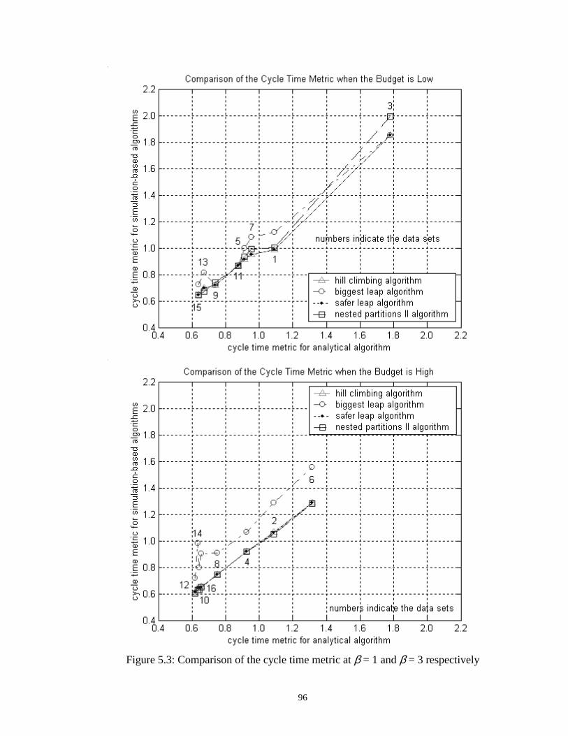
96

Figure 5.3: Comparison of the cycle time metric at β = 1 and β = 3 respectively

97

Figure 5.4 shows the comparison of the simulation metric. When the budget is

low (β = 1), we find that the number of simulations for data sets 1, 3, 9 and 11 (r = 2) is

equal and very small for HCA, BLA and SLA. This is due to less money available at the

end of the heuristic to purchase more tools. For NPA-II however, the number of

simulations is higher due to the search process, as it has no initial solution to work with.

For data sets 13 and 15 (r = 10, z = 5), since the available budget is high and there are

many tool types with low capacity (compared to when r = 2) to choose from, the number

of simulations is higher for HCA. For NPA-II also, the number of primary and

secondary nodes is more when z = 5, resulting in a higher simulation metric. BLA and

SLA have the lowest values for the simulation metric.

When the budget is high (β = 3), we find that the number of simulations for data

sets 2 and 4 (r = 2, z = 2) is small. This is due to less money being available (compared

to when r = 10) and few tool types to choose from. For similar reasons, data sets 14 and

16 (r = 10, z = 5) have the highest simulation metric. It is seen that NPA-II requires a lot

of simulation runs compared to the other algorithms. This is because when the budget

available is high, NPA-II has a broader width to cover at each depth level for the

secondary nodes. BLA and SLA require fewer simulation runs compared to HCA.

98

Figure 5.4: Comparison of the simulation metric at β = 1 and β = 3 respectively

99

Figures 5.5 and 5.6 give an idea about how effectively the budget that is spent,

reduces the cycle time. A higher capacity to cost ratio implies that the system gained

more capacity by spending the same amount of money. A high ratio along with a low

cycle time metric provides an ideal combination. Figure 5.5 shows the comparison when

the budget is low (β = 1). HCA performs the best for data sets 1 and 9 (r = 2, α = 0.5),

and relatively well for data sets 3, 5 and 13 and 15. BLA performs well only when the

available budget is very low, so that its behavior tends to that of HCA. This can be seen

for data sets 3 and 9. For data sets 5, 7, 13 and 15 (r = 10), it performs the worst. SLA’s

performance is always very close to that of HCA. NPA-II performs the best for data set

13 and relatively well for all other data sets except for 11 (r = 2, α = 0.8) where it

performs the worst. It has a tendency to spend a little more money for the same amount

of capacity, achieving almost the same reduction in the cycle time. ANLT performs the

best for data sets 3, 5, 7, 11 and 15, and relatively well for 9 and 13.

Figure 5.6 shows the comparison when the budget is high (β = 3). HCA performs

relatively well, while BLA performs the worst for all data sets. SLA’s performance is

close to that of HCA, although it spends more money for the same capacity. NPA-II and

ANLT also perform relatively well for all the data sets. NPA-II, again has a tendency to

spend more money for the same capacity, though it achieves the minimum cycle time for

all data sets.

100

Figure 5.5: Comparison of cycle time metric vs. the ratio of capacity and cost metrics at

β = 1

101

Figure 5.6: Comparison of cycle time metric vs. the ratio of capacity and cost metrics at

β = 3

102

5.2.2 Cost and capacity are correlated

Based on Table 5.2, we plotted the results for the output metrics for all the

algorithms, which we discuss next.

10

3

CO

ST M

ET

RIC

C

APA

CIT

Y M

ET

RIC

C

YC

LE

TIM

E M

ET

RIC

#

of S

IMU

LA

TIO

NS

Dat

a Se

t n

Z

r e

β # fea-

sibl

e H

CA

B

LA

SL

A

NPA

-II

AN

LT

H

CA

B

LA

SL

A

NPA

-II

AN

LT

H

CA

B

LA

SL

A

NPA

-II

AN

LT

H

CA

B

LA

SL

A

NPA

-II

1 5

2 2

0.5

1 10

0.

307

0.30

7 0.

307

0.31

7 0.

313

0.39

9 0.

399

0.39

9 0.

492

0.39

3 1.

207

1.20

7 1.

207

1.17

7 1.

190

38

38

38

428

2 5

2 2

0.5

3 10

0.

288

0.66

6 0.

312

0.50

0 0.

355

1.69

8 2.

920

1.92

3 2.

626

1.73

9 1.

023

1.01

7 1.

023

0.95

5 0.

966

116

21

37

630

3 5

2 2

1.0

1 10

0.

227

0.21

7 0.

228

0.21

5 0.

214

0.52

3 0.

457

0.52

3 0.

552

0.51

3 1.

279

1.35

9 1.

279

1.25

0 1.

247

29

22

29

540

4 5

2 2

1.0

3 10

0.

321

0.70

0 0.

398

0.50

6 0.

316

1.78

9 2.

181

2.09

1 2.

660

1.68

5 0.

947

0.99

5 0.

945

0.89

7 0.

915

125

28

50

613

5 5

2 10

0.

5 1

10

0.47

1 0.

563

0.50

7 0.

509

0.46

2 0.

976

0.49

9 1.

070

0.90

5 0.

863

1.02

0 1.

091

1.09

1 0.

958

0.96

1 30

0 39

90

64

1

6 5

2 10

0.

5 3

10

0.16

1 0.

846

0.19

1 0.

225

0.15

7 0.

981

1.44

5 1.

184

1.02

5 0.

844

1.01

0 1.

012

1.00

8 0.

942

0.94

8 29

7 28

90

11

96

7 5

2 10

1.

0 1

10

0.44

6 0.

451

0.44

6 0.

415

0.41

2 0.

802

0.47

3 0.

818

0.76

5 0.

793

0.96

9 1.

040

0.97

1 0.

922

0.92

3 27

3 37

89

64

8

8 5

2 10

1.

0 3

10

0.16

1 0.

815

0.18

5 0.

203

0.13

6 0.

871

1.15

5 0.

972

0.98

3 0.

791

1.00

1 1.

053

0.99

9 0.

937

0.94

4 30

8 28

95

83

2

9 5

5 2

0.5

1 10

0.

393

0.39

3 0.

393

0.38

8 0.

376

0.40

9 0.

409

0.40

9 0.

558

0.42

7 1.

217

1.21

7 1.

217

1.14

8 1.

207

107

107

107

684

10

5 5

2 0.

5 3

10

0.35

1 0.

682

0.43

2 0.

549

0.40

5 1.

874

3.47

2 2.

360

2.64

3 1.

744

1.01

4 1.

018

1.00

5 0.

910

0.92

4 32

5 64

12

6 71

6

11

5 5

2 1.

0 1

10

0.21

7 0.

217

0.21

7 0.

205

0.19

4 0.

409

0.40

6 0.

406

0.49

8 0.

485

1.24

7 1.

247

1.24

7 1.

133

1.14

9 55

55

55

75

1

12

5 5

2 1.

0 3

10

0.37

2 0.

709

0.41

7 0.

472

0.37

1 2.

181

2.03

9 2.

517

2.43

0 2.

076

0.90

6 0.

944

0.90

4 0.

827

0.83

6 33

8 13

2 15

2 70

7

13

5 5

10

0.5

1 10

0.

580

0.58

2 0.

580

0.53

2 0.

539

1.08

2 0.

613

1.08

1 0.

784

0.86

9 1.

003

1.09

7 1.

004

0.91

0 0.

908

820

156

416

719

14

5 5

10

0.5

3 10

0.

214

0.85

6 0.

262

0.26

6 0.

178

1.22

6 2.

036

1.53

5 1.

137

0.87

4 1.

002

1.01

5 0.

999

0.90

9 0.

916

950

94

290

1153

15

5 5

10

1.0

1 10

0.

448

0.44

7 0.

449

0.42

3 0.

434

0.74

6 0.

564

0.75

8 0.

757

0.84

9 0.

916

0.99

8 0.

916

0.82

6 0.

824

618

160

360

780

16

5 5

10

1.0

3 10

0.

201

0.80

4 0.

242

0.24

5/

0.14

5 0.

952

1.79

8 1.

193

1.12

3/

0.82

5 0.

926

1.03

3 0.

928

0.83

5/

0.84

2 88

3 90

28

6 11

60/

0.31

8*

0.75

2*

0.86

4*

2771

*

HC

A: h

ill c

lim

bing

alg

orit

hm

BL

A: b

igge

st-l

eap

algo

rith

m

SL

A: s

afer

-lea

p al

gori

thm

N

PA: n

este

d pa

rtit

ions

alg

orit

hm

AN

LT

: ana

lyti

cal

*

indi

cate

s th

e re

sult

s fo

r N

PA-I

. Not

e th

at th

is a

lgor

ithm

was

app

lied

onl

y to

one

dat

a se

t.

Tab

le 5

.2: R

esul

ts w

hen

cost

and

cap

acit

y ar

e co

rrel

ated

103

Figure 5.7 shows the comparison of the cost metric. When the budget is low (β =

1), we find that for data sets 3 and 11 (r = 2, e = 1.0), the cost metric is very low. This is

because the available budget is very low, and compared to data sets 1 and 9 (r = 2, e =

0.5), the capacity of the tools is lower. Hence the heuristic itself eats up a major chunk of

the budget, not leaving enough money to purchase more tools. We also notice that the

cost metric for data sets 5 and 13 (r = 10, e = 0.5) is very high. The capacity of the tools

is higher compared to data sets 7 and 15 (r = 10, e = 1.0) and hence the heuristic does

not spend much money, thereby leaving a huge sum to be spent to purchase more tools.

For data sets 1, 3, 9 and 11 (r = 2) the performance of all the algorithms is nearly the

same. For the others however, the cost metric for ANLT and NPA-II is generally lower.

Barring data set 5 where BLA has the highest cost metric, HCA, SLA and BLA behave

in a similar manner.

When the budget is high (β = 3), we find that the trend for BLA is opposite to

that for the other algorithms, as in the first problem set. It has the highest cost metric for

all data sets. For data sets 6, 8, 14 and 16 (r = 10), the cost metric is very low compared

to other data sets where r = 2. This is due to the huge budget available, with respect to

which the metric is normalized, and quick sand reasoning. BLA, unlike the other

algorithms, ends up spending the whole budget. HCA has the lowest cost metric for data

sets 2 and 10 (r = 2, e = 0.5) and ANLT for the rest. The nested paritions-I (NPA-I)

algorithm has a very high cost metric for data set 16, but it is still lower than that for

BLA. SLA performs worse than HCA, but better than NPA-II, whose cost metric is

generally high, and especially when r = 2.

104

105

It can also be seen that the cost metric for data sets 6, 8, 14 and 16 (β = 3, r =

10), is lower for all algorithms except BLA, than that for 5, 7, 13 and 15 (β = 1, r = 10),

respectively. The reason is the high budget with respect to which the metric is

normalized and quick sand reasoning.

106

Figure 5.7: Comparison of the cost metric at β = 1 and β = 3 respectively

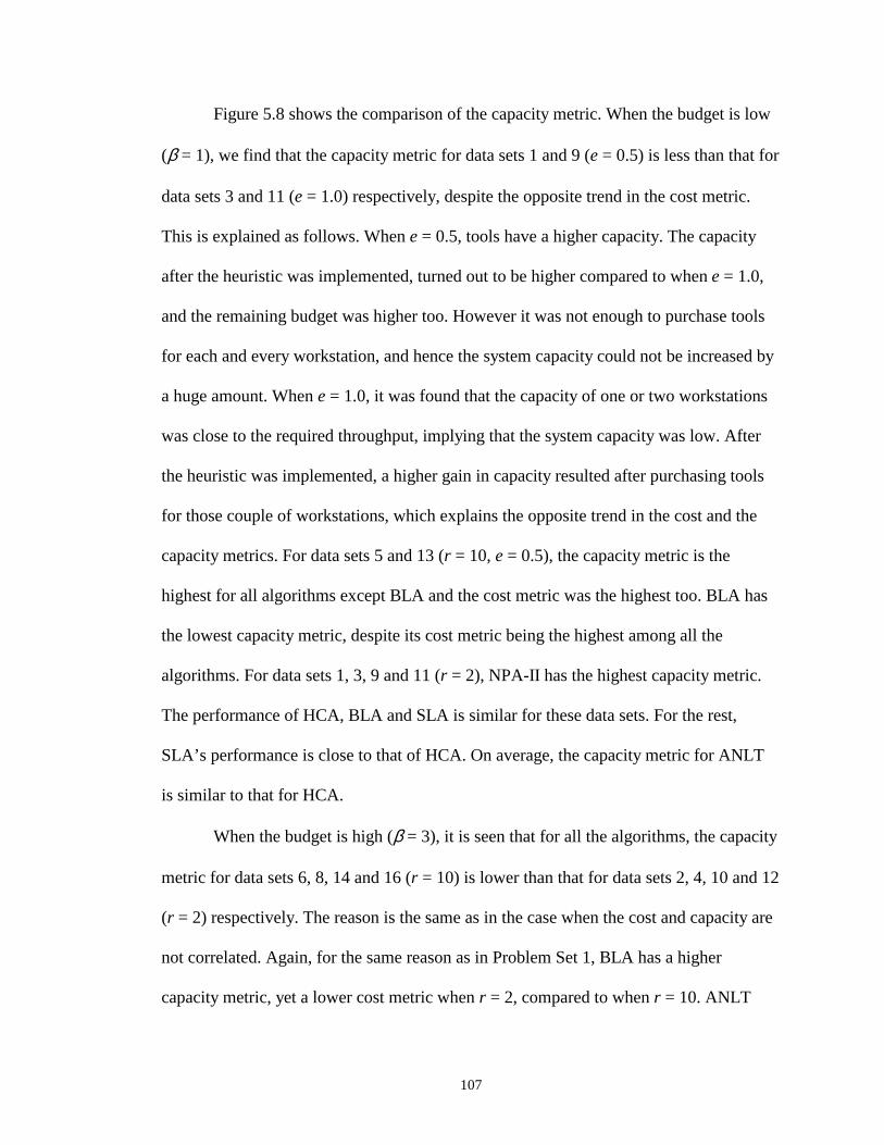
107

Figure 5.8 shows the comparison of the capacity metric. When the budget is low

(β = 1), we find that the capacity metric for data sets 1 and 9 (e = 0.5) is less than that for

data sets 3 and 11 (e = 1.0) respectively, despite the opposite trend in the cost metric.

This is explained as follows. When e = 0.5, tools have a higher capacity. The capacity

after the heuristic was implemented, turned out to be higher compared to when e = 1.0,

and the remaining budget was higher too. However it was not enough to purchase tools

for each and every workstation, and hence the system capacity could not be increased by

a huge amount. When e = 1.0, it was found that the capacity of one or two workstations

was close to the required throughput, implying that the system capacity was low. After

the heuristic was implemented, a higher gain in capacity resulted after purchasing tools

for those couple of workstations, which explains the opposite trend in the cost and the

capacity metrics. For data sets 5 and 13 (r = 10, e = 0.5), the capacity metric is the

highest for all algorithms except BLA and the cost metric was the highest too. BLA has

the lowest capacity metric, despite its cost metric being the highest among all the

algorithms. For data sets 1, 3, 9 and 11 (r = 2), NPA-II has the highest capacity metric.

The performance of HCA, BLA and SLA is similar for these data sets. For the rest,

SLA’s performance is close to that of HCA. On average, the capacity metric for ANLT

is similar to that for HCA.

When the budget is high (β = 3), it is seen that for all the algorithms, the capacity

metric for data sets 6, 8, 14 and 16 (r = 10) is lower than that for data sets 2, 4, 10 and 12

(r = 2) respectively. The reason is the same as in the case when the cost and capacity are

not correlated. Again, for the same reason as in Problem Set 1, BLA has a higher

capacity metric, yet a lower cost metric when r = 2, compared to when r = 10. ANLT

108

has the lowest capacity metric for most data sets. HCA performs closest to ANLT,

barring data set 14. The capacity metric is highest for BLA when r = 10 and for data sets

2 and 10 (r = 2, e = 0.5). NPA-II has the highest capacity metric for data sets 4 and 12 (r

= 2, e = 1.0). The capacity metric for SLA is always higher than that for HCA. For data

set 16, NPA-I has the lowest capacity metric even though its cost metric is very high.

It can also be seen that the magnitude of increase in the capacity metric from data

sets 5, 7, 13 and 15 (β = 1, r = 10), to data sets 6, 8, 14 and 16 (β = 3, r = 10)

respectively, is lower than that for the corresponding data sets when r = 2, for all the

algorithms except BLA. This is due to the fact that the capacity of each tool is much

higher when r = 2, compared to when r = 10, and that the amount of money spent to gain

further capacity will not be proportional to the ratio between these two values of r, as

there will be no reduction in the cycle time on addition of a quick sand tool to a lot of

similar quick sand tools after a certain stage, as explained earlier.

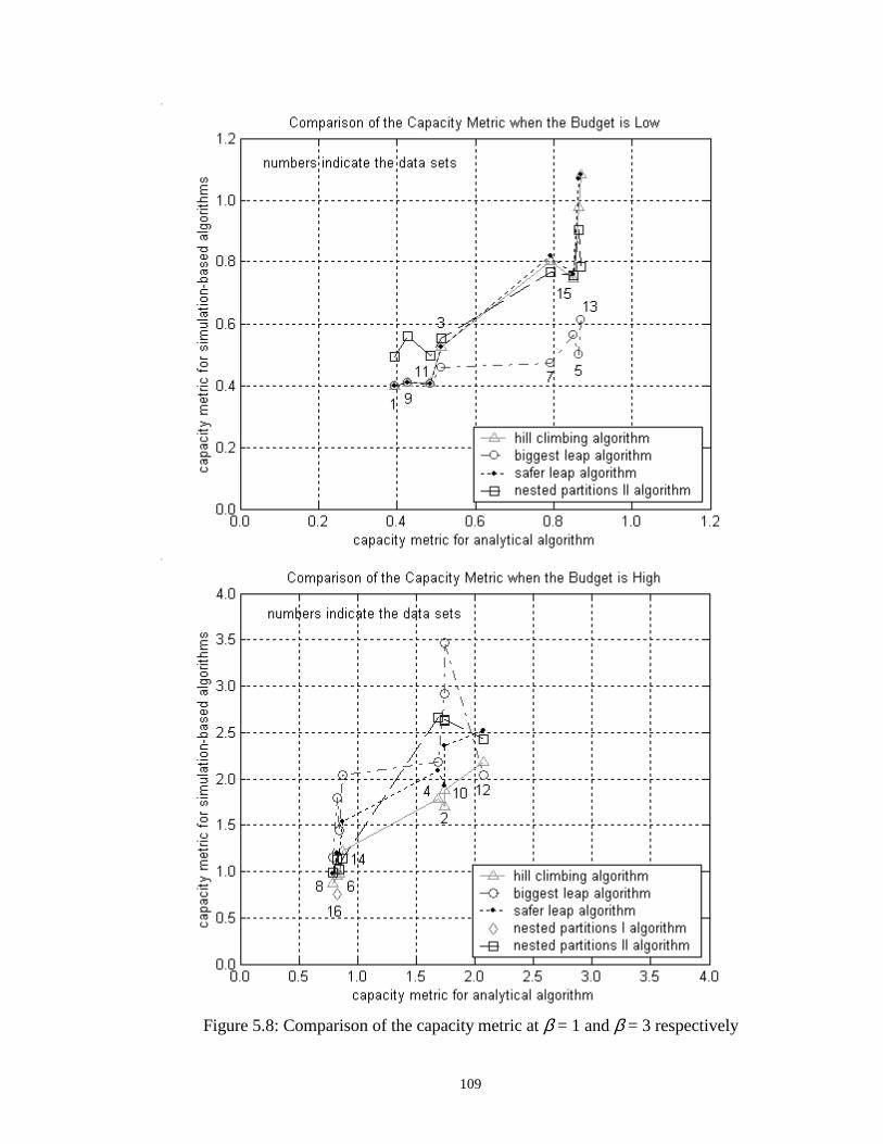
109

Figure 5.8: Comparison of the capacity metric at β = 1 and β = 3 respectively

110

Figure 5.9 shows the comparison of the cycle time metric. When the budget is

low (β = 1), we find that for data sets 5, 7, 13 and 15 (r = 10), the cycle time metric is

low. The capacity metric for these data sets is high too. Although data sets 3 and 11 (r =

2, e = 1.0) have a higher capacity metric than data sets 1 and 9 (r = 2, e = 0.5), it does

not translate into a lower cycle time. The reason is that when the budget available is low,

and e = 1.0, the capacity of tools is not as high compared to when e = 0.5. Hence the

heuristic spends a lot more money comparatively, and buys the tool with the highest

capacity to cost ratio, even though that capacity might be much below that of the highest

capacity tool at that workstation. After the heuristic is implemented, not enough money

is left to purchase the highest capacity tools. Hence the cycle time metric is high. The

performance of NPA-II and ANLT is approximately the same, and they have the lowest

cycle time metric. When r = 2, HCA, BLA and SLA perform similarly, and have the

highest cycle time metric. However when r = 10, BLA has the highest cycle time metric,

while the performance of SLA is close to that of HCA.

When the budget is high (β = 3), we notice that the cycle time metric for data set

12 is minimum. For this data set, the capacity metric was the highest. For data sets 6, 8,

14 and 16 (r = 10), the capacity metric is low. For these data sets with 16 being an

exception, the cycle time metric is among the highest. But surprisingly for 16 (r = 10), it

is among the lowest. NPA-II and ANLT have the lowest cycle time metric, while BLA

has the highest. The performance of SLA is almost similar to that of HCA. NPA-I has a

low cycle time metric too, but it is higher than that for NPA-II.

111

Figure 5.9: Comparison of the cycle time metric at β = 1 and β = 3 respectively

112

Figure 5.10 shows the comparison of the simulation metric. We find the analysis

exactly similar to that for the case when the cost and capacity are not correlated. When

the budget is low (β = 1), we find that the number of simulations for data sets 1, 3, 9 and

11 (r = 2) is equal, and very small for HCA, BLA and SLA. This is due to less money

being available at the end of the heuristic, to purchase more tools. For NPA-II however,

the number of simulations is higher due to the search process, as it has no initial solution

to work with. For data sets 13 and 15 (r = 10, z = 5), since the available budget is high

and there are many tool types with low capacity (compared to when r = 2) to choose

from, the number of simulations is higher for HCA. For NPA-II also, the number of

primary and secondary nodes is more when z = 5, resulting in a higher simulation metric.

BLA and SLA have the lowest values for the simulation metric.

When the budget is high (β = 3), we find that the number of simulations for data

sets 2 and 4 (r = 2, z = 2) is small. This is due to less money being available (compared

to when r = 10) and few tool types to choose from. For similar reasons, data sets 14 and

16 (r = 10, z = 5) have the highest simulation metric. It is seen that NPA-II requires a lot

of simulation runs compared to the other algorithms. BLA and SLA require much less

simulation runs compared to HCA. For data set 16, NPA-I requires a prohibitive amount

of simulation effort.

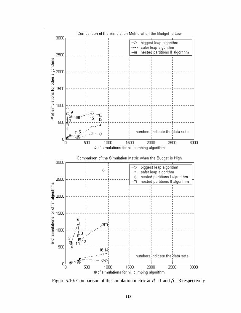
113

Figure 5.10: Comparison of the simulation metric at β = 1 and β = 3 respectively

114

Figures 5.11 and 5.12 show the comparison between the cycle time metric and

the ratio of the capacity to cost metrics. Figure 5.11 shows the comparison when the

budget is low (β = 1). NPA-II performs the best for data sets 1, 3 and 9 (r = 2) and

relatively well for data sets 7, 11 and 15. ANLT performs the best for data sets 7 and 15

(r = 10, e = 1.0), and relatively well for data set 11. Performance of HCA and SLA is

similar, and relatively good for data sets 5, 7 and 13 (r = 10). BLA performs the worst.

Figure 5.12 shows the comparison when the budget is high (β = 3). HCA

performs relatively well, while BLA performs the worst for all the data sets. SLA’s

performance is close to that of HCA. NPA-II has the lowest cycle time metric but

generally spends more money for the same capacity. ANLT performs relatively well for

data sets 4, 8, 12 and 16 (e = 1.0). For data set 16, NPA-I spends relatively much more

for the same amount of capacity, yet does not have the lowest cycle time metric.

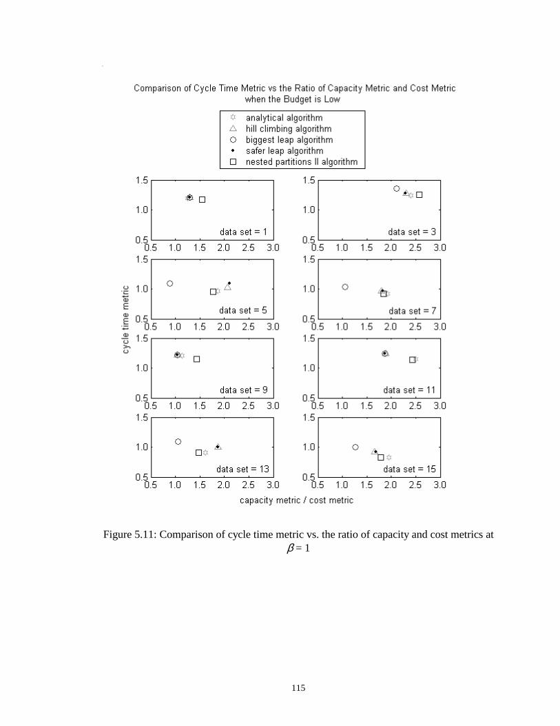
115

Figure 5.11: Comparison of cycle time metric vs. the ratio of capacity and cost metrics at

β = 1

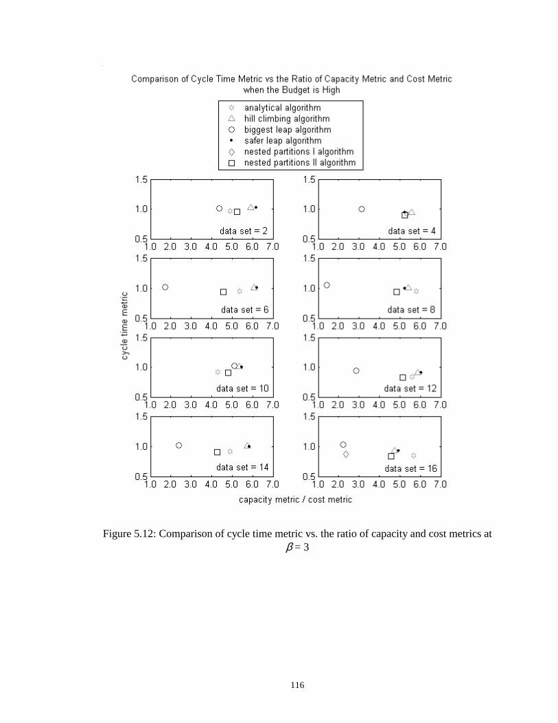
116

Figure 5.12: Comparison of cycle time metric vs. the ratio of capacity and cost metrics at

β = 3

117

5.2.3 Comparison between Problem Sets 1 and 2

It is found that the cost and capacity metrics are higher, when the cost and

capacity are correlated (Problem Set 2), compared to when they are not (Problem Set 1).

This is because the average capacity of a tool is higher in Problem Set 2, and since the

cost and capacity are correlated, we end up spending more money. The cycle time metric

for Problem Set 2 though, is higher than that for Problem Set 1. This can be explained as

follows. The cycle time metric is normalized with respect to the average total processing

time. Hence a higher value for the metric for a particular data instance would imply a

longer waiting time. Since the search algorithms continue buying tools even though there

would be only a small improvement in the cycle time, the average total waiting time in

the queue is very less at the end, compared to the average total processing time. Hence,

as a fraction of the total processing time, the waiting time will be more when the total

processing time is less, which corresponds to the case when the average capacity of tools

is higher, as in Problem Set 2. The simulation metric is also higher for Problem Set 2.

For HCA, BLA and SLA, there will be more iterations in the search process when the

capacity of the tools is higher. This is because addition of a higher capacity tool would

be more likely to improve the cycle time, than the addition of a lower capacity tool. For

NPA-II, the range of tool values over which the partitioning is done for a secondary

node, will be higher when the cost and capacity are correlated. Section 4.7.2 in Chapter 4

provides the description on partitioning the nodes for NPA-II. The upper bound for the

tool value is inversely proportional to the sum of the ratios of the cost to the capacity of

the tools chosen, which will be higher for Problem Set 1. Hence there will be fewer total

simulation runs for the secondary nodes when the cost and capacity are not correlated.

118

5.3 Summary of the results

Based on the results and explanations, we summarize as follows. The

performance of the algorithms was compared through cost, capacity, cycle time and

simulation metrics. A higher cost metric implies that a greater portion of the budget was

spent in purchasing the tools. A higher capacity metric implies a greater capacity in the

system. A higher cycle time metric implies that a wafer lot spends a longer time in the

system. A higher simulation metric implies that a large number of simulation runs are

needed to reach the final solution.

HCA and ANLT tend to have the lowest cost metric, followed by SLA, NPA-II

and NPA-I respectively. BLA has the highest cost metric.

HCA and ANLT have a relatively high capacity metric when the budget is low,

but have a very low capacity metric at high values of budget. BLA has the lowest

capacity metric at low values of budget and the highest capacity metric at high values of

budget. At high values of budget, SLA has a higher capacity metric compared to HCA.

NPA-I has the lowest capacity metric. NPA-II in general, has a high capacity metric.

ANLT and NPA-II almost always have the lowest cycle time metric, followed by

HCA and SLA that have similar values of the cycle time metric. NPA-I performs slightly

better than HCA and SLA. BLA almost always has the highest cycle time metric.

BLA has the lowest simulation metric, followed by SLA. HCA requires more

simulation runs than SLA, but fewer than NPA-II. NPA-I requires an exorbitant amount

of simulation effort.

119

Table 5.3 summarizes the performance of the algorithms with respect to the

output metrics. The number of stars reflects the relative performance of each algorithm

on that metric.

Algorithm Cost Capacity Cycle Time Simulation HCA * * * * * * * * * * * * * * BLA * * * * * * * * * * SLA * * * * * * * * * * * * * * *

NPA-I * * * * * * * * NPA-II * * * * * * * * * * * * * * * ANLT * * * * * * * * * * * * * -

* worst performance * * * * * best performance

5.4 Summary

This chapter discussed the experimental set-up and the results that we obtained.

Each of the six algorithms was used to find solutions to the 320 instances of the problem.

After describing the results in detail, this chapter summarized the results and discussed

the performance of the algorithms on each metric. The next chapter summarizes the

conclusions and lists the limitations, contributions and the future work.

Table 5.3: Performance of the algorithms under consideration

120

6. SUMMARY AND CONCLUSIONS

This chapter summarizes the research work that we performed and draws the

conclusions. Section 6.1 discusses the suitability of the algorithms that we implemented,

with respect to the special structure of the equipment selection problem. Section 6.2 lists

the contributions of our research. Section 6.3 mentions some of the limitations of our

implementation. Finally, in Section 6.4 we discuss the future work.

6.1 Conclusions

An equipment selection problem was formulated with minimization of the

average cycle time as the objective, along with constraints on the budget and minimum

throughput on the system. We developed and implemented five simulation-based

algorithms, namely hill climbing, biggest leap, safer leap, nested partitions-I and nested

partitions-II, and an analytical algorithm for the problem. After testing them on two

different problem sets characterized by the presence or absence of a correlation between

the cost and capacity of tools, we found that there are trade-offs associated with the

performance of the simulation-based algorithms. The hill climbing algorithm spends the

least amount of money to achieve a very low cycle time but requires a large amount of

simulation effort. The biggest leap algorithm spends an unreasonable amount of money

and yet is not able to reduce the cycle time appreciably. The quality of solutions is the

worst, but the simulation effort required is the least. The safer leap algorithm

incorporates the best features of the hill climbing and the biggest leap algorithms,

providing good quality solutions with reasonable simulation effort. NPA-II requires a

121

tremendous amount of simulation effort, but provides good quality solutions, although at

a slightly higher cost. NPA-I requires the most amount of simulation effort, but spends a

lot of money to achieve a low cycle time value. It performs better than the biggest leap

algorithm, but is dominated by NPA-II. The analytical algorithm turns out to be the best

amongst all, as it spends the least amount of money to achieve a very low cycle time

without any simulation effort at all. This benchmark algorithm was chosen after

implementing and comparing two searches (described in the appendix) over a wide

range of problem instances.

It is worth noting that the equipment selection problem we considered has a

special structure to it. It seems intuitive that given a choice between a variety of tools,

the addition of a higher capacity tool will serve to reduce the cycle time more. Moreover,

a proportionate distribution of the capacity of workstations tends to avoid serious

bottlenecks that occur when the capacity distribution is skewed. Although the hill

climbing algorithm (explained in Chapter 4, Section 4.3) invariably selects the tool with

the highest capacity at the end of each iteration, it does so without making use of any

knowledge about the problem structure. The biggest leap algorithm (explained in

Chapter 4, Section 4.4) tends to select the tool with the highest capacity, though it ends

up buying the other tools with lower capacity at that workstation as well. It is oblivious

of the problem structure too. The safer leap algorithm (explained in Chapter 4, Section

4.5) exploits the problem structure, as it buys tools with the highest capacity for at least

one workstation at the end of each iteration, thereby trying to increase the capacity of all

the workstations uniformly. NPA-I (explained in Chapter 4, Section 4.6) also tries to buy

tools with the highest capacity, although, due to its random search, it also buys tools

122

with lower capacities. The modifications made to develop NPA-II (explained in Chapter

4, Section 4.7) not only reduce the simulation runs involved but also direct the efforts of

the algorithm towards selecting the highest capacity tool to help it utilize the special

structure of the problem that NPA-I did not. The analytical algorithm (explained in

Chapter 4, Section 4.8) we presented is completely based on the special structure that the

equipment selection problem has. However, it may be inappropriate for more complex

manufacturing systems such as job shops where different workstations have different

throughput requirements. If the interarrival and processing times have other probability

distributions, a more general GI/G/m approximation would be required to estimate

manufacturing cycle times. See Herrmann and Chincholkar [64] for instance.

Therefore, when selecting a simulation-based stochastic algorithm for any given

problem, it is beneficial to have prior knowledge about any special properties that might

be inherent in the structure of the problem. This helps to fine tune the algorithm to direct

the search for the optimum solution in the most efficient manner.

6.2 Contributions

We presented five simulation-based algorithms and two analytical searches to

solve the equipment selection problem. Unlike other manufacturing system design

problems, this novel formulation requires selection amongst various tool types at a given

workstation. Combining the cycle time objective with a budget constraint is another

unique feature that addresses the trade-off between initial investment and system

performance. The hill climbing algorithm was based on the generalized hill climbing

algorithm described by Sullivan and Jacobson [1]. The biggest leap algorithm was based

123

on the gradient-based method described by Mellacheruvu [62]. We designed the new

safer leap algorithm by combining the salient features of the hill climbing and the

biggest leap algorithms. The nested partitions algorithm proposed by Shi and Olafsson

[3], formed the basis for our novel implementation of NPA-I and NPA-II.

When a manufacturing system incorporating complexities such as break down of

tools, maintenance schedules or re-entrant flows is to be designed, it is difficult to

develop analytical algorithms to solve an associated optimization problem. Sometimes, a

rough estimate is needed to get a quick idea about what the optimal solution might look

like, and on other occasions, an accurate solution might be required, which may take

time. We discussed the performance of the algorithms we implemented for our problem,

with respect to such trade-offs between the quality of solution and the time and effort

involved. No systematic comparison of these algorithms has been done before.

We also showed the importance of the knowledge of the problem structure,

through the implementation of the safer leap algorithm, two different versions of the

nested partitions algorithm, and the analytical algorithm. In general, the black box

approach that assumes no knowledge about the system that is being simulated performs

well for problems that do not reveal much information about their structure. However,

those methods that utilize the knowledge of the problem structure, whenever such

information is available, dominate the black box approach. In Chapter 2, we mentioned

the research work, such as that of Gong, Ho and Zhai [47], pertaining to the simulation-

based algorithms that utilize the special structure of the problem under consideration.

We also referred to the research that has been conducted to compare the performance of

variants of a particular algorithm on a specific problem, such as that by Alrefaei and

124

Andradottir [43]. Similar to the literature related to the combination of salient features of

two or more algorithms, such as that by Shi, Olafsson and Chen [51], our safer leap

algorithm combines the salient features of the hill climbing algorithm and the biggest

leap algorithm, which by themselves, do not utilize the special problem structure of our

equipment selection problem. NPA-II exploits the structure better by purchasing only

one tool type per workstation. Further, its implementation suggests a greater probability

of selecting the tool type with the highest capacity. Compared to the simulation-based

algorithms, the analytical algorithm that is completely based on utilizing the special

problem structure provides the best results at no simulation cost. Our research work

therefore, emphasizes the importance of the knowledge of the problem structure as well

as the algorithms, so as to enable a customized implementation of the algorithms

utilizing the special properties that the problem might have.

6.3 Limitations

We made a few basic assumptions for our simulation model. These were

described in Section 5.1.2 of Chapter 5. Ours was a simple manufacturing system,

without any tool breakdowns, multiple product flows, rework, maintenance or re-entrant

flow. Improvement in cycle time of a magnitude greater than or equal to 0.01 hours

(precision of Factory Explorer 2.5) was accepted as sufficient reason to purchase another

tool, if the budget permitted so. The same value of 0.01 hours was also used for the

analytical algorithms, as the lowest acceptable improvement in the cycle time. The

simulation model also assumed that the number of wafer lots that visit each tool type at a

workstation is proportional to the tool’s capacity.

125

Although in literature, the nested partitions algorithm has been combined with a

technique called optimal computing budget allocation (OCBA) to ensure a larger

allocation of simulation effort amongst the potentially good designs, we did not

implement OCBA. Further, the selection of the number of samples for the partitioned

and the surrounding regions did not have any strong basis due to lack of any concrete

guidelines.

6.4 Future work

The scope of the problem we considered could be extended to sharing equipment

between workstations, which is common in practical situations with re-entrant flow.

Further complexities could be modeled in the form of breakdown of tools, maintenance

schedules and multiple product families.

For the hill climbing, biggest leap and safer leap algorithms, a better heuristic

could be employed to obtain a different starting point for these search algorithms.

Techniques to help the nested partitions algorithm focus on potentially good

configurations and reduce the simulation effort involved could also be employed.

Another approach would be to add the cost of equipment purchase with economic

measures related to cycle time such as the cost of holding work-in-process, to determine

the system design that minimizes the system life cycle costs.

Finally, we could study the performance of the analytical algorithm on systems

with more general probability distributions for processing time and inter-arrival time.

126

APPENDIX

This appendix presents the two analytical algorithms that were considered to

decide the benchmark-algorithm for the simulation-based algorithms and discusses the

experimental results.

1. Description of the algorithms

The algorithms search a solution space that consists of only one tool type per

workstation.

1.1 Notation

The notation used is as follows:

λ desired throughput

M budget available

n number of workstations

zi total number of different tool types at workstation i; i = 1, ..., n

Tij tool of type j at workstation i; j = 1, ..., zi

µij capacity of Tij tool

Cij cost of Tij tool

Uij capacity per unit cost of Tij tool =

k iteration number

greatest integer less than or equal to x

smallest integer greater than or equal to x

Ti selected tool type at workstation i

Xi number of tools for workstation i

x

x

ij

ijC

µ

127

Ti and Xi are the decision variables. If Ti = j, Ci = Cij and µi = µij.

θ the number of tools: {X1, X2, …, Xn}

f(θk) the manufacturing cycle time of the system given a solution θk

χ {X11, X12, …, X1,z1; …; Xn1, Xn2, …, Xn,zn

}

1.2 Description

The two search algorithms are called Algorithm I (A-I) and Algorithm II (A-II).

The only difference in the algorithms is the selection of Ti.

For Algorithm I (A-I), let Ti = j, such that µij > µik for all k ≤ zi and k ≠ j. If µij =

µik, then choose the tool type with lower cost. Set Ci = Cij; µi = µij.

For Algorithm II (A-II), let Ti = j, such that Uij > Uik for all k ≤ zi and k ≠ j. If Uij

= Uik, then choose the tool type with higher capacity. Set Ci = Cij; µi = µij.

After Ti are selected, each algorithm proceeds as follows:

Step 1: Check feasibility

For i = 1, ..., n:

Set

Set

If B < 0, then

Return the solution as infeasible

Else

Initialize k = 0

ii

Xλµ

=

1

n

i ii

B M X C=

= −∑

128

θk = {X1, X2, …, Xn}

For i = 1, ..., n,

i

i iX

λρµ

=

11

1

( ) ( )(1 )

! !(1 )

ii XX li i i i

il i i

X X

l X

ρ ρπρ

−−

=

= + +−∑

2

1

( )1 1( ) ( )

! (1 )

iXni i i

ki i i i i i

Xf

X X

ρ πθµ µ ρ=

= +−∑

Output CostI = X1C1 + … + XnCn and Cycle TimeI = f(θk)

Step 2: Perform the search

Let f(θk-1) = ∞.

Let ε be a small positive number (in our experiments, ε = 0.01 hours).

Define P(B) = {i: Ci ≤ B} as the set of workstations with “affordable” tools (that is, the

cost of a tool at any of these workstations is not greater than the unspent budget).

While P(B) is not empty and f(θk) ≤ f(θk-1) - ε, repeat the following loop:

Let i be the workstation in P(B) that currently has the least capacity (the smallest

value of Xiµi).

Update Xi, B, and k as follows: Xi = Xi +1; B = B – Ci; k = k + 1

θk = {X1, X2, …, Xn}

Calculate f(θk)

Update P(B)

If f(θk) > f(θk-1) - ε, then revise Xi, B, and k as follows: Xi = Xi - 1; B = B + Ci; k = k - 1

Construct the solution χ from θk as follows:

129

For all i and j, Xij = Xi if Ti = j, and 0 otherwise

Output CostF = X1C1 + … + XnCn and Cycle TimeF = f(θk)

2. Experiments

The algorithms were run on the Problem Set 2 described in Section 5.1.1 of

Chapter 5. Each search algorithm (A-I and A-II) was run on each instance. The output

of each run included five performance measures. The performance measures of the

initial solution are CostI and Cycle TimeI. The performance measures of the final

solution are CostF and Cycle TimeF. Since each data set is different, we normalized

these statistics by comparing the cost performance to the total budget for that data set

and comparing the cycle time performance to the expected total processing time of that

data set. If b has a uniform distribution over [l,u], then the expected value of b0.5 can be

calculated as follows:

1.5 1.50.5 2

[ ] ( )3

u lE b

u l

−=−

From these statistics, the following performance metrics are calculated to

estimate the performance of each algorithm on each instance:

Cost MetricI = CostI/M. Cost MetricF = CostF/M.

Cycle Time MetricI = Cycle TimeI/1.450 and Cycle Time MetricF = Cycle TimeF/1.450

if e = 0.5 and r = 2 (Data sets 1, 2, 9, and 10).

Cycle Time MetricI = Cycle TimeI/7.246 and Cycle Time MetricF = Cycle TimeF/7.246

if e = 0.5 and r = 10 (Data sets 5, 6, 13, and 14).

Cycle Time MetricI = Cycle TimeI/1.667 and Cycle Time MetricF = Cycle TimeF/1.667

if e = 1.0 and r = 2 (Data sets 3, 4, 11, and 12).

130

Cycle Time MetricI = Cycle TimeI/8.333 and Cycle Time MetricF = Cycle TimeF/8.333

if e = 1.0 and r = 10 (Data sets 7, 8, 15, and 16).

The fifth performance measure was the number of iterations that the algorithm

performed before stopping. All of the metrics were averaged over all ten problem

instances. Table 1 shows the results for each algorithm on each data set. Figures 1 and 2

also display the cost and cycle time metrics. A larger cost metric implies that more of

the budget was spent purchasing tools. A larger cycle time metric implies that jobs spent

more time in the system.

3. Results

The last two columns in Table A1 show that the number of iterations for both

algorithms is approximately the same in most data sets. A-II does require more

iterations in some data sets. The most significant increases occur in data sets 9 and 11

because A-I selects, in general, more expensive tools and spends the budget more

quickly than A-II.

As shown in Table A1 and Figures A1 and A2, A-I constructs initial solutions

that have, in general, a larger cost metric and a smaller cycle time metric than the initial

solutions that A-II constructs. This results from A-I’s selection of large capacity tools,

which are expensive. But the initial solution is likely to have more than enough

capacity, which reduces congestion and cycle time. A-II selects, in general, smaller

tools, so the capacity of the initial solution will exceed the throughput constraint by a

smaller margin. Higher utilization will lead to larger cycle times.

131

At the end of the search, A-I finds solutions that have a larger cost metric than

the final solutions that A-II finds, but the performance on the cycle time metric is very

close. Compared to the initial solutions, the final solutions found have much larger cost

metrics and much smaller cycle time metrics. Thus, it is clear that the search algorithms

are useful for finding feasible, high-quality solutions.

Algorithm A-I was selected as the benchmark-algorithm based on its lower cycle

time values compared to A-II, for all the 16 data sets.

0

0.2

0.4

0.6

0.8

1

1.2

1 3 5 7 9 11 13 15 2 4 6 8 10 12 14 16

Data Set

Ave

rag

e C

ost

Met

ric

A-I Initial A-I Final A-II Initial A-II Final

Figure A1: Average cost metric

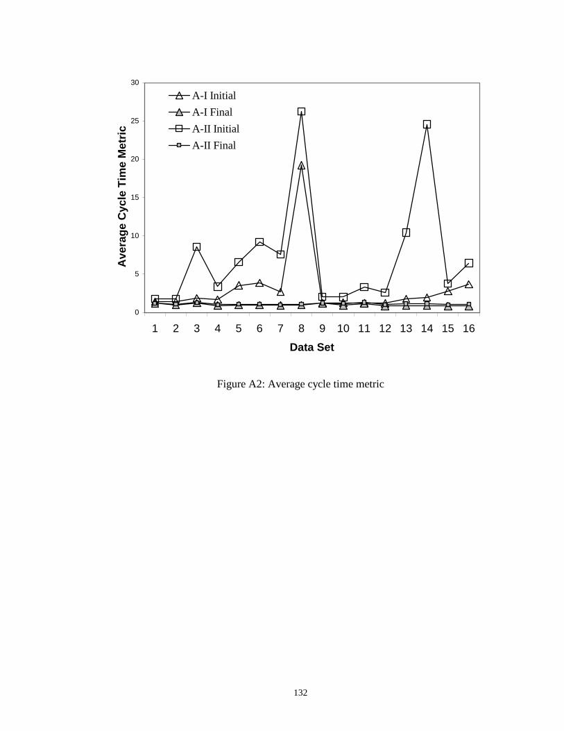
132

0

5

10

15

20

25

30

1 2 3 4 5 6 7 8 9 10 11 12 13 14 15 16

Data Set

Ave

rag

e C

ycle

Tim

e M

etri

c

A-I Initial

A-I Final

A-II Initial

A-II Final

Figure A2: Average cycle time metric

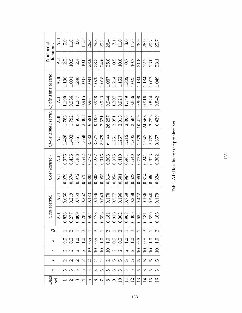
13

3

Cos

t Met

ric I

C

ost M

etri

c F

Cyc

le T

ime

Met

ric I

Cyc

le T

ime

Met

ric F

N

umbe

r of

It

erat

ions

D

ata

set

n z

r e

β A

-I

A-I

I A

-I

A-I

I A

-I

A-I

I A

-I

A-I

I A

-I

A-I

I 1

5 2

2 0.

5 1

0.82

3 0.

666

0.97

9 0.

976

1.42

0 1.

783

1.19

0 1.

196

2.3

5.0

2 5

2 2

0.5

3 0.

277

0.21

9 0.

574

0.45

6 1.

403

1.79

2 0.

966

1.09

1 10

.9

11.0

3

5 2

2 1.

0 1

0.80

9 0.

759

0.97

2 0.

988

1.86

1 8.

565

1.24

7 1.

298

2.4

3.6

4 5

2 2

1.0

3 0.

285

0.26

2 0.

578

0.54

2 1.

668

3.36

8 0.

915

1.00

7 10

.6

11.2

5

5 2

10

0.5

1 0.

504

0.43

3 0.

895

0.77

2 3.

532

6.58

1 0.

961

1.08

4 23

.9

26.3

6

5 2

10

0.5

3 0.

173

0.14

6 0.

303

0.25

7 3.

877

9.19

0 0.

948

1.07

9 23

.2

25.5

7

5 2

10

1.0

1 0.

553

0.54

3 0.

955

0.91

6 2.

679

7.57

1 0.

923

1.01

8 24

.6

25.2

8

5 2

10

1.0

3 0.

181

0.17

8 0.

314

0.30

3 19

.244

26

.257

0.

944

1.06

7 25

.0

26.4

9

5 5

2 0.

5 1

0.91

6 0.

577

0.95

4 0.

975

1.25

1 2.

051

1.20

7 1.

214

0.5

7.1

10

5 5

2 0.

5 3

0.30

2 0.

196

0.60

1 0.

410

1.26

7 2.

015

0.92

4 1.

152

10.0

11

.0

11

5 5

2 1.

0 1

0.90

8 0.

769

0.96

4 0.

961

1.21

5 3.

306

1.14

9 1.

309

0.7

3.0

12

5 5

2 1.

0 3

0.30

5 0.

258

0.62

9 0.

540

1.20

5 2.

584

0.83

6 1.

025

10.7

11

.6

13

5 5

10

0.5

1 0.

552

0.41

2 0.

951

0.72

8 1.

779

10.4

19

0.90

8 1.

134

21.8

26

.9

14

5 5

10

0.5

3 0.

181

0.13

6 0.

314

0.24

1 1.

947

24.5

65

0.91

6 1.

134

22.2

26

.9

15

5 5

10

1.0

1 0.

559

0.54

6 0.

980

0.92

3 2.

775

3.75

3 0.

824

1.01

3 23

.0

25.2

16

5

5 10

1.

0 3

0.18

6 0.

179

0.32

4 0.

302

3.66

7 6.

429

0.84

2 1.

049

23.1

25

.7

T

able

A1:

Res

ults

for

the

prob

lem

set

133

134

BIBLIOGRAPHY

[1] Sullivan, K.A. and S.H.Jacobson, "Ordinal hill climbing algorithms for discrete

manufacturing process design optimization problems," Journal of Discrete Event

Dynamic Systems: Theory and Applications, Vol.10, pp.307-324, 2000.

[2] Kiefer, J. and J.Wolfowitz, “Stochastic estimation of the maximum of a regression

function,” Annals of Mathematical Statistics, Vol.23, pp.462-466, 1952.

[3] Shi L. and S.Olafsson, "Nested partitions method for global optimization,"

Operations Research, Vol.48, No.3, pp.390-407, 2000.

[4] Bretthauer, K.M., "Capacity planning in manufacturing and computer networks,"

European Journal of Operational Research, Vol.91, pp.386-394, 1996.

[5] Swaminathan, J.M., "Tool capacity planning for semiconductor fabrication

facilities under demand uncertainty," European Journal of Operational Research,

Vol.120, pp.545-558, 2000.

[6] Swaminathan, J.M., "Tool procurement planning for wafer fabrication facilities: a

scenario based approach," IIE Transactions, Vol.34, No.2, pp.145-155, 2002.

[7] Connors, D.P., G.E.Feigin and D.D.Yao, "A queueing network model for

semiconductor manufacturing," IEEE Transasctions on Semiconductor

Manufacturing, Vol.9, No.3, pp.412-427, 1996.

[8] Bulgak, A.A. and J.L.Sanders, "Integrating a modified simulated annealing

algorithm with the simulation of a manufacturing system to optimize buffer sizes in

automatic assembly systems," Proceedings of the 1988 Winter Simulation

Conference, pp.684-690, 1988.

135

[9] Haddock, J. and J.Mittenthal, "Simulation optimization using simulated annealing,"

Computers and Industrial Engineering, Vol.22, No.4, pp.387-395, 1992.

[10] Ho, Y.-C., R.S.Sreenivas and P.Vakili, "Ordinal optimization of DEDS," Journal of

Discrete Event Dynamic Systems, Vol.2, pp.61-68, 1992.

[11] Choon, H.N., "Combining simulation with optimization search techniques for the

design of flexible manufacturing system," Proceedings of the International

Conference on Computer Integrated Manufacturing, pp.159-162, 1991.

[12] Cassandras, C.G. and C.G.Panayiotou, "Ordinal optimization for a class of

deterministic and stochastic discrete resource allocation problems," IEEE

Transactions on Automatic Control, Vol.43, No.7, pp.881-900, 1998.

[13] Lin, X., "Optimizing large complex systems by simulation - a practical approach,"

Proceedings of SPIE, Vol.3696, pp.192-201, 1999.

[14] Cassandras, C.G. and K.Gokbayrak, "Modeling and simulation-based solutions for

complex resource allocation problems," Proceedings of SPIE, Vol.3696, pp.160-

170, 1999.

[15] Hillier, F.S. and K.C.So, "On the simultaneous optimization of server and work

allocations in production line systems with variable processing times," Operations

Research, Vol.44, No.3, pp.435-443, 1996.

[16] Andradottir, S. and H.Ayhan, "Server assignment policies for maximizing the

steady-state throughput of finite queueing systems," Management Science, Vol.47,

No.10, pp.1421-1439, 2001.

[17] Palmeri, V. and D.W.Collins, "An analysis of the "K-step ahead" minimum

inventory variability policy® using SEMATECH semiconductor manufacturing

136

data in a discrete-event simulation model," Proceedings of the 6th IEEE

International Conference on Emerging Technologies and Factory Automation,

pp.520-527, 1997.

[18] Dumbrava, S., "The design of flexible manufacturing systems using simulations,"

Intelligent Manufacturing Systems, pp.151-155, 1997.

[19] Shanthikumar, J.G. and D.D.Yao, "On server allocation in multiple center

manufacturing systems," Operations Research, Vol.36, No.2, pp.333-342, 1988.

[20] Frenk, H., M.Labbe, M.V.Vliet and S.Zhang, "Improved algorithms for machine

allocation in manufacturing systems," Operations Research, Vol.42, No.3, pp.523-

530, 1994.

[21] Bermon, S., G.Feigin and S.Hood, "Capacity analysis of complex manufacturing

facilities," Proceedings of the 34th Conference on Decision and Control, pp.1935-

1940, 1995.

[22] Bhatnagar, S., E.F.Gaucherand, M.C.Fu, Y.He and S.I.Marcus, "A markov decision

process model for capacity expansion and allocation,"Proceedings of the 38th IEEE

Conference on Decision and Control, pp.1380-1385, 1999.

[23] He, Y., M.C.Fu and S.I.Marcus, "Simulation-based approach for semiconductor

fab-level decision making - implementation issues," Technical Report TR2000-48,

Institute for Systems Research, University of Maryland, College Park, 2000.

[24] Liu, X.-G., V.Makis and A.K.S.Jardine, "Optimally maintaining an M/G/1-type

production system," IIE Transactions, Vol.28, pp.86-92, 1996.

[25] Govil, M.K. and M.C.Fu, "Queueing theory in manufacturing: a survey," Journal of

Manufacturing Systems, Vol.18, No.3, pp.214-240, 1999.

137

[26] Geiger, C.D., R.Hase, C.G.Takoudis and R.Uzsoy, "Alternative facility layouts for

semiconductor wafer fabrication facilities," IEEE Transactions on Components,

Packaging, and Manufacturing Technology - Part C, Vol.20, No.2, 1997.

[27] Sivakumar, A.I., "Optimization of cycle time and utilization in semiconductor test

manufacturing using simulation based, on-line near-real-time scheduling system,"

Proceedings of the 1999 Winter Simulation Conference, pp.727-735, 1999.

[28] Collins, D.W., V.Lakshman and L.D.Collins, "Dynamic simulator for WIP analysis

in semiconductor manufacturing," IEEE International Symposium on

Semiconductor Manufacturing, pp.71-74, 2001.

[29] Hung, Y.-F. and R.C.Leachman, "A production planning methodology for

semiconductor manufacturing based on iterative simulation and linear

programming calculations," IEEE Transactions on Semiconductor Manufacturing,

Vol.9, No.2, pp.257-269, 1996.

[30] Azadivar, F., "Simulation optimization methodologies," Proceedings of the 1999

Winter Simulation Conference, pp. 93-100, 1999.

[31] Fu, M.C., "Optimization via simulation: a review," Annals of Operations Research,

Vol.53, pp.199-247, 1994.

[32] Andradottir, S., "A review of simulation optimization techniques," Proceedings of

the 1998 Winter Simulation Conference, pp.151-158, 1998.

[33] Carson, Y. and A.Maria, "Simulation optimization: methods and applications,"

Proceedings of the 1997 Winter Simulation Conference, pp.118-126, 1997.

138

[34] Swisher, J.R., P.D.Hyden, S.H.Jacobson and L.W.Schruben, "A survey of

simulation optimization techniques and procedures," Proceedings of the 2000

Winter Simulation Conference, pp.119-128, 2000.

[35] Merkuryev, Y.A., L.A.Rastrigin and V.L.Visipkov, "Optimization of discrete

simulation models," Proceedings of the 1993 European Simulation Symposium,

pp.533-538, 1993.

[36] Merkuryev, Y.A. and V.L.Visipkov, "A survey of optimization methods in discrete

systems simulation," Proceedings of the First Joint Conference of International

Simulation Societies, pp.104-110, 1994.

[37] Nelson, B.L., J.Swann, D.Goldsman and W.Song, "Simple procedures for selecting

the best simulated system when the number of alternatives is large," Operations

Research, Vol.49, No.6, pp.950-963, 2001.

[38] Goldsman D. and B.L.Nelson, "Statistical screening, selection, and multiple

comparison procedures in computer simulation," Proceedings of the 1998 Winter

Simulation Conference, pp.159-166, 1998.

[39] Goldsman D. and B.L.Nelson, "Statistical selection of the best system,"

Proceedings of the 2001 Winter Simulation Conference, pp.139-146, 2001.

[40] Pardalos, P.M., H.E.Romeijn and H.Tuy, "Recent developments and trends in

global optimization," Journal of Computational and Applied Mathematics,

Vol.124, pp.209-228, 2000.

[41] Gelfand, S.B. and S.K.Mitter, "Simulated annealing with noisy or imprecise energy

measurements," Journal of Optimization Theory and Applications, Vol.62, No.1,

pp.49-62, 1989.

139

[42] Alrefaei, M.H. and S.Andradottir, "A new search algorithm for discrete stochastic

optimization," Proceedings of the 1995 Winter Simulation Conference, pp.236-241,

1995.

[43] Alrefaei, M.H. and S.Andradottir, "A simulated annealing algorithm with constant

temperature for discrete stochastic optimization," Management Science, Vol.45,

No.5, 1999.

[44] Andradottir, S., "A method for discrete stochastic optimization," Management

Science, Vol.41, No.12, pp.1946-1961, 1995.

[45] Yan, D. and H.Mukai, "Stochastic discrete optimization," SIAM Journal on Control

and Optimization, Vol.30, pp.594-612, 1992.

[46] Alrefaei, M.H. and S.Andradottir, "Discrete stochastic optimization via a

modification of the stochastic ruler method," Proceedings of the 1996 Winter

Simulation Conference, pp.406-411, 1996.

[47] Gong, W.-B., Y.-C.Ho and W.Zhai, "Stochastic comparison algorithm for discrete

optimization with estimation," SIAM Journal on Optimization, Vol.10, No.2,

pp.384-404, 1999.

[48] Futschik, A. and G.Pflug, "Confidence sets for discrete stochastic optimization,"

Annals of Operations Research, Vol.56, pp.95-108, 1995.

[49] Norkin, V.I., Y.M.Ermoliev and A.Ruszczynski, "On optimal allocation of

indivisibles under uncertainty," Operations Research, Vol.46, No.3, pp.381-395,

1998.

140

[50] Garai, I., Y.C.Ho and R.S.Sreenivas, "Hybrid Optimization - an experimental

study," Proceedings of the 31st IEEE Conference on Decision and Control,

pp.2068-2073, 1992.

[51] Shi, L., S.Olafsson and Q.Chen, "A new hybrid optimization algorithm,"

Computers and Industrial Engineering, Vol.36, pp.409-426, 1999.

[52] Shi, L. and C.-H. Chen, "A new algorithm for stochastic discrete resource

allocation optimization," Journal of Discrete Event Dynamic Systems: Theory and

Applications, Vol.10, pp.271-294, 2000.

[53] Abspoel, S.J., L.F.P.Etman, J.Vervoort and J.E.Rooda, "Simulation optimization of

stochastic systems with integer variables by sequential linearization," Proceedings

of the 2000 Winter Simulation Conference, pp.715-723, 2000.

[54] Laguna, M. and R.Marti, "Neural network prediction in a system for optimizing

simulations," IIE Transactions, Vol.34, No.3, pp.272-282, 2002.

[55] Gerencser, L., S.D.Hill and Z.Vago, "Optimization over discrete sets via SPSA,"

Proceedings of the 1999 Winter Simulation Conference, pp.466-469, 1999.

[56] Fu, M.C. and K.J.Healy, "Techniques for optimization via simulation: an

experimental study on an (s,S) inventory system," IIE Transactions, Vol.29, No.3,

pp.191-199, 1997.

[57] Shi, L., C.-H.Chen and E.Yucesan, "Simultaneous simulation experiments and

nested partition for discrete resource allocation in supply chain management,"

Proceedings of the 1999 Winter Simulation Conference, pp.395-401, 1999.

141

[58] Shi, L., S.Olafsson and N.Sun, "New parallel randomized algorithms for the

traveling salesman problem," Computers & Operations Research, Vol.26, pp.371-

394, 1999.

[59] Law, A.M. and M.G.McComas, "Simulation-based optimization," Proceedings of

the 2000 Winter Simulation Conference, pp.46-49, 2000.

[60] L'Ecuyer, P., N.Giroux and P.W.Glynn, "Stochastic optimization by simulation:

numerical experiments with the M/M/1 queue in steady-state," Management

Science, Vol.40, No.10, pp.1245-1261, 1994.

[61] Garey, M.R. and D.S.Johnson, Computers and Intractability, a guide to the theory

of NP-Completeness, W.H.Freeman and Company, San Francisco, CA, pp.247,

1979.

[62] Mellacheruvu, P.V., “Sensitivity analysis and discrete stochastic optimization for

semiconductor manufacturing systems,” M.S. Thesis, Institute for Systems

Research, University of Maryland, College Park, 2000.

[63] Hall, R.W., Queueing methods for services and manufacturing, Prentice Hall,

Englewood Cliffs, NJ, pp.143, 1991.

[64] Herrmann, J.W. and M.M.Chincholkar, “Reducing throughput time during product

design,” Journal of Manufacturing Systems, Vol.20, No.6, pp.416-428, 2001/2002.