simulation of vehicle crash into bridge parapet using...
TRANSCRIPT

DEGREE PROJECT, IN DIVISION OF STRUCTURAL ENGINEERING AND , SECOND LEVELBRIDGES
STOCKHOLM, SWEDEN 2015
Simulation of vehicle crash into bridgeparapet using Abaqus/Explicit
DALY OGMAIA & SEBASTIAN ELIAS TASEL
KTH ROYAL INSTITUTE OF TECHNOLOGY
DEPARTMENT OF CIVIL AND ARCHITECTURAL ENGINEERING

TRITA BKN. MASTER THESIS 451ISSN 1103-4297ISRN KTH/BKN/EX-451-SE
www.kth.se


Preface
Firstly, we would like to thank ELU Konsult AB and our examiner Costin Pacoste for
introducing and giving us the opportunity to write this thesis. Special thanks to Frank
Axhag for his supervision during the process of the master thesis. Many thanks to Abbas
Zangeneh at KTH/ELU Konsult AB for the support and guidance during the master
thesis.
Also we would like to thank our teachers and assistants for everything they have thought
us during our five years at KTH. Many thanks to our fellow students for making the
time at KTH a pleasant journey. Finally, we would like to thank our family and friends
for their support.
At last, we hope that you as a reader will enjoy reading this report. A lot of e↵ort and
time has been invested in order to make the report interesting and easy to follow.
June 2015
Daly Ogmaia
Sebastian Elias Tasel
i

Abstract
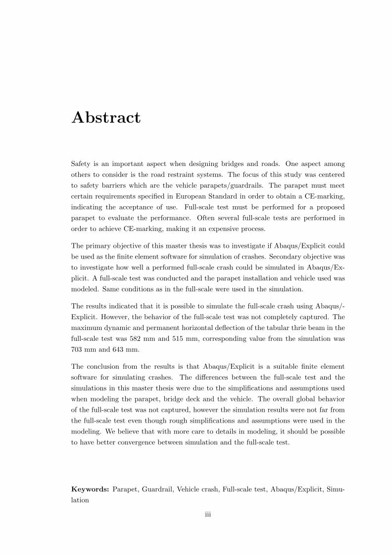
Safety is an important aspect when designing bridges and roads. One aspect among
others to consider is the road restraint systems. The focus of this study was centered
to safety barriers which are the vehicle parapets/guardrails. The parapet must meet
certain requirements specified in European Standard in order to obtain a CE-marking,
indicating the acceptance of use. Full-scale test must be performed for a proposed
parapet to evaluate the performance. Often several full-scale tests are performed in
order to achieve CE-marking, making it an expensive process.
The primary objective of this master thesis was to investigate if Abaqus/Explicit could
be used as the finite element software for simulation of crashes. Secondary objective was
to investigate how well a performed full-scale crash could be simulated in Abaqus/Ex-
plicit. A full-scale test was conducted and the parapet installation and vehicle used was
modeled. Same conditions as in the full-scale were used in the simulation.
The results indicated that it is possible to simulate the full-scale crash using Abaqus/-
Explicit. However, the behavior of the full-scale test was not completely captured. The
maximum dynamic and permanent horizontal deflection of the tabular thrie beam in the
full-scale test was 582 mm and 515 mm, corresponding value from the simulation was
703 mm and 643 mm.
The conclusion from the results is that Abaqus/Explicit is a suitable finite element
software for simulating crashes. The di↵erences between the full-scale test and the
simulations in this master thesis were due to the simplifications and assumptions used
when modeling the parapet, bridge deck and the vehicle. The overall global behavior
of the full-scale test was not captured, however the simulation results were not far from
the full-scale test even though rough simplifications and assumptions were used in the
modeling. We believe that with more care to details in modeling, it should be possible
to have better convergence between simulation and the full-scale test.
Keywords: Parapet, Guardrail, Vehicle crash, Full-scale test, Abaqus/Explicit, Simu-
lation
iii

Sammanfattning
Sakerhet ar en viktig aspekt vid utformningen av broar och vagar. En av aspekterna
som maste beaktas ar utformningen av vagracken. Dessa vagracken maste uppfylla vissa
krav som anges i Europeisk standard for att erhalla sa kallad CE-markning, som anger
godkannande av anvandning. Verkliga tester maste utforas for ett foreslaget vagracke
for att evaluera prestanda och darigenom erhalla CE-markningen. Denna process kan
bli kostsam da flera tester kan behova goras for att uppna ratt prestanda.
Syftet med detta examensarbete var att undersoka om Abaqus/Explicit kan anvandas
som finita element program for att utfora kraschsimulering och hur val en genomford
verklig krasch kan simuleras. Ett verkligt test studerades, vagracket, brobaneplat-
tan och fordonet som anvandes vid denna test modellerades i Abaqus/CAE. Samma
forutsattningar som i testet anvandes i simuleringen.
Resultaten tyder pa att det ar mojligt att simulera verkliga krascher i Abaqus/Explicit.
Det globala beteendet av testet fangades inte upp helt i simuleringen men beteendet var
dock inte allt for langt ifran. Den maximala dynamiska och permanenta horisontella
utbojningen av profilracket uppgick till 582 mm respektive 515 mm, motsvarande varde
fran simuleringen var 703 mm respektive 643 mm.
Slutsatsen ar att Abaqus/Explicit ar ett lampligt finita element program for simu-
lering av krascher. Skillnaderna mellan verkliga testet och simuleringen ar pa grund
av de forenklingar och antaganden som har gjorts vid modellering av brobaneplattan,
vagracket och fordonet. Vi tror att med mer omsorg kring detaljerna i modelleringen
gallande brobaneplattan och vagracket, bor det vara mojligt att ha en battre konvergens
mellan simuleringen och verkliga testet.
v

Contents
Preface i
Abstract iii
Sammanfattning v
Abbreviations xiii
Symbols xiv
1 Introduction 1
1.1 Background . . . . . . . . . . . . . . . . . . . . . . . . . . . . . . . . . . . 1
1.2 Aim . . . . . . . . . . . . . . . . . . . . . . . . . . . . . . . . . . . . . . . 2
1.3 Summary of previous work . . . . . . . . . . . . . . . . . . . . . . . . . . 2
1.3.1 Conclusions from previous work . . . . . . . . . . . . . . . . . . . . 3
1.4 Scope and limitations . . . . . . . . . . . . . . . . . . . . . . . . . . . . . 4
2 Finite Element Theory 5
2.1 General about Abaqus . . . . . . . . . . . . . . . . . . . . . . . . . . . . . 5
2.2 Abaqus/Explicit . . . . . . . . . . . . . . . . . . . . . . . . . . . . . . . . 6
2.3 Essential di↵erences between implicit and explicit . . . . . . . . . . . . . . 7
2.4 Automatic time incrementation and stability . . . . . . . . . . . . . . . . 8
2.4.1 Definition of the stability limit . . . . . . . . . . . . . . . . . . . . 9
2.4.2 Fully automatic time incrementation versus fixed time incremen-
tation in Abaqus/Explicit . . . . . . . . . . . . . . . . . . . . . . . 10
2.4.3 Mass scaling to control time incrementation . . . . . . . . . . . . . 11
2.4.4 E↵ect of material on stability limit . . . . . . . . . . . . . . . . . . 11
2.5 Energy balance . . . . . . . . . . . . . . . . . . . . . . . . . . . . . . . . . 12
3 Method 13
3.1 The process of the master thesis . . . . . . . . . . . . . . . . . . . . . . . 13
3.2 Full-scale crash test on the modified T8 bridge rail . . . . . . . . . . . . . 14
3.2.1 Geometry and conditions for the guardrail installation . . . . . . . 14
3.2.2 Crash test conditions . . . . . . . . . . . . . . . . . . . . . . . . . . 21
vii

Contents
3.2.3 Test vehicle . . . . . . . . . . . . . . . . . . . . . . . . . . . . . . . 21
3.3 Finite element modeling . . . . . . . . . . . . . . . . . . . . . . . . . . . . 24
3.3.1 Vehicle model . . . . . . . . . . . . . . . . . . . . . . . . . . . . . . 24
3.3.1.1 Modification of the material properties . . . . . . . . . . 25
3.3.1.2 Geometry of the vehicle model . . . . . . . . . . . . . . . 26
3.3.2 Modeling of the modified T8 bridge rail . . . . . . . . . . . . . . . 27
3.3.2.1 Modeling of the vertical posts . . . . . . . . . . . . . . . 27
3.3.2.2 Modeling of the thrie beam . . . . . . . . . . . . . . . . . 30
3.3.3 Modeling of the bridge deck . . . . . . . . . . . . . . . . . . . . . . 33
3.3.4 Assembled model . . . . . . . . . . . . . . . . . . . . . . . . . . . . 34
3.3.5 Analysis step . . . . . . . . . . . . . . . . . . . . . . . . . . . . . . 37
3.3.6 Interaction . . . . . . . . . . . . . . . . . . . . . . . . . . . . . . . 37
3.3.6.1 Contact . . . . . . . . . . . . . . . . . . . . . . . . . . . . 37
3.3.6.2 Constraints . . . . . . . . . . . . . . . . . . . . . . . . . . 38
3.3.6.3 Connections . . . . . . . . . . . . . . . . . . . . . . . . . 39
3.3.7 Load . . . . . . . . . . . . . . . . . . . . . . . . . . . . . . . . . . . 42
3.3.8 Boundary conditions . . . . . . . . . . . . . . . . . . . . . . . . . . 42
3.3.8.1 Summary of the assumptions and simplifications . . . . . 43
4 Results 44
4.1 Results of the full-scale crash test . . . . . . . . . . . . . . . . . . . . . . . 44
4.1.1 Damage to the test installation . . . . . . . . . . . . . . . . . . . . 48
4.1.2 Damage to the test vehicle . . . . . . . . . . . . . . . . . . . . . . 51
4.2 Results of the simulation . . . . . . . . . . . . . . . . . . . . . . . . . . . . 51
4.2.1 Damage to the modeled installation . . . . . . . . . . . . . . . . . 55
4.2.2 Damage to the modeled vehicle . . . . . . . . . . . . . . . . . . . . 57
4.2.3 Energy quantities . . . . . . . . . . . . . . . . . . . . . . . . . . . . 58
4.3 Qualitative comparisons . . . . . . . . . . . . . . . . . . . . . . . . . . . . 59
4.4 Quantitative comparisons . . . . . . . . . . . . . . . . . . . . . . . . . . . 66
5 Discussion and conclusions 68
6 Future work 71
Bibliography 73
Appendix A 75
A.1 Bolt connection properties . . . . . . . . . . . . . . . . . . . . . . . . . . . 75
A.2 Bending moment capacity of the post . . . . . . . . . . . . . . . . . . . . 77
Appendix B 79

Contents
B.1 Post deformations . . . . . . . . . . . . . . . . . . . . . . . . . . . . . . . 79
B.1.1 Initial angular deflection of posts 11-13 . . . . . . . . . . . . . . . 79
B.1.2 Mean angular deflection for posts 5-9 . . . . . . . . . . . . . . . . . 80
B.1.3 Angular deflection for posts 10-15 . . . . . . . . . . . . . . . . . . 80
B.1.4 Vertical deflection for posts 10-15 . . . . . . . . . . . . . . . . . . . 81
B.2 Tabular thrie beam deformations . . . . . . . . . . . . . . . . . . . . . . . 81
B.3 Vehicle position, speed and angular deflection . . . . . . . . . . . . . . . . 82

List of Figures
2.1 The di↵erence in calculation cost between implicit and explicit solver [1]. 8
3.1 Working procedure of the thesis. . . . . . . . . . . . . . . . . . . . . . . . 14
3.2 Plan view of the tested installation[2]. . . . . . . . . . . . . . . . . . . . 15
3.3 Elevation view of the tested installation[2]. . . . . . . . . . . . . . . . . . 15
3.4 Plan view of the transition zone[2]. . . . . . . . . . . . . . . . . . . . . . 15
3.5 Elevation view of the transition zone[2]. . . . . . . . . . . . . . . . . . . 16
3.6 Detail of the slotted holes[2]. . . . . . . . . . . . . . . . . . . . . . . . . . 17
3.7 Section of the tested installation[2]. . . . . . . . . . . . . . . . . . . . . . 17
3.8 Additional details of the posts[2]. . . . . . . . . . . . . . . . . . . . . . . 18
3.9 Plastic o↵set block [2]. . . . . . . . . . . . . . . . . . . . . . . . . . . . . 19
3.10 Plan and elevation view of the rebar arrangement [2]. . . . . . . . . . . . 19
3.11 Details of the rebar arrangement [2]. . . . . . . . . . . . . . . . . . . . . . 20
3.12 The complete installation prior to testing [2]. . . . . . . . . . . . . . . . . 20
3.13 Impact point and the angle between the vehicle and rail [2]. . . . . . . . . 21
3.14 The 2000 Chevrolet C2500 pickup truck used for the test [2]. . . . . . . . 22
3.15 The vehicle and installation prior the crash testing [2]. . . . . . . . . . . 22
3.16 Dimensions and other relevant distances[2]. . . . . . . . . . . . . . . . . 23
3.17 The imported vehicle in Abaqus/CAE. . . . . . . . . . . . . . . . . . . . 25
3.18 Elevation of the posts. . . . . . . . . . . . . . . . . . . . . . . . . . . . . 28
3.19 Cross section of the vertical posts. . . . . . . . . . . . . . . . . . . . . . . 29
3.20 The meshed vertical post. . . . . . . . . . . . . . . . . . . . . . . . . . . . 29
3.21 Cross section for the 12-gauged thrie beam. . . . . . . . . . . . . . . . . 31
3.22 Elevation of the thrie beam. . . . . . . . . . . . . . . . . . . . . . . . . . 31
3.23 The meshed thrie beam. . . . . . . . . . . . . . . . . . . . . . . . . . . . 32
3.24 Plan view of the bridge deck. . . . . . . . . . . . . . . . . . . . . . . . . . 33
3.25 Close up view of the notches created. . . . . . . . . . . . . . . . . . . . . 33
3.26 The assembled tabular cross section. . . . . . . . . . . . . . . . . . . . . 34
3.27 The alignment of the tabular thrie beam and the vertical post. . . . . . . 35
3.28 Vehicle position prior impact. . . . . . . . . . . . . . . . . . . . . . . . . 36
3.29 The assembled model with post numbers - isoparametric view. . . . . . . 36
3.30 Tie constraints between the two thrie beams forming the tabular thrie
beam. . . . . . . . . . . . . . . . . . . . . . . . . . . . . . . . . . . . . . . 38
3.31 Rotation center in the bridge deck. . . . . . . . . . . . . . . . . . . . . . 39
x

List of Figures
3.32 The constraints between the vertical posts and the rotational center. . . . 39
3.33 The connection between the tabular thrie beam and vertical post. . . . . . 40
3.34 The fixed boundary condition applied to the end post. . . . . . . . . . . . 42
4.1 Sequential photographs of the test, overhead and frontal view [2]. . . . . . 45
4.2 Sequential photographs of the test, overhead and frontal view (contin-
ued)[2]. . . . . . . . . . . . . . . . . . . . . . . . . . . . . . . . . . . . . . 46
4.3 Rear view of the crash[2]. . . . . . . . . . . . . . . . . . . . . . . . . . . 47
4.4 The impact point and end point of the vehicle[2]. . . . . . . . . . . . . . 48
4.5 Damage to the test installation[2]. . . . . . . . . . . . . . . . . . . . . . . 49
4.6 Permanent deformation to the test installation[2]. . . . . . . . . . . . . . 50
4.7 Vehicle after being up-righted [2]. . . . . . . . . . . . . . . . . . . . . . . 51
4.8 Sequential simulations photographs - top and front view. . . . . . . . . . 52
4.9 Sequential simulations photographs - top and front view (continued). . . 53
4.10 Sequential simulations photographs - rear view. . . . . . . . . . . . . . . 54
4.11 Deflection of the posts which experienced the largest deformations. . . . . 55
4.12 Damage to the modeled installation - front view. . . . . . . . . . . . . . . 56
4.13 Damage to the modeled installation - rear view. . . . . . . . . . . . . . . 56
4.14 Damage to the vehicle at 0.6 s. . . . . . . . . . . . . . . . . . . . . . . . 57
4.15 Energy quantities for the whole model. . . . . . . . . . . . . . . . . . . . 58
4.16 Di↵erence in the total energy for the whole model. . . . . . . . . . . . . . 59
4.17 Sequential crash photographs comparison - front view. . . . . . . . . . . . 60
4.18 Sequential crash photographs comparison - front view (continued). . . . . 61
4.19 Sequential crash photographs comparison - top view. . . . . . . . . . . . 62
4.20 Sequential crash photographs comparison - top view (continued). . . . . . 63
4.21 Sequential crash photographs comparison - rear view. . . . . . . . . . . . 64
4.22 Sequential crash photographs comparison - rear view (continued). . . . . 65
B.1 Initial angular deflection of post 11-13. . . . . . . . . . . . . . . . . . . . 79
B.2 Mean angular deflection for posts 5-9. . . . . . . . . . . . . . . . . . . . 80
B.3 Angular deflection for posts 10-15. . . . . . . . . . . . . . . . . . . . . . 80
B.4 Deflection towards field side, U2, for posts 10-15. . . . . . . . . . . . . . 81
B.5 Maximum deflection of the tabular thrie beam. . . . . . . . . . . . . . . . 81
B.6 Vehicle angle during the impact. . . . . . . . . . . . . . . . . . . . . . . . 82
B.7 Vehicle speed during the impact. . . . . . . . . . . . . . . . . . . . . . . . 82
B.8 The vehicle position and time when it was parallel to the rail. . . . . . . 83

List of Tables
3.1 Geometry of the vehicle[2]. . . . . . . . . . . . . . . . . . . . . . . . . . . . 23
3.2 Changes to some material properties of the vehicle. . . . . . . . . . . . . . 26
3.3 Geometry of the vehicle model compared to tested vehicle. . . . . . . . . . 27
3.4 Properties used for the vertical posts. . . . . . . . . . . . . . . . . . . . . . 28
3.5 Material properties used for the thrie beam. . . . . . . . . . . . . . . . . . 30
3.6 Properties of the Cartesian connector section. . . . . . . . . . . . . . . . . 40
3.7 Properties of the Cartesian+Rotation connector section. . . . . . . . . . . 41
4.1 Post deformation and deflection[2]. . . . . . . . . . . . . . . . . . . . . . . 48
4.2 Post deformation and deflection in the simulation. . . . . . . . . . . . . . 55
4.3 Post angular deflection - comparison. . . . . . . . . . . . . . . . . . . . . . 66
4.4 Post deflection - comparison. . . . . . . . . . . . . . . . . . . . . . . . . . 67
xii

Abbreviations
ASTM American Society for Testing and Materials
CAE Complete Abaqus Environment
CE Conformite Europeenne
CEN European Committee for Standardization
CFD Computational Fluid Dynamics
CIP Critical Impact Point
CORM Constrained Components of Relative Motion
DOF Degrees Of Freedom
EN European Standard
FE Finite Element
FEM Finite Element Method
FHWA Federal Highway Administration
HDPE High Density Polyethylene
INP-files Input Files
LON Length Of Need
LS-DYNA Livermore Software Dynamic Non-Linear Finite Element Program
MPC Multi-Point Constraint
NCAC National Crash Analysis Center
NCHRP National Cooperative Highway Research Program
RC Rotation Center
TL Test Level
US United States
xiii

Symbols
M Nodal mass matrix
P External forces
I Internal element forces
u Nodal displacement
u Nodal velocity
u Nodal acceleration
t Time
�t Time increment
�✏ Strain increment
✏ Strain rate
� Element stress
�tstable Stable time increment
!max Maximum eigenfrequency
⇠ Damping ratio
Le Element length
cd Material wave speed
E Young�s modulus
⇢ Mass density
EI Internal energy
EV Dissipated viscous energy
EFD Dissipated frictional energy
EKE Kinetic energy
EIHE Internal heat energy
EW External work
EPW Contact penalty work
xiv

Symbols
ECW Constraint penalty work
EMW Propelling added mass work
EHF External fluxes energy
Etotal Total energy
EE Recoverable elastic strain energy
EP Dissipated energy due to plasticity
ECD Dissipated energy due to creep
EA Artificial strain energy
EDMD Dissipated energy due to damage
EDC Dissipated energy due to distortion control
EFC Fluid cavity energy


Chapter 1
Introduction
1.1 Background
A vital part when designing bridges and roads is safety. Several aspects need to be
accounted for in order to obtain a satisfactory level of safety for the users. One aspect
among others to consider is the road restraint systems. The road restraint systems con-
sist of vehicle restraint systems and pedestrian restraint systems. The vehicle restraint
systems consist of safety barriers, terminals, transitions, removable barrier sections and
crash cushions. The focus of this study was centered to safety barriers which are the
vehicle parapets also known as guardrails. A parapet functions as a barrier or/and as a
guardrail which prevent dangerous accidents such as driving o↵ the bridge.
Di↵erent properties must be taken into consideration when these parapets are designed,
one of these properties is the global sti↵ness. The sti↵ness can neither be too high nor
too low. In a scenario where the sti↵ness of the parapet is too high it would create
great amount of damage to the vehicle and the passengers. This can be compared to
a vehicle crashing into a rigid concrete wall. In the other scenario where the sti↵ness
is too low, the parapet would snap during the impact and not fulfill its function. The
reader realizes that finding the right sti↵ness is a tightrope walk which is dependent on
several factors.
In order to be allowed to use these parapets on bridges and roads, certain requirements
must be met according to European Standards, EN, which are approved by the European
committee for standardization, CEN. The parapet obtains a Conformite Europeenne
marking, CE-marking, indicating that the parapets can be sold in EU member countries.
In order to obtain a CE-marking, full-scale tests must be performed to assess the real
behavior of the parapets. As for all real life testing it is expensive to build and perform
1

Introduction
these tests. Often more than one full-scale test is necessary to achieve CE-marking since
it is di�cult to design a parapet and its structural system to meet the requirements
in the EN standards in the first attempt. This may lead to extensive costs for the
suppliers to achieve CE-marking for the proposed parapet. To minimize these costs it is
a necessity to develop a finite element model that can simulate the crash and study the
e↵ect of di↵erent modifications of the parapets. The designer could perform simulations
in order to meet the requirements in these simulations and then perform a full-scale test
based on the dimensions used in the finite element model.
However, in order to develop a finite element model which works properly it is of great
importance to validate the model against previous full-scale crash tests. If the model
complies with the full-scale crash test, then the designer can change the geometry of
the parapet or replacing it completely and study the e↵ects of the changes in the model
before making any full-scale test on the new proposal of the parapet.
1.2 Aim
The primary objective of this master thesis was to investigate the potential of Abaqus/-
Explicit as the tool to simulate vehicle crashes into bridge parapet or parapet in general.
This study also aimed to determine how well a performed full-scale crash could be sim-
ulated in Abaqus/Explicit.
1.3 Summary of previous work
State-of-the-art reports have been reviewed in crash simulations. Generally, these reports
show that the finite element software commonly used is LS-DYNA. One of these reports
indicated that it was fully possible to make simulations in LS-DYNA that are almost
identical to the full-scale test[3]. The authors in [3] studies the bridge rail-to-guardrail
transitions. The intent of their study was twofold, firstly to accurately simulate an
observed full-scale crash test behavior and secondly to compare e↵ects of di↵erent design
alternatives that results in acceptable crash test performance in a cost-e↵ective manner.
The main reason for using LS-DYNA was that it is a software well established for
simulations involving high speed dynamics. Another advantage of using LS-DYNA was
the accessibility of adapted vehicle models. There are several vehicle models available at
the website of National Crash Analysis Center, NCAC, these models are developed for
use in LS-DYNA[4]. The vehicle models were developed and validated using multiple
impact data as mentioned in [3], crucial part for these vehicles were modeled through a
2

Introduction
detailed component testing program at NCAC. The C-2500 pickup truck vehicle model
has been used in previous finite element studies and it was demonstrated that this vehicle
model was fairly accurate in representing impact simulations[3].
A technical report written by Nauman M. Sheikh et al. was reviewed where finite element
simulations were performed for several guardrail systems. LS-DYNA was used as the
finite element software. The technical report was produced as a product of a research
to develop finite element simulations as the tool to evaluate the performance of selected
roadside safety devices subjected to very high-speed impacts[5]. The finite element
models developed for the di↵erent guardrail systems used in [5] were very detailed. The
authors considered details ranging from the connections including bolts to the post-soil
interaction. The vehicle models used in [5] were the C2500 pickup, similar to the one used
in [3], and a small passenger car. These vehicles were from the NCAC, however slightly
modified and improved by the authors in order to further reflect the true behavior of the
real pickup truck[6]. As in previous report, [3], the authors in [5] manage to simulate a
full-scale test with great precision.
Reports regarding Abaqus/Explicit as the finite element tool instead of LS-DYNA for
crash simulations have been reviewed in order to determine the crashworthiness of
Abaqus/Explicit. Reports such as [7] indicated that Abaqus/Explicit is fully capable to
simulate the behavior of full-scale test given su�cient care for key properties.
In 2012 Simulia published a paper from the 2012 Simulia Community Conference where
crash simulations in Abaqus/Explicit were performed. Comparison with a full-scale
crash test was presented in [8]. This paper indicated that it should be possible to
simulate and have good correlation with full-scale test if relevant details were modeled
properly. The authors in [8] paid a lot of attention to the soil-post interaction and the
connection of the guardrail to the post. However, the authors did not mention how the
vehicle model was converted from a LS-DYNA model from the website of NCAC to an
Abaqus CAE model.
1.3.1 Conclusions from previous work
Conclusions from the state-of-the-art study are listed below:
• There is no ”ready-to-go” vehicle model adapted for the Abaqus/Explicit.
• The mass and geometry of the vehicle is of great importance.
• The vertical post and the thrie-beam should be modeled using shell element to
reflect the true behavior of these parts.
3
Introduction
• The connection between the vertical posts and thrie-beam should be given su�cient
care.
• The interaction between the bottom of the vertical post and surrounding areas
such as the soil or pavement should also be addressed.
• Friction between the vehicle tires and the pavement should reflect reality.
• Small enough mesh should be used for areas in contact to avoid penetration.
• The simulations should always be validated against full-scale crash test.
The main problem when using Abaqus/Explicit as the finite element software is that
there is no vehicle model available today. Realistic vehicle model is a must in order to
obtain results from simulations that are close to the full-scale crash test.
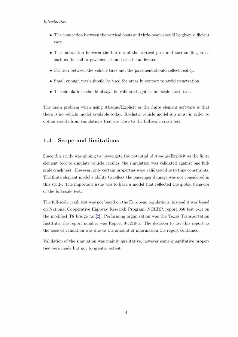
1.4 Scope and limitations
Since this study was aiming to investigate the potential of Abaqus/Explicit as the finite
element tool to simulate vehicle crashes, the simulation was validated against one full-
scale crash test. However, only certain properties were validated due to time constraints.
The finite element model’s ability to reflect the passenger damage was not considered in
this study. The important issue was to have a model that reflected the global behavior
of the full-scale test.
The full-scale crash test was not based on the European regulations, instead it was based
on National Cooperative Highway Research Program, NCHRP, report 350 test 3-11 on
the modified T8 bridge rail[2]. Performing organization was the Texas Transportation
Institute, the report number was Report 0-5210-6. The decision to use this report as
the base of validation was due to the amount of information the report contained.
Validation of the simulation was mainly qualitative, however some quantitative proper-
ties were made but not to greater extent.
4

Chapter 2
Finite Element Theory
Finite Element Method, FEM, is a numerical calculation method which solves various
di↵erential equations with the aid of a computer. FEM divide a continuum into a finite
number of elements. The characteristic feature of FEM is that instead of solving the
di↵erential equation for the whole continuum, they are solved approximately for the
finite elements. The elements are connected at nodes holding the elements together.
The nodal points are the ends of the each element, each node has a number of degrees of
freedom, DOF, such as translation and rotation in x and y for a 2D analysis and x, y and
z-direction for a 3D analysis. From the values of the nodal DOF’s the element behavior
can be determined in a controlled manner with the aid of predefined equations, and
since the mechanical behavior of the material is known, the corresponding mechanical
behavior of each element is determined. This is performed for every single element
forming the continuum allowing the possibility to obtain an approximate solution for
the entire continuum.
2.1 General about Abaqus
Abaqus is a finite element program originally developed by Dassault Systemes. Abaqus is
a suite of engineering simulation programs that can solve problems ranging from simple
linear analysis to highly complex nonlinear dynamic simulations. It consists of wide
range of elements which make it possible to model any type of geometry. It has a broad
list of material models that can be used to simulate material behavior of interest such
as steel, concrete, aluminum, geotechnical materials such as soils and rock and other
materials not mentioned here. In a nonlinear analysis Abaqus automatically chooses
and adjust the load increment and convergence tolerance during the analysis to ensure
that an accurate solution is obtained.
5

Finite Element Theory
Abaqus consists of three main analysis products each one of them suitable for di↵erent
physical problems. These analysis products are Abaqus/Standard, Abaqus/Explicit and
Abaqus/CFD. Abaqus/Standard is a general-purpose analysis that can solve linear and
nonlinear problems involving static, dynamic and other type of engineering problems,
the standard uses the implicit method to solve the problems. Abaqus/Explicit is an
analysis product used in special-purpose, this product uses an explicit dynamic finite
element formulation. It is suitable for brief, transient dynamic events, such as impact
problems. It is also preferred for problems involving large deformations, i.e. highly
nonlinear problems. Abaqus/CFD is used to study fluid dynamics[9].
Since this master thesis involves impact analysis with large deformation Abaqus/Ex-
plicit is deemed suitable.
2.2 Abaqus/Explicit
Abaqus/Explicit uses, as the name indicate, explicit methods to integrate through time.
The explicit method used is the central di↵erence method, which integrate the equations
of motion through time. It uses kinematic conditions at one increment to calculate the
kinematic conditions at the next increment. When the solver is initiated it solves for
the dynamic equilibrium[10], equation 2.1,
Mu = P� I (2.1)
where:
M, is nodal mass matrix,
P, I, are the external applied forces and internal element forces,
u, is the nodal acceleration.
From equation 2.1 the nodal accelerations are obtained in the beginning of the current
increment, time t, as
u|(t) = M
�1(P� I)|(t). (2.2)
The explicit solver uses lumped mass matrix, a diagonal mass matrix, which makes the
calculations for accelerations elementary. There are no simultaneous equations to solve,
the nodal acceleration of any node is determined by its mass and the net force acting
on it, resulting in inexpensive calculations.
6
Finite Element Theory
Nodal velocities are calculated through the known nodal accelerations. Nodal acceler-
ations are integrated through time using central di↵erence rule. Change in velocity is
calculated assuming that the acceleration is constant, this change of the velocity is then
added to the velocity from middle of the previous increment to determine the velocity
at the middle of current increment:
u|(t+�t
2
) = u|(t��t
2
) +�t|(t+�t) +�t|(t)
2u|(t) (2.3)
When the nodal velocities are calculated, the solver integrates these velocities in order
to obtain the nodal displacement as:
u|(t+�t) = u|(t) +�t|(t+�t)u|(t+�t
2
) (2.4)
As mentioned above, the explicit method assumes constant acceleration for each incre-
ment. In order to obtain results that are accurate, su�ciently small time increments
must be used in order to have nearly constant accelerations during an increment result-
ing in analysis with large number of increments. However, each increment is inexpensive
since there are no simultaneous equations to solve.
Knowing the nodal displacement, the solver initiates element calculations. The element
strain increments, �✏, are computed from the strain rate, ✏. The computed strain
increment makes it possible to compute the element stresses, �, by applying the material
constitutive relationships i.e. the element sti↵ness. Symbolically this could be written
as:
�(t+�t) = f(�(t),�✏) (2.5)
and consequently, internal forces are assembled, I(t+�t).
The process described above is performed for each time increment, when all above men-
tioned steps are applied for the current increment the process is repeated for the next
increment by setting the new time, t, to t = t+�t and returning to equation 2.2.
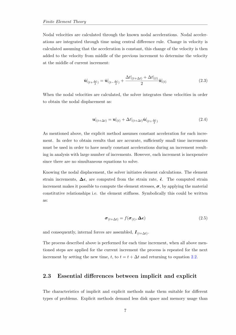
2.3 Essential di↵erences between implicit and explicit
The characteristics of implicit and explicit methods make them suitable for di↵erent
types of problems. Explicit methods demand less disk space and memory usage than
7
Finite Element Theory
the implicit solver, which is partly due to that no iteration is performed within each
time step and partly due to the usage of the diagonal, lumped mass matrix, the system
to be solved is uncoupled. The convergence problem that may be present in implicit
methods can be avoided with an explicit method[11]. The greatest feature of the explicit
method is the absence of a global tangent sti↵ness matrix, which is required with implicit
methods. Since the state of the model is advanced explicitly, iterations and tolerances are
not required[12]. Another advantage of explicit method over the implicit one is the cost
of calculations due to increase number of DOF:s. The di↵erence is shown schematically
in Figure 2.1.
Figure 2.1: The di↵erence in calculation cost between implicit and explicit solver [1].
2.4 Automatic time incrementation and stability
As mentioned in Section 2.2, the time incrementation is vital for the Explicit solver
to be stable. It is the stability limit that dictates the maximum time increment used,
making it the critical factor for the performance of Abaqus/Explicit. The Explicit solver
is conditionally stable meaning that the amount of time that the state of the simulation
can be advanced and still remain accurate is short. If the time increment is larger than
this maximum amount of time, the increment is said to have exceeded the stability limit.
Exceeding the stability limit results in unbounded solutions[13]. Generally it is not
easy to determine the stability time exactly, conservative estimates are used instead.
Since the stability limit has great influence on reliability and accuracy, it must always
be determined consistently and conservatively. However, the time increment cannot
be arbitrarily small due to computational e�ciency. Abaqus/Explicit chooses the time
increments to be as close as possible to the stability time limit without exceeding it.
8

Finite Element Theory
2.4.1 Definition of the stability limit
The stability limit is defined in terms of the highest circular frequency in the system,
!max. Without considering damping for the system the stability limit is calculated as
�tstable =2
!max, (2.6)
and if damping is considered the expression above becomes
�tstable =2
!max
⇣p1 + ⇠2 � ⇠
⌘, (2.7)
where ⇠ is the fraction of the critical damping in the mode with the highest frequency.
From basic dynamics it is known that critical damping is defined as the limit between
oscillatory and non-oscillatory motion in the context of free-damped vibration. It should
be mentioned that Abaqus/Explicit always introduces a small amount of damping in the
form of bulk viscosity to control high-frequency oscillations[14].
However, to determine the actual highest frequency in the system is based on a complex
set of interacting factors and the task is not computational feasible to calculate its exact
value. An estimate which is simple, e�cient and conservative is used. Instead of looking
at the global model, the highest frequency of each individual element in the model is
estimated. This frequency is always associated with the dilatational mode. It is shown
that the highest element frequency determined on an element-by-element basis is always
higher than the highest frequency in the assembled finite element model[14]. Given the
fact in the previous sentence the stability limit defined in expression 2.7 can be based on
element-by-element basis and be redefined using the element length, Le, and the wave
speed of the material, cd, as
�tstable =Le
cd. (2.8)
It is clear that the shorter the element length, the smaller stability limit. The wave
speed is a property of the material. For linear elastic material with Poisson’s ratio of
zero the wave speed is defined as
cd =
sE
⇢, (2.9)
where E is Young’s modulus and ⇢ is the mass density.
9

Finite Element Theory
The simplified stability limit makes it possible to predict the stability limit given the
smallest element length and material. For example a material with a wave speed of 5000
m/s (close to steel) and with the smallest element dimension of 100 mm, the stability
limit is 2⇥ 10�5 s.
2.4.2 Fully automatic time incrementation versus fixed time incremen-
tation in Abaqus/Explicit
The equations discussed in Section 2.4.1 are used in Abaqus/Explicit to adjust the
time increment size throughout the analysis so that the stability limit, based on the
current state of the model, is never exceeded. Time incrementation is automatic and
requires no user intervention, not even a proposal for the initial time incrementation.
The stability limit is a mathematical concept resulting from the numerical model. The
Explicit solver has all the relevant details needed and can determine an e�cient and
conservative stability limit. However, it is possible for the user to override the automatic
time incrementation if desired.
If the automatic time incrementation is overridden the user must choose the time incre-
ment with caution. Failure to use small enough time increment will result in unstable
solution. The time history response of solution variables such as displacement will usu-
ally oscillate with increasing amplitudes when instability is at hand. The total energy
will also change significantly.
In nonlinear problems - problems with large deformation and with nonlinear material
response, as in this master thesis, the highest frequency of the model will continually
change resulting in change of the stability limit. Abaqus/Explicit has two strategies
for time incrementation control, fully automatic time incrementation, where the code
accounts for changes in the stability limit, and fixed time incrementation[15].
Two types of estimates are used for automatic time incrementation in order to deter-
mine the stability limit: element-by-element and global. Every analysis starts with the
element-by-element estimation method and may switch to the global estimator given cer-
tain circumstances during the analysis. The element-by-element is conservative, meaning
that it will produce a smaller stable time increment than the true stability limit based
upon the maximum frequency of the entire model. It is of great importance to know
that constraints such as boundary conditions and kinematic contact have the e↵ect of
compressing the eigenvalue spectrum which is not taken into account by the element-
by-element estimator.
10

Finite Element Theory
The global estimation algorithm determines the maximum frequency of the entire model
using current dilatational wave speed. This algorithm continuously updates the max-
imum frequency to have accurate stability limit. The global estimator will usually
allow for time increments that exceeds the values determined by the element-by-element
estimator[15].
A fixed time incrementation procedure is also available, the fixed time increment size is
determined by the initial element-by-element stability estimate for the step or by a time
increment specified by the user.
2.4.3 Mass scaling to control time incrementation
Since the mass density have great influence on the stability limit, it may be useful to
enlarge the mass density for certain elements under some circumstances. Scaling the
mass density can potentially increase the e�ciency of the analysis. Due to the complex
discretization of models, there are often regions containing very small or poorly shaped
elements that control the stability limit of the entire model. These elements may be few
and only exists at localized areas. The stability limit may increase significantly while
e↵ect on the overall dynamic behavior is negligible if the mass of these elements are
increased.
There are two ways of applying mass scaling: defining a scaling factor directly or defining
a desired element-by-element stable time increment for specific elements that are of poor
shape. These two approaches allows for additional user control over the stability limit.
However, the user must be careful and absolutely certain that scaling these elements
does not change the overall behavior of the system[16].
2.4.4 E↵ect of material on stability limit
The material model used will a↵ect the stability limit through its e↵ect on the dilata-
tional wave speed. In a linear elastic material the Young’s modulus is constant and the
only factor a↵ecting the stability limit during the analysis is the change in the smallest
element dimension. In a nonlinear material, such as steel with plasticity, the wave speed
changes as the materials start to yield and the sti↵ness of the material decreases. This
e↵ect results in a increase of the stability limit.
11

Finite Element Theory
2.5 Energy balance
Energy output is a vital part in Abaqus/Explicit analysis. Energy output comprises
of several components, comparison between these various energy components is used to
evaluate whether the analysis is having appropriate response.
The energy balance for the entire model can be written as
EI +EV +EFD +EKE +EIHE �EW �EPW �ECW �EMW �EHF = Etotal, (2.10)
where EI is the internal energy, EV is the viscous energy dissipated, EFD is the frictional
dissipated energy, EKE is the kinetic energy, EIHE is the internal heat energy, EW is
the work done by the external applied loads and EPW , ECW and EMW are the work
done by contact penalties, constraint penalties and propelling added mass respectively.
EHF is the external energy through external fluxes. The sum of these components is
Etotal, which should be constant. However, for numerical models this is seldom the case,
Etotal is only approximately constant, generally with an error of 1%[17].
The internal energy component, EI , in equation 2.10 is in turn composed of several
other components. The expression for the internal energy is
EI = EE + EP + ECD + EA + EDMD + EDC + EFC , (2.11)
where EE is the recoverable elastic strain energy, EP is the dissipated energy through
inelastic processes such as plasticity, ECD is the dissipated energy through viscoelasticity
or creep, EA is the artificial strain energy, EDMD is the dissipated energy through
damage, EDC is the dissipated energy through distortion control, EFC is the fluid cavity
energy[17].
An important aspect to consider with extra care is the artificial strain energy. The
artificial strain energy includes the energy stored in hourglass resistances and transverse
shear in shell and beam elements. In order to decide whether a mesh refinement is
required or not the artificial strain energy should be studied. Large values of artificial
strain energy indicate that refinement or changes should be made.
12

Chapter 3
Method
This chapter is intended as a recipe of this master thesis. The chapter starts with the
process of the approach used in the thesis. The approach is followed by the description
of the characteristic features of the full-scale test used. After that, the main steps in the
finite element modeling are described followed by a summary of the assumptions and
simplifications made in this thesis.
3.1 The process of the master thesis
In order to examine the possibility of Abaqus/Explicit as the tool to simulate a full-scale
test, it was a necessity to have a technical report of the full-scale test. The technical
report used in this master thesis was report 350 test 3-11, on the modified T8 bridge rail
as mentioned in section 1.4, which will be referenced as the full-scale test hereafter. This
technical report was used as the base for the finite element modeling and simulation. The
simulation performed was validated against some of the results of test 3-11. Drawings of
the guardrail were provided by the technical report of the full-scale test and the bridge
rail was modeled using Abaqus CAE.
13

Method
The approach for this master thesis is schematically illustrated in Figure 3.1.
Figure 3.1: Working procedure of the thesis.
However, it should be noticed that the procedure displayed in Figure 3.1 was highly
iterative. When non satisfactory results were obtained in one step the process was
repeated by going back to the previous step to search for key properties that could
have influenced. Information and knowledge needed in di↵erent steps were collected
along the process through previous works, technical reports, handbooks, supervisors
and other master theses.
3.2 Full-scale crash test on the modified T8 bridge rail
The test was sponsored by the Federal Highway Administration, FHWA, and the test
was intended to evaluate the impact performance of the modified T8 rail bridge. The
crash testing was performed in accordance with the requirements of NCHRP Report
350 Test Level 3 (TL-3). The modified T8 rail was intended to serve as the replacement
for the Texas Type T6 rail for high-speed applications on culverts and thin bridge deck
structures[2].
3.2.1 Geometry and conditions for the guardrail installation
Since the test was performed in US, all the dimensions given for di↵erent parts in this
section are given in US units. The modified T8 bridge rail installation consisted of
a 12 gauged tubular thrie-beam rail vertically supported by W6x8.5 steel posts. The
reader should notice that the dimensions used are American standard dimensions. The
vertical posts were anchored to a 6.5-inch (approx. 165 mm) thick cantilever concrete
deck. The length of the modified T8 bridge rail section and the cantilevered bridge deck
constructed and tested was 97 ft. - 9 inches (approx. 29.8 m). A plan view of the
installation is shown in Figure 3.2.
14

Method
Figure 3.2: Plan view of the tested installation[2].
The rail was end anchored with ET plus end terminal at each end, making the overall
length of the test installation 137 ft. - 6-inches (approx. 41.91 m) as shown in Figure 3.2.
The terminals were connected to the tubular thrie beam through a standard 12 gauged
thrie-beam to W-beam transition rail elements. The transition is shown in Figure 3.4
and Figure 3.5
Figure 3.3: Elevation view of the tested installation[2].
Figure 3.4: Plan view of the transition zone[2].
15

Method
Figure 3.5: Elevation view of the transition zone[2].
The steel post were welded to a 12-inch x 9.5-inch x 1-inch thick (approx. 305x240x25
mm) base plate. Two 0.25-inch (6.35 mm) wide by 1-inch (25.4 mm) long slots were
machine cut into the tra�c sided flange of the posts, the position of these slots was
located 0.75-inch (19.05 mm) above the top face of the base plate, see Figure 3.6. Each
steel post with base plate was anchored to the cantilever concrete deck using 0.875-
inch (approx. 22 mm) ASTM A307 anchor bolts as shown in Figure 3.7. Additional
information for the steel posts are shown in Figure 3.8.
16

Method
Figure 3.6: Detail of the slotted holes[2].
Figure 3.7: Section of the tested installation[2].
17

Method
Figure 3.8: Additional details of the posts[2].
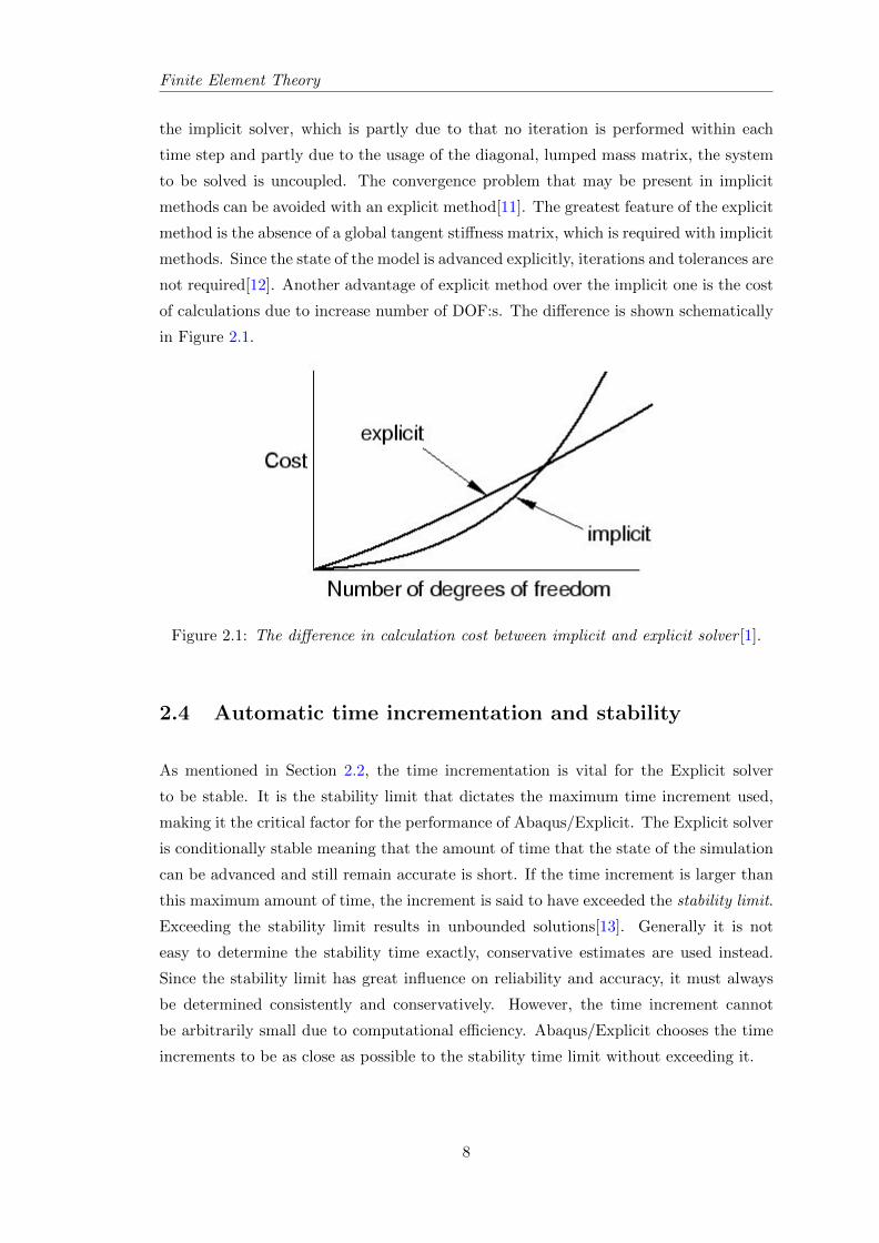
The tabular thrie beam was anchored to the vertical post using 0.625-inch (15.875 mm)
diameter x 3-inch (76.2 mm) long, ASTM A307 bolts. The bolts were mounted through
a 0.75-inch (19.05 mm) pipe sleeve. A 5-inch wide x 11-1/4-inch long x 1-1/4-inch
deep (127x285.75x31.75 mm) high density polyethylene (HDPE) o↵set block was placed
between the post and the field side of the tubular thrie beam rail as illustrated in Figure
3.7, the geometry of the o↵set block is shown in Figure 3.9. This provided a 1-inch (25.4
mm) o↵set distance between the posts and the thrie beam.
The width of the cantilevered deck was 30 inches (762 mm). The rebar arrangement
in the concrete deck is shown in Figure 3.10 and Figure 3.11. All the rebars had 60
ksi (414 MPa) yield point. The specified 28-day compressive strength for the concrete
cantilevered deck was 3000 psi (approx. 20.7 MPa). The actual compressive strength of
the concrete deck on the day the test was performed was 3536 psi (approx. 24.4 MPa)[2].
All steel plates and structural members meet A36 material specifications. Photographs
of the completed test installations is shown i Figure 3.12.
18
Method
Figure 3.9: Plastic o↵set block [2].
Figure 3.10: Plan and elevation view of the rebar arrangement [2].
19

Method
Figure 3.11: Details of the rebar arrangement [2].
Figure 3.12: The complete installation prior to testing [2].
20

Method
3.2.2 Crash test conditions
NCHRP Report 350 test 3-11 involves a 4409-lb (approx. 2000 kg) pickup truck im-
pacting the critical impact point, CIP, in the length of need, LON, of the longitudinal
barrier at a nominal speed of 62 mi/h (approx. 99.8 km/h) and with an impact angle
of 25 degrees. The test was intended to evaluate the strength of the rail in terms of its
ability to contain and redirect the pickup truck[2].
Critical impact point for the T8 rail was chosen to 1.5 ft. upstream of post 11 which
corresponds to the 7th bridge rail post. Selection of CIP was in accordance with the
guidelines in NCHRP Report 350.
The actual speed and angle for this particular test was measured to 62.1 mi/h (99.9
km/h) and 23.8 degrees. Actual impact point was 20-inch (508 mm) of post 11 as shown
in Figure 3.13.
Figure 3.13: Impact point and the angle between the vehicle and rail [2].
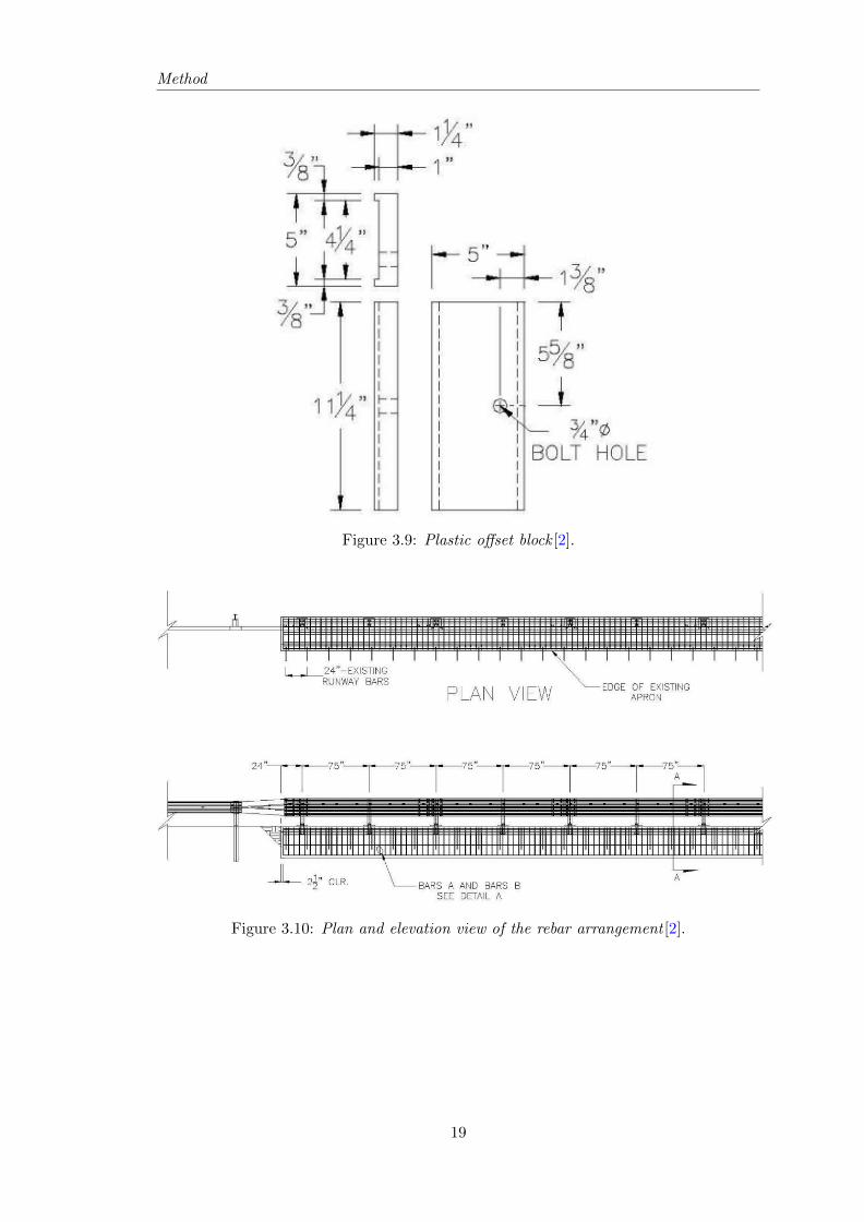
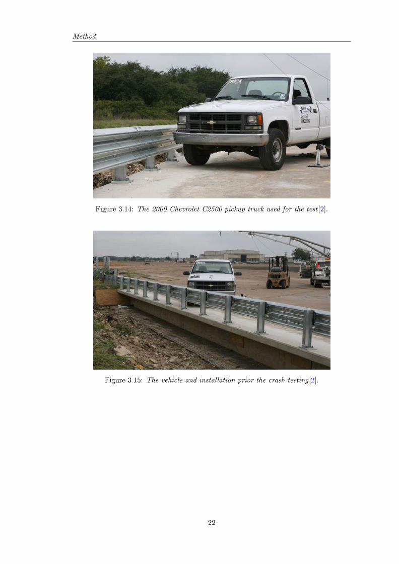
3.2.3 Test vehicle
The vehicle used for the test was a 2000 Chevrolet C2500 pickup truck shown in Figure
3.14 and Figure 3.15. The test inertia weight of the car was 4522 lb (approx. 2051 kg),
and its gross static weight was also 4522 lb[2]. Relevant dimensions and information of
the vehicle is found in Figure 3.16 and Table 3.1. More specifications for the vehicle
can be found in APPENDIX B of [2]. The vehicle was accelerated into the installation
using a cable reverse tow and guidance system, and was released to be free-wheeling and
unrestrained just prior to impact.
21
Method
Figure 3.14: The 2000 Chevrolet C2500 pickup truck used for the test [2].
Figure 3.15: The vehicle and installation prior the crash testing [2].
22

Method
Figure 3.16: Dimensions and other relevant distances[2].
Table 3.1: Geometry of the vehicle[2].
Character Inch and [mm] Character Inch and [mm]
A 74 [1880] B 32 [813]
C 32 [3353] D 71.5 [1816]
E 51.5 [1308] F 215.35 [5470]
G 57.49 [1460] H Not mentioned in [2]
J 41 [1041] K 25 [635]
L 2.75 [70] M 16.25 [413]
N 62.5 [1588] O 63.4 [1610]
P 28.5 [724] Q 17.25 [438]
R 29.5 [749] S 35.5 [902]
T 57.5 [1461] U 132.25 [3359]
23

Method
3.3 Finite element modeling
Modeling and analysis of the impact were carried out in Abaqus/CAE and Abaqus/Ex-
plicit. The modeling was performed in the CAE while the analysis was performed using
the Explicit solver.
In order to increase the reliability of the results obtained in Abaqus, smaller models that
could be verified prior to the full analysis were made. For example a cantilever beam
with a point load at the tip was modeled to compare with simple hand calculations in
order to assure compliance. This process was applied throughout the entire modeling
process to assure that the model behaved as intended.
Finite element modeling was carried out as a parallel process as mentioned in Figure 3.1.
The vehicle model was modeled along the modified T8 bridge rail to make the modeling
process as short as possible. When satisfactory models for the purpose of this thesis
were developed for the parapet/guardrail and the vehicle, the models were assembled to
one final model. The final model was used to carry out the simulation.
In the following sections, the modeling and the inputs used in Abaqus/CAE are presented
together with the assumptions and simplifications.
3.3.1 Vehicle model
Vehicle model used for this thesis was a pick-up truck, a 1994 Chevrolet C1500. This
model was used due to the similarities of the vehicle used for the full-scale crash test
described above. Simulia obtained the model geometry, element connectivity, and ma-
terial properties from the Public Finite Element Model Archive of the National Crash
Analysis Center at George Washington University.
However the model was not a complete model ready to use in Abaqus simulations. The
model was organized as a collection of individual parts connected together. For each
part of the vehicle there were several input files, INP-files, which forms the geometry,
material properties and the connectivity to adjacent parts.
These INP-files were found in the Abaqus 6.14 Documentation[18]. The input files are
formed as scripts containing the nodes, element types, sections and connections of the
parts. The INP-files were parametrized which means that they read values from another
input file where di↵erent parameters are defined. The input reader in Abaqus does not
support parametrized input files which read the parameters from another INP-files, it
can only read parameters defined in the same INP-file. This obstacle enforced us to
replace all the parameters in the INP-files and instead use the values defined in the
24
Method
parameter file. Several problems beside the parameter problem were encountered. Some
of these problems were that the beam section and rotary inertia definition in the INP-
files was not supported by the input reader. All these problems were solved with the
aid of Abaqus Scripting Reference Guide. Once all the modifications necessary were
made to the original INP-files downloaded from [18], the vehicle geometry, properties
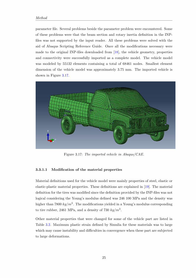
and connectivity were successfully imported as a complete model. The vehicle model
was modeled by 55132 elements containing a total of 68461 nodes. Smallest element
dimension of the vehicle model was approximately 3.75 mm. The imported vehicle is
shown in Figure 3.17.
Figure 3.17: The imported vehicle in Abaqus/CAE.
3.3.1.1 Modification of the material properties
Material definitions used for the vehicle model were mainly properties of steel, elastic or
elastic-plastic material properties. These definitions are explained in [19]. The material
definition for the tires was modified since the definition provided by the INP-files was not
logical considering the Young’s modulus defined was 246 100 MPa and the density was
higher than 7800 kg/m3. The modifications yielded in a Young’s modulus corresponding
to tire rubber, 2461 MPa, and a density of 730 kg/m3.
Other material properties that were changed for some of the vehicle part are listed in
Table 3.2. Maximum plastic strain defined by Simulia for these materials was to large
which may cause instability and di�culties in convergence when these part are subjected
to large deformations.
25

Method
Table 3.2: Changes to some material properties of the vehicle.
Material Name Maximum
Yield Stress
[MPa]
Maximum
Plastic Strain
(Old value) [-]
ELASTICPLASTIC1 449 0.3 (2.398)
ELASTICPLASTIC2 504 0.3 (2.398)
ELASTICPLASTIC-ARM 449 0.3 (2.398)
ELASTICPLASTIC-OUTER-RIM 449 0.3 (2.398)
Once the vehicle was imported to Abaqus/CAE and the material modification was ap-
plied as described above, a comparison with the vehicle used in the full-scale test was
performed in order to assess the modifications that were required to have good enough
similarities between the vehicle model and the test vehicle. The first assessment was to
determine the mass of the modeled vehicle and compare it to the vehicle used in the
full-scale test.
The assessment showed that the mass of the vehicle model was approximately 1798 kg
compared to 2051 kg for the test vehicle. In order to have same kinetic energy for the
modeled as for the tested vehicle, the mass of the model was increased with 12 %. This
increase was applied through the densities defined in the material properties of Abaqus/-
CAE. The outcome of this adjustment was an increase of the mass to approximately 2014
kg.
3.3.1.2 Geometry of the vehicle model
This section serves as a comparison in the geometry and relevant distances between the
vehicle model and the tested vehicle. Some values of corresponding dimensions listed in
Table 3.1 are listed in Table 3.3.
Most important dimension to compare was ”R” where the center of gravity was located
for the vehicle in the vertical direction. The vehicle model had some di↵erence compared
to the tested vehicle. However the di↵erence was small enough for the purpose of this
master thesis. Another dimension that might influence the behavior of the vehicle was
”T”, where the di↵erence was large. This di↵erence could be due to the densities used
for the engine and adjacent parts of the modeled vehicle model were higher than for
the corresponding parts in the tested vehicle, resulting in a displaced gravity center
towards the front wheels. After consulting with the supervisors of this master thesis, it
was judged that it was more important to have good correspondence with the dimension
”R” than ”T” and that the vehicle model was good enough for the purpose of this study.
26

Method
Table 3.3: Geometry of the vehicle model compared to tested vehicle.
Character Tested Vehicle [mm] Modeled Vehicle [mm] � [mm]
A 1880 1876 3
B 813 915 102
C 3353 3365 12
D 1816 1843 27
E 1308 1177 131
F 5470 5457 13
J 1041 1025 16
K 635 657 22
L 70 88 18
M 413 442 29
P 724 718 6
Q 438 417 21
R 749 710 39
T 1461 1215 246
3.3.2 Modeling of the modified T8 bridge rail
The finite element modeling of the modified T8 bridge rail was constructed by two parts,
the vertical posts and the thrie beam. These two parts are described in the following
subsections where relevant dimensions are shown together with other relevant geometric
properties.
3.3.2.1 Modeling of the vertical posts
The vertical posts were created in the Part Module of Abaqus/CAE. The part type was
selected to deformable with the shell extrusion base feature. The cross section of the
posts was created in the sketch feature of Abaqus/CAE. The sketched dimensions were
according to Figure 3.19a which resulted in the cross section shown in Figure 3.19b.
The length of the post was obtained by extruding the cross section with 775 mm. The
material properties used for the posts are tabulated in Table 3.4. Two homogeneous
shell sections were created and assigned to the post, one for the web with a thickness
of 4.3 mm and another for the flanges with a thickness of 4.9 mm. A final global mesh
size of 12.5 mm was assigned to the post, shown in Figure 3.20.
27

Method
Table 3.4: Properties used for the vertical posts.
Steel Post Properties Abaqus Input
Material type Piecewise linear plastic material
Element type A 4-node shell (S4R), default hourglass control.
E-modulus [MPa] 200 000
Yield Stress [MPa] 250
Density [t/mm3] 7.85E-09
Possion’s Ratio 0.26
True Stress [MPa] 250 475
E↵ective Plastic Strain 0.00 0.20
Elevation of the post is shown in Figure 3.18 and the cross section of the modeled
post is shown in 3.19. A partition face was created in order to create geometric nodes
which were used when connecting the thrie beam with the vertical posts, the connection
between the thrie beam and vertical posts are discussed in Section 3.3.6.3.
(a) Dimensions used for the posts.(b) Elevation of the post inAbaqus/CAE
Figure 3.18: Elevation of the posts.
28

Method
(a) Dimensions used for thecross section.
(b) Modeled cross section inAbaqus/CAE
Figure 3.19: Cross section of the vertical posts.
Figure 3.20: The meshed vertical post.
29

Method
3.3.2.2 Modeling of the thrie beam
The geometry of the thrie beam was created using the same procedure as for the vertical
post, described in Section 3.3.2.1. The geometry of the thrie beam was created based
on the blueprint shown in Figure 3.21a. The dimensions were standard dimension of a
12 gauged thrie beam which was used in the full-scale test. The modeled cross-section
in Abaqus/CAE is shown in Figure 3.21b. The cross section was then extruded with a
distance of 35660 mm, see Figure 3.22. Partitions with a center distance of 1905 mm
were created along the length of the thrie beam starting from an edge distance of 3780
mm from left end and ending a distance of 1880 mm from the right end if Figure 3.22
is used as reference. The partitioning was necessary in order to create geometric nodes
which were used for the connection to the vertical posts.
The material properties used for the thrie beam are tabulated in Table 3.5. A homo-
geneous shell section with a thickness of 5 mm was created and assigned to the thrie
beam. A final global mesh size of 10 mm was assigned to the thrie bream, shown in
Figure 3.23.
Table 3.5: Material properties used for the thrie beam.
Steel Post Properties Abaqus Input
Material type Piecewise linear plastic material
Element type A 4-node shell (S4R), default hourglass control.
E-modulus [MPa] 200 000
Yield Stress [MPa] 250
Density [t/mm3] 7.85E-09
Possion’s Ratio 0.26
True Stress [MPa] 250 475
E↵ective Plastic Strain 0.00 0.20
30

Method
(a) Blueprint of the cross section. (b) Modeled cross section in Abaqus/CAE
Figure 3.21: Cross section for the 12-gauged thrie beam.
Figure 3.22: Elevation of the thrie beam.
31

Method
Figure 3.23: The meshed thrie beam.
32

Method
3.3.3 Modeling of the bridge deck
The cantilevered bridge deck with all the rebars and details was not modeled in this
thesis due to lack of time. Instead, a discrete rigid body was created to represent the
deck. This part was created in the part module of Abaqus/CAE and the solid extrusion
base feature was used. The dimensions used were 15000 x 30000 mm with a extrusion of
165 mm, a plan view of the deck is shown in Figure 3.24. Notches with dimension of 110 x
198 mm were created where the vertical posts were located in order to permit rotation of
the vertical post when impacted, the notches are shown in Figure 3.25. Center distance
of the notches was 1905 mm as for the vertical posts.
Figure 3.24: Plan view of the bridge deck.
Figure 3.25: Close up view of the notches created.
33

Method
3.3.4 Assembled model
When all the necessary parts required for the simulation were created, a complete model
could be assembled. Prior to the assembly, a copy of the thrie beam part was created
to assemble the tabular thrie beam as shown in Figure 3.26.
Figure 3.26: The assembled tabular cross section.
In the completed finite element model, only the vertical post 5-20 shown in Figure 3.3
were modeled. The vertical posts were positioned with a center distance of 1905 mm.
The transition zones of the test installation were not modeled, instead the tabular thrie
beam was extended beyond post 5 and 20 with a distance of 3780 mm respectively 1880
mm and additional vertical post was placed at each end of the tabular thrie beam where
boundary conditions were applied, see Section 3.3.8. The tabular thrie beam and the
vertical post were positioned according to Figure 3.27. The vertex of the tabular thrie
34

Method
beam was 787.7 mm from the top of bridge deck. The horizontal distance between
vertical post and the tabular thrie beam was 85.45 mm and is represented by the dotted
blue line in Figure 3.27. The discrete rigid body representing the bridge deck was placed
beneath the vertical post.
Since only the global behavior of the bridge rail installation was of interest, detailing
features of the installation were not modelled. The slotted bolt holes in the thrie beam
were not considered. The bolts connecting the vertical posts and the thrie beam was
neglected, a connector section was used instead, see Section 3.3.6.3. The base plate and
the anchor bolts together with the slotted holes in the vertical post were also neglected.
The plastic o↵set block was excluded from the model. Most of these neglected details
were made due to time constraints. However, some of the neglected details have a minor
impact on the global behavior of the model, for instance the plastic o↵set block. The
neglected connection between the base plate and the bridge deck was replaced with an
equivalent rotational sti↵ness, see Section 3.3.6.3.
Figure 3.27: The alignment of the tabular thrie beam and the vertical post.
The vehicle model was positioned in accordance with the full-scale test conditions, see
Figure 3.13. Figure 3.28 illustrates this position in the Abaqus/CAE assembly module.
35

Method
Figure 3.28: Vehicle position prior impact.
An isoparametric view of the assembled model is shown in Figure 3.29.
Figure 3.29: The assembled model with post numbers - isoparametric view.
36

Method
3.3.5 Analysis step
The analysis step was created in the step module, the procedure of the step was chosen to
Dynamic Explicit with a step time of 0.6. The geometric non linearity was toggled on in
the basic tab. Automatic time incrementation was used, the stable increment estimator
was selected to global with a time scaling factor of 1. Since the density and the Young’s
modulus were predetermined, the critical parameter for the stable time increment will be
the smallest element dimension, Le. The vehicle part had the smallest element dimension
when meshed and limited the stable time increment for the whole model resulting in
an initial stable time increment of approximately 5.574E-07 s, obtained from the status
file of the job monitor in Abaqus. Maximum time increment was unlimited. Mass
scaling was not applied for any region of the model. Linear and quadratic bulk viscosity
parameters were set to default values of 0.06 respectively 1.2.
3.3.6 Interaction
The following sections present details about how the modeled parts interact with each
other. Firstly, the contact definition used is explained following by the constraints
and connections applied. The constraints and connections subsections only consider
properties used for the modeled bridge rail installation. Corresponding properties used
for the modeled vehicle are predefined by the INP-files.
3.3.6.1 Contact
A contact definition must be defined in order to simulate impact between di↵erent parts.
This was a necessity in order to prevent penetration. The contact definition was made
in the contact property tool, a mechanical tangential behavior was defined. The penalty
friction formulation was used with a friction coe�cient of 0.001. A low value of friction
coe�cient was chosen since the tires were not rolling for the vehicle part. If a higher
value of the friction coe�cient was used it would have created high stresses to the vehicle
tires resulting in a flat tire.
A normal behavior of the friction was also used for the contact definition, with the
”Hard” contact as the Pressure-Over closure, meaning that the friction was applied
only when two surfaces were in contact. The constraint enforcement method was set to
default and separation was allowed after contact.
37
Method
In the create interaction manager, general contact for explicit analysis was used. The
contact domain was set to All with self, with the global contact properties as described
above.
3.3.6.2 Constraints
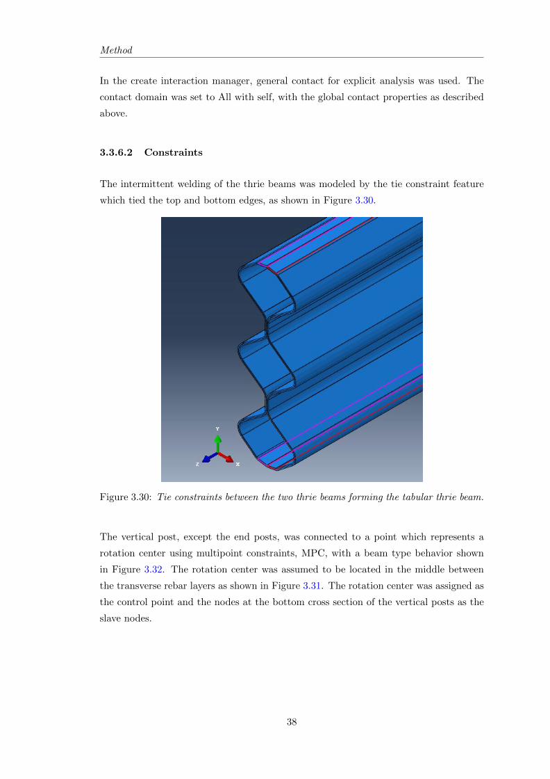
The intermittent welding of the thrie beams was modeled by the tie constraint feature
which tied the top and bottom edges, as shown in Figure 3.30.
Figure 3.30: Tie constraints between the two thrie beams forming the tabular thrie beam.
The vertical post, except the end posts, was connected to a point which represents a
rotation center using multipoint constraints, MPC, with a beam type behavior shown
in Figure 3.32. The rotation center was assumed to be located in the middle between
the transverse rebar layers as shown in Figure 3.31. The rotation center was assigned as
the control point and the nodes at the bottom cross section of the vertical posts as the
slave nodes.
38

Method
Figure 3.31: Rotation center in the bridge deck.
Figure 3.32: The constraints between the vertical posts and the rotational center.
3.3.6.3 Connections
Attachment points were created for the thrie beam at the location where the bolt con-
nections to the vertical posts were located. This was done to fasten the two thrie beams
together using fasteners in the Engineering features of the assembly module. The phys-
ical radius was set to 7.9375 mm and a beam connector section was assigned to the
fasteners. The neglected bolts connecting the tabular thrie beam and the vertical posts
were modeled by creating wires that was assigned a Cartesian connector section, see
Figure 3.33. The properties used for the connector section is tabulated in Table 3.6.
39

Method
Figure 3.33: The connection between the tabular thrie beam and vertical post.
Table 3.6: Properties of the Cartesian connector section.
Nonlinear elasticity F1 [N] U [mm] F2 and F3 [N] U [mm]
-36000 -56 -79200 -15
0 0 0 0
36000 56 79200 15
Failure U1 [mm] U2 and U3 [mm]
Upper bound -150 -50
Lower bound 150 50
The values of the forces in Table 3.6 were based on Appendix A.1. A parametric study
was made for di↵erent values of the corresponding displacements until the behavior of
the bolt connection partially converged to the full-scale test. Same principles were used
for the displacement of the failure.
A rigid Cartesian connection was used for the bolts connecting the tabular thrie beam
and the end posts. The usage of this type of connection was based on that neither
translation nor rotations were present at these points of the tabular thrie beam in the
full-scale test.
40

Method
The rotation center, RC, shown in Figure 3.31 was assigned the wire-to-ground feature.
The wire-to-ground was assigned a Cartesian+Rotation connector section with prop-
erties according to Table 3.7. Five of the constrained components of relative motion,
CORM, were set to rigid. The only CORM that was assigned properties was M3, which
was rotation about the z-axis in the model. The coupling definition was set to uncou-
pled, the regularization tolerance in the table option of the connector section was set to
the default value while the extrapolation was set to linear. This procedure was applied
to all vertical posts except the two end posts.
The rotational sti↵ness between the connecting post and bridge deck was di�cult to
predict. However, it could be recognized that the posts did not buckle in the full-scale
test which indicated that the rotational sti↵ness of the connection must be less than the
yielding moment of posts. Hand calculations were made to estimate the maximum mo-
ment capacity of the vertical post, see Appendix A.2. A simulation was also performed
for fully fixed bottom of the posts to determine the maximum rotational moment, which
was 5.5E6 Nmm. A parametric study was made for di↵erent values of the rotational mo-
ment ranging from 1E6 to 21E6 Nmm, until the rotational moment gave approximately
similar angular displacements as in the full-scale test.
Table 3.7: Properties of the Cartesian+Rotation connector section.
Nonlinear elasticity M3 [Nmm] UR3 [Rad]
-5E6 -0.0001
0 0
5E6 0.0001
Nonlinear plasticity M3 [Nmm] UR3 [Rad]
5E6 0
18E6 0.79
1 2
41

Method
3.3.7 Load
Gravity load with a value of 9810 mm/s2 was applied for the entire vehicle.
Impact velocity of the vehicle was, 27761 mm/s (62.1 mi/h). The velocity was applied
through the predefined field feature. V1-component and V3-component was set to 11202
mm/s and -25401 mm/s respectively, giving a resultant of 27761 mm/s.
3.3.8 Boundary conditions
The rigid bridge deck was assigned a reference point at the middle where fixed, ENCAS-
TRE, boundary condition was applied.
Fixed boundary conditions, ENCASTRE, were applied to the bottom of the two end
posts, see Figure 3.34. The usage of this type of boundary condition was based on that
neither translation nor rotations were present at these points in the full-scale test.
Figure 3.34: The fixed boundary condition applied to the end post.
42

Method
3.3.8.1 Summary of the assumptions and simplifications
The assumptions and simplifications used in the finite element modeling, excluding the
vehicle model, are summarized in this section by the listed bullets below.
• Transition zones of the test installation were not included in the FE-modeling.
• The bridge deck was not modeled as in the full-scale test, instead a rigid solid
element was used.
• Base plate between the bridge deck and the posts were not modeled.
• Plastic o↵set block between the tabular thrie beam and vertical posts were ex-
cluded from the model.
• Intermittent welds of the tabular thrie beam were not modeled, instead the top
and bottom edges of the thrie beams were tied together.
• Slotted holes and bolts in the tabular thrie beam and vertical post were not con-
sidered.
43

Chapter 4
Results
In this chapter the results of interest are presented. The chapter starts out with a brief
presentation of the results from full-scale crash test perform by Texas Transportation
Institute followed by a section where simulation results are presented. At the end of this
chapter a qualitative and quantitative comparison between the results of the full-scale
test and simulation is performed.
4.1 Results of the full-scale crash test
Results that are presented here are brief and mostly qualitative in order to compare them
with the results from the simulation. The reader should read through [2] if interested in
results such as occupant risks and other results of importance.
Approximately at 0.027 s after the impact, post 11 started to deflect to the side of the
field. Post 12 and 13 deflected to the side of the field at 0.061 s and 0.068 s respectively.
After impacting the bridge rail, the vehicle started to travel parallel with the bridge
rail at 0.259 s with a speed of 48.1 mi/h (approx. 77.4 km/h). At 0.267 s the vehicle
began to roll and continued to roll as it exited the view of the overhead camera. The
vehicle came to rest on its right side 163 ft. (approx. 49.7 m) downstream of the impact
point and 48 ft. (approx. 14.6m) from the tra�c face of the rail as shown in Figure 4.4.
Sequential photographs are shown Figure 4.1 to Figure 4.3.
44

Results
Figure 4.1: Sequential photographs of the test, overhead and frontal view [2].
45

Results
Figure 4.2: Sequential photographs of the test, overhead and frontal view (continued)[2].
46

Results
(a) 0 s (b) 0.086 s
(c) 0.169 s (d) 0.255 s
(e) 0.341 s (f) 0.427 s
(g) 0.511 s (h) 0.597 s
Figure 4.3: Rear view of the crash[2].
47

Results
Figure 4.4: The impact point and end point of the vehicle[2].
4.1.1 Damage to the test installation
Measurements of the modified T8 bridge rail showed that the installation did not work
as intended. Post 5 through 9 rotated clockwise with an angle of 5 degrees[2]. Failure
mechanism was crushing of the concrete deck as shown in Figure 4.5. Post 10 through
15 experienced the largest deformations, the deformation for these posts are listed in
Table 4.1.
Table 4.1: Post deformation and deflection[2].
Post
No.
Lean Toward
Field Side [°]Deflection Toward
Field Side [in]
10 10 1.5 (38mm)
11 35 5.25 (133 mm)
12 58 8.5 (210 mm)
13 120 14.25 (362 mm)
14 17 3.125 (79 mm)
15 5 0.625 (16 mm)
Post-to-rail connection bolt pulled through the thrie beam at post 11 through 13 and the
first layer of the thrie beam element at post 14. The vehicle was in contact with the rail
a distance of 24.75 ft. (approx. 7.54 m). Dynamic deflection of the bridge rail during
the impact was 1.91 ft. (approx. 582 mm) and the maximum permanent deformation
was 1.69 ft. (approx. 515 mm), deformations can be seen in Figure 4.6.
48

Results
Figure 4.5: Damage to the test installation[2].
49

Results
Figure 4.6: Permanent deformation to the test installation[2].
50

Results
4.1.2 Damage to the test vehicle
Damages to the vehicle can be seen in Figure 4.7. Maximum exterior crushing was
about 13.0 inches (330 mm) in the front plane at the left front corner at bumper height.
Damage was also present for the front bumper, hood, grill, left front fender, left tire and
wheel rim, left door, and left rear exterior bed[2]. The windshield and door glass broke
when the vehicle rolled onto its side, also visible in Figure 4.7.
Figure 4.7: Vehicle after being up-righted [2].
4.2 Results of the simulation
Only key values from the simulated crash are presented here, more details regarding the
results are presented in Appendix B.
Approximately at 0.017 s after the impact, post 11 started to deflect to the field side.
Post 12 and 13 deflected to the side of the field at 0.019 s and 0.034 s respectively. After
impacting the bridge rail, the modeled vehicle started to travel parallel (it had rotated
with an angle of 23.8°) with the modeled bridge rail at 0.213 s with a speed of 85.1 km/h.
Time for when the vehicle started to roll was not clear, however the rolling motion was
present somewhere between 0.200 s and 0.255 s. The simulation was terminated after 0.6
s since all the sequential photographs needed were obtained at this time step. Total time
51

Results
of the analysis was approximately 34 h. Sequential photographs from the simulation are
shown in Figure 4.8 to Figure 4.10.
(a) 0 s (b) 0 s
(c) 0.086 s (d) 0.086 s
(e) 0.169 s (f) 0.169 s
(g) 0.255 s (h) 0.255 s
Figure 4.8: Sequential simulations photographs - top and front view.
52

Results
(a) 0.341 s (b) 0.341 s
(c) 0.427 s (d) 0.427 s
(e) 0.511 s (f) 0.511 s
(g) 0.597 s (h) 0.597 s
Figure 4.9: Sequential simulations photographs - top and front view (continued).
53

Results
(a) 0.000 s (b) 0.086 s
(c) 0.169 s (d) 0.255 s
(e) 0.341 s (f) 0.427 s
(g) 0.511 s (h) 0.597 s
Figure 4.10: Sequential simulations photographs - rear view.
54

Results
4.2.1 Damage to the modeled installation
Post 5 through 9 rotated clockwise with a mean angle of 3.3°. Post 10 through 15
experienced the largest deformation, the deformation for these posts are tabulated in
Table 4.2.
Table 4.2: Post deformation and deflection in the simulation.
Post
No.
Lean Toward
Field Side [°]Deflection Toward
Field Side [mm]
10 17 40
11 31 121
12 51 321
13 51 311
14 35 155
15 20 53
Post-to-rail connector section was detached from the thrie beam at post 13. The vehicle
was in contact with the rail a distance of 7.04 m. Dynamic deflection of the bridge rail
during the impact was 703 mm and the maximum permanent deformation was 643 mm,
deformations can be seen in the following figures.
Figure 4.11: Deflection of the posts which experienced the largest deformations.
55

Results
Figure 4.12: Damage to the modeled installation - front view.
Figure 4.13: Damage to the modeled installation - rear view.
56

Results
4.2.2 Damage to the modeled vehicle
The exterior damages to the modeled vehicle are shown in Figure 4.14, however it should
be noticed that these deformations were present at a time of 0.6 s which is not when the
vehicle came to rest. Maximum exterior crushing was about 297 mm in the front plane
at the left front corner at bumper height. Non blue color in Figure 4.14 represents other
damages to the vehicle. It should be noticed that the tires were elastically defined and
will not have permanent damages.
Figure 4.14: Damage to the vehicle at 0.6 s.
57

Results
4.2.3 Energy quantities
Di↵erent energy quantities from the simulation are presented below. The kinetic energy
for the modeled vehicle was calculated by hand using equation 4.1,
Ekinetic =mv2
2. (4.1)
with values inserted, the kinetic energy of the modeled vehicle was calculated to 776.1 kJ.
This value was also obtained from Abaqus for the EKE and Etotal at the very beginning
of the simulation as can be seen in Figure 4.15.
0 0.05 0.1 0.15 0.2 0.25 0.3 0.35 0.4 0.45 0.5 0.55 0.6 0.65 0.7�200
0
200
400
600
800
1,000
Time t [s]
Energy
[kJ]
Energy quantities for the whole model
E
A
E
CD
E
DMD
E
W
E
FD
E
I
E
KE
E
P
E
E
E
total
E
V
Figure 4.15: Energy quantities for the whole model.
As mentioned in section 2.5, the total energy should be constant during the analysis,
however this was not the case during the simulation. The energy that was contributing
the most to the increase in total energy was the dissipated viscous energy, EV . The
di↵erence in total energy with and without EV is shown in Figure 4.16. The di↵erence
in total energy during the simulation was calculated as,
diff =
✓Etotal
Etotal.initial� 1
◆⇥ 100. (4.2)
It is clear that without increase in EV , the total energy is almost constant with a
maximum deviation of 3.2 %. The reason for the increase in EV is discussed in Chapter
5.
58

Results
0 0.05 0.1 0.15 0.2 0.25 0.3 0.35 0.4 0.45 0.5 0.55 0.6 0.65 0.7�5
0
5
10
15
20
25
30
3.2872
24.8751
Time t [s]
Di↵erence
inE
total[%
]
Etotal during the simulation
E
total
without E
V
E
total
Figure 4.16: Di↵erence in the total energy for the whole model.
4.3 Qualitative comparisons
This section serves as the qualitative comparison between the full-scale crash test and
the simulated crash. Below a comparison on the vehicle behavior and the parapet during
the impact are presented through sequential photographs from di↵erent angles.
No specific values are presented in this section, the comparison in di↵erent key values
are to be found in the quantitative section 4.4.
59

Results
(a) 0 s (b) 0 s
(c) 0.086 s (d) 0.086 s
(e) 0.169 s (f) 0.169 s
(g) 0.255 s (h) 0.255 s
Figure 4.17: Sequential crash photographs comparison - front view.
60

Results
(a) 0.341 s (b) 0.341 s
(c) 0.427 s (d) 0.427 s
(e) 0.511 s (f) 0.511 s
(g) 0.597 s (h) 0.597 s
Figure 4.18: Sequential crash photographs comparison - front view (continued).
61

Results
(a) 0 s (b) 0 s
(c) 0.086 s (d) 0.086 s
(e) 0.169 s (f) 0.169 s
(g) 0.255 s (h) 0.255 s
Figure 4.19: Sequential crash photographs comparison - top view.
62

Results
(a) 0.341 s (b) 0.341 s
(c) 0.427 s (d) 0.427 s
(e) 0.511 s (f) 0.511 s
(g) 0.597 s (h) 0.597 s
Figure 4.20: Sequential crash photographs comparison - top view (continued).
63

Results
(a) 0 s (b) 0 s
(c) 0.086 s (d) 0.086 s
(e) 0.169 s (f) 0.169 s
(g) 0.255 s (h) 0.255 s
Figure 4.21: Sequential crash photographs comparison - rear view.
64

Results
(a) 0.341 s (b) 0.341 s
(c) 0.427 s (d) 0.427 s
(e) 0.511 s (f) 0.511 s
(g) 0.597 s (h) 0.597 s
Figure 4.22: Sequential crash photographs comparison - rear view (continued).
65

Results
4.4 Quantitative comparisons
To determine the accuracy of the simulated crash in replicating the full-scale crash test,
key parameters obtained from the simulation were compared to those of the full-scale
crash test.
At 0.027 s after impact, post 11 started to deflect in the full-scale test compared to 0.017
s from the simulation. Post 12 and 13 deflected at 0.061 s and 0.068 s compared to 0.019
s and 0.034 s.
After impacting the bridge rail, the test vehicle started to travel parallel with the bridge
rail at 0.259 s with a speed of 77.4 km/h corresponding values from the simulation were
0.213 s with a speed of 85.1 km/h. At 0.267 s the test vehicle started to roll. It was
di�cult to determine the time for the initiation of the rolling motion in the simulations,
however somewhere between 0.200 s and 0.255 s.
Dynamic deflection and permanent deformation of the bridge rail during the test was
582 mm respectively 515 mm compared to 703 mm and 643 mm from the simulation.
The comparison in post deflections and deformation between full-scale test and simula-
tion are tabulated in Table 4.3 and Table 4.4.
Table 4.3: Post angular deflection - comparison.
Simulation Full-scale �
Post
No.
Lean Toward Field
Side [°]Lean Toward Field
Side [°][°]
10 17 10 7
11 31 35 4
12 51 58 7
13 51 120 Not Comparable
14 35 17 18
15 20 5 15
66
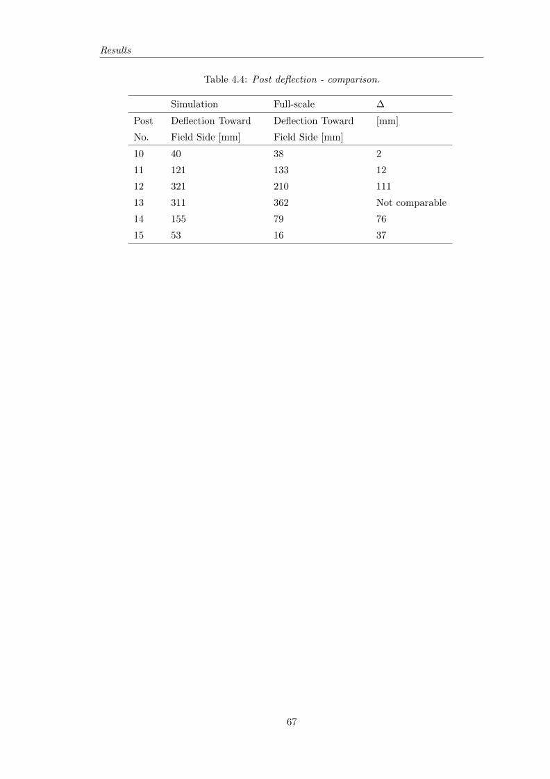
Results
Table 4.4: Post deflection - comparison.
Simulation Full-scale �
Post
No.
Deflection Toward
Field Side [mm]
Deflection Toward
Field Side [mm]
[mm]
10 40 38 2
11 121 133 12
12 321 210 111
13 311 362 Not comparable
14 155 79 76
15 53 16 37
67

Chapter 5
Discussion and conclusions
As can be seen from the comparison sections in the previous chapter, there are similarities
and di↵erences between simulation and full-scale test results. In this chapter some of
the results are discussed and analyzed in order to draw any conclusions.
Results of the simulation showed that post 11 through 13 deflected earlier than the
performed full-scale test. One reason for this could be that the elastic definition of the
applied rotational sti↵ness was not large enough. It was burdensome to predict the sti↵-
ness of the neglected concrete bridge deck. Another reason could be the sti↵ness of the
neglected transition zone which was not captured by the applied boundary conditions.
The neglected o↵set block could also contribute to early deflection of these posts, we
believe that the o↵set block absorbs a portion of the impulse created initially by the
impact and thus deforms plastically which delays the deflection of vertical posts. This
means that the impulse stress applied to the posts in the test was smaller than in the
simulation.
Post deflections were fairly accurate for posts 5 through 12. The collapse of post 13 was
not captured by only using rotational sti↵ness as the failure mechanism between the
concrete bridge deck and vertical post. Deflection for post 14 and 15 was also slightly
di↵erent compared to the full-scale test. A reason for this could be that the loss in vehicle
speed during impact was lower than the full-scale test due to the low friction used in the
model. This provided more energy to deform these posts giving larger deformations.
Bolt-to-rail connection used in the simulation worked as intended only for post 13,
indicating that the real behavior could not be captured to the fullest. It was problematic
to find corresponding values matching the bolts used in the full-scale test.
The low friction applied for the model might be the reason why the vehicle was travelling
parallel with the guardrail at an earlier time step than it actually does in the full-scale
68

Discussion and conclusion
test. The energy losses due to friction were minimal causing the vehicle to travel with a
higher speed.
Deflections obtained for the tabular thrie beam was larger than corresponding values
for the full-scale test. The boundary conditions used in the model did not capture the
sti↵ness provided by the transition zone in the full-scale test. Another reason for the
larger deflections obtained in the simulation could be the larger kinetic energy during
impact as mentioned above. Since the simulation has larger kinetic energy during impact
it will also provide larger plastic deformations.
Sequential comparison showed that the behavior of the simulation was fairly accurate
until the sequence at 0.427 s, after this moment the simulation di↵ers. An explanation
for this could be that the rear of the modeled vehicle did not travel in the same path
as in the full-scale test vehicle. The tabular thrie beam was deflected downwards when
impacted by the front of the car in the full-scale test. It was obvious that the bridge deck
was crushed when the front of the car impacted the parapet meaning that the sti↵ness
provided by the vertical post at the impact area was significantly reduced. There was
only the sti↵ness of tabular thrie beam at this area when the rear of the car impacted
the parapet. The post rotation lowered the height of the thrie beam, causing it to
deflect beneath the rear of the car which caused it to roll onto it right side as it exited
the test installation. This behavior was not accurately reflected in the simulation, the
post rotation did not lower the height of tabular thrie beam to same extent as the full-
scale test. Post 13 provided sti↵ness since it did not collapse as the full-scale test. The
combination of a higher tabular thrie beam together with the sti↵ness provided from
post 13 when impacted by the rear of the modeled vehicle is believed to be the cause of
the di↵erence between the simulation and full-scale test.
Another cause which may influence the rolling motion of vehicle could be the di↵erence
in the center of gravity between the modeled vehicle and tested car. As mentioned in
section 3.3.1.2 there was a di↵erence of approximately 40 mm in the vertical height.
However it was not easy to determine if this di↵erence influenced the behavior of the
modeled vehicle compared to the test vehicle. It is a necessity to model every part of
the parapet and bridge deck in detail in order to study if this di↵erence does influence
the behavior of the modeled vehicle.
Main focus of the master thesis has been to validate the simulation against the full-scale
test. However, another way of validating the model was to briefly study the energy
balance of the simulation. The study of energy balance showed that the total energy
during the simulation was not constant, as it should be. As presented in the result
chapter, the total energy was increased during the simulation. After investigating the
cause of the increase in total energy it was discovered that it was due to the increase
69

Discussion and conclusion
in dissipated viscous energy. This gain of viscous energy was due to the dashpot-like
damping behavior defined for connector sections used to connect adjacent parts in the
engine of the modeled vehicle. Some of these damping factors were very high, when
these parts are in motion the damping will create great amount of dissipated viscous
energy. It can be seen from Figure 4.15 that the dissipated viscous energy continues to
grow at 0.6 s where the vehicle started to land on the floor meaning that large motions
for di↵erent parts of the engine were present which was damped by these dashpot-like
dampers. If these dashpot-like damping factors were not used, it would probably reduce
the increase in viscous dissipated energy since no material damping was used except the
default bulk viscosity introduced by Abaqus. It could also be seen that the total energy
for the whole model was almost constant if the viscous dissipated energy was subtracted
from the total energy.
Artificial strain energy was also studied in order to determine if it was necessary to use
a denser mesh. Several simulation was performed with di↵erent mesh sizes, the mesh
sizes mentioned in the method section were the final ones which reduced the artificial
strain energy to the levels plotted in Figure 4.15. Denser mesh would probably decrease
the artificial strain energy a bit further, however it was not a necessity to decrease the
mesh further since the computational e↵ort would have increased more than what the
gain would be.
Kinetic energy was decreased while the plastic strain energy was increased during the
impact as it should be since the loss in kinetic energy is proportional to the dissipated
energy due to plasticity. This indicated that the model behaved properly.
The conclusion of this master thesis is that Abaqus/Explicit has all the potentials needed
to simulate vehicle crashes. The global sti↵ness of the test installation was not fully
captured by the model used here which provided di↵erence in the results between the
simulation and full-scale test. However, this master thesis shows that a full-scale crash
can be simulated using Abaqus/Explicit provided a proper vehicle model and a detailed
model of the test installation. Nonetheless, it is a prerequisite to model the parapet
and the surroundings such as bridge deck, connections etc. very detailed to have better
convergence with real test. Detailing of the model sets the limit for how accurate the
simulations will be.
70

Chapter 6
Future work
The main area of improvement seems to be the model of the bridge deck and the detailing
in the connection between di↵erent parts of the bridge parapet. In order to produce
better convergence between the simulation and the full-scale test, the overall sti↵ness of
the bridge rail installation must be captured. It is very di�cult to capture the overall
sti↵ness when neglecting key object such as the transition zones, the bolts and the
crushing process of the bridge deck.
A future work could for example be to use the modeled vehicle in this master thesis
and focus on the modeling of the concrete deck and the bridge rail installation. Special
intention should also be addressed for the material definition of the concrete deck since
crushing is involved.
Next step is to improve the material definitions of some parts of the modeled vehicle.
One of these materials could for example be the material definition used for the tires.
Instead of the elastic definition as it is now, it should be modeled with a proper material
definition for rubber. Also, it is necessary to investigate the occupant risks during the
impact. Another property that might be of importance to address is how the vehicle
speed is applied prior impact. The speed of the vehicle is applied through the predefined
field, a more sophisticated way of applying the vehicle speed should be used in order to
reflect the real behavior prior, during and after the impact. In order to get rid of the
increasing viscous dissipated energy, future worker should reconsider the usage of the
dashpot-like properties used for the di↵erent connection sections in the vehicle model.
Attention should be put on the energy balance to have constant total energy for the
whole model.
Looking even further into the future it would be a necessity to develop di↵erent vehicle
models that can be used in the simulations in order to investigate the performance of
71

Future work
the rail. This is a necessity since satisfactory performance of the parapet for a specific
vehicle does not imply the satisfaction for a di↵erent type of vehicle since the overall
sti↵ness must fit di↵erent types of vehicle models as mentioned in the introduction of
this master thesis.
72
Bibliography
[1] Dassault Systemes. Abaqus 6.14 Online Documentation: 2.4.2 Cost of mesh refine-
ment in implicit and explicit analyses. Dassault Systemes, http://server-ifb147.
ethz.ch:2080/v6.14/books/gsa/default.htm, 2014.
[2] Roger P. Bligh, William F. Williams, and Wanda L. Menges. NCHRP REPORT
350 TEST 3-11 OF THE MODIFIED T8 BRIDGE RAIL. Technical report,
Texas Transportation Institute, http://d2dtl5nnlpfr0r.cloudfront.net/tti.
tamu.edu/documents/0-5210-6.pdf, 2009.
[3] Ali O. Atahan and Omer F. Cansiz. Impact analysis of a vertical flared back bridge
rail-to-guardrail transition structure using simulation. http://citeseerx.ist.
psu.edu/viewdoc/download?doi=10.1.1.208.872&rep=rep1&type=pdf, 2004.
[4] National Crash Analysis Center. http: // www. ncac. gwu. edu/ vml/ models.
html , 2014.
[5] Nauman M. Sheikh, Rubiat Ferdous, Roger P. Bligh, and Akram Y. Abu-
Odeh. ANALYSIS OF ROADSIDE SAFETY DEVICES FOR USE ON
VERY HIGH-SPEED ROADWAYS. Technical report, Texas Transportation
Institute, http://d2dtl5nnlpfr0r.cloudfront.net/tti.tamu.edu/documents/
0-6071-1.pdf, 2009.
[6] Nauman M. Sheikh, Rubiat Ferdous, Roger P. Bligh, and Akram Y. Abu-
Odeh. ANALYSIS OF ROADSIDE SAFETY DEVICES FOR USE ON
VERY HIGH-SPEED ROADWAYS. Technical report, Texas Transportation
Institute, http://d2dtl5nnlpfr0r.cloudfront.net/tti.tamu.edu/documents/
0-6071-1.pdf, 2009. p. 14.
[7] Touraj Gholami, Jurgen Lescheticky, and Ralf Paßmann. Crashworthiness simula-
tion of automobiles with abaqus/explicit. 2002.
[8] Xavier Latorre, Pedro Marijuan, and Jordi Vinas. Road restraint systems in abaqus.
2012.
73

Bibliography
[9] Dassault Systemes. Abaqus 6.14 Online Documentation: 1.1 The Abaqus prod-
ucts. Dassault Systemes, http://server-ifb147.ethz.ch:2080/v6.14/books/
gsa/default.htm, 2014.
[10] Dassault Systemes. Abaqus 6.14 Online Documentation: 9.2.1 Explicit time in-
tegration. Dassault Systemes, http://abaqus.sys.kth.se/v6.14/books/gsa/
default.htm, 2014.
[11] Dassault Systemes. Abaqus 6.14 Online Documentation: 2.4.1 Choosing between
implicit and explicit analysis. Dassault Systemes, http://server-ifb147.ethz.
ch:2080/v6.14/books/gsa/default.htm, 2014.
[12] Dassault Systemes. Abaqus 6.14 Online Documentation: 9.2.3 Advantages of the
explicit time integration method. Dassault Systemes, http://abaqus.sys.kth.se/
v6.14/books/gsa/default.htm, 2014.
[13] Dassault Systemes. Abaqus 6.14 Online Documentation: 9.3.1 Conditional stability
of the explicit method. Dassault Systemes, http://abaqus.sys.kth.se/v6.14/
books/gsa/default.htm, 2014.
[14] Dassault Systemes. Abaqus 6.14 Online Documentation: 9.3.2 Definition of the sta-
bility limit. Dassault Systemes, http://abaqus.sys.kth.se/v6.14/books/gsa/
default.htm, 2014.
[15] Dassault Systemes. Abaqus 6.14 Online Documentation: 9.3.3 Fully automatic
time incrementation versus fixed time incrementation in Abaqus/Explicit. Dassault
Systemes, http://abaqus.sys.kth.se/v6.14/books/gsa/default.htm, 2014.
[16] Dassault Systemes. Abaqus 6.14 Online Documentation: 9.3.4 Mass scaling to
control time incrementation. Dassault Systemes, http://abaqus.sys.kth.se/v6.
14/books/gsa/default.htm, 2014.
[17] Dassault Systemes. Abaqus 6.14 Online Documentation: 9.6.1 Statement of en-
ergy balance. Dassault Systemes, http://abaqus.sys.kth.se/v6.14/books/gsa/
default.htm, 2014.
[18] Dassault Systemes. Abaqus 6.14 Online Documentation: 3.2.2 Substructure analysis
of a pick-up truck model. Dassault Systemes, http://server-ifb147.ethz.ch:
2080/v6.14/books/exa/default.htm, 2014.
[19] Dassault Systemes. Abaqus 6.14 Online Documentation: 3.2.1 Inertia relief in a
pick-up truck. Dassault Systemes, http://server-ifb147.ethz.ch:2080/v6.14/
books/exa/default.htm, 2014.
74

Appendix A
A.1 Bolt connection properties
75

Bolt capacity
Indata
tthriebeam 5mm� d58in 15.875mm� � Abolt
π d2�
4197.933mm2� �
Pbolt π d� 49.873mm� � fyb 640MPa� Assuming 8.8 Bolts
γM1 1.0� fub 800MPa�
γM2 1.2� fy.thriebeam 250MPa�
k2 0.9�
αv 0.6�
Tension resistance of the bolts [EN 1993-1-8]
Ft.Rdk2 fub� Abolt�
γM2118.76kN� �
Punching shear resistance of thrie beam [EN 1993-1-1]
PRd Pbolt tthriebeam�fy.thriebeam
3 γM1�� 35.993kN� �
F1 min Ft.Rd PRd��� � 35.993kN� �
Shear resistance of the bolts [EN 1993-1-8]
Fv.Rdαv fub� Abolt�
γM279.173kN� �
F2 Fv.Rd 79.173kN� �
F3 F3=

Bibliography
A.2 Bending moment capacity of the post
77

Post Cross Section: without slotted holes
Indata
bc 3.94in 100.076mm� � tc 0.194in 4.928mm� � fy 250MPa� ε 235fy
MPa
0.97 �
h 5.83in 148.082mm� �
hw h 2tc� 138.227mm� � tw 0.17in 4.318mm� �
Classification of the cross sectionFlange
bc tw�
2 tc�9.716
compare with 9ε10ε14ε
§¨¨©
·¸¸¹
8.726
9.695
13.574
§¨¨©
·¸¸¹
Crosssection 3
Web
hwtw
32.012 compare with
72ε83ε124ε
§¨¨©
·¸¸¹
69.807
80.471
120.222
§¨¨©
·¸¸¹
CrossSection 3
The cross section belongs to Class 3
Moment of inertia
Iy 2bc tc
3�
12bc tc�
h2
§©
·¹
2��
ª««¬
º»»¼
�tw hw
3�
12� 6.359 106u mm4� �
Wy.elIy0.5 h�
8.589 104u mm3� �
Mmax fy Wy.el� 21.472MN mm�� �

Appendix B
B.1 Post deformations
B.1.1 Initial angular deflection of posts 11-13
The time for the initial deflection was set to a value when the deflection was at least 1�
in order to compare to the full-scale test.
0 0.005 0.01 0.015 0.02 0.025 0.03 0.035 0.04 0.045 0.05�20
�15
�10
�5
0
5
10
0.0171430.018858 0.034286
Time t [s]
Angu
lardisplacements
UR3[D
egrees]
Angular deflection, UR3, of post 11-13
Post11
Post12
Post13
Figure B.1: Initial angular deflection of post 11-13.
79

Bibliography
B.1.2 Mean angular deflection for posts 5-9
0 0.05 0.1 0.15 0.2 0.25 0.3 0.35 0.4 0.45 0.5 0.55 0.6 0.65�5
�4
�3
�2
�1
0
1
-3.2959
Time t [s]
Angu
lardisplacements,UR3[°]
Mean values of angular deflection, UR3, for post 5-9
Angular displacement UR3
Figure B.2: Mean angular deflection for posts 5-9.
B.1.3 Angular deflection for posts 10-15
0 0.05 0.1 0.15 0.2 0.25 0.3 0.35 0.4 0.45 0.5 0.55 0.6 0.65 0.7�60
�50
�40
�30
�20
�10
0
10
-17.4037
-30.7955
-51.2094
-50.8964
-34.9414
-20.1809
Time t [s]
Angu
lardisplacements,UR3[°]
Angular deflection, UR3, for posts 10-15
Post10
Post11
Post12
Post13
Post14
Post15
Figure B.3: Angular deflection for posts 10-15.
80

Bibliography
B.1.4 Vertical deflection for posts 10-15
0 0.05 0.1 0.15 0.2 0.25 0.3 0.35 0.4 0.45 0.5 0.55 0.6 0.65 0.7�400
�300
�200
�100
0
100
-39.6246
-121.388
-320.676
-310.779
-154.51
-53.2293
Time t [s]
Verticaldisplacements,U2[m
m]
Deflection towards field side, U2, for posts 10-15
Post10
Post11
Post12
Post13
Post14
Post15
Figure B.4: Deflection towards field side, U2, for posts 10-15.
B.2 Tabular thrie beam deformations
0 0.05 0.1 0.15 0.2 0.25 0.3 0.35 0.4 0.45 0.5 0.55 0.6 0.65 0.7
0
200
400
600
800702.61
642.551
Time t [s]
Horizon
taldisplacements,U1[m
m]
Horizontal deflection, U1, of the tabular thrie beam
Tabular thrie beam deflection
Maximum dynamic deflection
Maximum permanent deformation
Figure B.5: Maximum deflection of the tabular thrie beam.
81

Bibliography
B.3 Vehicle position, speed and angular deflection
When the vehicle had rotated an angle of 23.8°, relative to its initial position, it was
parallel to the bridge guard rail. The graphs and picture presented here shows the
position, speed and time when the vehicle was parallel. The time was 0.213 s when the
car was parallel.
0 0.05 0.1 0.15 0.2 0.25 0.3 0.35 0.4 0.45 0.5 0.55 0.6 0.65 0.7
0
10
20
30
23.8
Time t [s]
Angledefl
ection
,[D
egrees]
Angular deflection of the vehicle
Angle deflection
Angle when parallel to guardrail
Figure B.6: Vehicle angle during the impact.
0 0.05 0.1 0.15 0.2 0.25 0.3 0.35 0.4 0.45 0.5 0.55 0.6 0.65 0.775
80
85
90
95
100
105
85.135
Time t [s]
Speed,V
[km/h
]
Vehicle speed during impact
Resultant of the vehicle speed
Speed at parallel to guardrail
Figure B.7: Vehicle speed during the impact.
82
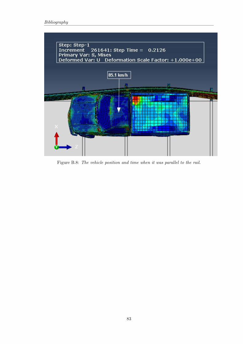
Bibliography
Figure B.8: The vehicle position and time when it was parallel to the rail.
83