IngenIería e InvestIgacIón vol. 37 n.° 3, december - 2017 (92-101)

92

Simulation of unsteady blood flow dynamics in the thoracic aorta

Simulación transitoria de la dinámica del flujo sanguíneo en la aorta torácica

Santiago Laín1, and Andrés D. Caballero2

ABSTRACT

In this work, blood flow dynamics was analyzed in a realistic thoracic aorta (TA) model under unsteady-state conditions via velocity contours, secondary flow, pressure and wall shear stress (WSS) distributions. Our results demonstrated that the primary flow velocity is skewed towards the inner wall of the ascending aorta; but this skewness shifts towards the posterior wall in the aortic arch and then towards the anterior-outer wall in the descending aorta. Within the three arch branches, the flow velocity is skewed to the distal walls with flow reversal along the proximal walls. Strong secondary flow motion is observed in the TA, especially at the inlet of the arch branches. WSS is highly dynamic, but was found to be the lowest along the proximal walls of the arch branches. Finally, pressure was found to be low along the inner aortic wall and in the proximal walls of the arch branches, and high around the three stagnation regions distal to the arch branches and along the outer wall of the ascending aorta.

Keywords: Blood flow, computational fluid dynamics, hemodynamics, thoracic aorta, wall shear stress.

RESUMEN

En este trabajo se analiza la dinámica del flujo sanguíneo en un modelo realista de la aorta torácica (TA, por sus siglas en inglés) en condiciones transitorias visualizando las distribuciones de velocidad, flujo secundario, presión y esfuerzos cortantes parietales (WSS). Los resultados obtenidos muestran que la velocidad primaria del flujo tiende hacia la pared interior de la aorta ascendente, pero esta, a su vez, tiende hacia la pared posterior en el arco aórtico y hacia las paredes anterior y exterior en la aorta descendente. En las tres ramificaciones del arco aórtico la velocidad del flujo se acerca hacia las paredes distales mostrando recirculación del flujo en las cercanías de las paredes proximales. En la TA se observa un flujo secundario intenso, especialmente a la entrada de las ramificaciones del arco. Finalmente, la presión es baja a lo largo de la pared interior de la aorta y en las paredes proximales de las ramificaciones, mientras que es alta en las zonas de estancamiento situadas en las paredes distales de las ramificaciones así como a lo largo de la pared exterior de la aorta ascendente.

Palabras clave: Flujo sanguíneo, dinámica de fluidos computacional, hemodinámica, aorta torácica, esfuerzos cortantes parietales.

Received: August 25th 2016Accepted: August 14th 2017

DOI: http://dx.doi.org/10.15446/ing.investig.v37n3.59761

1 Physicist, Mathematician and Ph.D., Universidad of Zaragoza, Spain. Dr.-Ing., Habil. Martin Luther University Halle-Wittenberg Germany. Affiliation: Fluid Mechanics Professor, Universidad Autónoma de Occidente, Colombia.

1 E-mail: slain@uao.edu.co2 Biomedical Engineer, Universidad Autónoma de Occidente, Colombia. M.Sc.

Georgia Institute of Technology, USA. Affiliation: Tissue Mechanics Laboratory, The Wallace H. Coulter Department of Biomedical Engineering, Georgia Insti-tute of Technology, Technology Enterprise Park, 387 Technology Circle, Atlan-ta, GA 30313-2412, USA. E-mail: adcaballero@gatech.edu.

How to cite: Laín, S., Caballero, A.D. (2017). Simulation of unsteady blood flow dynamics in the thoracic aorta. Ingeniería e Investigación, 37(3), 92-101. DOI: 10.15446/ing.investig.v37n3.59761

Attribution 4.0 International (CC BY 4.0) Share - Adapt

Introduction

It has long been recognized that the forces and stresses produced by the blood flow on the walls of the cardiovascular system are central to the development of different cardiovascular diseases (CVDs). Nowadays, the reason why arterial diseases occur at preferential sites is still not fully understood, but these regions coincide with complex flow dynamics; especially with low and oscillatory wall shear stress (WSS) (Cecchi et al., 2011). Since these lesions tend to localize in regions of complex arterial geometry, such as bends, tapering, and branching, the thoracic aorta (TA) with its complex anatomy has been considered as one of the most susceptible arteries for the initialization of atherosclerosis and other CVDs.

Development of computational fluid dynamics (CFD) in recent years has enabled the use of three-dimensional (3D) numerical simulations to investigate patient-specific hemodynamics and to understand the origin and

development of different CVDs. The highly disturbed flow patterns that have been reported in regions of arterial branching and curvature are attributable mainly to the combined effects of complex arterial geometry and flow pulsatility. Therefore, CFD studies that aim to generate physiologically relevant blood flow information need to be

IngenIería e InvestIgacIón vol. 37 n.° 3, december - 2017 (92-101) 93

LAÍN AND CABALLERO

based on realistic geometries and to incorporate the time-dependent nature of blood flow.

One vascular site within which the fluid mechanical environment is especially complex is the region of the TA with its major branches. For a recent comprehensible review on CFD modelling in human TA we refer to Caballero and Laín (2013).

Usually, at the upstream side of the artery of interest, a velocity boundary condition is prescribed at the inlet, with an idealized profile such as a flat (plug), fully developed (parabolic) or Womersley flow pattern, or based on time-varying velocity data obtained with PC-MRI or ultrasound. Particularly, a flat velocity profile used together with a pulsatile waveform is often the preferred inlet boundary condition in transient TA studies. This pulsatile waveform is generally based on experimental data reported by Pedley (1980), and it is characterized by accelerating, decelerating, reversed, and zero flow regions. The assumption of a flat velocity profile at the aortic inlet has been verified by various in-vivo measurements using hot-film anemometry on different animal models, which have demonstrated that the velocity profile distal to the aortic valve is essentially flat in the ascending aorta, skewed towards the inner wall with respect to the aortic arch and only consisted of a weak helical component (Seed & Wood, 1971).

However, the fact is that the blood flowing into the TA pumped by the left ventricle (LV) exhibits a complex 3D nature. Blood flow patterns in the healthy TA range from axial during the early portion of systole, to helical during mid-to-late systole, and complex flow recirculation during end systole and diastole (Kilner et al., 1993). The development of helical flow patterns during peak to late systole is thought to be produced by several factors: (i) due to the arrangement of the muscle fibers, the LV undergoes a significant torsional deformation, twisting in a counterclockwise direction during systole and then returning in a clockwise direction during diastole, resulting in diastolic recoil; (ii) the opening and closing dynamics of the aortic valve leaflets and their asymmetric configuration; and (iii) the curvature and the non-planarity of the TA. As aortic helical flow is a common feature in normal individuals as the consequence of the natural optimization of fluid transport processes in the cardiovascular system (Morbiducci et al., 2011), and it is strictly related to transport phenomena of oxygen and LDL (Liu et al., 2011), great attention should be put when idealized velocity profiles are applied at the inlet boundaries of TA computational models.

On the other hand, time-varying pressure waveforms, usually available from catheterization based pressure acquisition technologies, are less frequently prescribed as inlet boundary conditions (Park et al., 2007). Although it is claimed that the driving force for the blood flow in an artery is the pulsatile pressure gradient along the artery, the amount of blood flowing in the computational model is very sensitive to pressure gradients between inlet and outlets. As

the pressure differences between these boundaries are only a small percentage of the systolic-diastolic pulse amplitude, this imposes the problem of accurately determine the pressure, a condition that is difficult to reach in practice. Thus, small errors in the imposed pressure data could lead to great departure of the velocities from the actual values. Moreover, patient-specific pressure data is not currently acquired with enough precision to serve this purpose since an invasive approach could introduce sources of error and artefacts such as deterioration in frequency response, catheter whip artefact, end-pressure artefact, and systolic pressure amplification in the periphery, among others (Kern et al., 2009).

In contrast to several developments made in the area of outlet boundary conditions, little progress has been reported for the influence of inlet boundary conditions in CFD studies of large arteries, despite the fact that proximal to the inlet boundary there is also an upstream part of the cardiovascular system that interacts with the computational domain. Morbiducci et al. (Morbiducci et al., 2013) studied how flat and fully developed inlet velocity profiles affect patient-specific simulated hemodynamics in the TA when compared to simulations employing PC-MRI measured 3D and axial (1D) velocity profiles of the patient’s own in-vivo measured flow data. The obtained results were compared in terms of WSS distribution and helical flow structures. It was found that the imposition of PC-MRI measured axial velocity profiles at the inlet may capture disturbed shear with sufficient accuracy, without the need to prescribe (and measure) realistic fully 3D velocity profiles. Likewise, attention should be put in setting idealized or PC-MRI measured axial velocity profiles at the inlet of the TA computational model when transport phenomena are investigated, since helical flow structures are markedly affected by the boundary condition prescribed at the inlet.

In this paper, blood flow dynamics is analyzed in a realistic thoracic aorta (TA) model under transient conditions. Section 2 presents the employed geometry, mesh elaboration, physical models and the numerical set-up. The obtained results for velocity (main stream and secondary flow), pressure and wall shear stress (WSS) fields are introduced and discussed in section 3. Finally, section 4 presents the main conclusions obtained in this work.

Methods

Geometric model and mesh generation

The geometric model of the TA was obtained from the Simtk.org cardiovascular model repository (Simbios Project, 2007) (see Figure 1a and Table 1) and discretized with high quality tetrahedral/prisms cells using ICEM CFD 13.0 (ANSYS Inc,). Five prism layers adjacent to the arterial wall were set to grow exponentially until the volume transition between the prisms and tetras elements was locally optimized (see Figure 1b). In order to assure that the results were mesh

Simulation of unSteady blood flow dynamicS in the thoracic aorta

IngenIería e InvestIgacIón vol. 37 n.° 3, december - 2017 (92-101)94

independent, the dynamic mesh-adaptation refinement technique of FLUENT 13.0 (ANSYS Inc,) was used to obtain a set of four mesh sizes, in which the computed velocity gradient was used to guide the placement of the cells. The circumferential average of the WSS and the velocity profile at the aortic arch entrance and outlet were chosen as quantities for comparison in the mesh independence study (Caballero & Laín, 2015; Prakash & Ethier, 2001). Mesh definition was considered acceptable when no significant difference (lower than 5%) between successive meshes was noticed. Grid independency was achieved for these two criteria with 1728720 cells.

based on experimental data reported by Pedley (1980), and it is characterized by accelerating, decelerating and zero flow regions (see Figure 2). It is noted that flow reversal is not considered in the input waverform. The assumption of a flat velocity profile at the aortic inlet has been verified by various in-vivo measurements using hot-film anemometry on different animal models, which have demonstrated that the velocity profile distal to the aortic valve is essentially flat in the ascending aorta and only contains a weak helical component (Nerem et al., 1974).

Outflow boundary conditions (specified fractions of the inflow) were imposed at the outlets. According to Middleman (1972), approximately 5 % of the flow volume is assumed to leave the TA through each of the three arch branches. These fractions were recalculated based on the outlet area of each branch and we assumed that this flow percentage remained constant during the entire cardiac cycle. The percentages used were 9,5 %, 5 %, 6,5 % and 79 % for the brachiocephalic artery (BA), left common carotid artery (LCA), left subclavian artery (LSA) and descending aorta, respectively.

From a typical cardiac cycle lasting 0,8 s, the blood flow dynamics was analyzed at four time instances: t = 0,170 s (maximum acceleration), t = 0,250 s (maximum velocity), t = 0,330 s (maximum deceleration), and t = 0,450 s (minimum velocity); see Figure 2. The time average input velocity was 0,0811 m/s with a maximum input velocity of 0,2970 m/s. In our study, the corresponding Reynolds number based on the peak systole velocity was Re = 2072 and the Womersley number (Womersley, 1955) was 18. The diameter at the inlet of the TA model was used to calculate both Reynolds and Womersley numbers. Generally, blood flow in large arteries has been assumed to be laminar. For pulsatile flow turbulence may occur for a Reynolds number much larger than expected for steady flow, due to the fact than accelerating flows tend to be more stable than steady flows (Fung, 1997). Since our Reynolds number is below the critical or threshold Reynolds number, the flow in our model was aumed to be laminar.

Numerical modeling

The Navier-Stokes equations governing the fluid motion were solved by the finite volume CFD code FLUENT 13.0 (ANSYS Inc, Cannonsburg, PA, USA). A pressure-based segregated algorithm was chosen as the solver type. Discretization of the equations at each control volume was achieved by the Second-Order Upwind scheme, which uses larger stencils for second order accuracy, essential with hybrid tetrahedral meshes. The SIMPLE algorithm was used for the coupling of the pressure-velocity terms, needed when computing incompressible flows (Versteeg & Malalasekera, 2007), while the PRESTO! scheme was used for the pressure interpolation, as recommended in domains with high curvature. Finally, the unsteady terms were solved by the bounded second order implicit formulation.

Table 1. TA model dimensions (cm)

Aorta

Inlet diameter 2,4

Outlet diameter 1,9

Length 32

BA

Inlet diameter 1,18

Outlet diameter 1,3

Length 3,4

LCA

Inlet diameter 0,8

Outlet diameter 0,7

Length 5

LSA

Inlet diameter 1,2

Outlet diameter 0,85

Length 3,5

Source: Authors

Governing equations

Under the assumptions of an incompressible, homogenous, Newtonian fluid, the Navier-Stokes and continuity equations can be described as:

ρ ∂u∂t

+ ρ u ⋅∇( )u = −∇p + µ∇2u (1)

∇ ⋅u = 0 (2)

where the primary variables are the velocity vector u = [u, v, w ]and the pressure p that vary in space x, y, z and time t.

Boundary conditions

The blood was assumed to be incompressible, homogeneous and Newtonian fluid with a dynamic viscosity of 0,0035 Pa s and a density of 1 060 kg/m3. The arterial wall was considered to be rigid and the no-slip condition was applied. To simulate a cardiac cycle, a time-dependent flat (plug) velocity profile used together with a pulsatile waveform was applied as inlet boundary condition (Dabagh et al., 2015; Morris et al., 2005; Shahcheraghi et al., 2002). This physiologically representative pulsatile waveform is

INGENIERÍA E INVESTIGACIÓN VOL. 37 N.° 3, DECEMBER - 2017 (92-101) 95

LAÍN AND CABALLERO

In order to start the cardiac cycle calculations, a steady state solution was fi rst obtained using the peak systole velocity. Next, this solution was then used as the initial condition for the unsteady calculations which were in turn solved for a certain number of cycles until a time-periodic solution was obtained. The fi fth cardiac cycle was used as the fi nal periodic solution and it is presented in this paper. The time step size was set at 0,001 s and a maximum of 100 iterations were performed per each time step. Simulations were considered to be converged when the residuals of the Navier-Stokes equations were kept at 1 × 10-6 with verifying mass conservation in 0,5 %, and the net imbalance was well below than 1 % of the smallest fl ux through the boundary domain. In addition, pressure and velocity monitors were placed in the arch branches and descending aorta to assess the solution convergence.

Results

Velocity distribution

A very important aspect of the analysis of 3D fl ows in the cardiovascular system is the graphical presentation of the fl ow fi eld. We present the axial fl ow velocity contours at 18 cross-sections of the TA model (see Figure 1a), at the mentioned four time instances of the cardiac cycle: maximum acceleration, maximum velocity, maximum deceleration and minimum (zero) velocity. For the purposes of enhanced visibility we show the results from the view defi ned in Figure 1b, and this view was found to give the best presentation of our results.

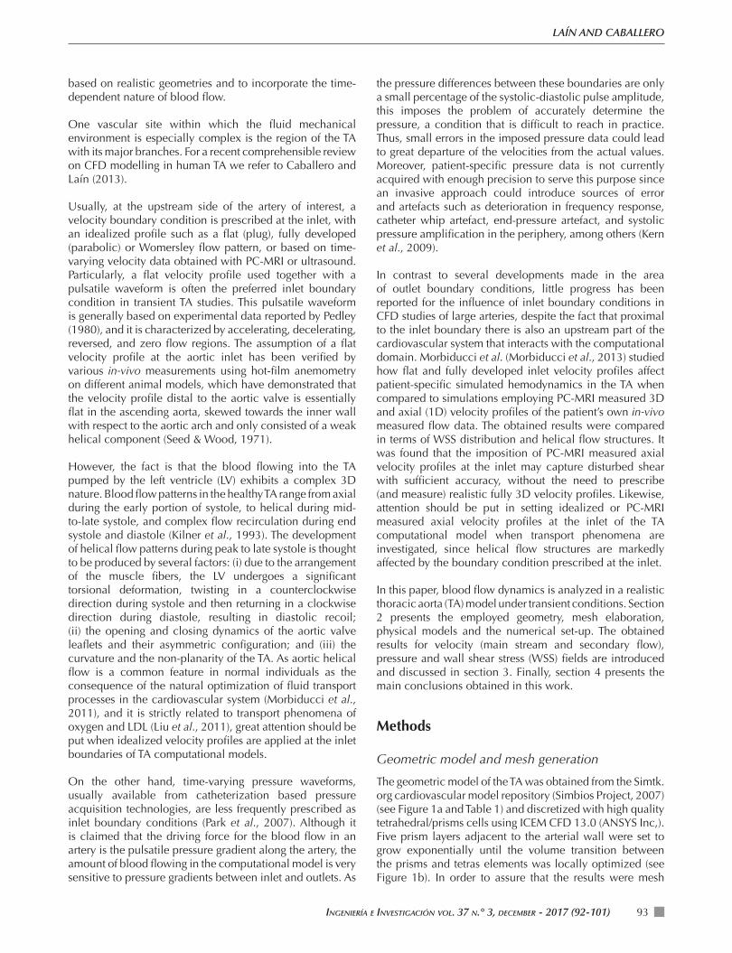
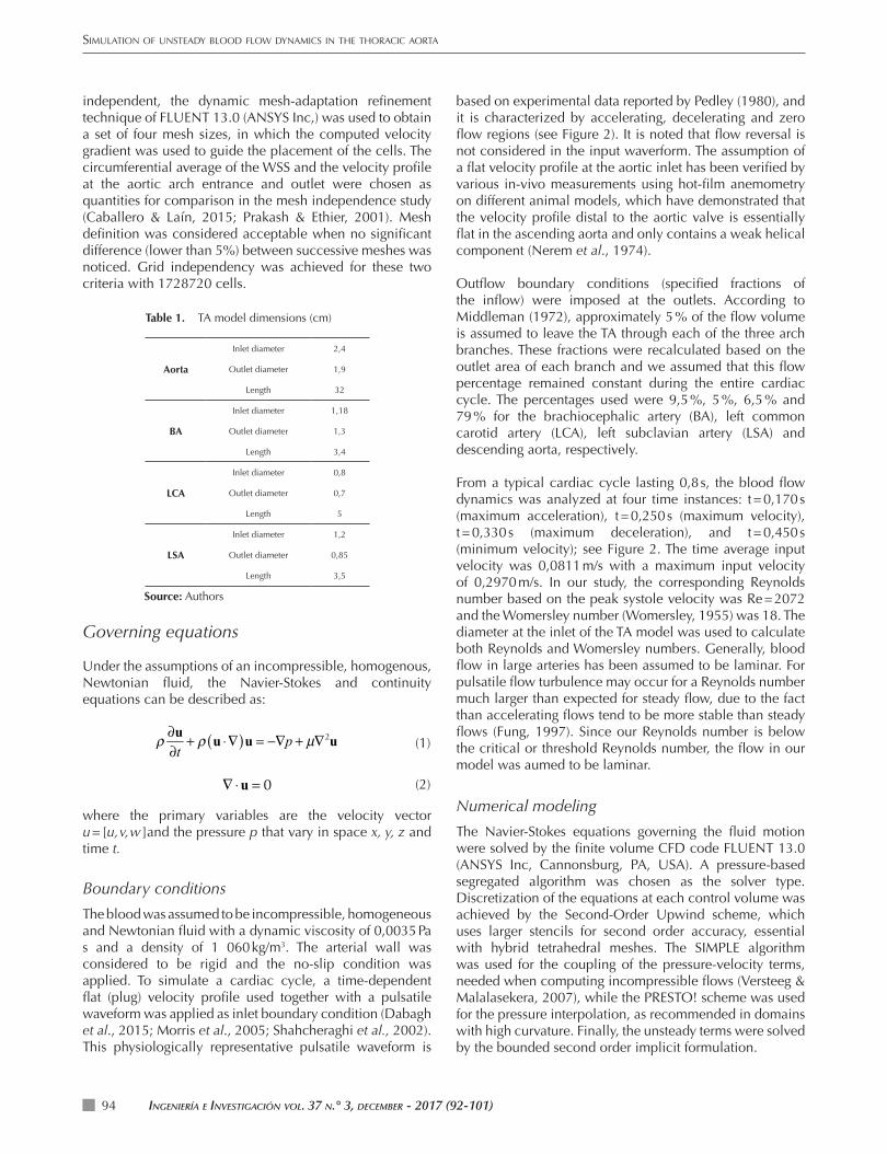
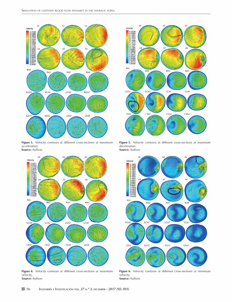
The results demonstrate that for the time points with positive inlet velocity (Figures 3 to 5), the fl ow at the ascending aorta (cross-sections A1 and A2) is consistently skewed towards the inner aortic wall. This vortical type velocity profi le has been induced by the curved entrance geometry, and it is not a result of the fl at (plug) inlet boundary condition (Chandran, 1993; Gallo et al., 2014; Mori & Yamaguchi 2002). Aortic curvature and the presence of the arch branches gradually change the fl ow in sections A3-A5, and give rise to a velocity contour skewed towards the posterior wall. In the descending aorta (section A6) the fl ow is highly 3D (especially at maximum deceleration, see Figure 5) with little resemblance to classical steady fl ow in a pipe. Due to the aorta non-planar anatomy the fl ow is sharply skewed towards the anterior wall of the aorta and far downstream of the branches it will skewed towards the outer wall (see Figure 7b). Additionally, during the minimum deceleration phase the fl ow skewed towards the inner aortic wall generates a separation zone (see Figure 5). As the fl uid in the separation zone is almost stationary, the primary fl ow velocity is high and large velocity gradients are present in that region. Within the arch branches (sections BA1-BA4, LCA1-LCA4 and LSA1-LSA4), blood fl ow is predominantly skewed towards the distal walls, especially at maximum deceleration. However, at peak velocity (see Figure 4) there is evidence

of fl ow skewed towards the proximal wall near the LSA entrance region (section LSA1).

Figure 1. Geometric TA model (a), and hybrid tetrahedral mesh across inlet (b).Source: Authors

Figure 2. Pulsatile velocity waveform at inlet. Source: Authors

SIMULATION OF UNSTEADY BLOOD FLOW DYNAMICS IN THE THORACIC AORTA

INGENIERÍA E INVESTIGACIÓN VOL. 37 N.° 3, DECEMBER - 2017 (92-101)96

Figure 5. Velocity contours at different cross-sections at maximum deceleration. Source: Authors

Figure 3. Velocity contours at different cross-sections at maximum acceleration. Source: Authors

Figure 4. Velocity contours at different cross-sections at maximum velocity. Source: Authors

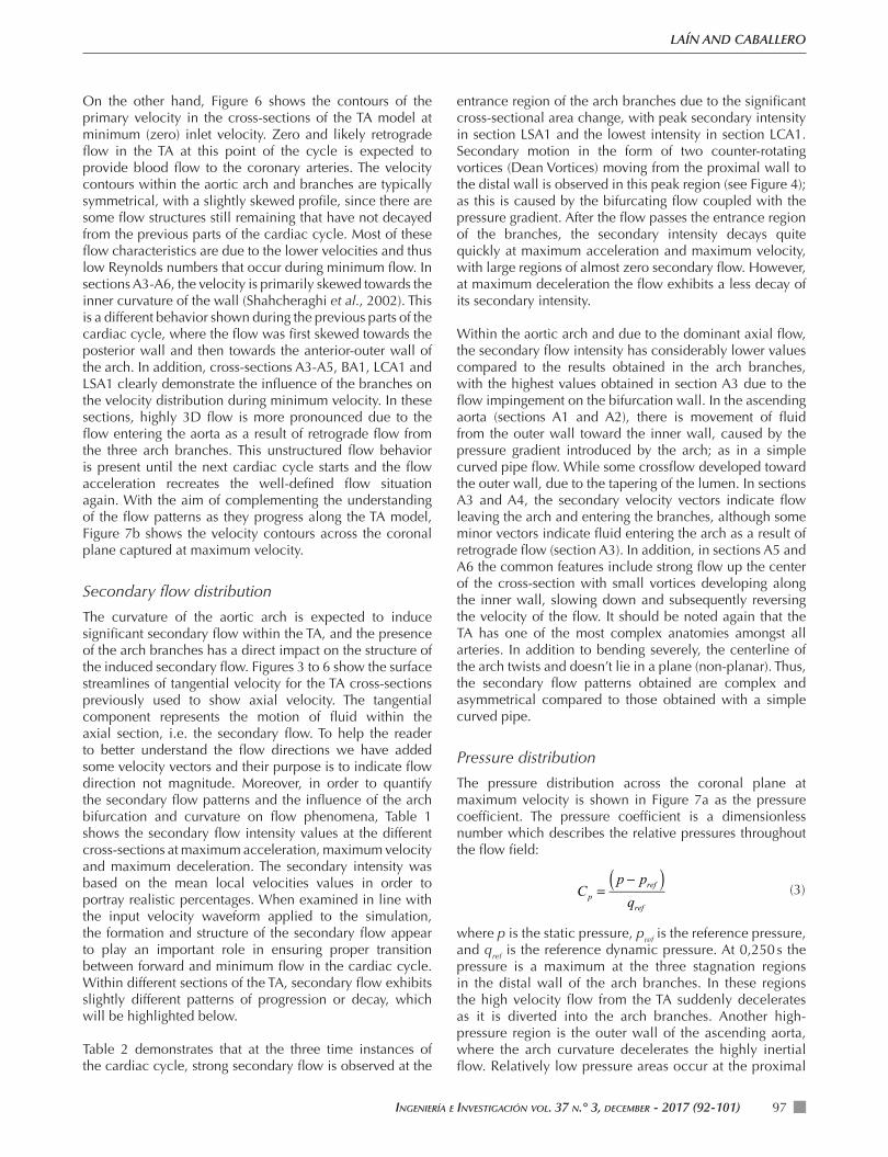
Figure 6. Velocity contours at different cross-sections at minimum velocity. Source: Authors

IngenIería e InvestIgacIón vol. 37 n.° 3, december - 2017 (92-101) 97

LAÍN AND CABALLERO

On the other hand, Figure 6 shows the contours of the primary velocity in the cross-sections of the TA model at minimum (zero) inlet velocity. Zero and likely retrograde flow in the TA at this point of the cycle is expected to provide blood flow to the coronary arteries. The velocity contours within the aortic arch and branches are typically symmetrical, with a slightly skewed profile, since there are some flow structures still remaining that have not decayed from the previous parts of the cardiac cycle. Most of these flow characteristics are due to the lower velocities and thus low Reynolds numbers that occur during minimum flow. In sections A3-A6, the velocity is primarily skewed towards the inner curvature of the wall (Shahcheraghi et al., 2002). This is a different behavior shown during the previous parts of the cardiac cycle, where the flow was first skewed towards the posterior wall and then towards the anterior-outer wall of the arch. In addition, cross-sections A3-A5, BA1, LCA1 and LSA1 clearly demonstrate the influence of the branches on the velocity distribution during minimum velocity. In these sections, highly 3D flow is more pronounced due to the flow entering the aorta as a result of retrograde flow from the three arch branches. This unstructured flow behavior is present until the next cardiac cycle starts and the flow acceleration recreates the well-defined flow situation again. With the aim of complementing the understanding of the flow patterns as they progress along the TA model, Figure 7b shows the velocity contours across the coronal plane captured at maximum velocity.

Secondary flow distribution

The curvature of the aortic arch is expected to induce significant secondary flow within the TA, and the presence of the arch branches has a direct impact on the structure of the induced secondary flow. Figures 3 to 6 show the surface streamlines of tangential velocity for the TA cross-sections previously used to show axial velocity. The tangential component represents the motion of fluid within the axial section, i.e. the secondary flow. To help the reader to better understand the flow directions we have added some velocity vectors and their purpose is to indicate flow direction not magnitude. Moreover, in order to quantify the secondary flow patterns and the influence of the arch bifurcation and curvature on flow phenomena, Table 1 shows the secondary flow intensity values at the different cross-sections at maximum acceleration, maximum velocity and maximum deceleration. The secondary intensity was based on the mean local velocities values in order to portray realistic percentages. When examined in line with the input velocity waveform applied to the simulation, the formation and structure of the secondary flow appear to play an important role in ensuring proper transition between forward and minimum flow in the cardiac cycle. Within different sections of the TA, secondary flow exhibits slightly different patterns of progression or decay, which will be highlighted below.

Table 2 demonstrates that at the three time instances of the cardiac cycle, strong secondary flow is observed at the

entrance region of the arch branches due to the significant cross-sectional area change, with peak secondary intensity in section LSA1 and the lowest intensity in section LCA1. Secondary motion in the form of two counter-rotating vortices (Dean Vortices) moving from the proximal wall to the distal wall is observed in this peak region (see Figure 4); as this is caused by the bifurcating flow coupled with the pressure gradient. After the flow passes the entrance region of the branches, the secondary intensity decays quite quickly at maximum acceleration and maximum velocity, with large regions of almost zero secondary flow. However, at maximum deceleration the flow exhibits a less decay of its secondary intensity.

Within the aortic arch and due to the dominant axial flow, the secondary flow intensity has considerably lower values compared to the results obtained in the arch branches, with the highest values obtained in section A3 due to the flow impingement on the bifurcation wall. In the ascending aorta (sections A1 and A2), there is movement of fluid from the outer wall toward the inner wall, caused by the pressure gradient introduced by the arch; as in a simple curved pipe flow. While some crossflow developed toward the outer wall, due to the tapering of the lumen. In sections A3 and A4, the secondary velocity vectors indicate flow leaving the arch and entering the branches, although some minor vectors indicate fluid entering the arch as a result of retrograde flow (section A3). In addition, in sections A5 and A6 the common features include strong flow up the center of the cross-section with small vortices developing along the inner wall, slowing down and subsequently reversing the velocity of the flow. It should be noted again that the TA has one of the most complex anatomies amongst all arteries. In addition to bending severely, the centerline of the arch twists and doesn’t lie in a plane (non-planar). Thus, the secondary flow patterns obtained are complex and asymmetrical compared to those obtained with a simple curved pipe.

Pressure distribution

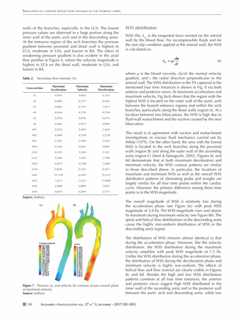
The pressure distribution across the coronal plane at maximum velocity is shown in Figure 7a as the pressure coefficient. The pressure coefficient is a dimensionless number which describes the relative pressures throughout the flow field:

Cp =p − pref( )qref

(3)

where p is the static pressure, pref is the reference pressure, and qref is the reference dynamic pressure. At 0,250 s the pressure is a maximum at the three stagnation regions in the distal wall of the arch branches. In these regions the high velocity flow from the TA suddenly decelerates as it is diverted into the arch branches. Another high-pressure region is the outer wall of the ascending aorta, where the arch curvature decelerates the highly inertial flow. Relatively low pressure areas occur at the proximal

SIMULATION OF UNSTEADY BLOOD FLOW DYNAMICS IN THE THORACIC AORTA

INGENIERÍA E INVESTIGACIÓN VOL. 37 N.° 3, DECEMBER - 2017 (92-101)98

walls of the branches, especially in the LCA. The lowest pressure values are observed in a large portion along the inner wall of the aortic arch and in the descending aorta. At the entrance region of the arch branches the pressure gradient between proximal and distal wall is highest in LCA, moderate in LSA, and lowest in BA. The effect of weakening pressure gradient is also evident in the axial fl ow profi les in Figure 4, where the velocity magnitude is highest in LCA on the distal wall, moderate in LSA, and lowest in BA.

Table 2. Secondary fl ow intensity (%)

Cross-sectionMaximum

AccelerationMaximum Velocity

Maximum Deceleration

A1 0,0793 0,0542 0,1257

A2 0,4899 0,3317 0,2403

A3 0,6043 0,7345 1,4677

A4 0,4364 0,3750 0,5784

A5 0,4158 0,4105 0,6733

A6 0,2666 0,4073 0,8081

BA1 4,2555 4,2893 2,5669

BA2 0,4409 0,1238 2,2258

BA3 0,1401 0,1895 1,2853

BA4 0,1202 0,0322 0,0867

LCA1 0,3553 1,2094 5,1411

LCA2 0,1683 1,1045 1,7998

LCA3 0,0672 0,3388 1,6086

LCA4 0,0294 0,1357 0,5237

LSA1 35,7118 32,4837 25,2711

LSA2 1,6712 1,4123 11,0688

LSA3 0,4080 0,8809 5,6951

LSA4 0,0354 0,2091 2,7571

Source: Authors

Figure 7. Pressure (a), and velocity (b) contours across coronal plane at maximum velocity. Source: Authors

WSS distribution

WSS (Pa), τw, is the tangential force exerted on the arterial wall by the blood fl ow. For incompressible fl uids and for the non-slip condition applied at the arterial wall, the WSS is calculated as:

τW = µ dudr

(4)

where μ is the blood viscosity, du/dr the normal velocity gradient, and r the radial direction perpendicular to the arterial wall. The WSS distribution in the TA captured at the mentioned four time instances is shown in Fig. 8 via both anterior and posterior views. At maximum acceleration and maximum velocity, Fig 8a-b shows that the region with the highest WSS is located on the outer wall of the aortic arch between the branch entrance regions and within the arch branches, particularly along the distal walls (region A). At a location between two bifurcations, the WSS is high due to fl uid-wall reattachment and the suction created by the next bifurcation.

This result is in agreement with suction and reattachment investigations in viscous fl uid mechanics carried out by White (1979). On the other hand, the area with the lowest WSS is located in the arch branches along the proximal walls (region B) and along the outer wall of the ascending aorta (region C) (Mori & Yamaguchi, 2002). Figures 8c and 8d demonstrate that at both maximum deceleration and minimum velocity, the WSS contour patterns are similar to those described above. In particular, the locations of maximum and minimum WSS as well as the overall WSS distribution patterns of alternating peaks and troughs are largely similar for all four time points within the cardiac cycle. However, the primary difference among these time points is in the WSS magnitude.

The overall magnitude of WSS is relatively low during the acceleration phase (see Figure 8a) with peak WSS magnitude of 3,8 Pa. The WSS magnitude rises and attains its maximum during maximum velocity (see Figure 8b). The spiral and helical fl ow distributions in the descending aorta cause the highly non-uniform distribution of WSS in the descending aorta region.

The distribution of WSS remains almost identical to that during the acceleration phase. However, like the velocity distribution, the WSS distribution during the maximum velocity amplifi es with peak WSS magnitude of 7,5 Pa. Unlike the WSS distribution during the acceleration phase, the distribution of WSS during the deceleration phase and minimum velocity is highly non-uniform. The effects of helical fl ow and fl ow reversal are clearly visible in Figures 8c and 8d. Besides the high and low WSS distribution patterns common at all four time instances, the anterior and posterior views suggest high WSS distributed in the inner wall of the ascending aorta and in the posterior wall between the aortic arch and descending aorta, while low

INGENIERÍA E INVESTIGACIÓN VOL. 37 N.° 3, DECEMBER - 2017 (92-101) 99

LAÍN AND CABALLERO

WSS is distributed on the anterior wall of the arch (Wen et al., 2010). Highly non-uniform distribution of WSS is observed in the aortic arch and branching regions. However, the scale of the WSS is lower compared to the WSS during the accelerating phase and maximum velocity, with peak WSS magnitude of 7 Pa during the deceleration phase and peak WSS magnitude of 1,6 Pa during minimum velocity. In conclusion, the regions of maximum and minimum WSS migrate locally with variation in pressure indicating fl uctuation of local WSS with time. The sites with low and fl uctuating WSS are vulnerable for the development of CVDs, such as atherosclerosis.

Conclusions

The main goal of this work was to analyzed and evaluated physiologically relevant hemodynamic parameters of the time dependent fl uid fl ow in a realistic human TA model.

Figure 8. Contours of WSS distribution at (a) maximum acceleration, (b) maximum velocity, (c) maximum deceleration, and (d) minimum velocity. Source: Authors

The obtained fl ow patterns are in agreement with those previously reported in a number of experimental and numerical studies, e.g. (Lantz et al., 2012; Liepsch et al., 1992; Morris et al., 2005; Shahcheraghi et al., 2002; Vasava et al., 2012; Wen et al., 2010). This study offers a detailed graphical presentation and analysis of hemodynamic parameters such as fl ow velocity, stresses and pressures, and this detail can be used in future studies to understand the origin and development of different CVDs. A special care has been taken to improve the visual presentation of the time-dependent results, of particular importance the identifi cation of the primary fl ow fi eld contours, secondary fl ow structures and WSS distribution.

WSS was found to be the lowest along the proximal walls of the arch branches. Earlier studies have established that atherosclerosis is prone to develop in sites in the arteries with low and fl uctuating WSS. This study has revealed that the behavior of the blood fl ow and the distribution of the

Simulation of unSteady blood flow dynamicS in the thoracic aorta

IngenIería e InvestIgacIón vol. 37 n.° 3, december - 2017 (92-101)100

shear forces heavily depend on the complex cardiovascular models, thus there is a pressing need to investigate the impact of patient-specific input data, including various inlet and outlet boundary conditions, such as higher inlet flow velocities or in vivo measured velocities, on the hemodynamic metrics. The numerical simulations in this paper have been made in one of the most complex anatomies of the cardiovascular system, with branching, tapering of lumen and curvature in aortic arch. However, the arterial wall has been assumed to be rigid and approximations have been made for the boundary conditions, although it is known the arterial wall deforms under loads, and in particular for some arteries this deformation is large and should not be approximated by a rigid wall. Since the boundary conditions involve interactions with the upstream and downstream vasculatures absent in the computational domain of interest, physiologically accurate boundary conditions that are robust as well as simple to implement must be carefully considered for each particular problem.

Acknowledgements

A.D. Caballero was supported by the COLCIENCIAS Young Researcher Fellowship. This support is gratefully acknowledged.

References

Caballero, AD., Laín, S. (2013). A Review on Computational Fluid Dynamics Modelling in Human Thoracic Aorta. Cardiovascular Engineering and Technology, 4, 103-130.

Caballero, AD., Laín, S. (2015). Numerical Simulation of non-Newtonian Blood Flow Dynamics in Human Thoracic Aorta. Computer Methods in Biomechanics and Biomedical Engineering, 18, 1200-1216.

Cecchi, E., Giglioli, C., Valente, S., Lazzeri, C., Gensini, G.F., Abbate, R., Mannini, L. (2011). Role of hemodynamic shear stress in cardiovascular disease. Atherosclerosis., 214, 249-256.

Chandran, K.B. (1993). Flow Dynamics in the Human Aorta. J Biomech Eng., 115, 611–616.

Dabagh, M., Vasava, P., & Jalali, P. (2015). Effects of severity and location of stenosis on the hemodynamics in human aorta and its branches. Medical & biological engineering & computing, 53(5), 463-476.

Fung, Y.C. (1997). Biomechanics Circulation. 2nd ed. Springer.

Gallo, D., Gülan, U., Di Stefano, A., Ponzini, R., Lüthi, B., Holzner, M., & Morbiducci, U. (2014). Analysis of thoracic aorta hemodynamics using 3D particle tracking velocimetry and computational fluid dynamics. Journal of biomechanics, 47(12), 3149-3155.

Kern, M.J., Lim, M.J., Goldstein, J.A. (2009). Hemodynamic Rounds: Interpretation of Cardiac Pathophysiology from Pressure Waveform Analysis Transport Phenomena in the Cardiovascular System. 3rd ed. Wiley-Blackwell.

Kilner, P.J., Yang, G.Z., Mohiaddin, R.H., Firmin, D.N., Longmore, D.B. (1993). Helical and retrograde secondary flow patterns in the aortic arch studied by three-directional magnetic resonance velocity mapping., Circulation. 88(5), 2235-2247.

Liu, X., Fan, Y., Deng, X., Zhan, F. (2011). Effect of non-Newtonian and pulsatile blood flow on mass transport in the human aorta. J Biomech., 44(6), 123-1131.

Liepsch, D., Moravec, S.T., Baumgart, R. (1992). Some flow visualization and laser-Doppler velocity measurements in a tube-to-scale elastic model of a human arotic arch—a new model technique. Biorheology., 29, 563–580.

Lantz, J., Gardhagen, R., Karlsson, M. (2012). Quantifying turbulent wall shear stress in a subject specific human aorta using large eddy simulation. Med Eng Phys., 34, 1139-1148.

Middleman, S. (1972). Transport Phenomena in the Cardiovascular System. 1st ed. John Wiley and Sons.

Morbiducci, U., Ponzini, R., Rizzo, G., Cadioli, M., Esposito, A., Montevecchi, F.M., Redaelli, A. (2011). Mechanistic insight into the physiological relevance of helical blood flow in the human aorta. An in vivo study. Biomech Model Mechanobiol, 10, 339–355.

Morbiducci, U., Ponzini, R., Gallo, D., Bignardi, C., Rizzo, G. (2013). Inflow boundary conditions for image-based computational hemodynamics: impact of idealized versus measured velocity profiles in the human aorta. J Biomech., 46, 102-109.

Morris, L., Delassus, P., Callanan, A., Walsh, M., Wallis, F., Grace, P., McGloughlin, T. (2005). 3-D numerical simulation of blood flow through models of the human aorta. J. Biomech Eng., 127, 767-775.

Mori, D., & Yamaguchi, T. (2002). Computational fluid dynamics modeling and analysis of the effect of 3-D distortion of the human aortic arch. Computer Methods in Biomechanics & Biomedical Engineering, 5(3), 249-260.

Nerem, R.M., Rumberger, J.A., Gross, D.R., Hamlin, R.L., Geiger, G.L. (1974). Hot-Film Anemometry Velocity Measurements of Arterial Blood Flow in Horses. CircRes, 10, 301–313.

Park, Y.J., Park, C.Y., Hwang, C.M., Sun, K., Min, B.G., (2007). Pseudo-organ boundary conditions applied to a computational fluid dynamics model of the human aorta. Comput. Biol., Med. 37, (8), 1063-1072.

Pedley, T.J. (1980). The Fluid Mechanics of Large Blood Vessels. Cambridge University Press, Cambridge.

Prakash, S., Ethier, C.R. (2001). Requirements for mesh resolution in 3D computational hemodynamics. J. Biomech Eng., 23, 134–144.

Seed, W.A., Wood, N.B. (1971). Velocity Patterns in the Aorta. Cardiovasc, Res. 5, 319–330.

Shahcheraghi, N., Dwyer, H.A., Cheer, A.Y., Barakat, AI., Rutanganira, T. (2002). Unsteady and three-dimensional simulation of blood flow in the human aortic arch. J. Biomech Eng., 124, 378-87.

Simbios project, (2007). Retrieved from: https://simtk.org/xml/index.xml, http://simbios.stanford.edu/

IngenIería e InvestIgacIón vol. 37 n.° 3, december - 2017 (92-101) 101

LAÍN AND CABALLERO

Vasava, P., Jalali, P., Dabagh, M., Kolari, P. (2012). Finite element modelling of pulsatile blood flow in idealized model of human aortic arch: Study of hypotension and hypertension. Comp. Math. Methods in Medicine., 2012, Article ID 861837.

Versteeg. H.K., Malalasekera, W. (2007). An introduction to computational fluid dynamics. The finite volume method. Pearson, London.

Wen, C.Y., Yang, A.S., Tseng, L.Y.,Chai, JW. (2010). Investigation of Pulsatile flow field in healthy thoracic aorta models. Ann Biomed Eng., 38, 391-402.

White, F. M. (1979). Viscous Fluid Flow, McGraw-Hill, New York.

Womersley, J.R. (1955). Method for the calculation of velocity, rate of flow and viscous drag in arteries when the pressure is known. J Physiol., 127, 553–563.