simulation of tropical pacific and atlantic oceans … · simulation of tropical pacific and...
TRANSCRIPT
www.elsevier.com/locate/ocemod
Ocean Modelling 9 (2005) 253–282
Simulation of tropical Pacific and Atlantic Oceans using aHYbrid Coordinate Ocean Model
C. Shaji a, C. Wang b,*, G.R. Halliwell Jr. c, A. Wallcraft d
a Cooperative Institute for Marine and Atmospheric Studies, University of Miami, Miami, FL, USAb Physical Oceanography Division, NOAA Atlantic Oceanographic and Meteorological Laboratory, 4301
Rickenbacker Causeway, Miami, FL 33149, USAc Rosenstiel School of Marine and Atmospheric Science, University of Miami, Miami, FL, USA
d Naval Research Laboratory, Stennis Space Center, Mississippi, USA
Received 22 November 2003; received in revised form 24 May 2004; accepted 14 July 2004
Available online 13 September 2004
Abstract
The climatological annual cycle of the tropical Pacific and Atlantic Oceans is simulated using the HYbrid
Coordinate Ocean Model (HYCOM) configured in a non-uniform horizontal grid spanning 30�S–65.5�Nand 102�E–15�E. The model is initialized with climatological summer temperature and salinity and is forced
by climatological atmospheric fields derived from the COADS and ECMWF ERA-15 reanalysis. Themodel is spun up for 20 years to reach a reasonable steady state in the primary region of interest from
20�S to 20�N, and year 20 is analyzed. The COADS simulation is primarily analyzed because it is slightly
better in more respects than the ECMWF simulation, particularly in the representation of upper-ocean
thermal structure. The model generally reproduces the seasonal variability of major circulation features
in both oceans reasonably well when compared to climatologies derived from several observational datasets
(surface drifters, TAO mooring array, COADS, Levitus, Pathfinder SST), and when compared to other
model simulations. Model evaluation is complicated by the fact that the different climatologies, including
the atmospheric reanalysis climatologies that drive the model, are averaged over different time intervals. Inthe tropics, the model thermocline reproduces the observed zonal slopes and meridional ridges/troughs in
the thermocline. The simulated Equatorial Undercurrent compares favorably to observations, but is
slightly deeper than observed. The model overestimates temperature in the Pacific warm pool regions, both
1463-5003/$ - see front matter � 2004 Elsevier Ltd. All rights reserved.
doi:10.1016/j.ocemod.2004.07.003
* Corresponding author. Tel.: +1 305 361 4325; fax: +1 305 361 4412.
E-mail address: [email protected] (C. Wang).

254 C. Shaji et al. / Ocean Modelling 9 (2005) 253–282
west and east, by more than 1�C when compared to all observed climatologies. The model also tends to
overestimate temperature in the eastern equatorial cold tongues in both the Atlantic and Pacific, with this
overestimate being confined to a very small region of the far eastern Pacific during winter. This overesti-
mate varies substantially depending on which observed climatology is used for the comparison, so model
limitations are only partly responsible for the simulated–observed temperature differences in the cold
tongues.
� 2004 Elsevier Ltd. All rights reserved.
Keywords: HYCOM; Non-uniform grid; Tropical circulation; Simulation; Observed data
1. Introduction
Many studies have been performed using ocean models of various types to study the tropicalPacific and Atlantic Ocean circulation. Busalacchi and O�Brien (1980) used a linear, reducedgravity model without thermodynamics to simulate the equatorial current system in the tropicalPacific. The study revealed that linear dynamics is sufficient to understand many aspects of theinfluence of equatorially trapped Rosssby and Kelvin waves on the equatorial current system.Their relatively simple model was therefore capable of reproducing the location and variabilityof equatorial surface currents, but not important thermodynamical processes. Philander et al.(1987) forced a level coordinate primitive equation ocean general circulation model (OGCM)with seasonally varying climatological fields to study the mass and heat budget of the tropicalPacific. Broad features of the seasonal variability of the equatorial surface circulation and thethermocline movements were realistically obtained from their model study. Philander and Paca-nowski (1986) used this same model to study the upper-ocean seasonal cycle of the tropicalAtlantic.
Vertical mixing is very important for accurately simulating the baroclinic structure and flowfield of the tropical ocean using OGCMs. Chen et al. (1994) studied the tropical circulation inthe Pacific Ocean by embedding three different vertical mixing schemes in a 3-D ocean model.The mixing algorithms considered in their study are the Mellor–Yamada (MY) level 2.5 turbu-lence closure model (Mellor and Yamada, 1982), the Kraus–Turner (KT) bulk model (Turnerand Kraus, 1967; Niiler and Kraus, 1977), and a hybrid method where Richardson numberinstability mixing from the dynamical instability model of Price et al. (1986) was included withthe KT model to provide mixing beneath the bulk mixed layer. The hybrid scheme generatedmore realistic circulation features in the equatorial Pacific Ocean than the other mixing models.Murtugudde et al. (1995) applied a reduced gravity, isopycnal vertical coordinate ocean modelto the three tropical oceans, neglecting salinity effects on density and representing the surfacemixed layer by a constant depth layer. Individual simulations forced with climatic winds andsurface heat fluxes based on observed sea surface temperature (SST) were conducted separatelyin the tropical Atlantic, Pacific, and Indian Oceans. The model reproduced most of the wind-driven currents and many features of the thermocline such as the annual cycle of zonal andmeridional thermocline slope. However, the surface heat flux and vertical mixing parameteriza-tions used in their model produced unrealistic SSTs, especially in the western boundary currentregions.
C. Shaji et al. / Ocean Modelling 9 (2005) 253–282 255
It is important to further improve OGCMs to accurately simulate important climate processesoccurring in the tropical ocean such as shallow meridional overturning cells. These cells areresponsible for supplying water to the Equatorial Undercurrent (EUC) in both the Atlanticand Pacific Oceans. For example, Lu et al. (1998) investigated Pacific shallow overturning cellsin a layer model study, documenting the importance of tropical and subtropical overturning cellsin both the North and South Pacific for contributing water to the EUC. The present study revisitsthese and other issues by simulating the climatological annual cycles of the tropical Atlantic andPacific Oceans using a new ocean general circulation model, specifically the HYbrid CoordinateOcean Model (HYCOM; Bleck, 2002; Chassignet et al., 2003; Halliwell, 2004). This model con-tains a hybrid level-isopycnic-sigma vertical coordinate and contains several state-of-the-art ver-tical-mixing submodels. HYCOM has evolved from the Miami Isopycnic Coordinate OceanModel (MICOM). Chassignet et al. (1996) compared MICOM to the GFDL level-coordinatemodel (Cox, 1984) in the Atlantic Ocean to demonstrate the advantages of isopycnic vertical coor-dinates in long climate integrations, particularly in regards to the inability of level coordinatemodels to retain their most dense water masses and produce a realistic meridional overturning cir-culation. Also, the MICOM simulation generated a stronger EUC that compared more favorablyto observations than the GFDL model. HYCOM was created to correct known shortcomings ofMICOM vertical coordinate system, which consists of isopycnic layers capped by a single slabmixed layer. In particular, isopycnic coordinates provide little or no vertical resolution in regionswith weak stratification, including the surface mixed layer. HYCOM is designed to retain theadvantages of isopycnic coordinates as much as possible in the open stratified ocean, but to trans-form into level (pressure) coordinates in unstratified regions such as the surface mixed layer, andalso transform to terrain-following (sigma) coordinates in the coastal ocean.
Further details of the HYCOM equations and numerical algorithms, along with a descriptionand validation of the hybrid coordinate generator, can be found in Bleck (2002). The several ver-tical mixing choices embedded in HYCOM are described and initially evaluated by Halliwell(2004). He demonstrates that the K-Profile Parameterization (KPP; Large et al., 1994), NASAGISS level 2 turbulence closure, MY level 2.5 turbulence closure, and Price et al. (1986) dynamicalinstability model all perform reasonably well in low resolution climatic simulations. Chassignetet al. (2003) demonstrate the flexibility of the hybrid grid generator by comparing HYCOMrun in its default hybrid mode to HYCOM run as a level-coordinate and isopycnic-coordinatemodel. They also demonstrate the advantages of referencing HYCOM potential density tomid-depth pressure (20MPa) and using the thermobaric compressibility correction of Sun et al.(1999) to calculate the pressure gradient force.
MICOM/HYCOM studies to date have focused primarily on middle and high latitude proc-esses. In this study, we use HYCOM configured on a non-uniform grid to document the annualcycle of upper-ocean stratification and circulation in the tropical Pacific and Atlantic Oceans. Themain goal is to evaluate HYCOM tropical ocean simulations when configured on a non-uniformgrid designed to provide maximum meridional resolution near the equator. Since model errorsand biases will be caused in part by errors and biases in the climatological forcing, this sensitivityis also examined by driving it with both the COADS climatology (Woodruff et al., 1987) and theECMWF ERA-15 reanalysis climatology (Gibson et al., 1999). This initial study is designed toprovide baseline results for planned HYCOM studies designed to evaluate sensitivity to verti-cal mixing choice, vertical coordinate distribution, and other HYCOM subgrid-scale

256 C. Shaji et al. / Ocean Modelling 9 (2005) 253–282
parameterizations. For example, HYCOM has recently been equipped with three new horizontaladvection algorithms in addition to the MPDATA (Multidimensional Positive Definite AdvectionTransport Algorithm) used previously in MICOM and HYCOM. In Section 2, we describe themodel configuration, the experiments, and the observations used to validate model results. Thesimulated tropical ocean circulation in the Pacific and Atlantic basins using COADS (Woodruffet al., 1987) forcing are evaluated in Sections 3 and 4 respectively. In Section 5, the COADSand ECMWF ERA-15 reanalysis simulations are compared to demonstrate that the COADS re-sults are generally more realistic. Conclusions are presented in Section 6.
2. Model and observations
The HYCOM configuration for the numerical experiments, along with the observations usedfor comparison and validation, are described first.
2.1. Model configuration and numerical experiments
The computational domain spans the Pacific and Atlantic basins from 30�S to 65.5�N and102�E to 15�E. The standard Mercator grid configuration used in earlier MICOM/HYCOM stud-ies has been modified. The zonal grid resolution remains a uniform 0.72�, but the meridional gridresolution is set to 0.36� between 5�S and 5�N to improve the resolution of zonal equatorial cur-rents. Poleward of 10�S and 10�N, the standard square Mercator grid is used where meridionalresolution is 0.72cosu, where u is latitude. Meridional resolution therefore gradually decreasesfrom 0.36� to 0.72� in the bands from 5�S to 10�S and from 5�N to 10�N. The model is configuredwith 22 layers. Since we are interested exclusively in upper-ocean processes, we use a surface ref-erence pressure for our target potential density (rh) values of 19.50, 20.25, 21.00, 21.75, 22.50,23.25, 24.0, 24.70, 25.28, 25.77, 26.18, 26.52, 26.80, 27.03, 27.22, 27.38, 27.52, 27.64, 27.74,27.82, 27.88, and 27.94. The target densities of the top five layers are chosen to be lighter thanwater encountered almost everywhere in the ocean so that they exist as level coordinates at thesurface and provide reasonable vertical resolution in the surface mixed layer. The bottom topog-raphy is based on ETOPO5 data. The KPP vertical mixing model (Large et al., 1994) is used. De-tails regarding the implementation of KPP in HYCOM can be found in Halliwell (2004).
The model is initialized with summer temperature and salinity from the Levitus monthly clima-tology (Levitus and Boyer, 1994; Levitus et al., 1994) and run for 20 years. It is driven by monthlywind stress, wind speed, surface air temperature, surface atmospheric specific humidity, net short-wave radiation, net longwave radiation and precipitation fields obtained from both the COADSclimatological dataset and ECMWF ERA-15 atmospheric reanalysis climatology. The sensibleand latent heat fluxes are calculated during model runs using the model sea surface temperature(SST) and the same bulk aerodynamic formulae used in MICOM (Langlois et al., 1997). Thenorthern and southern edges of the model domain are treated as closed boundaries. Boundaryconditions are provided by buffer zones that are ten grid points wide within which temperature,salinity, and interface depth are relaxed to Levitus climatological values that have been verticallyremapped to hybrid vertical coordinates. The relaxation time scale increases from 20 to 120 dayswith distance away from the boundaries.
C. Shaji et al. / Ocean Modelling 9 (2005) 253–282 257
Fields from the final year of the simulations (year 20) are analyzed here. For the purpose ofconducting model–data comparisons, the simulated fields stored on the hybrid vertical coordi-nates are re-mapped onto level coordinates using vertical linear interpolation. In the following dis-cussions in this article, wherever we mention seasons (winter, spring, summer and fall), we meanthe boreal ones unless and otherwise specified.
2.2. Observations
We use several observational data sets to evaluate the model simulations. First, satellite-trackedsurface drifters drogued at a depth of 15m (Niiler, 2001) are compared to the simulated upper-ocean currents and temperature at 15m. Climatological mean fields of surface currents andtemperature are calculated from the drifters. The drifter observations of surface current aredecomposed into a time-mean field, seasonal harmonics (annual and semi-annual) and a residualeddy field characterized by a finite integral time scale (Lumpkin, 2003). Climatological values for agiven day are constructed from the time-mean field and the seasonal harmonics. From these, themonthly mean maps of currents and temperature are constructed. Further details regarding thiscalculation can be found in Lumpkin (2003).
In the Pacific Ocean, Acoustic Doppler Current Profiler (ADCP) horizontal velocity data areavailable from the Tropical Atmosphere Ocean (TAO) array (McPhaden et al., 1998). To evaluatethe simulations, we use zonal velocity data from four of these arrays located in the easternequatorial Pacific (110�W, 0�), east-central equatorial Pacific (140�W, 0�), west-central equatorialPacific (170�W, 0�) and western equatorial Pacific (165�E, 0�). At these points monthly climato-logical velocities are prepared using daily data from 1991 to 2000. ADCP current data are pres-ently unavailable in the equatorial Atlantic Ocean.
Also in the Pacific Ocean, daily subsurface temperature data are available along the equatorfrom TAO moorings at 147�E, 156�E, 165�E, 180�W, 170�W, 155�W, 140�W, 125�W, 110�Wand 95�W.We prepared the climatological monthly mean temperature at each location using dailydata from 1991 to 2000 that were interpolated to fixed standard depths of 1, 10, 25, 50, 75, 100,125, 150, 175, 200, 250, 300 and 500m, and then gridded to 1� resolution from 147�E to 95�W. Inthe tropical Atlantic, we compare the Levitus (Levitus and Boyer, 1994) subsurface temperaturedata to the simulated temperature.
Sea surface temperature (SST) from the model is compared to SST from the Pathfinder (Caseyand Cornillon, 1999) dataset. The NASA-funded SST Pathfinder project (Evans and Podesta,1996) is designed to generate an accurate and consistent global SST dataset from measurementsmade by the AVHRR infrared instrument flown on NOAA satellites since November 1981. In situSST measurements are used to optimize coefficients in the equation used to calculate PathfinderSST from irradiance measurements in multiple infrared channels. SST fields are produced by firstcomputing 4-km resolution Global Area Coverage (GAC) AVHRR SST retrievals, then binningcloud free retrievals into 9km equal area fields twice daily (day and night). The global fields showzero bias and 0.5 �C rms with respect to cotemporal 1m temperature measured by buoys. The cli-matology was created by averaging into monthly means, then calculating climatological monthlymeans over the 1985–1997 time interval. Both daytime and nighttime daily fields are included ineach monthly average. A 7 · 7 point median filter is applied to fill in many of the gaps, and a 7 · 7point median smoother is used for the entire field to remove small-scale noise.
258 C. Shaji et al. / Ocean Modelling 9 (2005) 253–282
3. Circulation in the tropical Pacific Ocean
The simulated circulation in the tropical Pacific Ocean is compared to observations, focusingfirst on the surface flow pattern and then on the subsurface structure.
3.1. Surface circulation
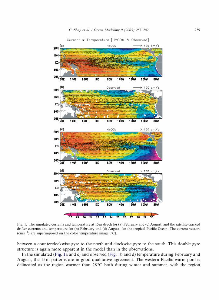
The surface circulation in the tropical Pacific Ocean is driven primarily by the trade wind pat-tern and consists of alternating bands of eastward and westward flowing zonal currents. Theseinclude the westward South Equatorial Current (SEC) and North Equatorial Current (NEC),which are the largest and most persistent zonal currents. The eastward flowing North EquatorialCountercurrent (NECC) and South Equatorial Countercurrent (SECC) often interrupt thesebroad westward flows. The strength and latitude bands of these currents depend strongly onthe seasonal variability in the wind stress forcing. Fig. 1a and c display the simulated currentsand temperature at 15m during February and August while Fig. 1b and d display the correspond-ing fields derived from satellite-tracked drifters. From Fig. 1a and b similar major current featuresare present in both the model and observations during February. Simulated surface currents tendto be stronger than observed near the equator, but weaker away from the equator where merid-ional resolution is lower. The simulated SEC generally extends northward to about 5�N except inthe far western Pacific where southeastward boundary flow exists south of the equator in both thesimulation and observations and extends eastward into the interior from 8 to 12�S to about themiddle of the basin as the SECC. In the eastern Pacific south of 10�S the model SEC is weakerthan observed. Near the equator, both the model and observed SEC accelerates from the easternPacific to around 170�W with the surface divergence associated with equatorial upwelling clearlyevident. The maximum SEC velocity reaches about 60cms�1 in the model and 70cms�1 in theobservations although simulated currents tend to be stronger than observed over most of the trop-ical Pacific within a few degrees of the equator. The westward flowing NEC is evident north of10�N in both the simulation and observations, and tends to weaken northward towards 20�N. Be-tween 5�N and 10�N, the narrow eastward NECC extends across nearly the full width of theocean. The simulated NEC and NECC are both weaker than observed.
The equatorial current system shows more seasonal variation in the western half of the basin.The simulated and observed NEC is weaker in August than in February because the NorthernHemisphere trade winds are weaker then. The simulated and observed SEC spans the full widthof the ocean south of 5�S during August (Fig. 1c and d), with no SECC evident. In the westernPacific, the simulated and observed flow is eastward between 3�N and equator. The SEC in thecentral and eastern part of the basin is more intense during August because the southeasterlytrades are stronger in boreal summer. The simulated and observed SEC attains a maximum veloc-ity of about 1ms�1 along the equator in August, but simulated flow tends to be stronger than ob-served near the equator west of about 130�W. As during February, the August SEC accelerates inthe eastern Pacific to about 160�W with equatorial divergence clearly evident. The SEC turnsnorth of the equator around 150�W, and then eastward to supply water to the NECC and thusclose the western end of an anticyclonic (equatorial) gyre. This northward turn is clearer in thesimulation than in the observations. The NECC water eventually turns southward and westwardat the eastern end of the basin to close this equatorial gyre. West of about 180�, the NECC flows
(d)
(c)
(b)
(a)
Fig. 1. The simulated currents and temperature at 15m depth for (a) February and (c) August, and the satellite-tracked
drifter currents and temperature for (b) February and (d) August, for the tropical Pacific Ocean. The current vectors
(cms�1) are superimposed on the color temperature image (�C).
C. Shaji et al. / Ocean Modelling 9 (2005) 253–282 259
between a counterclockwise gyre to the north and clockwise gyre to the south. This double gyrestructure is again more apparent in the model than in the observations.
In the simulated (Fig. 1a and c) and observed (Fig. 1b and d) temperature during February andAugust, the 15m patterns are in good qualitative agreement. The western Pacific warm pool isdelineated as the region warmer than 28�C both during winter and summer, with the region
260 C. Shaji et al. / Ocean Modelling 9 (2005) 253–282
expanding northward to cover a much larger area during summer. This warm pool tends to bewarmer in the simulations. In the eastern Pacific, warm water is also encountered off the coastof Central America during summer, a region considered to be part of the Western Hemispherewarm pool (Wang and Enfield, 2001, 2003). This warm pool also tends to be warmer in the simu-lations. In February, the model produces a cold equatorial tongue in the eastern Pacific that iscolder than observed. During summer, the eastern equatorial Pacific displays an intense coldwater tongue with temperature around 22�C in both the simulation and observations, extendingfarther to the west in the simulation, that is mainly a result of eastern equatorial upwelling com-bined with westward advection of the cold water by the SEC. The southeastern region is also cov-ered by cold water, which intensifies during boreal summer when the temperature drops to almost18�C. This cold water is partly a result of the upwelling occurring along the coast of Peru plusoffshore advection by the SEC.
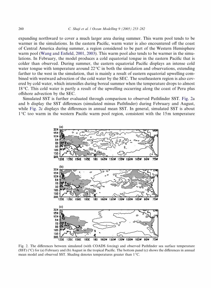
Simulated SST is further evaluated through comparison to observed Pathfinder SST. Fig. 2aand b display the SST differences (simulated minus Pathfinder) during February and August,while Fig. 2c displays the differences in annual mean SST. In general, simulated SST is about1�C too warm in the western Pacific warm pool region, consistent with the 15m temperature
(a)
(b)
(c)
Fig. 2. The differences between simulated (with COADS forcing) and observed Pathfinder sea surface temperature
(SST) (�C) for (a) February and (b) August in the tropical Pacific. The bottom panel (c) shows the differences in annual
mean model and observed SST. Shading denotes temperatures greater than 1 �C.

C. Shaji et al. / Ocean Modelling 9 (2005) 253–282 261
comparison in Fig. 1. Simulated SST tends to be too warm in the eastern equatorial cold tongueregion to the east of about 130�W during August, again consistent with the 15m temperaturecomparison in Fig. 1. The February comparison in Fig. 2a indicates that simulated cold tongueSST is too warm only in a small band east of 105�W. This is not consistent with the 15m temper-ature comparison, which indicates that simulated SST is generally too cold to the east of 140�W.This inconsistency could result in part from the different temporal averaging intervals of the twotemperature climatologies. This question is further assessed in Section 5, where Levitus and Path-finder SST are compared. In other regions, SST differences are small.
The observed temperature differences undoubtedly result in part from model biases, but forcingbiases are also likely important. Recently, scientists at NOAA/AOML have processed a new forc-ing climatology from the Southampton Oceanography Centre where constraints have been usedto correct the surface thermal forcing fields. HYCOM simulations forced with this new climatol-ogy reproduced thermal variability in the Atlantic warm pool with improved accuracy. Forcingbias also results from the use of monthly fields to drive the model and not high-frequency fieldsthat resolve synoptic and diurnal variability.
Fig. 3 (a, b) and (c, d) show seasonal variations of surface zonal currents at 165�E and 110�Wobtained from the model and drifter data respectively. Although broad agreement is evident inobserved and simulated patterns, differences do exist in the location and strength of currents.At 165�E, simulated and observed westward flow associated with the NEC exists north of about9�N, but eastward flow appears in the simulation north of about 18�N. This reversal occurs northof 20�N in the observations except during summer when the reversal occurs just south of 20�N(Fig. 3c). The model qualitatively reproduces observed semi-annual reversals of near-equatorialflow direction. The model generally underestimates current speeds south of about 10�S. An excep-tion to this is the eastward SECC observed between 6�S and 12�S during winter, which the modelreproduces realistically. Tomczak and Godfrey (1994) observed that the SECC is strongest in bor-eal winter with its strength gradually decreasing from west to east so that it is confined primarilyto the western and central Pacific.
At 110�W, the model generally underestimates current speeds at all latitudes. The observedSEC reverses to eastward flow at the equator during spring (Fig. 3d) while the simulated flow be-comes very weak but does not reverse (Fig. 3b). Although the disagreement likely results in partfrom model biases, forcing bias also contributes as illustrated in Section 5, where the COADS andECMWF simulations are compared.
3.2. Subsurface circulation
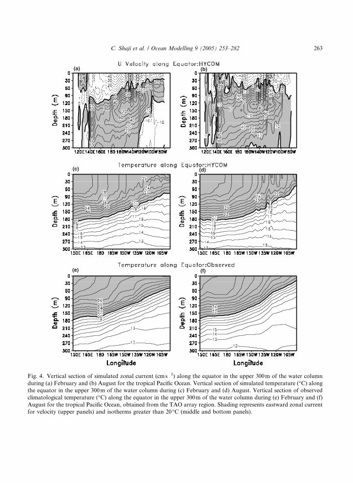
Fig. 4 (a and b) depict vertical sections of model zonal currents in the upper 300m along theequator during February and August. During February, the SEC is generally confined above30m in the eastern Pacific, but gradually thickens toward the west to about 100m west of140�E. Eastward zonal flow exists in the upper 60m at the western end of the domain. In August,the SEC only extends westward to 160�E, and it thickens toward the east. Below the surface, thesimulated EUC core is deep in the western Pacific and slopes upward to the east, with a largerslope during winter, as has been observed in earlier observational and modeling studies. In Feb-ruary the core velocity maximum of about 80cms�1 is located at 140�W at a depth of about120m. In August, two core velocity maxima exist (80cms�1 at 120�W, 120m depth; 100cms�1

(a)
(c) (d)
(b)
Fig. 3. Seasonal variations of the simulated zonal surface current along (a) 165�E and (b) 110�W. Seasonal variations of
the observed satellite-tracked drifter zonal surface current along (c) 165�E and (d) 110�W. The unit of current is cms�1.
Shading denotes eastward zonal current.
262 C. Shaji et al. / Ocean Modelling 9 (2005) 253–282
at 150�W, 120m depth). In other model simulations, Murtugudde et al. (1996) obtained a corevelocity of 160cms�1 during March and Philander et al. (1987) obtained a core velocity of150cms�1 during May. Measured core velocity maxima tend to be smaller than this, but largerthan the values simulated by HYCOM. Yu and McPhaden (1999) reported a core velocity max-imum of 90cms�1. This issue is discussed further in Section 3.3.
Fig. 4 (c, d) and (e, f) show the vertical sections of temperature along the equator during Feb-ruary and August from the simulation and the TAO array observations (Section 2) respectively. Acomparison between Fig. 4 (c, d) and (e, f) indicates that the simulated temperature structureagrees rather well with the observed temperature structure along the equator. In particular, thesimulation generally reproduces the depth and strength of the thermocline, along with its upwardslope to the east, quite realistically. As a result, the model should accurately reproduce the result-ing eastward zonal pressure gradient force along the equator that maintains the EUC (Philander,1990). On the negative side, model isotherms tend to be deeper than observed, particularly be-neath the thermocline. Also, the model underestimates the thickness of the thermocline east ofabout 120�W as isotherms at the base of the thermocline and below become flat instead of con-tinuing the observed upward slope to the east of this longitude.
(a) (b)
(c) (d)
(e) (f)
Fig. 4. Vertical section of simulated zonal current (cms�1) along the equator in the upper 300m of the water column
during (a) February and (b) August for the tropical Pacific Ocean. Vertical section of simulated temperature (�C) alongthe equator in the upper 300m of the water column during (c) February and (d) August. Vertical section of observed
climatological temperature (�C) along the equator in the upper 300m of the water column during (e) February and (f)
August for the tropical Pacific Ocean, obtained from the TAO array region. Shading represents eastward zonal current
for velocity (upper panels) and isotherms greater than 20 �C (middle and bottom panels).
C. Shaji et al. / Ocean Modelling 9 (2005) 253–282 263
(a) (b)
(c) (d)
(e) (f)
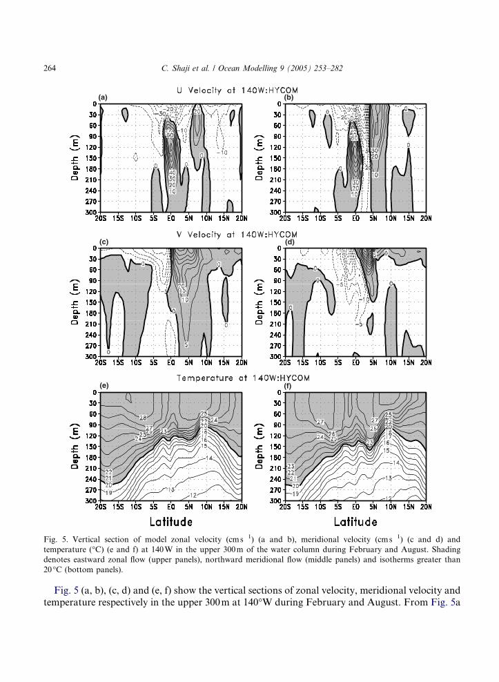
Fig. 5. Vertical section of model zonal velocity (cms�1) (a and b), meridional velocity (cms�1) (c and d) and
temperature (�C) (e and f) at 140W in the upper 300m of the water column during February and August. Shading
denotes eastward zonal flow (upper panels), northward meridional flow (middle panels) and isotherms greater than
20 �C (bottom panels).
264 C. Shaji et al. / Ocean Modelling 9 (2005) 253–282
Fig. 5 (a, b), (c, d) and (e, f) show the vertical sections of zonal velocity, meridional velocity andtemperature respectively in the upper 300m at 140�W during February and August. From Fig. 5a
C. Shaji et al. / Ocean Modelling 9 (2005) 253–282 265
and b, the SEC is confined above 40m at the equator while it penetrates to deeper levels to thenorth and south. The strongest westward flow associated with the SEC is mainly concentrated be-tween about 5�S and 5�N. In the Southern Hemisphere, weaker westward surface zonal flow existssouthward to 20�S. In the Northern Hemisphere, weaker westward zonal flow extends northwardto 20�N during February with the exception of eastward flow associated with the NECC near 8�Nthat has a maximum near 50m and is relatively weak at the surface. During August, a strong east-ward flowing NECC exists between 5 and 10�N with maximum speeds exceeding 40cms�1 above90m. Just below the surface SEC, the eastward flowing subsurface EUC is confined between 2�Sand 2�N with maximum velocity exceeding 80cms�1 at 120m during February and 135m duringAugust. During February, strong equatorial divergence between 2�S and 2�N is primarily con-fined above 100m (Fig. 5c). There is no clear transition between the surface divergence and qua-si-geostrophic convergence beneath it. Near surface meridional convergence is present between 5and 15�S, and also between 6 and 14�N, which could be associated with the downwelling limbs ofshallow overturning cells. During August, the axis of equatorial divergence is tilted, being on theequator at the surface, but shifting northward with depth to 3�N at 120m. Strong meridional con-vergence exists from 2 to 5�S and from 4 to 7�N, suggesting that strong shallow tropical overturn-ing cells may exist during summer.
The vertical structure of temperature at 140�W (Fig. 5e and f) shows the classical pattern in-ferred from earlier studies (Philander, 1990), with a shallower thermocline in the equatorial regionand a trough-ridge system north of the equator associated with the NECC that is stronger duringsummer. South of 3�S and north of 10�N, the poleward increases in isotherm depth reflects thegeostrophic balance associated with the westward-flowing SEC and NEC, respectively. Theupward (downward) bowing of isotherms above (below) the EUC core within 2� of the equatorreflects the equatorial quasi-geostrophic balance associated with the EUC and the SEC jet above(Philander, 1990).
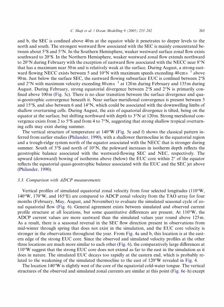
3.3. Comparison with ADCP measurements
Vertical profiles of simulated equatorial zonal velocity from four selected longitudes (110�W,140�W, 170�W, and 165�E) are compared to ADCP zonal velocity from the TAO array for fourmonths (February, May, August, and November) to evaluate the simulated seasonal cycle of zo-nal equatorial flow (Fig. 6). General agreement exists between simulated and observed currentprofile structure at all locations, but some quantitative differences are present. At 110�W, theADCP current values are more eastward than the simulated values year round above 125m.As a result, there is a seasonal reversal in the SEC flow direction present in observations frommid-winter through spring that does not exist in the simulation, and the EUC core velocity isstronger in the observations throughout the year. From Fig. 4a and b, this location is at the east-ern edge of the strong EUC core. Since the observed and simulated velocity profiles at the otherthree locations are much more similar to each other (Fig. 6), the comparatively large differences at110�W suggest that the strong EUC core does not extend as far to the east in the simulation as itdoes in nature. The simulated EUC decays too rapidly at the eastern end, which is probably re-lated to the weakening of the simulated thermocline to the east of 120�W revealed in Fig. 4.
The location 140�W is slightly west of the core of the equatorial cold-water tongue. The verticalstructures of the observed and simulated zonal currents are similar at this point (Fig. 6e–h) except
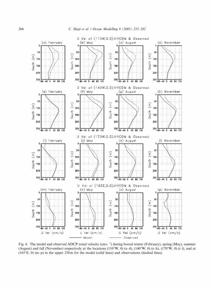
Fig. 6. The model and observed ADCP zonal velocity (cms�1) during boreal winter (February), spring (May), summer
(August) and fall (November) respectively at the locations (110�W, 0) (a–d), (140�W, 0) (e–h), (170�W, 0) (i–l), and at
(165�E, 0) (m–p) in the upper 250m for the model (solid lines) and observations (dashed lines).
266 C. Shaji et al. / Ocean Modelling 9 (2005) 253–282
C. Shaji et al. / Ocean Modelling 9 (2005) 253–282 267
that the simulated flow has a westward bias above 120m from spring through autumn. As a result,the simulated westward nearsurface SEC is stronger, and the simulated EUC core deeper andweaker, than the observed flow. The weaker EUC core velocities simulated by HYCOM hereand at 110�W may also indicate that meridional grid resolution has to be increased to properlysimulate the core velocity maximum. A spring surface flow reversal also occurs at this locationthat is not reproduced by the model. The flow differences at this location and at 110�W suggestthat the surface stress forcing the model has a westward bias, or perhaps that the vertical viscosityprofiles produced by the KPP vertical mixing submodel have errors that adversely affect verticalshear and hence the vertical profile of zonal current produced by the model.
The location 170�W is a transition region between the cold tongue and warm pool. As seen inFig. 6i–l, differences between the model and observed profiles are small at this location. Coredepth of the simulated EUC tends to be slightly deeper than observed during spring and summer,and slightly shallower during the remainder of the year. The location 165�E is in the warm poolregion in the western equatorial Pacific where the zonal currents are not as strong. Fig. 6m–p alsoshow reasonable similarity between simulated and observed profiles. The EUC core is much dee-per here that farther to the east and the simulated EUC does not show a depth bias with respect tothe observed EUC.
4. Circulation in the tropical Atlantic Ocean
The surface and subsurface circulation features in the tropical Atlantic Ocean are discussed inthis section.
4.1. Surface circulation
Like the tropical Pacific Ocean, the Atlantic surface circulation is comprised of alternatingbands of westward and eastward flowing zonal currents driven primarily by trade wind forcing.Fig. 7a and b show the simulated currents and temperature at 15m depth during February andAugust. Fig. 7c and d show the currents and temperature during February and August fromthe satellite-tracked drifters. Comparisons are more difficult in the tropical Atlantic due to largespatial data gaps in the observations. Both the model and observations show the major surfacezonal currents such as the westward flowing SEC and NEC and the eastward flowing NECC.The SEC is strongest within a few degrees of the equator. Most of this flow feeds the North BrazilCurrent (NBC) and contributes in part to the northward transport of the upper limb of the Atlan-tic meridional overturning circulation (Halliwell et al., 2003). The NEC, usually present north of10�N, is a comparatively weak, predominantly zonal flow in both the simulation and observa-tions. The model reproduces the seasonal appearance and disappearance of the NECC (Garzoliand Katz, 1983; Richardson and Walsh, 1986). Similar to the tropical Pacific Ocean, the simulatedcurrents more than several degrees away from the equator are generally weaker than observedcurrents, again due in part to the lower resolution there.
In both the simulation and observations, the strongest flow is associated with the NBC. DuringFebruary, the simulated and observed NBC both attain a maximum speed of about 80cms�1.During August, both observed and simulated maximum speeds reach about 100cms�1. During
(a) (b)
(c) (d)
Fig. 7. The simulated currents and temperature at 15m depth for (a) February and (b) August, and the satellite-tracked
drifter currents and temperature for (c) February and (d) August, for the tropical Atlantic Ocean. The current vectors
(cms�1) are superimposed on the color temperature image (�C).
268 C. Shaji et al. / Ocean Modelling 9 (2005) 253–282
February, the NECC is a weak flow at 5�N east of 25�W in both simulations and observations.During August, the NECC is strong across the entire basin, with the retroflection of the NBC sup-plying water to this current (Garzoli and Katz, 1983). The NECC continues its journey towardsthe east into the Gulf of Guinea as the Guinea Current, where it is prevented from flowing northby the African coastline and thus turns south to feed the SEC. The model faithfully reproduces theseasonal variability of this equatorial gyre structure and is also in realistic accord with othermodel simulations, such as that of Murtugudde et al. (1995, 1996) and Philander and Pacanowski(1986). Neither the simulation nor the observations show the SECC during February and August.Equatorial divergence is evident in both simulation and observations, and is stronger in August(Fig. 7b and d) due to stronger trade winds.
Observed and simulated temperature distributions correspond well during both February andAugust. During boreal summer, the northern tropical Atlantic is mainly occupied by warm water.In the Intra-Americas Sea, the temperature exceeds 28�C, and represents the eastern part of theWestern Hemisphere warm pool (Wang and Enfield, 2001, 2003). During summer, the equatorialcold tongue resulting from equatorial upwelling exists in the east-central Atlantic. It is difficult todetermine the fidelity with which the simulation reproduces the cold tongue because it is poorlyresolved by the observations. Comparing the few observational grid boxes in the cold tongueto the corresponding observational grid boxes suggests that model 15m temperature is equal toor colder than the observed temperature. The temperature distribution in the South Atlanticshows some similarities with the South Pacific Ocean. In particular, marked differences from zonal
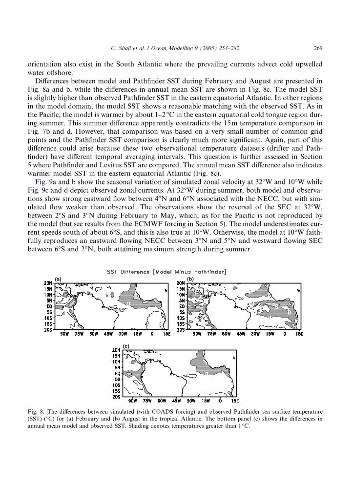
C. Shaji et al. / Ocean Modelling 9 (2005) 253–282 269
orientation also exist in the South Atlantic where the prevailing currents advect cold upwelledwater offshore.
Differences between model and Pathfinder SST during February and August are presented inFig. 8a and b, while the differences in annual mean SST are shown in Fig. 8c. The model SSTis slightly higher than observed Pathfinder SST in the eastern equatorial Atlantic. In other regionsin the model domain, the model SST shows a reasonable matching with the observed SST. As inthe Pacific, the model is warmer by about 1–2 �C in the eastern equatorial cold tongue region dur-ing summer. This summer difference apparently contradicts the 15m temperature comparison inFig. 7b and d. However, that comparison was based on a very small number of common gridpoints and the Pathfinder SST comparison is clearly much more significant. Again, part of thisdifference could arise because these two observational temperature datasets (drifter and Path-finder) have different temporal averaging intervals. This question is further assessed in Section5 where Pathfinder and Levitus SST are compared. The annual mean SST difference also indicateswarmer model SST in the eastern equatorial Atlantic (Fig. 8c).
Fig. 9a and b show the seasonal variation of simulated zonal velocity at 32�W and 10�W whileFig. 9c and d depict observed zonal currents. At 32�W during summer, both model and observa-tions show strong eastward flow between 4�N and 6�N associated with the NECC, but with sim-ulated flow weaker than observed. The observations show the reversal of the SEC at 32�W,between 2�S and 3�N during February to May, which, as for the Pacific is not reproduced bythe model (but see results from the ECMWF forcing in Section 5). The model underestimates cur-rent speeds south of about 6�S, and this is also true at 10�W. Otherwise, the model at 10�W faith-fully reproduces an eastward flowing NECC between 3�N and 5�N and westward flowing SECbetween 6�S and 2�N, both attaining maximum strength during summer.
(a) (b)
(c)
Fig. 8. The differences between simulated (with COADS forcing) and observed Pathfinder sea surface temperature
(SST) (�C) for (a) February and (b) August in the tropical Atlantic. The bottom panel (c) shows the differences in
annual mean model and observed SST. Shading denotes temperatures greater than 1 �C.

(a) (b)
(c) (d)
Fig. 9. Seasonal variations of the simulated zonal surface current along (a) 32�W and (b) 10�W. Seasonal variations of
the observed satellite-tracked drifter zonal surface current along (c) 32�W and (d) 10�W. The unit of current is cms�1.
Shading denotes eastward zonal current.
270 C. Shaji et al. / Ocean Modelling 9 (2005) 253–282
4.2. Subsurface circulation
Fig. 10a and b depict the vertical structure of zonal currents in the upper 300m along the equa-tor during February and August. The westward SEC at the surface and the eastward EUC beloware clearly evident while the westward component of the northwestward NBC flow is evident at alldepths at the western end of the basin. In February, the SEC is confined above 30m (Fig. 10a)while in August it strengthens and thickens to 50m (Fig. 10b). Associated with this thickening,the EUC core depth increases. Throughout the year, the EUC is deepest and strongest in the west-ern basin while decelerating and shoaling to the east. In February, the EUC core velocity maxi-mum exceeds 60cms�1 and is located at 35�W at a depth of 100m. Similar to the Pacific, two corevelocity maxima exist in August: one at 30�W, 115m and the other at 38�W, 125m. This simulatedflow structure is in good agreement with previous observational studies (Philander, 1990). Modelstudies have produced EUCs with a wide range of maximum magnitudes, with model resolutionplaying a significant role, making it difficult to evaluate the present simulation. Low-resolutionmodels tend to underestimate the core velocity, such as the 2� MICOM simulation of Chassignet

(a) (b)
(c) (d)
(e) (f)
Fig. 10. Vertical section of simulated zonal current (cms�1) along the equator in the upper 300m of the water column
during (a) February and (b) August for the tropical Atlantic Ocean. Vertical section of simulated temperature (�C)along the equator in the upper 300m of the water column during (c) February and (d) August. Vertical section of the
observed climatological temperature (C) along the equator in the upper 300m of the water column during (e) February
and (f) August for the tropical Atlantic Ocean, obtained from the Levitus climatology. Shading represents eastward
zonal current for velocity (upper panels) and isotherms greater than 20 �C (middle and bottom panels).
C. Shaji et al. / Ocean Modelling 9 (2005) 253–282 271

272 C. Shaji et al. / Ocean Modelling 9 (2005) 253–282
et al. (1996) (core velocity of 30cms�1) and the isopycnic model analysis of Oberhuber (1993)(core velocity of 50cms�1). In higher resolution simulations, Murtugudde et al. (1996) simulatedthe EUC and obtained a maximum core velocity of about 90cms�1 in March while Philander andPacanowski (1986) obtained a core velocity of 90cms�1. Observations tend to support this largervelocity maximum (e.g., Schott et al., 1995, who measured maximum velocity exceeding 80cms�1
at 35�W). The weaker core velocity maximum simulated by HYCOM again suggests that merid-ional resolution must be smaller than 0.5� to properly simulate this maximum.
Fig. 10 (c, d) and (e, f) show the vertical structure of temperature along the equator during Feb-ruary and August obtained from the simulation and from the Levitus climatology. Both the sim-ulated and observed thermoclines slope upward toward the east and have a larger slope insummer. Similar to the tropical Pacific Ocean, the simulated isotherms, and thus the thermocline,are deeper compared to the observed isotherms, in this case provided by the Levitus climatologyinstead of the TAO array. This is again most evident beneath the core of the EUC.
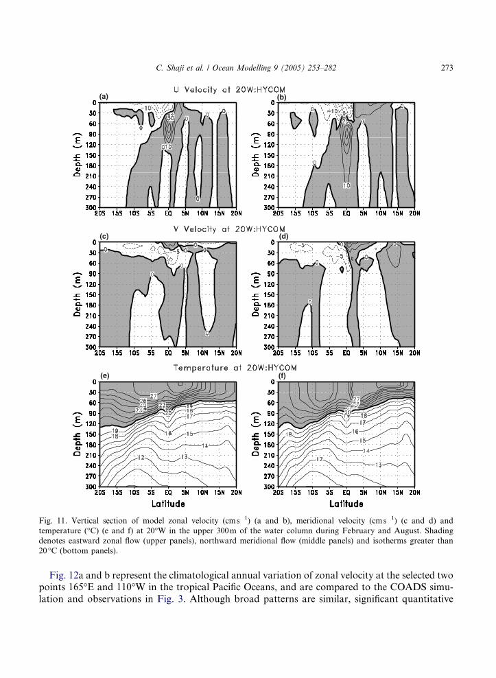
Fig. 11a–f show the vertical sections of zonal velocity, meridional velocity and temperature inthe upper 300m of the Atlantic Ocean at 20�W during February and August. The meridional/ver-tical structure of the flow (Fig. 11a and b) demonstrates that the westward flowing SEC is con-fined above 30m within 5�S–3�N and exists as a thinner, weaker westward flow south of 5�S.The SEC intensifies in August between 5�S and 3�N, as does the eastward flowing NECC fartherto the north. The EUC is confined between 2�S and 2�N as it is in the Pacific. During February,the EUC is confined between 30 and 130m, with a core velocity exceeding 40cms�1 at 80m. InAugust, the vertical extent of the EUC below 30m expands substantially while the core velocityexceeds 40cms�1 at 90m. The vertical structure of meridional velocity at 20�W (Fig. 11c and d)shows clear evidence of surface divergence near the equator during summer only, which is strong-est between the surface and 90m. There is no clear evidence of the expected quasi-geostrophicmeridional convergence below. During winter, surface meridional divergence is only evident inthe upper 10m and is centered near 1�S. As for summer, there is no clear evidence of the expectedquasi-geostrophic meridional convergence below on the equator.
The vertical structure of temperature at 20�W (Fig. 11e and f) generally shows the classical pat-tern that was observed in the Pacific (Fig. 5e and f) and inferred from earlier studies (Philander,1990). The shallower thermocline near the equatorial is evident, but the seasonal cycle of thetrough-ridge system north of the equator associated with the NECC is weak because this sectionis located to the east of the strongest part of the NECC. The upward (downward) bowing of iso-therms above (below) the EUC core within 2� of the equator that reflects the equatorial quasi-geostrophic balance associated with the EUC and the SEC jet above (Philander, 1990) is not asstrong in the Atlantic as in the Pacific.
5. Sensitivity studies
The simulations presented in Sections 3 and 4 were driven by the COADS monthly climato-logical surface forcing fields. In this section, we deal with model sensitivity to the forcing. Forthat, we performed another simulation identical to the COADS simulation except that it was dri-ven by surface forcing fields obtained from the ECMWF ERA-15 reanalysis climatology. TheECMWF results are presented separately for the Pacific and Atlantic Oceans.
(a) (b)
(c) (d)
(e) (f)
Fig. 11. Vertical section of model zonal velocity (cms�1) (a and b), meridional velocity (cms�1) (c and d) and
temperature (�C) (e and f) at 20�W in the upper 300m of the water column during February and August. Shading
denotes eastward zonal flow (upper panels), northward meridional flow (middle panels) and isotherms greater than
20 �C (bottom panels).
C. Shaji et al. / Ocean Modelling 9 (2005) 253–282 273
Fig. 12a and b represent the climatological annual variation of zonal velocity at the selected twopoints 165�E and 110�W in the tropical Pacific Oceans, and are compared to the COADS simu-lation and observations in Fig. 3. Although broad patterns are similar, significant quantitative
(a) (b)
Fig. 12. Seasonal variations of the simulated zonal surface current along (a) 165�E and (b) 110�W based on the
simulation with ECMWF forcing. The unit of current is cms�1, and shading denotes eastward zonal flow. These figures
can be compared with those from the COADS simulation (Fig. 3a and b) and those from the observed drifter data (Fig.
3c and d).
274 C. Shaji et al. / Ocean Modelling 9 (2005) 253–282
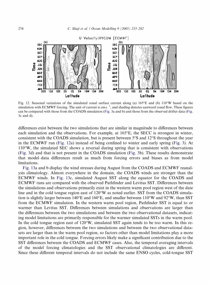
differences exist between the two simulations that are similar in magnitude to differences betweeneach simulation and the observations. For example, at 165�E, the SECC is strongest in winter,consistent with the COADS simulation, but is present between 5�S and 12�S throughout the yearin the ECMWF run (Fig. 12a) instead of being confined to winter and early spring (Fig. 3). At110�W, the simulated SEC shows a reversal during spring that is consistent with observations(Fig. 3d) and that is not present in the COADS simulation (Fig. 3b). These results demonstratethat model–data differences result as much from forcing errors and biases as from modellimitations.
Fig. 13a and b display the wind stresses during August from the COADS and ECMWF reanal-ysis climatology. Almost everywhere in the domain, the COADS winds are stronger than theECMWF winds. In Fig. 13c, simulated August SST along the equator for the COADS andECMWF runs are compared with the observed Pathfinder and Levitus SST. Differences betweenthe simulations and observations primarily exist in the western warm pool region west of the dateline and in the cold tongue region east of 120�W as noted earlier. SST from the COADS simula-tion is slightly larger between 140�E and 160�E, and smaller between 110�W and 92�W, than SSTfrom the ECMWF simulation. In the western warm pool region, Pathfinder SST is equal to orwarmer than Levitus SST. Differences between simulations and observations are larger thanthe differences between the two simulations and between the two observational datasets, indicat-ing model limitations are primarily responsible for the warmer simulated SSTs in the warm pool.In the cold tongue region east of 120�W, simulated SST again tends to be too warm. In this re-gion, however, differences between the two simulations and between the two observational data-sets are larger than in the warm pool region, so factors other than model limitations play a moreimportant role in the cold tongue. Forcing errors likely make a significant contribution due to theSST differences between the COADS and ECMWF cases. Also, the temporal averaging intervalsof the model forcing climatologies and the SST observational climatologies are different.Since these different temporal intervals do not include the same ENSO cycles, cold-tongue SST
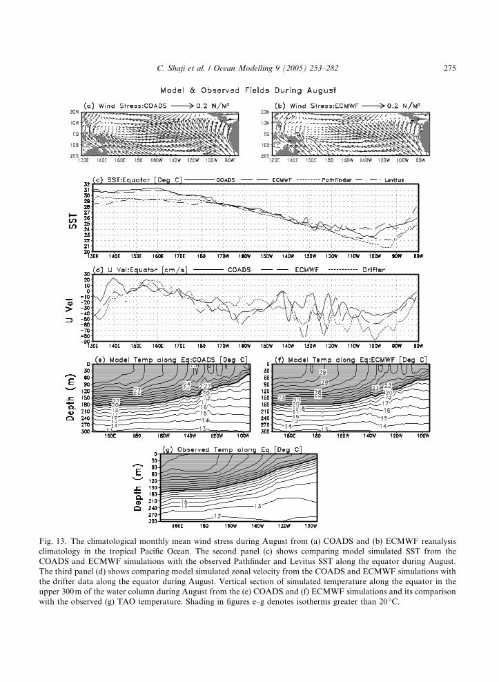
Fig. 13. The climatological monthly mean wind stress during August from (a) COADS and (b) ECMWF reanalysis
climatology in the tropical Pacific Ocean. The second panel (c) shows comparing model simulated SST from the
COADS and ECMWF simulations with the observed Pathfinder and Levitus SST along the equator during August.
The third panel (d) shows comparing model simulated zonal velocity from the COADS and ECMWF simulations with
the drifter data along the equator during August. Vertical section of simulated temperature along the equator in the
upper 300m of the water column during August from the (e) COADS and (f) ECMWF simulations and its comparison
with the observed (g) TAO temperature. Shading in figures e–g denotes isotherms greater than 20 �C.
C. Shaji et al. / Ocean Modelling 9 (2005) 253–282 275

276 C. Shaji et al. / Ocean Modelling 9 (2005) 253–282
simulated by the model and mean SST from the observational datasets will differ to some extenteven if a perfect model is used.
Fig. 13d shows the simulated zonal velocity at 15m depth along the equator during Augustfrom the COADS and ECMWF simulations, and also from the drifter data, revealing the west-ward-flowing SEC east of 175�E. In general, differences between the simulations are as large asdifferences between each simulation and the observations. Simulated westward zonal velocityassociated with the SEC is generally smaller than observed zonal velocity east of 120�W. Fig.13e and f show vertical sections of simulated temperature along the equator during August fromthe COADS and ECMWF forcing while Fig. 13g shows the observed TAO temperature along theequator during August. In general, the isotherms from the ECMWF simulation are slightly deepercompared to the COADS simulation, and thus slightly less realistic compared to observations.The COADS run produces a thermocline with a larger upward slope toward the east that is closerto observations (Fig. 13g).
For the Atlantic, Fig. 14a and b show the climatological annual variation of zonal velocitysimulated with ECMWF forcing at 32�W and 10�W, which are compared to the COADS runand observations in Fig. 9. Although broad patterns are similar as they were in the Pacific, sig-nificant quantitative differences exist between the two simulations that are again similar in mag-nitude to differences between each simulation and the observations. For example, at 32�W, thespring reversal of the SEC at the equator is more clearly evident in the ECMWF simulation (Fig.14a) as compared to the COADS run (Fig. 9a), and this reversal is more consistent with theobservations (Fig. 9c). The ECMWF forcing generated a stronger SEC during summer at10�W (Fig. 14b) compared to the COADS simulation (Fig. 9b), the latter being closer to obser-vations (Fig. 9d).
Fig. 15a and b display wind stresses during August from the COADS and ECMWF climatol-ogies. As in the Pacific Ocean, the COADS winds are stronger compared to the ECMWF winds.The simulated SST along the equator during August for the COADS and ECMWF runs, along
(a) (b)
Fig. 14. Seasonal variations of the simulated zonal surface current along (a) 32�W and (b) 10�W based on the
simulation with ECMWF forcing. The unit of current is cms�1, and shading denotes eastward zonal flow. These figures
can be compared with those from the COADS simulation (Fig. 9a and b) and those from the observed drifter data (Fig.
9c and d).
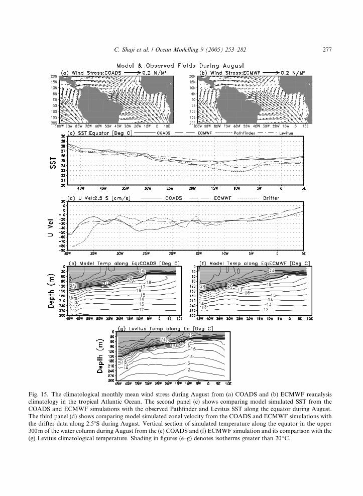
Fig. 15. The climatological monthly mean wind stress during August from (a) COADS and (b) ECMWF reanalysis
climatology in the tropical Atlantic Ocean. The second panel (c) shows comparing model simulated SST from the
COADS and ECMWF simulations with the observed Pathfinder and Levitus SST along the equator during August.
The third panel (d) shows comparing model simulated zonal velocity from the COADS and ECMWF simulations with
the drifter data along 2.5�S during August. Vertical section of simulated temperature along the equator in the upper
300m of the water column during August from the (e) COADS and (f) ECMWF simulation and its comparison with the
(g) Levitus climatological temperature. Shading in figures (e–g) denotes isotherms greater than 20 �C.
C. Shaji et al. / Ocean Modelling 9 (2005) 253–282 277
278 C. Shaji et al. / Ocean Modelling 9 (2005) 253–282
with the observed Pathfinder and Levitus SST, are shown in Fig. 15c. Both the COADS andECMWF simulations reveal zonal oscillations of SST along the equator. These oscillationsmay result from the existence of tropical instability wave variability. West of 30�W, SST fromthe COADS run is slightly warmer than observations while SST from the ECMWF run is slightlycolder. East of 13�W, simulated SST is warmer than observed. East of 30�W, Levitus SST is war-mer than Pathfinder, with the difference exceeding 1�C near 15�W. As for the Pacific Ocean, bothforcing biases and differences in the temporal averaging intervals of the model forcing and SSTclimatology contribute to the SST differences in the Atlantic cold tongue region. However, modellimitations also contribute to SST errors in the cold tongue, probably resulting in part from thetendency of HYCOM to produce a thermocline that is too deep in the eastern equatorial region,as was also the case in the Pacific.
The zonal flow along 2.5�S during August at 15m depth simulated with the COADS andECMWF forcing are compared with the drifter data at 15m depth (Fig. 15d). This latitude is cho-sen because of the poor observational sampling along the equator (Fig. 7). East of 15�W, the SECmagnitude in both simulations compare favorably to each other and to observations. However,these agreements are not as good west of 15�W. West of 35�W, the magnitude of SEC is higherthan the simulations. Fig. 15d also reveals zonal oscillations in the zonal flow field along 2.5�S inboth simulations. This can also be due to the effect of tropical instability wave variability. Thevertical structure of temperature along the equator during August from the COADS andECMWF simulations (Fig. 15e and f) are compared with the Levitus temperature (Fig. 15g).As for the Pacific, the COADS simulation produces a slightly shallower thermocline than theECMWF simulation, with the shallower depth being in closer agreement with climatology.
This two-ocean comparison between two simulations driven by different climatological forcingsets demonstrates that forcing accuracy can be as important as model limitations in producingerrors and biases in simulated fields, making it difficult to judge standalone model performance.Although some aspects of the ECMWF simulation were superior, such as the spring SEC reversalat the equator in both the Atlantic and Pacific Oceans, careful evaluation of the three-dimensionaltemperature and flow structures convinced us that the COADS simulation was closer to observa-tions in more respects than the ECMWF simulation, particularly in regards to SST and subsur-face thermal fields.
6. Summary
The purpose of this study was to evaluate capabilities and limitations of a new ocean model(HYCOM) configured on a non-uniform horizontal grid spanning 30�S–65.5�N and 102�E–15�E to simulate the climatological annual cycle of the tropical Pacific and Atlantic Oceans.Monthly climatological surface fields obtained from the COADS data are used to drive the pri-mary simulation. Sensitivity to forcing is considered by comparing the primary COADS simula-tion to another driven by the ECMWF ERA-15 monthly reanalysis climatology that is otherwiseidentical to the primary simulation. The upper-ocean currents, temperature and many features ofthe tropical ocean thermocline are in general realistically modeled. One goal was to evaluate theuse of latitude dependent meridional resolution that provides enhanced resolution near the equa-tor (0.72� zonal by 0.36� meridional). The importance of enhanced resolution is evident because
C. Shaji et al. / Ocean Modelling 9 (2005) 253–282 279
HYCOM substantially underestimated zonal current magnitudes away from the equator whereboth zonal and meridional resolution was low.
In the Pacific Ocean, the presence and seasonality of the major surface zonal currents such asthe SEC, NEC, NECC and SECC are in good correspondence with the observations. Both modeland drifter velocities show the SEC accelerating along the equator from east to west, with merid-ional divergence associated with equatorial upwelling present all year but strongest in summer.Analysis of the annual cycle of zonal equatorial currents discloses a spring reversal of the SECat 110�W in the observations. The COADS simulation does not reproduce this reversal, butthe ECMWF does (albeit too weak). The occurrence and seasonality of the EUC has been veryrealistically modeled except for the tendency of the core velocity to be somewhat too weak,and also the fact that the simulated EUC terminates a few degrees farther to the west than ob-served. Insufficient meridional resolution could contribute to both of these shortcomings. Themodel also reproduces zonal and meridional slopes, ridges, and troughs in the thermocline,including their strong seasonal variations. Both the modeled and observed thermal structureshows a fairly strong thermocline along the equator, with a downward slope towards the west.The depth of the equatorial thermocline tends to be slightly deeper than observed. The model gen-erally does a good job in simulating the seasonal evolution of off-equatorial zonal currents asso-ciated with the thermocline ridges and troughs except for the tendency to underestimatemagnitudes. The warm and cold water regions and their seasonality in the tropical Pacific hasbeen realistically simulated by the model and is in good agreement with the drifter data. A com-parison of simulated SST with the observed SST climatologies reveals that simulated SST is war-mer than the observations in the eastern equatorial cold tongue and in the warm pool waters ofthe western Pacific and also the eastern Pacific (the western limb of the Western Hemisphere warmpool). The temperature difference in the warm pool regions is similar no matter which observedtemperature climatology is used for the comparison, indicating that model biases are the primaryproblem. The magnitude of the temperature difference in the cold tongue varies depending on thetemperature climatology used for the comparison. This indicates that the different temporal aver-aging intervals used for these climatologies, which can differ from the temporal averaging intervalof the atmospheric forcing climatologies used to drive the model, contribute in part to the coldtongue temperature differences (i.e., they are averaged over different sets of ENSO events).
In the tropical Atlantic Ocean, the model captured all the major currents such as the SEC,NEC, NECC and NBC. The highest current speeds are observed in the NBC in both the simula-tion and drifter velocity climatology. During winter, NECC is weak and mainly concentrated inthe eastern equatorial Atlantic Ocean. During summer, this current is intensified and is suppliedby the retroflection of the NBC around 5�N. The SEC indicates divergence at the equator, whichis quite strong during summer and enhances the equatorial upwelling at this time. At 32�W, thedrifter data shows the spring reversal of the SEC near the equator. As for the Pacific, this reversalwas present in the HYCOM simulation driven by ECMWF (albeit too weak), but not in the sim-ulation driven by COADS. As for the Pacific, the simulated EUC tends to be a little too deep andtoo slow, with resolution again probably contributing to the underestimate of core velocity mag-nitude. The simulated surface warm pool and cold tongue areas and their seasonal changes in thetropical Atlantic Ocean are generally in good agreement with the drifter temperature climatology.The temperature distribution in the Atlantic Ocean shows some similarities with the PacificOcean, particularly south of the equator where surface temperatures are much the same in both
280 C. Shaji et al. / Ocean Modelling 9 (2005) 253–282
the oceans. As for the Pacific, model SST is slightly warmer in the eastern equatorial cold tongue.The temporal averaging interval of the climatology used for the comparison is again a factor inthe magnitude of the observed–simulated temperature difference. The tendency for isotherms tobe too deep at the equator is larger in the Atlantic than in the Pacific. This problem could be re-lated to too much vertical mixing, or could result from water with the wrong temperature con-verging toward the equator at depth. If the latter is true, then model biases off the equatorcontribute to the observed equatorial biases.
Differences in the circulation pattern and temperature distribution in the tropical Pacific andAtlantic Oceans arising from the use of ECMWF forcing were documented. In addition to thespring SEC reversal differences mentioned above, the simulation with the ECMWF forcingshowed the presence of the SECC in the western Pacific throughout the year, with its peak occur-ring during winter. The ECMWF simulation generated higher SST in the eastern equatorial Pa-cific compared to the COADS simulation. A comparison of equatorial zonal flow in the PacificOcean from the two simulations showed marked differences, especially in the east-central andwestern equatorial regions. The isotherms are deeper in the ECMWF forcing simulation. In boththe tropical Pacific and Atlantic Oceans, the COADS surface wind stress is stronger than theECMWF wind stress. In contrast, SST and subsurface temperatures in the COADS case com-pared more favorably to observations, leading us to choose the COADS case as the primaryexperiment. Overall, model performance is encouraging, and we anticipate that future experi-ments conducted with different vertical mixing choices, different vertical coordinate choices, dif-ferent horizontal advection schemes, and modifications in other model subgrid-scaleparameterizations, in conjunction with improved high-frequency forcing, will produce substan-tially improved simulations.
Acknowledgments
This work was supported by a grant from the NOAA Office of Global Programs and by NOAAEnvironmental Research Laboratories through their base funding of Atlantic Oceanographic andMeteorological Laboratory (AOML). We are so thankful to Dr. R. Lumpkin (CIMAS, Univer-sity of Miami) for drifter data and Dr. M.J. McPhaden (Pacific Marine Environmental Labora-tory) for TAO array data. The constructive comments and suggestions made by two anonymousreviewers and the suggestions from Editor Peter Killworth helped us to improve the manuscript.
References
Bleck, R., 2002. An oceanic general circulation model framed in hybrid isopycnic-Cartesian coordinates. Ocean Modell.
4, 55–88.
Busalacchi, A.J., O�Brien, J.J., 1980. The seasonal variability in a model of the tropical Pacific. J. Phys. Oceanogr. 10,
1929–1951.
Casey, K.S., Cornillon, P., 1999. A comparison of satellite and in situ based sea surface temperature climatologies. J.
Climate 12, 1848–1863.
Chassignet, E.P., Smith, L.T., Halliwell, G.R., Bleck, R., 2003. North Atlantic Simulations with the Hybrid Coordinate
Ocean Model (HYCOM): impact of the vertical coordinate choice, reference density, and thermobaricity. J. Phys.
Oceanogr. 33, 2504–2526.

C. Shaji et al. / Ocean Modelling 9 (2005) 253–282 281
Chassignet, E.P., Smith, L.T., Bleck, R., Bryan, F.O., 1996. A model comparison: numerical simulations of the
north and equatorial Atlantic oceanic circulation in depth and isopycnic coordinates. J. Phys. Oceanogr. 26, 1849–
1867.
Chen, D., Rothstein, L., Busalacchi, A., 1994. A hybrid vertical mixing scheme and its application to tropical ocean
models. J. Phys. Oceanogr. 24, 2156–2179.
Cox, M.D., 1984 A primitive equation three-dimensional model of the ocean. NOAA Tech. Rep. 1, GFDL/NOAA,
Princeton University, NJ, 144pp.
Evans, R., Podesta, G., 1996. AVHRR pathfinder SST approach and results. EOS 77 (46).
Garzoli, S.L., Katz, E.J., 1983. The forced annual reversal of the Atlantic North Equatorial Countercurrent. J. Phys.
Oceanogr. 13, 2082–2090.
Gibson, J.K., Kallberg, P., Uppala, S., Hernandez, A., Nomura, A., Serrano, E., 1999: ECMWF Re-analysis Project
Report Series: 1. ERA-15 Description (version 2—January 1999). ECMWF. Reading, Berkshire, UK, 77pp.
Halliwell Jr., G.R., 2004. Evaluation of vertical coordinate and vertical mixing algorithms in the Hybrid-Coordinate
Ocean Model (HYCOM). Ocean Modell. 7, 285–322.
Halliwell Jr., G.R., Weisberg, R.H., Mayer, D.A., 2003. A synthetic float analysis of upper-limb meridional overturning
circulation interior ocean pathways in the tropical/subtropical Atlantic Ocean. In: Goni, G., Malanotte-Rizzoli, P.
(Eds.), Interhemispheric Water Exchange in the Atlantic. Elsevier Publishing Company, pp. 93–136.
Langlois, G., Brydon, D., Bleck, R., Dean, S., 1997. Miami Isopycnic Coordinate Ocean Model (MICOM) User�sManual.
Large, W.G., Mc Williams, J.C., Doney, S.C., 1994. Oceanic vertical mixing: review and a model with a nonlocal
boundary layer parameterization. Rev. Geophys. 32, 363–403.
Levitus, S., Boyer, T., 1994. World Ocean Atlas 1994, Volume 4: Temperature. NOAA Atlas NESDIS 4. US Dept. of
Commerce, Washington, DC.
Levitus, S., Burgett, R., Boyer, T., 1994. World Ocean Atlas 1994, Volume 3: Salinity. NOAA Atlas NESDIS 3. US
Dept. of Commerce, Washington, DC.
Lu, P., McCreary, J.P., Klinger, B.A., 1998. Meridional circulation cells and the source waters of the Pacific equatorial
undercurrent. J. Phys. Oceanogr. 28, 62–84.
Lumpkin, R., 2003. Decomposition of surface drifter observations in the Atlantic Ocean. Geophys. Res. Lett. 30, 14,
doi:10.1029/2003GL017519.
McPhaden, M.J., et al., 1998. The Tropical Ocean Global Atmosphere (TOGA) observing system: a decade of
progress. J. Geophys. Res. 103, 14169–14240.
Mellor, G.L., Yamada, T., 1982. Development of a turbulence closure model for geophysical fluid problems. Rev.
Geophys. Space Phys. 20, 851–875.
Murtugudde, R., Cane, M., Prasad, V., 1995. A reduced gravity, primitive equation, isopycnal ocean GCM:
formulation and simulations. Mon. Weather Rev. 123, 2864–2887.
Murtugudde, R., Seager, R., Busalacchi, A., 1996. Simulation of the tropical oceans with an ocean GCM coupled to an
Atmospheric Mixed Layer Model. J. Climate 9, 1795–1815.
Niiler, P., 2001. The world ocean surface circulation. In: Siedler, G., Church, J., Gould, J. (Eds.), Ocean Circulation
and Climate, International Geophysics Series 77. Academic Press.
Niiler, P.P., Kraus, E.B., 1977. One-dimensional models of the upper ocean. In: Kraus, E.B. (Ed.), Modelling and
Prediction of the Upper Layers of the Ocean. Pergamon, New York, pp. 143–172.
Oberhuber, J., 1993. Simulation of the Atlantic circulation with a coupled sea ice-mixed layer-isopycnal general
circulation model, part II: model experiment. J. Phys. Oceanogr. 17, 1986–2002.
Philander, S.G., 1990. El Nino, La Nina, and the Southern Oscillation. Academic Press Inc., San Diego, California,
293pp.
Philander, S.G., Pacanowski, R., 1986. A model of the seasonal cycle in the tropical Atlantic Ocean. J. Geophys. Res.
91, 14192–14206.
Philander, S.G., Hurlin, W., Seigel, A., 1987. Simulation of the seasonal cycle of the tropical Pacific Ocean. J. Phys.
Oceanogr. 17, 1986–2002.
Price, J.F., Weller, R.A., Pinkel, R., 1986. Diurnal cycling: observations and models of the upper ocean response to
diurnal heating, cooling and wind mixing. J. Geophys. Res. 91, 8411–8427.
282 C. Shaji et al. / Ocean Modelling 9 (2005) 253–282
Richardson, P.L., Walsh, D., 1986. Mapping climatological seasonal variations of the surface currents in the tropical
Atlantic using ship drifts. J. Geophys. Res. 91, 10537–10550.
Schott, F.A., Stramma, L., Fischer, J., 1995. The warm water inflow into the western tropical Atlantic boundary
regime, spring 1994. J. Geophys. Res. 100, 24745–24760.
Sun, S., Bleck, R., Rooth, C., Dukowicz, J., Chassignet, E., Killworth, P., 1999. Inclusion of thermobaricity in
isopycnic-coordinate ocean models. J. Phys. Oceanogr. 29, 2719–2729.
Tomczak, M., Godfrey, J.S., 1994. Regional Oceanography: An Introduction. Pergamon, 422pp.
Turner, J.S., Kraus, E.B., 1967. A one-dimensional model of the seasonal thermocline II: the general theory and its
consequences. Tellus 18, 98–105.
Wang, C., Enfield, D.B., 2001. The tropical Western Hemisphere warm pool. Geophys. Res. Lett. 28, 1635–1638.
Wang, C., Enfield, D.B., 2003. A further study of the tropical Western Hemisphere warm pool. J. Climate 16, 1476–
1493.
Woodruff, S.D., Sultz, R.J., Jenne, R.L., Steurer, P.M., 1987. A comprehensive ocean-atmosphere data set. Bull. Amer.
Meteor. Soc. 68, 1239–1250.
Yu, X., McPhaden, M.J., 1999. Seasonal variability in the equatorial Pacific. J. Phys. Oceanogr. 29, 925–947.