simulation of the performance of ieee 802.16-2004 fixed...
TRANSCRIPT

Simulation of the Performance of IEEE
802.16-2004 Fixed Broadband Wireless
Access Technology
by
Saideepthi Katragunta
Problem report submitted to theCollege of Engineering and Mineral Resources
at West Virginia Universityin partial fulfillment of the requirements
for the degree of
Master of Sciencein
Electrical Engineering
Matthew C.Valenti, Ph.D., ChairBrian D.Woerner, Ph.D., Co-Chair
Natalia A.Schmid, Ph.D.
Lane Department of Computer Science and Electrical Engineering
Morgantown, West Virginia2007
Keywords: Broadband wireless access, MIMO, space time codes, turbo codes
Copyright 2007 Saideepthi Katragunta

Abstract
Simulation of the Performance of IEEE 802.16-2004 Fixed Broadband Wireless AccessTechnology
by
Saideepthi KatraguntaMaster of Science in Electrical Engineering
West Virginia University
Matthew C.Valenti, Ph.D., Chair
The explosive growth of the Internet over the last decade has led to an increasing demand forhigh-speed, ubiquitous Internet access. Fixed broadband wireless access (BWA) is an idealsolution for providing high data rate communications, where traditional wireline technolo-gies like digital subscriber line (DSL) and cable modems are either unavailable or too costlyto be installed. IEEE 802.16-2004, also known as WiMax, is a standard that promotes thedeployment of fixed broadband wireless access. To achieve this, the IEEE 802.16-2004 stan-dard specifies three air interfaces which include WirelessMAN-SCa, WirelessMAN-OFDM,and WirelessMAN-OFDMA to operate in a non-line-of-sight (NLOS) environment withinthe licensed frequencies below 11 GHz.
In this project, we simulate the performance of the WirelessMAN-SCa option of theIEEE 802.16-2004 standard. First we provide an overview of the physical layer features andthe channel model of a WiMax system. We show the advantages of using multiple-input-multiple-output (MIMO) techniques to combat the fading effects in a wireless channel. Thedesign of a convolutional turbo code (CTC), used as an optional error correction technique byIEEE 802.16-2004 is described. For the Alamouti space time block code (STBC), consideringthe two transmit and one receive antenna case, we derive the equations for the log likelihoodratios (LLRs) to be given as inputs to the CTC decoder. STBC gives diversity gain, CTCgives coding gain, and a concatenation of both STBC and CTC simultaneously achievesdiversity and coding gain.
iii
Acknowledgments
I am very grateful to Dr. Brian Woerner for giving me an opportunity to do research
and for suggesting me this excellent topic to work on. I can undoubtedly say he is one of
the best persons I have known. My sincere thanks to Dr. Matthew Valenti for agreeing to
be my advisor and guiding me through the entire sequence of my Problem report. I admire
his work and talent. His suggestions were of such great help. I thank Dr. Natalia Schmid
for being my committee member and supporting me.
I would like to thank all my friends for making my life at WVU so easy and memorable.
Finally, I would like to thank my dad K. Rajendra Prasad, mom K.Vijaya Lakshmi and my
brother K. Hari Krishna. Whatever I achieve in my life is due to their love and support.

iv
Contents
Acknowledgments iii
List of Figures vi
1 Introduction to Broadband Technology 11.1 Report Outline . . . . . . . . . . . . . . . . . . . . . . . . . . . . . . . . . . 3
2 WiMax System Overview 52.1 Standards for Fixed Broadband Wireless Access . . . . . . . . . . . . . . . . 5
2.1.1 Frequency Band 10-66 GHz . . . . . . . . . . . . . . . . . . . . . . . 52.1.2 Frequency Bands 11 GHz and Below . . . . . . . . . . . . . . . . . . 6
2.2 WirelessMAN-SCa Physical Layer . . . . . . . . . . . . . . . . . . . . . . . . 72.3 Digital Modulation Schemes . . . . . . . . . . . . . . . . . . . . . . . . . . . 8
2.3.1 Representation of Communication Signals . . . . . . . . . . . . . . . 82.3.2 M-ary Phase Shift Keying (MPSK) . . . . . . . . . . . . . . . . . . . 92.3.3 Constellation Mapping . . . . . . . . . . . . . . . . . . . . . . . . . . 10
2.4 Wireless Channel . . . . . . . . . . . . . . . . . . . . . . . . . . . . . . . . . 112.4.1 Rayleigh Fading Distribution . . . . . . . . . . . . . . . . . . . . . . 122.4.2 Block Fading . . . . . . . . . . . . . . . . . . . . . . . . . . . . . . . 132.4.3 Performance of BPSK and QPSK . . . . . . . . . . . . . . . . . . . . 13
2.5 Summary . . . . . . . . . . . . . . . . . . . . . . . . . . . . . . . . . . . . . 14
3 Multiple Antenna Systems 163.1 Introduction to Diversity . . . . . . . . . . . . . . . . . . . . . . . . . . . . . 16
3.1.1 Diversity Combining Techniques . . . . . . . . . . . . . . . . . . . . . 173.2 MIMO Techniques . . . . . . . . . . . . . . . . . . . . . . . . . . . . . . . . 21
3.2.1 Space-Time Block Codes . . . . . . . . . . . . . . . . . . . . . . . . . 223.2.2 Space-Time Trellis Coding . . . . . . . . . . . . . . . . . . . . . . . . 273.2.3 BLAST Techniques . . . . . . . . . . . . . . . . . . . . . . . . . . . . 27
3.3 Summary . . . . . . . . . . . . . . . . . . . . . . . . . . . . . . . . . . . . . 30
4 Turbo Coding for WiMax 314.1 Channel Coding for WiMax-IEEE 802.16-2004 . . . . . . . . . . . . . . . . . 314.2 The need for Channel Coding . . . . . . . . . . . . . . . . . . . . . . . . . . 314.3 Convolutional Turbo Coder . . . . . . . . . . . . . . . . . . . . . . . . . . . 33

CONTENTS v
4.3.1 Introduction . . . . . . . . . . . . . . . . . . . . . . . . . . . . . . . . 334.3.2 CTC Encoder . . . . . . . . . . . . . . . . . . . . . . . . . . . . . . . 334.3.3 CTC Interleaver . . . . . . . . . . . . . . . . . . . . . . . . . . . . . . 354.3.4 CTC Puncturer . . . . . . . . . . . . . . . . . . . . . . . . . . . . . . 36
4.4 CTC Decoder . . . . . . . . . . . . . . . . . . . . . . . . . . . . . . . . . . . 374.4.1 Calculation of the input LLRs to the decoder . . . . . . . . . . . . . 37
4.5 Summary . . . . . . . . . . . . . . . . . . . . . . . . . . . . . . . . . . . . . 40
5 Results and Conclusions 415.1 Performance of Concatenated STBC and CTC for WiMax . . . . . . . . . . 41
5.1.1 System Model for BWA Applications . . . . . . . . . . . . . . . . . . 415.2 Results . . . . . . . . . . . . . . . . . . . . . . . . . . . . . . . . . . . . . . . 435.3 Conclusions . . . . . . . . . . . . . . . . . . . . . . . . . . . . . . . . . . . . 435.4 Future Work . . . . . . . . . . . . . . . . . . . . . . . . . . . . . . . . . . . . 44
References 47

vi
List of Figures
2.1 WirelessMAN-SCa PHY simulator. . . . . . . . . . . . . . . . . . . . . . . . 72.2 Constellation mapping for BPSK and QPSK with Gray encoding. . . . . . . 112.3 SNR vs BER for BPSK in AWGN and fading. . . . . . . . . . . . . . . . . . 15
3.1 Diversity Combining at the Receiver. . . . . . . . . . . . . . . . . . . . . . . 183.2 Bit error rate of BPSK (lower curve) and QPSK (higher curve) in a fading
channel for L = 1, 2, 3 with MRC decoding . . . . . . . . . . . . . . . . . . 203.3 Alamouti space time block code with QPSK in Rayleigh fading channel with
MRC decoding. . . . . . . . . . . . . . . . . . . . . . . . . . . . . . . . . . . 253.4 V-BLAST . . . . . . . . . . . . . . . . . . . . . . . . . . . . . . . . . . . . . 283.5 V-BLAST for QPSK using ML detector . . . . . . . . . . . . . . . . . . . . . 30
4.1 CTC encoder with a Constituent encoder. . . . . . . . . . . . . . . . . . . . 344.2 Circulation State Look up Table for IEEE 802.16-2004. . . . . . . . . . . . . 36
5.1 Concatenated STBC and CTC BER curves for code rates 1/3, 1/2, and 3/4. 445.2 Throughput curves for concatenated STBC and CTC for rates 1/3, 1/2 and
3/4 . . . . . . . . . . . . . . . . . . . . . . . . . . . . . . . . . . . . . . . . . 445.3 Comparison of coded and uncoded STBC for rate 1/3 . . . . . . . . . . . . . 455.4 Comparison of SISO-CTC, uncoded STBC and coded STBC . . . . . . . . . 45

1
Chapter 1
Introduction to Broadband
Technology
Internet services and applications continue to evolve and expand. Presently, there are
also consumers who access the Internet over relatively low-speed dial-up connections which
involves additional delays and inconvenience resulting from the need to establish a connec-
tion each time an Internet session is established. For the Internet to realize its true potential
as a platform for global communications infrastructure supporting integrated, interactive
multimedia services, consumers will need “always on” broadband access. There is no single
definition of what constitutes broadband Internet access. In general, a broadband connection
allows users to download web pages and files more quickly and facilitates new applications
such as streaming audio/video and interactive services such as video conferencing and Inter-
net telephony. More technically, broadband is a transmission facility having the bandwidth
to carry multiple data, voice, and video channels all at once [1]. As of today, broadband
access is provided by a series of technologies like telephony (DSL), cable (cable modems),
satellite, fixed/mobile wireless access. Although they use different transmission methods and
technologies, they all provide consumers with the same service: high-speed communications
and data connectivity. While digital subscriber line (DSL) and cable modems are the most
extensively deployed broadband technologies to date, broadband wireless access (BWA) is
still an emerging technology with many advantages over wired access. Both DSL and cable
modems require the modification of an existing physical infrastructure i.e. telephone lines

Chapter 1 Introduction to Broadband 2
and cable television respectively.
Digital Subscriber Line (DSL) DSL technology makes use of the capacity of conven-
tional telephone lines to transmit data at a higher frequency along with the low frequency
voice signals. Data transmission rate of an asynchronous digital subscriber line (ADSL)
ranges from 7 Mbps for downloading to 1 Mbps for uploading. The access speed remains
constant even during peak usage hours as each user is allocated a separate bandwidth. The
major disadvantage of ADSL is that it is distance sensitive, i.e. the performance depends on
how far the user is from the telephone company’s central office and also sometimes its range
might be out of reach for many customers (should be with in 3 miles) [2].
Cable Modems With some modifications, cable TV networks have the ability to provide
broadband access through cable modems. For this the users have to be within the range
of the broadband capable cable infrastructure. Download speeds ranging from 3-10 Mbps
and upload speeds from 128 Kbps to 10 Mbps are possible using this technology. As the
cable network is shared by several users, unlike in DSL technology, the access speed might
reduce during the peak usage hours. One more disadvantage of cable modem technology is
its broadcast nature which leads to security concerns [2].
In spite of the existence of technologies like DSL and cable modems, the access of broad-
band by most people, especially people living in rural and remote areas, is very limited and
also the costs of laying new telephone lines and cables to these inaccessible locations is very
high. Due to all the above disadvantages of wired access, the growth of alternate wireless
broadband technology is expanding. Wireless broadband techniques provide better perfor-
mance compared to DSL and cable with lower cost, ease of installation and be available to
any geographic location.
The IEEE 802.16 standards body, also known as WiMax, specifies standards to promote
the access of wireless broadband. The WiMax setup is similar to that of a cellular system
setup where base stations are used to serve a radius of several miles [3]. But WiMax operates
in much higher frequency bands like 10-66 GHz for line of sight (LOS) operation and 2-11 GHz
for non line of sight operation (NLOS). The two key issues involved in the design of a wireless
system are fading and interference over the channel. Therefore the physical and MAC layers
of such systems should include several advanced features like orthogonal frequency division

Chapter 1 Introduction to Broadband 3
multiplexing (OFDM), multiple-input-multiple-output (MIMO), adaptive modulation and
coding, automatic repeat request (ARQ) in order to mitigate the impairments (fading and
interference) of the NLOS environment to achieve high-data-rates and high-quality. This
project focusses on the improvement of the performance of fixed broadband wireless access
systems by introducing multiple antennas (MIMO) at the transmitting and receiving ends of
the wireless link in combination with signal processing and forward error correction (FEC)
coding. The use of multiple antennas both at the base station (BS) and/or at the subscriber
station (SS) improves the coverage area, link reliability and data rate of the wireless system
[4]. The turbo code that we used for error control coding provides very low bit error rates
compared to other existing channel codes with no additional power requirement which made
their way into the 3G wireless systems, digital video broadcast (DVB) systems, and emerging
WiFi, WiMax systems.
1.1 Report Outline
The IEEE 802.16-2004 standard [5] consolidated the previous IEEE 802.16 standards
to provide fixed broadband wireless access by specifying three air interfaces to operate in
the licensed frequencies below 11 GHz (NLOS operation). They are WirelessMAN-SCa,
WirelessMAN-OFDM, WirelessMAN-OFDMA. This project simulates the performance of
WirelessMAN-SCa which is for a single carrier.
In Chapter 2, first the physical layer features of the WirelessMAN-SCa system are de-
scribed and in general the representation of the wireless signals and wireless channel is stud-
ied. The fading characteristics of the wireless channel and the different forms of fading that
a wireless signal can experience are discussed. The wireless channel model, the modulation
techniques and the performance criteria (BER) that we consider for our simulations are stud-
ied. The emphasis of this project will be on Chapter 3 where MIMO is introduced to provide
spatial diversity in the wireless channel. The two major MIMO techniques, space time block
codes (STBC) and spatial multiplexing (SM), are discussed and their performance curves
are shown. As we use the Alamouti STBC algorithm in our WiMax implementation, the
maximal ratio receiver combining (MRRC) scheme used at the receiver to decode the STBC

Chapter 1 Introduction to Broadband 4
is discussed in detail. Chapter 4 is about the channel coding schemes that are specified by
the standards. We focus on the convolutional turbo coding (CTC) scheme and will describe
its encoder structure which uses a duobinary circular recursive systematic convolutional code
(CRSC). The soft inputs, i.e. the log likelihood ratios (LLRs) that should be given to the
turbo decoder input, are derived considering a two transmit one receive STBC with MRC
decoding. In the final chapter, the STBC - CTC concatenated results, i.e. the BER curves
obtained by concatenating the Alamouti space time block code and the convolutional turbo
code, are shown.

5
Chapter 2
WiMax System Overview
2.1 Standards for Fixed Broadband Wireless Access
As there is an increasing demand for high data rate communications to transmit data,
voice, and video at feasible cost and complexity, wireless broadband access provides a good
solution. The IEEE 802.16 standard, often referred to as WiMax, aims to provide wireless
broadband services on the scale of a metropolitan area network (MAN). WiMax is designed
to operate in frequency bands 10-66 GHz for LOS propagation and below 11 GHz for NLOS
propagation [5]. The previous fixed broadband wireless access (BWA) standards like IEEE
802.16, IEEE 802.16a, IEEE 802.16c which only operated in their individual frequency bands
have been consolidated to a single standard IEEE 802.16-2004 (WiMax) to support multiple
services. It specifies air interface which includes the design of the medium access (MAC)
layer and the multiple physical (PHY) layer specifications [5]. In this chapter we give a brief
description of the MAC layer and focus on the physical layer design in detail. The goal of
this project is to use computer simulation to produce performance results of the WiMax
system which are included in Chapter 5. These results are obtained by simulating various
physical layer features given in the IEEE 802.16-2004 standard [5].
2.1.1 Frequency Band 10-66 GHz
The 10-66 GHz band was the first licensed frequency band used to standardize BWA. Due
to the higher frequencies and hence the shorter wavelengths in this band, the electromagnetic

Chapter 2 WiMax System 6
waves get attenuated severely by different terrain and due to the high path loss. The physical
environment is such that there cannot be any significant multipath and hence line of sight
(LOS) is a requirement. In the 10-66 GHz frequency band, WiMax is designed to achieve data
rates up to 120 Mbps and such physical environment is well suited for point-to-multipoint
(PMP) access which include at least one base station (BS) and several subscriber stations
(SS). The WiMax system with the above PHY specifications serves from small office/home
office (SOHO) through medium to large office applications. The single carrier modulation
air interface specified for this 10-66 GHz frequency band is known as “WirelessMAN-SC”
air interface [5] .
2.1.2 Frequency Bands 11 GHz and Below
In order to provide broadband wireless access for the residential areas where LOS prop-
agation is not feasible, the licensed frequency bands of 11 GHz and below are to be con-
sidered. At these frequencies due to the longer wavelengths, there is no need for LOS and
also multipath propagation may be significant. Therefore, in order that this system has to
support both LOS and NLOS propagation, the PHY has to be robust with more advanced
features like multiple antennas, power management techniques and interference mitigation
techniques. Additional MAC features such as automatic repeat request (ARQ) for retrans-
mission of data, and mesh topology in addition to PMP are supported [5]. In a mesh mode,
subscriber stations can communicate directly with one another. In this case, a station that
does not have LOS with the base station can get its traffic from another station [6].
The PHY design at these frequencies is challenging because of the interference. Hence,
the standard supports burst-by-burst adaptivity for the modulation and coding schemes
and specifies three interfaces [6]. They are WirelessMAN-SCa which uses single carrier
modulation, WirelessMAN-OFDM which uses 256-carrier orthogonal frequency division
multiplexing and provides multiple access to different stations through time-division mul-
tiple access, and WirelessMAN-OFDMA which uses a 2048 carrier OFDM scheme by
providing orthogonal frequency division multiple access to different stations. For the license-
exempt bands below 11 GHz, though the physical environment is the same as licensed bands,

Chapter 2 WiMax System 7
there are additional interference and co-existence issues [7]. To overcome these, a feature
known as dynamic frequency selection (DFS) is introduced by the MAC layer to detect and
avoid interference. The DFS scheme chooses the frequency that allows high performance,
and this scheme differentiates between primary user interference and cochannel interfer-
ence [6]. Implementation of WiMax exclusively for the license-exempt bands comply with
WirelessHUMAN standard along with the standards mentioned above [5]. In this report,
we focus on the WirelessMAN-SCa standard for licensed frequency band by describing its
physical layer further in detail and simulating the performance of this PHY standard.
2.2 WirelessMAN-SCa Physical Layer
Data Source Error Control Coding (FEC)
Symbol Mapping
Alamouti Encoder
Diversity Combiner
Log likelyhood Ratios (LLR’s)
Symbol Demapping
FEC Decoder
AWGN
Fading Channel
Figure 2.1: WirelessMAN-SCa PHY simulator.
Fig. 2.1 shows the block diagram representation of the physical layer, which is imple-
mented in this project. Designing a communication system for a wireless channel is much
more challenging than for a wired channel because of its random varying nature. As it in-
cludes multipath fading distortion in addition to additive white Gaussian noise (AWGN),
features like error control coding, higher modulation schemes and multiple antennas are
mandatory to attain the estimated performance levels within the power and bandwidth lim-
itations. In this chapter, we study the modulation techniques used and the characteristics
of a wireless channel in detail.
At the FEC block, redundancy is added to the information sequence in order to reduce the
errors induced by the noisy channel. The FEC schemes used in our simulations are studied
in Chapter 4. At the decoding stage, the soft outputs (LLRs) from the MIMO decoder

Chapter 2 WiMax System 8
block are given as inputs to the channel decoder. As mentioned, fixed BWA systems face
two key challenges which are, to provide high-data-rate and high-quality wireless access over
fading channels at almost wireline quality. The use of multiple antennas (spatial diversity)
at the transmit and receive sides of a wireless link in combination with signal processing and
coding is a promising means to meet all these requirements [4]. The benefits provided by
the use of multiple antennas at both BS and SS are array gain, diversity gain, interference
suppression and multiplexing gain [4]. The major MIMO techniques, space-time-block codes
[8] and spatial multiplexing [9], are studied in detail in Chapter 3.
2.3 Digital Modulation Schemes
Generally most natural signals like voice and music are centered at frequencies relatively
close to zero. Before transmission in a wireless system, these lowpass (baseband) signals
have to be converted to bandpass signals by moving the frequency content to be centered
at a frequency fc À 0. This process is called modulation. Modulation is required because,
low frequency transmission would require enormous antennas which is not feasible. Low
frequency band is the home for many man-made noises which might effect the desired signal.
Also because of the broadcast nature of the wireless channel, natural frequency signals might
overlap and cause interference. The primary measure of performance of a digital modulation
scheme is the bit-error-rate (BER) which is nothing but the probability of a bit received as
an error. The goal of a communication system design should be to reduce this BER in the
available power and bandwidth [10].
2.3.1 Representation of Communication Signals
Any bandpass signal for most modulation types can be represented as
s(t) = Re{sl(t)ej2πfct} (2.1)
Where sl(t) = xr(t) + jxi(t) is the complex information-bearing portion of the signal. In
digital modulation, xr(t) and xi(t) are chosen from a fixed set of M possible signals that are

Chapter 2 WiMax System 9
known to the transmitter and receiver. The m-th signal can be written as
sm(t) = xr,mφ1(t) + xi,mφ2(t) 0 ≤ t ≤ Ts; m = 1, 2, .........M − 1 (2.2)
where
φ1(t) =
√2
Ts
g(t) cos 2πfct
φ2(t) = −√
2
Ts
g(t) sin 2πfct
xr,m, xi,m ∈ R and g(t) is essentially a bandwidth and time limited pulse known to the
transmitter and receiver. The transmitted information is carried in the complex number
xr,m + jxi,m, which is typically called a symbol. Typically M = 2p for some integer p, so
that we can assign µ bits to each signal, yielding a transmission rate of log2 M bits per time
Ts. The scale factor√
2Ts
and g(t) are chosen to ensure that φ1(t) and φ2(t) are orthonormal
which means that they should be orthogonal and have unit energy [10].
The different modulation techniques supported by the IEEE 802.16-2004 standard are
spread BPSK, BPSK, QPSK, 16-QAM, 64-QAM and 256-QAM. In our final results and
simulations, QPSK is used and hence we elaborate on PSK in the next section.
2.3.2 M-ary Phase Shift Keying (MPSK)
BPSK and QPSK stand for binary and quadrature phase shift keying respectively. Binary
digital modulation involves transmission of one signal for a binary 1 and a different signal
for binary 0. In BPSK, we set M = 2, xr,1 =√
Es, xr,2 = −√Es, xi,1 = 0, xi,2 = 0. So, to
represent the bits 1 and 0 over the symbol interval Ts, we transmit
s1(t) =√
Esφ1(t)
s2(t) = −√
Esφ2(t)
respectively over 0 ≤ t ≤ Ts. Where g(t) can be any unit energy pulse that satisfies
Nyquist’s criterion for zero inter symbol interference (ISI). Often g(t) will be a sinusoid

Chapter 2 WiMax System 10
such as cos (2πfct). When g(t) is a sinusoid, s1(t) and s2(t) differ by a phase shift π, hence
the name binary phase-shift keying. Es represents the transmitted signal energy per symbol.
M-ary PSK is created by adding phase shifts other than π. The general expression for MPSK
is
xr,m =√
Es cos
[2π
M(m− 1)
]m = 1, 2, ......M − 1 (2.3)
xi,m =√
Es sin
[2π
M(m− 1)
](2.4)
This yields
sm(t) =
√2Es
Ts
g(t) cos
[2πfct +
2π
M(m− 1)
](2.5)
In the case of QPSK, M = 4 and p = 2. So each of the four possible transmitted signals
is assigned to one of the bit pairs 00, 01, 10, or 11 and the rate is 2 bits per symbol interval.
Notice that as M increases, the number of bits per symbol increases, but the bandwidth of
the transmitted signal does not change. Although the bandwidth efficiency improves with
increasing M, the energy efficiency degrades as M increases [10].
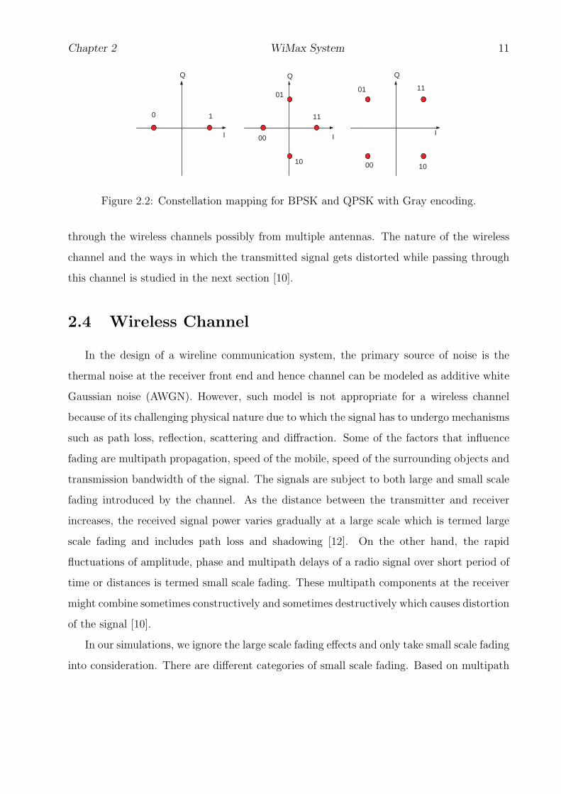
2.3.3 Constellation Mapping
The FEC code bits are mapped to the I and Q symbol co-ordinates using Gray code
mapping as shown in the Fig. 2.2 depending upon whether BPSK or QPSK is used. In Gray
encoding, the messages associated with signal amplitudes that are adjacent to each other
differ by one bit value. With this encoding, when the receiver makes a mistake in estimating
the transmitted symbol to its adjacent one (most likely), the result is only a single bit error
in the sequence of K bits [11].
The points in the constellation are symbols. For BPSK, they are√
Es and −√Es and for
QPSK, the four symbols can be found as {−√Es,√
Es,−j√
Es, j√
Es} or{√
Es
2+ j
√Es
2,√
Es
2− j
√Es
2,−
√Es
2+ j
√Es
2,−
√Es
2− j
√Es
2
}These modulated symbols are transmitted
Chapter 2 WiMax System 11
I I
Q Q Q
I
1 0
11 01
00 10
11
01
00
10
Figure 2.2: Constellation mapping for BPSK and QPSK with Gray encoding.
through the wireless channels possibly from multiple antennas. The nature of the wireless
channel and the ways in which the transmitted signal gets distorted while passing through
this channel is studied in the next section [10].
2.4 Wireless Channel
In the design of a wireline communication system, the primary source of noise is the
thermal noise at the receiver front end and hence channel can be modeled as additive white
Gaussian noise (AWGN). However, such model is not appropriate for a wireless channel
because of its challenging physical nature due to which the signal has to undergo mechanisms
such as path loss, reflection, scattering and diffraction. Some of the factors that influence
fading are multipath propagation, speed of the mobile, speed of the surrounding objects and
transmission bandwidth of the signal. The signals are subject to both large and small scale
fading introduced by the channel. As the distance between the transmitter and receiver
increases, the received signal power varies gradually at a large scale which is termed large
scale fading and includes path loss and shadowing [12]. On the other hand, the rapid
fluctuations of amplitude, phase and multipath delays of a radio signal over short period of
time or distances is termed small scale fading. These multipath components at the receiver
might combine sometimes constructively and sometimes destructively which causes distortion
of the signal [10].
In our simulations, we ignore the large scale fading effects and only take small scale fading
into consideration. There are different categories of small scale fading. Based on multipath

Chapter 2 WiMax System 12
time delay spread, the transmitted signal undergoes either flat fading or frequency selective
fading and based on Doppler spread the signal undergoes either fast or slow fading. The signal
undergoes flat fading when the bandwidth of the signal is less than the coherence bandwidth
of the channel or equivalently, if the symbol period is greater than the multipath spread.
Under these conditions, the received signal has amplitude fluctuations due to the variations
in the channel gain over time caused by multipath. However, the spectral characteristics of
the transmitted signal remain intact at the receiver. On the other hand the signal undergoes
frequency selective fading when the coherence bandwidth of the channel is much less than
the bandwidth of the transmitted signal or equivalently, if the symbol period is less than
the multipath spread. In this case, the received signal is distorted and dispersed, because
it consists of multiple versions of the transmitted signal, attenuated and delayed in time.
This leads to time dispersion of the transmitted symbols within the channel arising from
these different time delays resulting in intersymbol interference (ISI). A channel is classified
as slow fading if channel variations are much slower than the baseband signal variations or
equivalently, if the coherence time of the channel is much larger than the symbol period.
A signal undergoes fast fading if the symbol duration is larger than the coherence time of
channel.
2.4.1 Rayleigh Fading Distribution
The complex-baseband received signal in a multipath fading channel can be modeled as
rl(t) =L∑
n=1
αn(t)e−j2πfcτn(t)sl(t− τn(t)) (2.6)
Where L is the number of paths, {αn(t)}n and {τn(t)}n are the attenuation factor and
propagation delay respectively. These two fading parameters are modeled as random pro-
cesses as they keep varying and are not deterministic in nature. The delays are often con-
sidered to be uniformly distributed over a reasonable number of symbol periods. Rayleigh
fading distribution is a kind of probability distribution used to model the received signal
envelope, which is determined by {αn(t)}n. This model is used for channels that do not have
a strong LOS component. It assumes a large number of scatterers so that the central limit
Chapter 2 WiMax System 13
theorem leads to a Gaussian distribution for the fading coefficients. The fading coefficient
can be written as
α(t)e−j2πfcτ(t) = xa(t) + jya(t) (2.7)
where xa(t) and ya(t) are independent zero mean (because there is no strong line of
sight component) real Gaussian random processes. In such case,√
x2 + y2 has a Rayleigh
distribution and hence the received signal envelope, α(t) has a Rayleigh distribution with its
phase uniformly distributed over [0, 2π).
2.4.2 Block Fading
One of the simplest fading models for time varying channels is block fading [13]. Here, the
fading coefficients are modeled as constant over a block of symbols and vary independently
between blocks. The simulation becomes extremely simple because of the lack of correlation
among any fading coefficients. The received signal after lowpass filtering for a block consisting
of N symbols with duration T can be written as
rl(t) = hsl(t) + n(t), 0 < t ≤ NT (2.8)
where sl(t) is the baseband transmitted signal and h ∈ C is a random variable drawn
from a complex Gaussian distribution. Notice that h does not change during the block and
hence this model can be used for slow fading channels.
2.4.3 Performance of BPSK and QPSK
The analytical expression for the probability of bit error in AWGN channel for BPSK
or QPSK modulation is given by Q(√
2Eb
N0), with Eb
N0= γ being the signal-to-noise ratio.
The BER expression for a fading channel can be evaluated by averaging the error in AWGN
channel over the fading probability density function as
Pe =
∫ ∞
0
Pe(γ)p(γ)dγ (2.9)

Chapter 2 WiMax System 14
where Pe(γ) is the probability of error at a specific value of signal-to-noise ratio (SNR) γ
and p(γ) is the probability density function of γ of the fading channel. If we consider a unity
gain fading channel, p(γ) is simply the distribution of the instantaneous SNR in a fading
channel. Whereas for Rayleigh fading channels, the fading power |h|2 and hence the SNR γ
have an exponential distribution given as
p(γ) =1
γ0
exp
(− γ
γ0
)(2.10)
where γ0 = Eb
N0|h|2 is the average SNR. Therefore the average BER in a Rayleigh fading
channel can be calculated as
P =
∫ ∞
0
Q(√
2γ)1
γ0
exp
(− γ
γ0
)dγ (2.11)
The above equation can be evaluated to [14]
P =1
2
[1−
√γ0
1 + γ0
](2.12)
The BER equations exhibit an inverse algebraic relation between error rate and SNR for
a Rayleigh fading channel and an exponential relationship for an AWGN channel. The BER
curves for AWGN and Rayleigh fading channels are shown in Fig. 2.3. We can observe that
the BER performance in a Rayleigh fading channel is very poor compared to AWGN channel.
For example, an SNR of 24 dB is required to achieve a BER of 10−3 in the Rayleigh fading
channel which is achieved with 3 dB SNR in the AWGN channel. This poor performance can
be attributed to deep fades and in such environments the performance can be significantly
improved by diversity techniques and error control coding which we will study in the later
chapters.
2.5 Summary
WiMax primarily operates in two frequency bands: 10-66 GHz for LOS and below 11 GHz
for NLOS. The features of WirelessMAN-SCa PHY are described. The wireless channel is

Chapter 2 WiMax System 15
0 5 10 15 20 25 3010
−6
10−5
10−4
10−3
10−2
10−1
100
Eb/No (dB)
BE
R
BPSK in AWGNBPSK in Rayleigh fading
Figure 2.3: SNR vs BER for BPSK in AWGN and fading.
effected by small and large scale fading. Small scale fading can be flat or frequency selective
and slow or fast. The representation of signals in a flat and slow varying channel is described.
The wireless channel is modeled as a block Rayleigh fading channel. The phase-shift-keying
modulation scheme is studied and the signal degradation in a fading channel compared to
an AWGN channel is shown through simulation results.

16
Chapter 3
Multiple Antenna Systems
3.1 Introduction to Diversity
The two key issues in the physical layer level design of wireless communication are fad-
ing due to multipath propagation and interference of external signals. When a signal is
transmitted in a fading channel, the signals travel in multiple paths from the transmit-
ter to the receiver. These multiple versions of the transmitted signal, which will vary in
their amplitudes and phases as they go through different paths of the channel, can combine
either constructively or destructively at the receiver. The parameters like amplitude and
phase of these signals also varies very rapidly even with small movements of the transmit-
ter or receiver. Therefore fading leads to unreliable communication links. Interference can
be of several forms. Self interference is caused from reflected copies of the desired signal.
Co-channel interference is caused from other users of the same wireless network. External
interference is caused due to wireless signals originating outside the network. To build a
good wireless system we need to combat both fading and interference.
Diversity is a technique to combat fading and mitigation for interference. Diversity im-
proves the reliability of the wireless system by exploiting the multipath propagation property
of the radio channel. As in most of the wireless systems, the multiple copies of the received
signal are affected by independent fading phenomenon and the chances of reliable reception
is greatly increased at the receiver by making use of diversity techniques. The possible forms
of diversity are time diversity, frequency diversity, path diversity and antenna diversity. As

Chapter 3 Multiple Antenna Systems 17
the fading levels change with time, we can transmit the same signal at different times to
achieve time diversity. Forward error correction (FEC) coding and rake reception of spread-
spectrum signals may be considered as time diversity. A rake receiver anticipates multipath
propagation delays of the transmitted spread spectrum signal and combines the informa-
tion obtained from several resolvable multipath components to form a stronger version of
the signal [14]. Transmitting the signal at different frequencies forms frequency diversity,
spread-spectrum techniques and OFDM are forms of frequency diversity. Sending the sig-
nals over the wireless channel in many different paths forms path diversity. Transmitting or
receiving the signal through multiple antennas at slightly different locations forms antenna
diversity.
The original signal can be recovered by making use of the information of the desired
signal and the interference. The three widely used methods to mitigate interference are
designing a receiver which makes the optimum decision, the maximum a posteriori (MAP)
equalizers or maximum likelihood sequence equalizer (MLSE) which are very complex. The
second method to mitigate interference is to decorrelate the signal from the interference and
the third method is to estimate the interference and subtract it out. Same as diversity,
interference mitigation techniques can be performed in time, frequency or space [15].
3.1.1 Diversity Combining Techniques
Diversity combining of independently faded signals is a technique used at the receiver
to mitigate the effects of fading. Here the fact that the signal-to-noise ratio (SNR) of
the combined signals at the receiver is more than that of the individual branch SNR is
considered. Diversity techniques allow the receiver several chances to determine the correct
signal. As many replicas with a slight change in amplitude and/or phase of the original
signal are available at the receiver,the receiver has to process these signals in order to obtain
the desired signal. There three ways of processing or combining the signals are equal gain
combining, selection combining and maximal ratio combining [15].
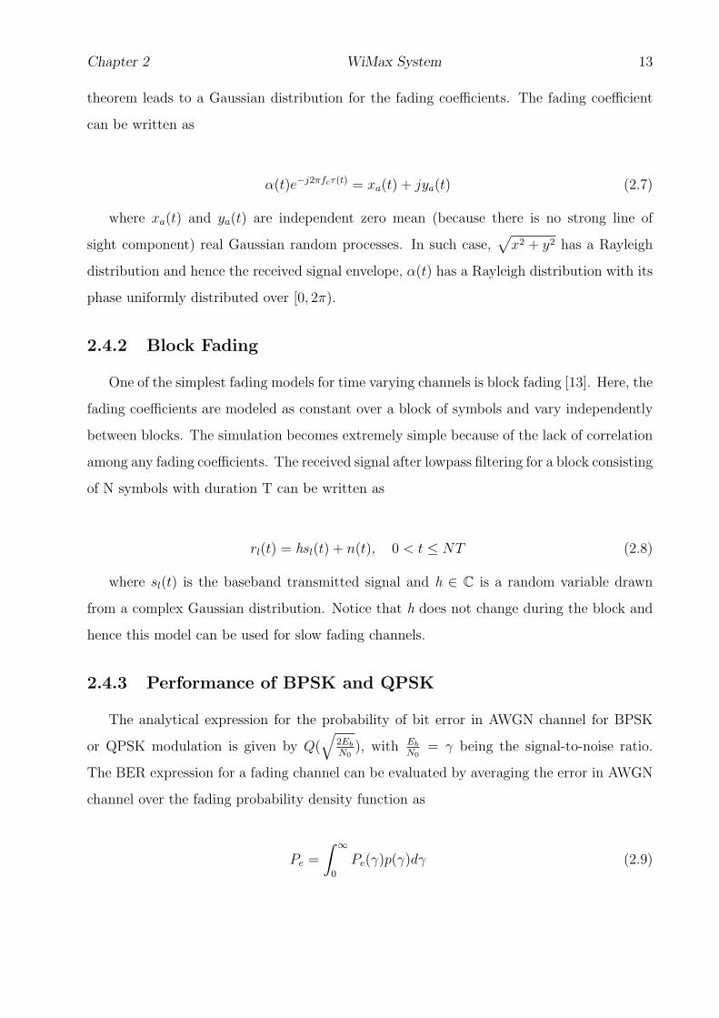
Fig. 3.1 shows diversity combining at the receiver. s(t) is the transmitted signal which
is received as r(t) at the receiver through various independent paths. α1 and α2 are the
Chapter 3 Multiple Antenna Systems 18
Transmitter
1 w
2 w
1 a
2 a 1 a
2 a
3 d
S(t)
S(t)
S(t)
r(t)
Figure 3.1: Diversity Combining at the Receiver.
fading coefficients of the two paths respectively. They can either be Rayleigh or Ricean
depending upon the presence of the line of sight. The distance between the antennas should
be a minimum of 3d, where d is the wavelength of the signal. The received signal r(t) can be
written as r(t) = w1α1s(t) + w2α2s(t) where w1 and w2 are the weights that are chosen by
the receiver to multiply with the signal on each of the diversity branch. Following diversity
combining techniques tell us how to choose the weight wl.
Maximal Ratio Combining
Maximal ratio combining (MRC) technique gives the best statistical reduction of fading
of any known linear diversity combiner and is the optimal one [14]. MRC improves on
other diversity schemes by coherently combining each diversity branch to provide the largest
possible SNR [10]. Assuming that there are L branches available, select weights w1, . . . , wl
to maximize the SNR of the combined decision statistic r =∑L
i=1 wlrl. we can interpret this
as weighting each decision statistic in direct proportion to the relative strength of the signal
component. We may use wl = |αl|, l = 1, ....., L. The instantaneous SNR of MRC can be
written as
γMRC =Es
∑Ll=1 |αl|
N0
(3.1)

Chapter 3 Multiple Antenna Systems 19
The average SNR for MRC is calculated as
γMRC = E[γMRC ] = γ.L (3.2)
where γ is the average SNR. MRC does not throw away any energy even from the low SNR
branches. Therefore, MRC coherently adds all available energy from all diversity branches,
yielding the largest possible average SNR. The analytical expression of the probability of
error for BPSK in the presence of L−branch diversity channel with MRC can be found by
averaging the BER of BPSK in AWGN, given by Q(√
2γ) over the distribution of SNR (γ)
of MRC. The analytical expressions for BER with BPSK and QPSK in Rayleigh fading can
be used to determine their performance [16]. For a L−branch channel they are calculated as
Pb,BPSK =1
2
[1− µ
L−1∑
l=0
(2l
l
)(1− µ2
4
)l]
,µ =
√γ0
1 + γ0
(3.3)
Pb,QPSK =1
2
[1− ρ
L−1∑
l=0
(2l
l
)(1− ρ2
4
)l]
,ρ =µ√
2− µ2(3.4)
γ0 =
Eb/N0, receive diversity
Eb/LN0, transmit diversity
In the Fig. 3.2, the lower curve indicates BPSK and higher curve QPSK. We can see that
the slopes of the curves are the same for both BPSK and QPSK for a particular branch. The
shift in the curve shows the coding gain where as the identical slope denotes that there is no
diversity improvement between BPSK and QPSK. Since MRC gives the optimal performance
by increasing the slope of the SNR-BER curve, it serves as a good reference for comparison
with any other diversity scheme. Therefore, a system whose BER curve has the same slope
as MRC but perhaps shifted to the right with L-branches is said to exploit full L-branch
diversity [10].
Selection Combining
The conventional selection combiner(CSC) selects the signal from that diversity branch
which has the largest instantaneous SNR, i.e. only the strongest decision statistic is used

Chapter 3 Multiple Antenna Systems 20
0 5 10 15 20 25 30 35 4010
−14
10−12
10−10
10−8
10−6
10−4
10−2
100
Eb/No (dB)
BE
R
L = 1
L = 2
L = 3
Figure 3.2: Bit error rate of BPSK (lower curve) and QPSK (higher curve) in a fadingchannel for L = 1, 2, 3 with MRC decoding
to compute the answer. The receiver simply decodes the branch with the largest SNR and
ignores the other branches.
wl =
1, if |αl| > |αj|,∀j 6= l
0, else(3.5)
Which means the instantaneous SNR of selection diversity can be written as
γSD =Esmaxl|αl|
N0
(3.6)
So that the average SNR can be written as where Es is the symbol energy and N0 is the
noise power of the signal.
γL = E[γSD] (3.7)
which evaluates to
γL = γ
(1 +
L∑
l=2
1
l
)(3.8)
where γ is the average SNR on each individual branch, and γL is the average SNR for L
branches. It can be clearly seen that γL>γ. It can also be seen that γSD < γMRC . According
Chapter 3 Multiple Antenna Systems 21
to a paper written by Ning Kong [17], he proposed a generalized selection scheme(GSC)
where instead of selecting only the largest instantaneous SNR diversity branch as in CSC,
m largest signals from L total diversity branches are selected and then coherently combined.
The average SNR of this GSC is found to be upper bounded by the average SNR of the
optimal diversity combining scheme MRC and lower bounded by the average SNR of CSC
scheme. The selection diversity scheme is not the best as the receiver throws away energy
from all other diversity branches other than the one with the largest SNR [17]. This is a
good choice when the signals fade independently where at least one signal will be strong and
usable.
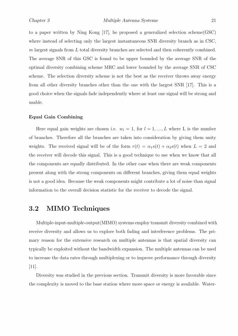
Equal Gain Combining
Here equal gain weights are chosen i.e. wl = 1, for l = 1, ...., L where L is the number
of branches. Therefore all the branches are taken into consideration by giving them unity
weights. The received signal will be of the form r(t) = α1s(t) + α2s(t) when L = 2 and
the receiver will decode this signal. This is a good technique to use when we know that all
the components are equally distributed. In the other case when there are weak components
present along with the strong components on different branches, giving them equal weights
is not a good idea. Because the weak components might contribute a lot of noise than signal
information to the overall decision statistic for the receiver to decode the signal.
3.2 MIMO Techniques
Multiple-input-multiple-output(MIMO) systems employ transmit diversity combined with
receive diversity and allows us to explore both fading and interference problems. The pri-
mary reason for the extensive research on multiple antennas is that spatial diversity can
typically be exploited without the bandwidth expansion. The multiple antennas can be used
to increase the data rates through multiplexing or to improve performance through diversity
[11].
Diversity was studied in the previous section. Transmit diversity is more favorable since
the complexity is moved to the base station where more space or energy is available. Water-

Chapter 3 Multiple Antenna Systems 22
filling [18] can be approached if feedback of the channel is available at the transmitter but
this can also be a disadvantage as the complexity increases. The other disadvantage with
transmit diversity is that it suffers a power penalty because the energy must be divided
between multiple antennas. Multiplexing exploits the structure of the channel gain matrix
to obtain independent signaling paths that can be used to send independent data [9]. Since
MIMO techniques improve the data rate and reliability of wireless communication by provid-
ing diversity advantage and coding gain through multiplexing, they are being employed on
almost all the PCS towers, WiFi base stations, WiMAX base stations. MIMO systems can
offer many times the throughput of conventional SISO wireless links without increasing the
transmitted power or bandwidth. The two categories of MIMO systems are space-time trel-
lis code (STTC) [19] and space-time block code (STBC) [8]. Both the schemes are types of
encoding procedures at the transmitter. The main goal of STBC is to obtain diversity advan-
tage where as that of STTC is both diversity advantage as well as coding gain which makes
the STTC system more complex than the STBC. Some hybrid schemes such as BLAST [20]
approach are also possible in which the emphasis is signal processing at the receiver. The
goal of these hybrid schemes is to achieve high data rates which makes them more complex.
They are discussed in detail in the further sections [15] .
The are several questions regarding space time codes that demand our attention. The
first question is whether space time coding can achieve the same diversity advantage as MRC.
The second question is can coding gain also be achieved in addition to diversity advantage
and how much bandwidth efficiency does these schemes provide [21]. The answers to these
questions are obtained by further detailed study.
3.2.1 Space-Time Block Codes
As a naive space time coding approach, we transmit the same data through the available
number of transmit antennas suppose for example two transmit antennas and one receive
antenna. After matched filtering, the received discrete-time signal at the single receive
antenna will be of the form
r =1√2(α0 + α1)s + n (3.9)

Chapter 3 Multiple Antenna Systems 23
Where s is the transmitted symbol, α0, α1 are the complex Gaussian channel coefficients
on the two paths between the receive antenna and transmit antennas 1 and 2, respectively,
and n is additive Gaussian noise. Since we are sending the same symbol from the two
transmit antennas, we have to divide the power among the two antennas, hence the square
root factor. At the receiver we multiply the received signal by (α1 + α2)∗, which yields the
decision statistic
y =1√2|α0 + α1|2b + v (3.10)
Where v is still a Gaussian noise sample. To determine the performance of this system, we
need to compare the pdf of the SNR to that of the 2-branch MRC. However, the distribution
of 1√2(α0 + α1) is same as the distribution of α0 or α1 alone. Therefore we get no diversity
gain by this method of sending the same data from the available number of antennas [10].
Orthogonal space-time block codes with nT transmit antennas and nR receive antennas
are coding strategies that provide full nT .nR diversity with little or no rate penalty. The
first example code of such kind is the Alamouti space time block code [8]. This two transmit
antenna code provides full 2.nR diversity with no rate penalty and very simple decoding.
Suppose we wish to transmit two symbols s0 and s1 over a flat fading channel with two
transmit antennas and one receive antennas (the example can be easily extended to more
receive antennas). Ideally, we would like to achieve a 2-branch MRC performance. We have
seen that transmitting each symbol separately from both antennas provides no transmit
antenna diversity gain. The Alamouti space time block code [8] matrix is
S =
[s0 s1
−s∗1 s∗0
](3.11)
where the row indicates the symbols transmitted from the two transmit antennas during
the first time slot, and the second row indicates the symbols transmitted during the second
time slot. The discrete-time received signal at antenna 1 during the two symbol intervals is
r0 = α0s0√2
+ α1s1√2
+ n0 (3.12)
r1 = −α0s∗1√2
+ α1s∗0√2
+ n1 (3.13)

Chapter 3 Multiple Antenna Systems 24
where the square root factor is needed to ensure unit transmit power for each symbol.
The noise samples n0 and n1 are independent and identically distributed complex Gaussian
zero-mean random variables with power N0. The estimates of the symbols at the receiver
are given by
s0 = α0∗r0 + α1r1
∗ =1√2(|α0|2 + |α1|2)s0 + α0
∗n0 + α1n1∗ (3.14)
s1 = α1∗r0 − α0r1
∗ =1√2(|α0|2 + |α1|2)s1 + α1
∗n0 − α0n1∗ (3.15)
The instantaneous SNR for each symbol is
|α0|2 + |α1|22N0
(3.16)
This system provides the same diversity performance as 2-branch MRC, although there
is a 3 dB SNR loss caused by the fact that we must split the transmit power across two
transmit antennas. Notice also that the Alamouti scheme transmits two symbols in two
time slots. Therefore the rate of the code is 1, which means there is no loss of bandwidth to
achieve full transmit antenna diversity. The Alamouti scheme [8] works because the columns
of the space-time block code matrix are orthogonal. A natural question to ask is, do space
time-block code matrices exist for more than two transmit antennas? The answer is yes,
but with qualifications. For complex symbols, there are no full-rate space-time block code
matrices for more than two transmit antennas. Tarokh [22] provided examples of lower rate
code matrices that provide full diversity.
Generalized Real Orthogonal Designs
A generalized real orthogonal design is a p×nT matrix G with entries 0,±x1,±x2, . . . ,±xk
such that GTG = (x12 +x2
2 + . . .+xk2)InT×nT
. p represents the delay required by the code.
The goal in the design of real STBC is to design a code that achieves full diversity nT nR for a
given number of transmit antennas nT and a given rate R = k/p. Because p represents delay
and lowers rate, the goal is to find designs which minimize p. Tarokh’s paper [22] provides
G for generalized real orthogonal designs for nT = 1, . . . , 8 and that have rate R = 1.
Generalized Complex Orthogonal Designs

Chapter 3 Multiple Antenna Systems 25
0 5 10 15 2010
−8
10−7
10−6
10−5
10−4
10−3
10−2
10−1
Eb/No (dB)
BE
R
STBC 2:1STBC 2:2STBC 2:3
Figure 3.3: Alamouti space time block code with QPSK in Rayleigh fading channel withMRC decoding.
A generalized complex orthogonal design is a p× nT matrix G with entries 0,±x1,±x2,
. . . ,±xk,±x1∗,±x2
∗, . . . ,±xk∗ such that G†G = (|x1|2 + |x2|2 + . . . + |xk|2)InT×nT
. Again
one goal of the code design is to minimize the required delay p to achieve full-diversity code.
Tarokh’s paper [22] presents designs G for rate 1/2 and rate 3/4 codes which achieve full
diversity. There do not appear to exist full-rate complex orthogonal design codes for more
than 2 antennas. For example if we have 3 transmit antennas and complex symbols, we can
use the matrix,
s0 s1 s2
−s1 s0 −s3
−s2 s3 s0
−s3 −s2 s1
s0∗ s1
∗ s2∗
−s1∗ s0
∗ −s3∗
−s2∗ s3
∗ s0∗
−s3∗ −s2
∗ s1∗
(3.17)
This scheme transmits 4 complex symbols over 3 antennas over 8 time slots. The columns

Chapter 3 Multiple Antenna Systems 26
are orthogonal, so full transmit antenna diversity with linear ML decoding, but the normal-
ized rate is 1/2, instead of 1, as in the Alamouti 2 transmit antenna scheme [8]. Similar rate
1/2 code matrices can be formed for four and more transmit antennas. Tarokh also provided
a few known special cases of higher rate codes (rate 3/4) for 3 and 4 transmit antennas.
If the modulation symbols are real, there exists full rate orthogonal space-time block code
matrices only for 2, 4, and 8 transmit antennas. For 4 transmit antennas, we can use
s0 s1 s2 s3
−s1 s0 −s3 s2
−s2 s3 s0 −s1
−s3 −s2 s1 s0
(3.18)
The design goals are to achieve full diversity nT nR where nT and nR are the number of
transmit and receive antennas respectively, to achieve full rate R = 1, to minimize delay p
and linear complexity at the receiver. For real constellations it is possible to achieve all these
goals upto 8 antennas where as for complex constellations it is not possible to achieve full
rate and full diversity for more than 2 antennas. It is possible to achieve rate 1/2 and 3/4
with full diversity for upto 4 antennas for complex constellations. Note that higher spectral
efficiencies can be obtained even without full rate, by using larger signal constellations [15].
Note that there is no memory between consecutive blocks and that the typical block
length is very short and thus a very limited coding gain is expected. The scheme has a
very simple decoding structure and therefore it can be concatenated to a powerful outer
error correction code. STBCs are limited in the number of transmit antennas that can be
supported and still obtain an orthogonal design. At the decoupling stage, the combiner
assumes that each received signal is composed by a linear superposition of current symbols
corrupted by noise. This is not the case in high delay spread environment where there exists
a strong channel-induced ISI component. Thus, the performance of STBC might be sensitive
to such environments. Nevertheless, the scheme is still an appealing one for its simplicity
and can be examined in conjunction with known techniques for e.g rake receiver [15].

Chapter 3 Multiple Antenna Systems 27
3.2.2 Space-Time Trellis Coding
Space-time trellis codes (STTCs), are an extension of the conventional trellis codes to
MIMO systems [19]. The criteria that have been primarily applied to the design of STTCs are
the rank and determinant. They are described by a trellis diagram where this STTC maps k
input bits and v state bits into nT simultaneously transmitted symbols by using nT generator
polynomials. The decoding consists of channel estimation using ML sequence estimation via
the Viterbi algorithm. The advantage of a well constructed STTC is that it achieves both
diversity advantage and coding gain. The diversity advantage is the asymptotic slope of the
error rate curves while coding gain is the offset in SNR from an uncoded system with same
diversity advantage. Therefore, this STTC is a robust technique for a variety of mobility
environments [19]. The major drawbacks are the complexity of the decoder increases expo-
nentially with bandwidth efficiency in a STTC whereas STBC extracts excellent diversity
gain which has much remarkably low decoder complexity. However, though STBCs achieve
full diversity advantage, as they do not provide coding gain, their performance is inferior to
that of STTCs which achieve both full diversity gain as well as coding gain. Added coding
gain to STTCs as well as STBCs can be achieved by concatenating these codes either in
serial or in parallel with an outer channel code. One more drawback is that there is a lack
of general STTC constructions [19] [15].
3.2.3 BLAST Techniques
BLAST stands for Bell Labs layered space time architecture and was proposed by Foschini
et al. from Bell labs [20]. It uses multiple transmit and receive antennas to obtain diversity
by exploiting the rich scattering environment [9]. The transmitter transmits different sub
channels through different antennas without including any orthogonality. The receiver uses
sorting and multiuser detection technique to obtain the sub channels. The detailed procedure
is studied in the coming sections. The channel assumptions for BLAST systems are that,
the channel is known before hand and has a large number of multipath. The bandwidth
is considered to be narrow well within the flat fading zone of the channel. A Quasi-static
channel is assumed where the channel does not change significantly with in the symbol

Chapter 3 Multiple Antenna Systems 28
duration. There are two types of BLAST techniques D-BLAST and V-BLAST.
D-BLAST
D-BLAST is a diagonal layered space time architecture in which coding is introduced
between streams across diagonals in space-time. Here the data stream is first parallel encoded
and rather than transmitting the codeword with one antenna, the codeword symbols are
rotated across antennas, so that a codeword is transmitted by all the nT transmit antennas
present. As a result the codeword is spread across all spatial dimensions [15].
Vector Encoder
V-BLAST Signal Processing
RX
RX
RX
RX
TX
TX
TX
TX data
RX data
Rich scattering Environment
Figure 3.4: V-BLAST
V-BLAST
V-BLAST is considered to be the encoding of serial data into a vertical vector and hence
referred to as vertical encoding. Thus, each antenna acts as a conventional transmitter with
a single stream of data. It can achieve at most a diversity order of nR, since each coded
symbol is transmitted from one antenna and received by nR antennas [20]. There are a
number of schemes for the detection of V-BLAST that are relatively easy to implement and
provide high performance.
• Original Algorithm (Zero Forcing, No-Ordering)
• Modified Algorithm (Zero Forcing, Optimal detection order)
• Maximum Likelihood Algorithm

Chapter 3 Multiple Antenna Systems 29
Consider the number of transmit antennas to be nT and receive antennas nR. The
transmitted data is represented in the form of a vector as x = [x1x2x3 . . . xnT]T whose
dimensions are (nT ×1). The received vector will be of the form r = Hx+v with dimensions
(nR×1) where v is a complex Gaussian noise vector with zero mean and variance σ2(nR×1)
[15]. Channel matrix H with dimensions (nR × nT ) is given as
H =
h(1,1) . . . h(nT ,1)
......
h(1,nR) . . . h(nT ,nR)
(3.19)
The only difference between the original algorithm and modified algorithm is the selection
of the first symbol to be decoded. In the modified decoding algorithm, first the strongest
signal is decoded. Then, canceling the effects of this strongest symbol from all the received
signals by considering the interference from all other symbols as noise, the algorithm detects
the next strongest symbol. This way the algorithm continues by canceling the effects of the
detected symbol and the decoding of the next strongest symbol until all the symbols are
detected. This original algorithm works only when the number of receive antennas is more
than that of the transmit antennas, that is nR > nT [23]. The algorithm includes three steps
◦ ordering
◦ interference cancelation
◦ interference nulling
The purpose of ordering step is to decide which transmitted symbol to detect at each
stage of the decoding. The symbol with highest SNR is the best pick in this step. The
goal of interference cancelation is to remove the interference from the already detected sym-
bols in decoding the next symbol. Finally, interference nulling finds the best estimate of
a symbol from the updated equations. This step is called interference nulling since it can
be considered as removing the interference effects of undetected symbols from the one that
is being decoded. Zero-forcing(ZF) and Minimum mean-square error(MMSE) are the two
types of nulling techniques. MMSE gives a better performance than ZF. Maximum likelihood
algorithm makes a decision by considering only the closest neighbors in the constellation [23].
The main goal of BLAST systems is to substantially increase the throughput by using
multiple antennas. This approach assumes that the number of receive antennas is greater

Chapter 3 Multiple Antenna Systems 30
0 2 4 6 8 10 12 1410
−4
10−3
10−2
10−1
Eb/No (dB)
BE
R
V−BLAST 2:2V−BLAST 2:3
Figure 3.5: V-BLAST for QPSK using ML detector
than or equal to the number of transmit antennas. No orthogonality between the spatially
separated signals is required at the transmitter and the channel should have rich scattering
environment [15] .
3.3 Summary
In this chapter, the methods to combat fading are explained by introducing the concept
of diversity. Spatial diversity is taken as the point of interest and hence various diversity
combining techniques used at the receiver end, to combine the multipath signals are studied
and compared. It is concluded that MRC gives the optimal performance and hence any sys-
tem with spatial diversity can be compared with MRC to evaluate its performance. Further,
MIMO systems where spatial diversity is included both at the transmitter as well as the
receiver are introduced. The two primary MIMO systems, STBCs and BLAST systems are
studied in detail and their performances for different antenna configurations is plotted.

31
Chapter 4
Turbo Coding for WiMax
4.1 Channel Coding for WiMax-IEEE 802.16-2004
The WirelessMAN-SCa PHY supports several combinations of modulation and coding
rates that can be used to achieve various trade-offs of data rate and robustness, depending
on channel and interference conditions for both uplink and downlink. One of the FEC codes
it supports is a concatenated FEC which uses an outer Reed-Solomon code (RS) [24] and an
inner convolutional code [25] with optional interleaving between the outer and inner codes.
The second FEC option is turbo coding which can be achieved either by a block turbo
code (BTC) or a convolutional turbo code (CTC). Turbo coding can improve the coverage
and/or capacity of the system, at the price of increased decoding latency and complexity
[26]. Although the BTC and CTC are optional in the initial WiMax standards, they are
made mandatory in the next and latest versions. There is also a no-FEC option supported
by the standard where an automatic repeat request (ARQ) mechanism is used to transmit
data reliably instead of FEC coding. In this project, we implement a convolutional turbo
code as the FEC and further study the details of a turbo code in this chapter [5].
4.2 The need for Channel Coding
In 1948, Shannon demonstrated in a landmark paper [27] that, by proper encoding of the
information, errors induced by a noisy channel can be reduced to any desired level without

Chapter 4 Convolutional Turbo Code 32
sacrificing the rate of information transmission, as long as the information rate is less than
the capacity of the channel. Therefore, coding for error control in a noisy environment is
being used in almost all high speed communication systems [28]. Applying FEC coding in a
wireless channel reduces the probability of bit error due to its error correction capability.
The amount of error reduction provided by a given code is typically characterized by
its coding gain in AWGN and diversity gain in fading. Since FEC provides time diversity
by adding redundancy to the data, we use it in addition to the multiple antennas which
provides spatial diversity. Therefore, a channel code concatenated with MIMO, and with
an appropriate modulation scheme, is proven to provide very good performance in a fading
channel [11].
In Fig. 2.1, we see in the transmitter block that the modulator follows the channel
encoder. The function of this channel encoder is to introduce, in a controlled manner,
some redundancy in the binary information sequence, which can be used at the receiver to
overcome the effects of noise and interference encountered in the transmission of the signal
through the channel. The encoding process generally involves taking a k-bit sequence into
a unique n-bit sequence, called a code word [16]. The amount of redundancy introduced by
the encoding of the data in this manner is measured by the ratio n/k. The reciprocal of the
ratio, k/n is called code rate [28].
At the receiver, the demodulator processes the signals which are impaired by the channel
and reduces each signal to a scalar or vector that represents an estimate of the transmitted
data symbol. The detector, which follows the demodulator, may decide on whether the
transmitted bit is a 0 or a 1 (M=2). The detector quantizes the demodulator’s metric to
one of the quantization (Q) levels. The demodulator is said to make hard decisions when it
has output quantization (Q=2 for M=2) in which case the decoder will have binary inputs.
When the output of the demodulator is quantized to more than two levels, i.e. Q > 2 (or the
output is left unquantized), the demodulator is said to make soft decisions. In this case, the
decoder must accept multilevel or continuous valued inputs which makes its implementation
difficult. Hard decisions in the demodulator result in some irreversible information loss as
it discards information that can reduce probability of codeword error [29]. For example, in
BPSK (M=2), the received symbol is decoded as 1 if it is closer to√
Eb and 0 if it closer to
Chapter 4 Convolutional Turbo Code 33
−√Eb. Here, the distance of the received symbol from√
Eb and −√Eb is not being used in
decoding, yet this information can be used to make better decisions about the transmitted
codeword. In soft decision decoding, the demodulator makes a soft decision corresponding
to the distance between the received symbol and the symbol corresponding to a 0-bit or a
1-bit transmission [11]. In this chapter, the structure of the CTC which supports various
frame sizes and code rates and the calculation of the soft values (LLRs) which are given as
inputs to the decoder are studied.
4.3 Convolutional Turbo Coder
4.3.1 Introduction
Convolutional turbo codes [30], also called parallel concatenated convolutional codes
(PCCC) were first introduced in 1993 by Berrou et al.. Today almost all the advanced FEC
systems employing turbo codes are capable of achieving moderately low BERs of around
10−5 at SNRs within 1 dB of the Shannon limit [27] [28]. Turbo codes are proven to provide
higher throughputs and higher data rates within the given power constraints.
4.3.2 CTC Encoder
The CTC encoder as depicted in the Fig. 4.1 has three main blocks, the constituent
encoder, the interleaver and the puncturer. It uses a double binary circular recursive sys-
tematic convolutional code (CRSC) [31]. The term double binary implies that the encoder
can accept two data bits per time instance and thus gives out four bits totally including the
two systematic bits and the two parity bits. The CRSC encoding is performed in such a
way that it should make sure that the initial and final states of the encoder are the same,
which makes it circular. The CTC encoder can take in several frame sizes of information
bits ranging from 32 bytes to 1024 bytes either in the form of E bits or F couples. As seen in
Fig. 4.1, the polynomials defining the encoder connections are given as 1 + D + D3 for the
feed back branch and 1+D2 +D3 for the Y parity bit. The information bits are fed through
inputs A and B alternately starting with the most significant bit (MSB) of the first byte. In

Chapter 4 Convolutional Turbo Code 34
the first step, A and B are directly taken as outputs also called systematic bits without any
encoding and then they are fed into the constituent encoder 1 whose structure is shown in
the figure. It gives out the parity bits Y1 and W1. In the second step, the same information
bit sequences A and B are passed through the interleaver and then the interleaved informa-
tion bits are fed to the constituent encoder 2 which is similar to constituent encoder 1. This
produces the parity bits Y2 and W2. The final codeword can be formed as ABY1W1Y2W2.
Since there are four parity bits and two systematic (data) bits, the code rate is 1/3. Further
code rates can be obtained by puncturing the code words [32] [5].
A
B
CTC Interleaver Constituent Encoder Puncturer
Y 1 Y 2
W 1 W 2
A
B
Switch
D D D
W Y
A
B
CTC Block Diagram
Constituent Encoder
Figure 4.1: CTC encoder with a Constituent encoder.
The important aspect of the constituent encoder is attaining the circulation state Sc,
where the initial and final states of the encoder are equal. In recursive encoding, this state
is obtained by performing the following steps. First, encode the information sequence after
initializing the encoder to all zeroes state and determine the final state in case of natural
order and in case of interleaved order. In both the cases, this ending state is represented as
SN which is further used to calculate the circulation state Sc by some linear algebra methods

Chapter 4 Convolutional Turbo Code 35
based on the state space description of the encoder. But alternately, the IEEE 802.16-2004
standard provides a circulation state look-up table shown in Fig. 4.2 to determine Sc based
on SN and the frame size N. Now after initializing the encoder to Sc determined from the
look-up table, the information sequences are encoded again to obtain the parity bits. This
time the encoder is guaranteed to end in state Sc as it is set to initially [33] [5]. Considering
Sk as the state at time k which is represented by a 3 element column vector (8 possible
states) containing the values stored in the D-flip flops in the Fig. 4.1, the encoder state at
time k can be related to the state at time k-1 as
Sk+1 = GSk + Xk (4.1)
and
Y = [ 1 1 0 ]Sk+1 + [Ak + Bk] (4.2)
where
Xk =
Ak + Bk
Bk
Bk
(4.3)
and
G =
1 0 1
1 0 0
0 1 0
(4.4)
4.3.3 CTC Interleaver
Interleaving the data along with coding increases the performance of the system. With
a linear code, it is desirable to produce high weight codewords (e.g. codewords with a large
number of 1’s) because it is the lowest nonzero weight codeword that sets the minimum
distance of the code and, hence, the error correcting capability of the code. Suppose that
a particular message causes a low weight output from the constituent encoder 1, when the

Chapter 4 Convolutional Turbo Code 36
0 1 2 3 4 5 6 7
1
2
3
4
5
6
S N
N mod 7
0
0
0
0
0
0
6
3
5
4
2
7
4
7
3
1
5
6
2
4
6
5
7
1
7
5
2
6
1
3
1
6
7
2
3
4
3
2
1
7
4
5
5
1
4
3
6
2
Figure 4.2: Circulation State Look up Table for IEEE 802.16-2004.
same message is interleaved and sent through the constituent encoder 2, it is not likely to
also produce a low weight output. Thus, in a turbo code it is unlikely that both encoders
simultaneously produce low weight outputs, and hence, the number of low weight codewords
is very small, leading to the good performance of turbo codes. Before passing the information
sequences A and B through the second encoder, the data is interleaved at two levels as follows
Step 1 : For every even value of j, i.e. if (jmod2 == 0) Interchange Aj and Bj, i.e. make
(Aj, Bj) = (Bj, Aj) where j = 1, 2, .....N . This is interleaving between the couples.
Step 2 : This step involves interleaving within the couples. Here we need a parameter
P0 which shall be the nearest prime number greater than√
N/2. We compute the function
Pj(i) which gives the interleaved address i of the considered couple j. First, we calculate
(jmod4) which can be 0, 2, 3 or 4. If 0 or 2, we get i = (P0.j + 1)modNand if it is 3 or 4 we
get i = (P0.j + 1 + N/4)modNfor j = 1, 2, .....N . The bits at the address positions j and i
will be switched. These interleaved bits are fed to the second encoder [5] [33].
4.3.4 CTC Puncturer
The CTC puncturer selectively deletes parity bits in order to provide various code rates.
The puncturing patters to be followed are specified in the standard. To obtain code rates
1/2 and higher, all the W parity bits are deleted. For rate 1/2, all the Y parity bits are
transmitted, for rate 2/3, every even indexed bit of Y is transmitted and for rates 3/4, 5/6,

Chapter 4 Convolutional Turbo Code 37
and 7/8 every fourth, sixth and eighth bits are transmitted respectively [5] [33].
The order in which these encoded bits are given to the BPSK or QPSK symbol mapper is
A0, B0, ...., AN−1, BN−1, Y10, Y11, ...., Y1M , Y20, Y21, ...., Y2M where, N is the information frame
size and M is the Y parity bits block size for both interleaved and uninterleaved data. These
bits are mapped according to the signal constellations shown in the third chapter [5].
4.4 CTC Decoder
The practical importance of turbo and serial concatenated codes lies in the availability
of a simple suboptimum decoding algorithm [30]. Turbo decoding relies on the exchange
of probabilistic information between the two soft-input soft-output (SISO) decoders [34].
Usually, and also in our implementation, the probabilistic information is expressed in the
form of log likelihood ratio (LLR). The role of a SISO decoder consists of taking input LLR
estimates of the transmitted bits and trying to improve these estimates by using the local
redundancy of the considered component code [34]. The iterative decoders such as max-log-
MAP [35] and log-MAP used in this project are based on maximum a posteriori probability
(MAP) algorithm [34]. The detailed procedure to implement the CTC decoder can be seen
in [33]. In this project implementation, the software used to simulate the CTC coded system
leverages code developed at the Wireless Communications Research Laboratory (WCRL)
and made available under the GPL license within the Iterative Solutions Coded Modulation
Library (ISCML)1. In the next section, the soft inputs or the LLRs to be given as inputs to
the decoder are derived.
4.4.1 Calculation of the input LLRs to the decoder
The bitwise log likelihood ratios of the systematic bits and the parity bits are to be
calculated at the output of the demodulation stage and given as inputs to the CTC decoder.
In the implementation discussed here, we consider QPSK modulation, a 2 × 1 Alamouti
space time block code [8], i.e. two transmitters and one receiver, Rayleigh fading channel
1Iterative Solutions Coded Modulation Library, available at http://www.iterativesolutions.com/Matlab.htm,release 1.6.2 edition, July 2006

Chapter 4 Convolutional Turbo Code 38
and MRC diversity combining at the receiver. The procedure to followed to calculate the
bit LLRs is shown below.
The discrete signal model for a slow varying, flat fading channel can be written as
R = HS + N (4.5)
where R is the received symbol vector, S is the transmitted symbol vector, N ∼ Nc(0, σ2I)
is the AWGN vector, and H the channel gain matrix given by
H =
[h11 h21
h∗21 −h∗11
](4.6)
where h11 and h21 are the complex channel gains between the two transmit antennas and
one receive antenna. The decision statistic ’d’ at the receiver for MRC decoding is given by
d = HHR (4.7)
In a two transmit one receiver case,
s =1√2
[s1
s2
](4.8)
d =
[d1
d2
](4.9)
d1 and d2 are calculated to be
d1 =1√2Ehs1 + n1 (4.10)
d2 =1√2Ehs2 + n2 (4.11)
where Eh = |h11|2 + |h21|2, n1 and n2 are the complex Gaussian noise with mean 0 and
variance σ2. From equations of d we can see that, σ2d = Ehσ
2. As described in the previous
chapter, for QPSK modulation, we suppose 00 −→ 1, 01 −→ j, 11 −→ −1, 10 −→ −j. From
Chapter 4 Convolutional Turbo Code 39
this, we can describe the symbol sets S(0)1 = {1, j} is the set of symbols whose first bit is a
0, S(1)1 = {−1,−j} is the set of symbols whose first bit is a 1, S
(0)2 = {1,−j} is the set of
symbols whose second bit is a 0, S(1)2 = {−1, j} is the set of symbols whose second bit is a
1. The LLR for the k’th bit of the i’th symbol can be calculated as
λk(di) = ln
(Σ
s∈S(1)k
P (si|di)
Σs∈S
(0)k
P (si|di)
)(4.12)
where i = 1, 2 for each estimated symbol. The equation of the LLR for the first bit of
the first symbol d1
λ1(d1) = ln
(P (s1 = −1|d1) + P (s1 = −j|d1)
P (s1 = 1|d1) + P (s1 = j|d1)
)(4.13)
= ln
(f(d1|s1 = −1) + f(d1|s1 = −j)
f(d1|s1 = 1) + f(d1|s1 = j)
)(4.14)
If λ1(d1) > 0, the first bit of d1 = 1 or if λ1(d1) < 0, the first bit of d1 = 0.
Similarly, the LLR for the second bit is given by
λ2(d1) = ln
(f(d1|s1 = −1) + f(d1|s1 = j)
f(d1|s1 = 1) + f(d1|s1 = −j)
)(4.15)
If λ2(d1) > 0, the second bit of d1 = 1 or if λ2(d1) < 0, the second bit of d1 = 0. By
replacing d1 with d2 in the equation 4.15, we can find the bit LLRs for d2.
The conditional probability density functions (pdfs) in the equation 4.15 need to be
calculated to get the value of LLRs. From the equations of d1 and d2, we can see that d1
depends only on s1 and not on s2. Hence d1 is the decision statistic for s1. Similarly d2 is
the decision statistic for s2. Consider the case when the first symbol s1 = 1, we can write
d1 = d1,r + jd1,i where d1,r = 1√2Eh + n1,r is the real part and d1,i = n1,i is the imaginary
part with variance σ2d = Ehσ
2.
d1,r is a Gaussian random variable with mean ’ 1√2Eh’ and variance ’σ2
d’. Therefore its pdf
can be written as
fd1,r(d1,r|s1 = 1) =1√
2πσd
exp
−
(d1,r − 1√
2Eh
)2
2σ2d
(4.16)

Chapter 4 Convolutional Turbo Code 40
d1,i is a Gaussian random variable with mean ’0’ and variance ’σ2d’. So its pdf will be
fd1,i(d1,i|s1 = 1) =
1√2πσd
exp
[− (d1,i)
2
2σ2d
](4.17)
The Conditional pdf of d1 given s1 = 1 is given as
fd1(d1|s1 = 1) = fd1,r(d1,r|s1 = 1).fd1,i(d1,i|s1 = 1) (4.18)
=
(1
2πEhσ2
)exp
−
∣∣∣d1 − 1√2Eh
∣∣∣2
2σ2Eh
(4.19)
Similarly the conditional pdfs f(d1|s1 = −1), f(d1|s1 = j), f(d1|s1 = −j) are calculated
and substituted in the equation to find out the bit LLRs. These LLRs for the whole codeword
at the output stage of the demodulator are calculated and given as inputs to the decoder.
4.5 Summary
One of the channel coding options provided in IEEE 802.16-2004 standard is the convo-
lutional turbo coding. It outperforms the other channel coding options such as concatenated
FEC and also is less complex than block turbo coding. The CTC encoder, interleaver and
puncturer are described in detail and the procedure involved to calculate the CTC decoder
input LLRs is described.

41
Chapter 5
Results and Conclusions
5.1 Performance of Concatenated STBC and CTC for
WiMax
The Performance of a wireless system is significantly improved by the application of both
multiple-input-multiple-output (MIMO) techniques and convolutional turbo codes (CTC).
As we have seen in the previous chapters, MIMO techniques provide spatial diversity gain
by combating the fading effects of the multipath channel and turbo codes provide significant
coding gain. However, just using the space time block code (STBC), a type of MIMO
technique without an outer channel code is not enough. Even soft decoding of STBC will not
significantly improve the performance due to the lack of new extrinsic information [36]. Also,
in slow fading channels, just turbo coding together with interleaving without MIMO cannot
be that effective as delay and latency considerations limit the depth of interleaving. Deep
fades can cause severe error propagation in the iterative decoding process [37]. Consequently
it is desirable to concatenate the STBC with the CTC to simultaneously achieve the large
diversity gains provided by the STBC and error correction capability of the CTC.
5.1.1 System Model for BWA Applications
The Rayleigh fading channel for broadband wireless access (BWA) systems exhibits slow
fading as well as flat fading with no significant line-of-sight (LOS) component. Therefore,

Chapter 5 Results and Conclusions 42
channel response is constant over the entire length of a turbo codeword, and varies inde-
pendently from frame to frame. A single-carrier system is considered for the simulations.
Additive white Gaussian noise (AWGN) is added at the receiver for every received symbol.
The randomly generated binary data couples of a particular frame size F are first turbo en-
coded by passing it through the CTC which constitutes of a double binary circular recursive
systematic convolutional code (CRSC) with rate 1/3. Alternate higher code rates are possi-
ble by puncturing the output obtained for rate 1/3 as explained in Chapter 4. In our results
we show and compare the bit-error-rate curves for code rates 1/3, 1/2, 3/4. These turbo
encoded bits which constitute the parity bits as well as the systematic bits are modulated by
the QPSK (M = 4) symbol mapper as studied in Chapter 2. This mapper maps groups of
two bits into one of four complex symbols from a unit power Gray coded QPSK constellation.
Next, these QPSK symbols are transmitted by using two antennas (nT = 2). We make use
of the Alamouti space time block code (2Tx:1Rx) with two transmitters and one receiver to
introduce transmit diversity as studied in Chapter 3. After space time coding, if OFDM were
to be used, the resulting channel symbols would be transmitted through several sub-carriers
which provides frequency diversity. However, we use a single carrier in our simulation to
transmit the modulated symbols over the multipath fading wireless channel.
The signal gets distorted by the slowly fading channel as well as AWGN. The channel
coefficients generated randomly for every turbo codeword, are uncorrelated circularly sym-
metric complex Gaussian with mean zero and unity variance. The noise random variables
generated for every symbol, are uncorrelated circularly symmetric complex Gaussian with
mean zero and variance σ2 which varies with the average signal-to-noise-ratio (SNR). At
the receiver, we assume the channel state information to be known and perform maximal
ratio receiver combining (MRRC) to obtain the decision statistic vector d as described in
the STBC section in Chapter 3. At each time instance, the d vector will have dimensions
2× 1, i.e. two symbols for the considered Alamouti STBC (2:1). These symbols have to be
further processed in order to obtain the soft bits or the log likelihood ratios (LLRs) which
are exploited by the turbo decoder. Calculation of these LLRs for STBC (2:1) with QPSK
modulation is described in the last section of Chapter 4. For orthogonal STBCs, such as the
Alamouti code, the complexity for computing these LLRs increases only linearly with the

Chapter 5 Results and Conclusions 43
number of transmit antennas. On the contrary, due to the lack of orthogonality, the com-
plexity in calculating the LLRs rises exponentially with the number of transmit antennas
when V-BLAST is used [38]. Finally, these soft bits are given as inputs to the CTC decoder
to obtain the turbo decoded outputs. The turbo decoder uses the max-log-MAP algorithm
[35].
5.2 Results
The performance results of the considered IEEE 802.16-2004 standard are shown in Fig.
5.1. These curves are obtained for frame size, F = 24 bytes and 16 iterations. We can see
that there is a performance increase as the code rate decreases. In Fig. 5.3, the uncoded and
coded STBC with nT = 2, nR = 1 for code rate 1/3 are compared. We can see that there is
a 4 dB difference between the curves which is attributed to the coding gain provided by the
CTC. These curves are also compared with a single-input-single-output (SISO) turbo coded
system in Fig. 5.4, where we can see that there is a diversity gain between the turbo coded
SISO and STBC. In Fig. 5.2 throughput curves of the IEEE 802.16-2004 system for different
code rates are shown. The throughput T is calculated by the equation T = R(1− FER), R
being the code rate and FER being the frame error rate.
5.3 Conclusions
Fixed broadband wireless access is an ideal solution for providing high data rate com-
munications where conventional systems like DSL and cable modems are either unavailable
or too costly. It can be concluded that the performance of BWA systems can significantly
be improved by space time block codes by providing diversity gain. Further improvement is
achieved by concatenating the STBC with an outer channel code like a turbo code.
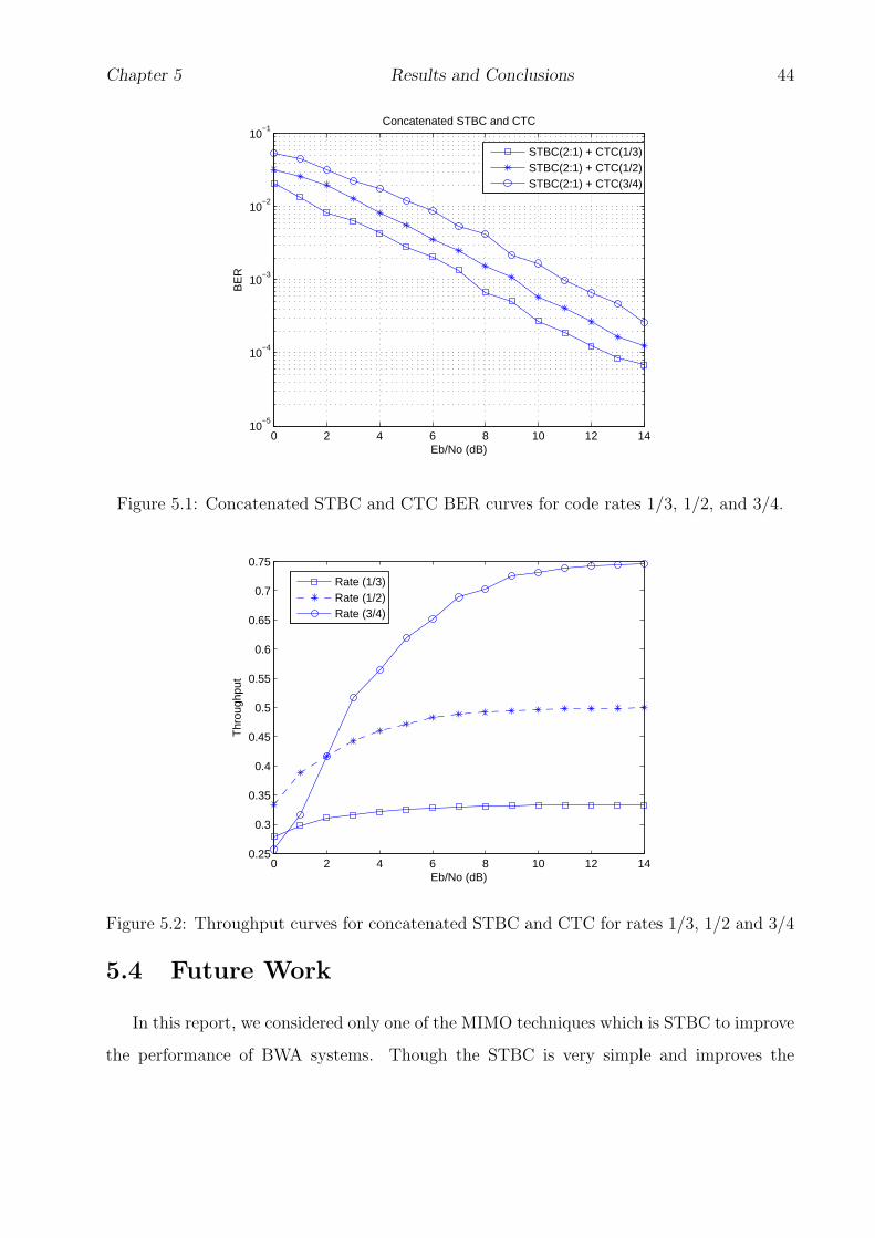
Chapter 5 Results and Conclusions 44
0 2 4 6 8 10 12 1410
−5
10−4
10−3
10−2
10−1
Eb/No (dB)
BE
R
Concatenated STBC and CTC
STBC(2:1) + CTC(1/3)STBC(2:1) + CTC(1/2)STBC(2:1) + CTC(3/4)
Figure 5.1: Concatenated STBC and CTC BER curves for code rates 1/3, 1/2, and 3/4.
0 2 4 6 8 10 12 140.25
0.3
0.35
0.4
0.45
0.5
0.55
0.6
0.65
0.7
0.75
Eb/No (dB)
Thr
ough
put
Rate (1/3)Rate (1/2)Rate (3/4)
Figure 5.2: Throughput curves for concatenated STBC and CTC for rates 1/3, 1/2 and 3/4
5.4 Future Work
In this report, we considered only one of the MIMO techniques which is STBC to improve
the performance of BWA systems. Though the STBC is very simple and improves the

Chapter 5 Results and Conclusions 45
0 5 10 15 2010
−5
10−4
10−3
10−2
10−1
Eb/No (dB)
BE
R
Comparison of coded and uncoded STBC (2:1)
STBC (2:1)STBC (2:1) + CTC (1/3)
Figure 5.3: Comparison of coded and uncoded STBC for rate 1/3
0 5 10 15 20 25 3010
−4
10−3
10−2
10−1
100
Eb/No (dB)
BE
R
SISO + CTC(1/3)uncoded STBC(2:1) STBC(2:1) + CTC(1/3)
Figure 5.4: Comparison of SISO-CTC, uncoded STBC and coded STBC
reliability of the system, the data rates achieved are not as high as with V-BLAST. Also, we
considered only a single carrier system because of which there is no frequency diversity. By
Chapter 5 Results and Conclusions 46
using OFDM, frequency diversity is exploited. Therefore a STBC-CTC or a V-BLAST-CTC
with OFDM will give better performance. The concatenation of STBC with a block turbo
code (BTC) might also be simple and lead to a performance improvement. Furthermore,
since the row (or column) encoding (or decoding) of the BTC coding can be implemented in
parallel, the computation efficiency can be further improved.

47
References
[1] J. E. Gaskin, Broadband Bible, Wiley, 2004.
[2] A. A. Gilroy and L. G. Kruger, “Broadband internet access: Background and issues,”CRS Issue Brief for Congress, Dec. 2003.
[3] D.J. Johnston and M. LaBrecque, “IEEE 802.16 wirelessman specification accelerateswireless broadband access,” Technology@Intel Magazine, Aug. 2003.
[4] H. Blcskei, A. J. Paulraj, K. V. S. Hari, and R. U. Nabar, “Fixed broadband wirelessaccess:State of the art, challenges, and future directions,” IEEE Commun. Magazine,vol. 39, pp. 100–108, January 2001.
[5] IEEE Computer Society, and IEEE Microwave Theory and Techniques , IEEE 802.16-2004 standard for Local and metropolitan area networks. Part 16 : Air Interface forFixed Broadband Wireless Access Systems, October 2004.
[6] A. Zakhia, Y. Peng, and Chang, J.M, “WiMax: The emergence of wireless broadband,”IT Professional, vol. 8, pp. 44–48, Jul-Aug 2006.
[7] S. Nadkarni K. Seshadrinathan R. Simha l. J. Doyle, K. Han and I. C. Wong, “Per-formance evaluation of the IEEE 802.16a physical layer using simulation,” EE381K-11(14980)Wireless communication project report.
[8] S. Alamouti, “A simple transmit diversity technique for wireless communications,”IEEE J. Select. Areas Commun., vol. 16, no. 8, pp. 1451–1458, Oct. 1998.
[9] G. Foschini, and M. Gans, “On the limits of wireless communications in a fadingenvironment when using multiple antennas,” Wireless Personal Commun., vol. 6, no.3, pp. 311–335, 1998.
[10] D. Reynolds, “Wireless communication systems,” Course Notes, WVU, Fall 2003.
[11] A. Goldsmith, Wireless Communication, Cambridge University Press, 1995.
[12] G. S. Prabhu and P. Mohana Shankar, “Simulation of flat fading using matlab forclassroom instruction,” Department of Electrical and Computer Engineering, DrexelUniversity.
REFERENCES 48
[13] R. Knopp, and P. A. Humblet, “On coding for block fading channels,” IEEE Trans.Inform. Theory, vol. 46, pp. 189–205, January 2000.
[14] T. Rappaport, Wireless Communication Systems, 3rd ed., New York, NY: McGraw-Hill,1995.
[15] B. Woerner, “Multi antenna systems,” Course Notes, WVU, Spring 2005.
[16] J.G. Proakis, Digital Communications, 3rd ed., New York, NY: McGraw-Hill, 1995.
[17] N. Kong, “Performance of generalized selection diversity combining for both iid andnoniid Rayleigh fading channels,” Proc. IEEE Military Commun. Conf. (MILCOM),pp. 1584–1589, 2004.
[18] R. G. Gallager, Information Theory and Reliable Communication, Wiley, New York,NY, 1968.
[19] V. Tarokh, N. Seshadri, and A. R. Calderbank, “Space-time codes for high data ratewireless communications: Performance criterion and code construction,” IEEE Trans.Inform. Theory, vol. 44, no. 2, pp. 744–765, Mar. 1998.
[20] G. Foschini, “Layered space-time architecture for wireless communication in a fadingenvironment when using multi-element antennas,” Bell Labs. Tech. Journal, vol. 1, no.2, pp. 41–59, Autumn 1996.
[21] L. Zheng, and D. Tse, “Diversity and multiplexing: A fundamental tradeoff in multipleantenna channels,” IEEE Trans. Inform. Theory, vol. 49, pp. 1073–1096, May 2003.
[22] V. Tarokh, H. Jafarkhami, and A. R. Calderbank, “Space-time block codes from or-thogonal designs,” IEEE Trans. Inform. Theory, vol. 45, no. 5, pp. 1456–1467, July1999.
[23] H. Jafarkhani, Space-Time Coding, Cambridge University Press, 2005.
[24] I. S. Reed, and G. Solomon, “Polynomial codes over certain finite fields,” Journal ofApplied Mathematics (SIAM), vol. 8, pp. 300–304, 1960.
[25] P. Elias, “Coding for noisy channels,” IRE Conv. Rec., vol. 3, pp. 37–46, March 1955.
[26] A. Ghosh, D. R. Wolter, J. G. Andrews, and R. Chen, “Broadband wireless access withWiMax/IEEE 802.16:Current performance benchmarks and future potential,” IEEECommun. Magazine, vol. 35, no. 9, 2005.
[27] C. E. Shannon, “A mathematical theory of communication,” Bell Labs. Tech. Journal,pp. 379–423 (Part 1); 623–56 (Part 2), July 1948.
[28] S. Lin, and D. J.Costello, Error Control Coding, Prentice Hall, 2004.
[29] B. Vucetic, and J. Yuan, Turbo Codes, Kluwer Academic Publishers, 2000.

REFERENCES 49
[30] C. Berrou, A. Glavieux, and P. Thitimajshima, “Near Shannon limit error-correctingcoding and decoding,” Proc. IEEE Int. Conf. on Commun. (ICC), Geneva, Switzerland,vol. 2, pp. 1064 – 1070, May. 1993.
[31] C. Berrou, C. Douillard, and M. Jezequel, “Multiple parallel concatenation of circularrecursive convolutional (CRSC) codes,” Annals of Telecommunication, pp. 166–172,Mar.-Apr. 1999.
[32] G. Richter B. Baumgartner, M. Reinhardt and M. Bossert, “Performance of forwarderror correction for IEEE 802.16e,” University of Ulm, and Siemens AG, October 2006.
[33] M.C. Valenti, S. Cheng, and R. Iyer Seshadri, “Turbo and LDPC codes for digitalvideo broadcasting” Chapter 12 of Turbo code applications: A journey from a paper torealization, Springer, 2005.
[34] C. Berrou, R. Pyndiah, P. Adde, C. Douillad, and R. Le Bidan, “An overview of turbocodes and their applications,” Wireless Technology. The European Conference on, pp.1–9, October 2005.
[35] P. Robertson, P. Hoeher, and E. Villebrun, “Optimal and sub-optimal maximum aposteriori algorithms suitable for turbo decoding,” European Trans. on Telecommun.,vol. 44, no. 2, pp. 8(2):119–125, Mar./Apr. 1997.
[36] G. Bauch, “Concatenation of space-time block codes and turbo-TCM,” Proc. IEEEInt. Conf. on Commun. (ICC), Geneva, Switzerland, vol. 2, pp. 1202–1206, June 1999.
[37] H. El Gamal and A. R. Hammons, Jr., “Analyzing the turbo decoder using the Gaussianapproximation,” IEEE Trans. Inform. Theory, vol. 47, pp. 671–686, Feb. 2001.
[38] I. J. Wassell I. A. Chatzigeorgiou, M. R. D. Rodrigues and R. A. Carrasco, “Turbocoded OFDM / SC-FDE techniques for MIMO BFWA channels,” Technichal report,Laboratory for Communication Engineering, University of Cambridge; Network Com-munications and Mobile Computing Research Group, University of Wolverhampton,Jan. 2005.