simulation of sulfate-dependent sulfate reduction using monod kinetics

Mathematical Geology, Vol. 19, No. 3, 1987

Simulation of Sulfate-Dependent Sulfate Reduction Using Monod Kinetics 1

L e o n a r d R o b e r t G a r d n e r 2' 3 a n d I a n L e r c h e 2

A simple computer code is presented for simulating the dependence of sulfate reduction on sulfate concentration using Monod kinetics. Unlike previous models, the code provides a numerical initial value problem solution, rather than a two-point boundary value solution, for the Monod model using a search procedure to find the correct starting value for the derivative of sulfate concentration with respect to depth. Accordingly the code is not restricted to cases where sulfate vanishes at finite depth but also can be used to model situations where organic matter is exhausted before total depletion of sulfate can occur. In such situations, the code demonstrates that profiles generated using Monod kinetics differ significantly from those generated using the simple sulfate-independent model proposed by Berner (1964), even when the asymptotic concentration of sulfate at depth remains well above the Monod saturation constant.

KEY WORDS: sulfate reduction, Monod kinetics, anoxic sediments, simulation model.

INTRODUCTION

In a recent paper, Boudreau and Westrieh (1984) discussed the dependence of bacterial sulfate reduction on sulfate concentration in marine sediments. Cor- roborating earlier studies (Martens and Berner, 1977; Ramm and Bella, 1974; Hallberg et al., 1976; Bagander, 1977; and Jorgensen, 1983), they present experimental results which show that the rate of sulfate reduction decreases dra- matically as the concentration of sulfate drops below about 5.0 millimolar (raM). They also show that the dependence of the rate of sulfate reduction on sulfate concentration can be described accurately by the "Monod" equation (Monod, 1949)

R = RmS/ (S + Ks) (1)

where R is rate of sulfate reduction (in mM yr-1), S is concentration of sulfate

~Manuscript received 1 August 1986; accepted 3 October 1986. 2Department of Geology, University of South Carolina, Columbia, South Carolina. 3Belle W. Baruch Institute for Marine Biology and Coastal Research, University of South Carolina, Columbia, South Carolina 29208.

219

0882 8121/87/0400 0219505.00/I © 1987 International Association for MathematicaI Geology

220 Gardner and Lerche

(in mM), R m is maximum rate and Ks is concentration at which R equals Rm/2. This is not to say, however, that the Monod equation provides an accurate description of the actual chemical mechanism of sulfate reduction. Indeed, mechanisms that control kinetics of sulfate reduction are poorly understood, and possibly some other equation eventually will be formulated that will not only describe experimental results but will be rooted in kinetic theory. How- ever, the Monod equation appears to be the best description available at present.

Unfortunately, incorporation of Monod kinetics into differential equations that describe the steady-state diagenesis of organic matter and sulfate leads to nonlinear ordinary differential equations that are not amenable to analytic solution. Accordingly, Boudreau and Westrich (1984) endeavored to evaluate several approaches for formulating sulfate-dependent diagenetic models. These in- eluded (1) modification of the original Berner (1964) model, (2) numerical solution of the Monod model, and (3) linearization of the Monod model. As the modified Berner model and the linearized sulfate-dependent models produced profiles sufficiently similar to the "theoretically preferred but less tract- able Monod model," Boudreau and Westrich advised the use of the former because it involves fewer unknown parameters and is easier to use. The purpose of this paper is to present a simple numerical procedure for the theoretically preferred Monod model. Unlike most of the procedures proposed by Boudreau and Westrich, our procedure does not require that the sediment contain enough organic matter to completely exhaust the available sulfate at a finite depth. Our procedure can explore the effect of Monod kinetics of sulfate profiles in sediments with subcritical amounts of organic matter. It also can be used to evaluate the zeroth-order appoximate solution for the Monod model suggested (but not tested) by Boudreau and Westrich (1984, p. 2515) for obtaining solutions in cases where organic matter is subcritical and the rate of sedimentation is slow compared to rates of decomposition and diffusion (i.e., "large oz" as discussed below).

SULFATE-DEPENDENT DIAGENETIC MODELS

The original Berner (1964) model assumes that the rate of decay of organic matter via sulfate reduction can be described by simple first-order kinetics

dG / dt = - k G (2)

where G is the concentration of particulate organic matter in the sediment and k is an appropriate rate constant in units of reciprocal time. Accordingly, at steady state, decomposition of organic matter is compensated by the divergence of the burial flux of organic matter.

w(dO/d ) = - k o ( 3 )

Simulation of Suifate-Dependent Sulfate Reduction Using Monod Kinetics 221

where w is transport velocity, x is depth, and the total derivative d / d t is then identical to w ( d / d x ) because O/c3t is zero at steady state.

Similarly, the consumption of interstitial sulfate is supported by divergence of its diffusive and burial fluxes

d2S dS D~-~5 - w-~, - f kG : 0 (4)

where S is sulfate concentration, Ds is the diffusion coefficient of SO4, w is burial velocity and

f - L(1 - 4~)P, (5) 4

where q~ is porosity, p, is mean density of solids, and L is the stoichiometric coefficient that relates consumption of sulfate to decay of organic matter. Hence f converts concentrations from a basis related to total sediment volume to one dealing with pore volume available for water.

In nondimensional form, Eqs. (3) and (4) can be written as

dT - - o ~ T ( 6 )

dz

d20 ldO - - - = r where (7)

dz 2 c~dz

= ( k ~ t/2 z x (8 )

T : I G / S ( o ) (9)

o = s / s ( o ) ( lo )

el =- ( D , k ) ' / Z / w (11)

As boundary conditions for Eqs. (6) and (7), Berner (1964), specified

T = T ( o ) at z = 0 ( 1 2 )

0 = 1 at z = 0 ( 1 3 )

dO/dz -o 0 as z --+ oo (14)

Accordingly, the solution for the original Berner model is

r ( o ) [1 - exp ( - c~z ) ] (15) 0 = 1 (c~ 2 + 1)

Thus, 0 will be positive at all depths only if T(o) < (c~ 2 + 1). In cases where


T(o) > (c~ 2 + 1), 0 becomes negative at finite depth. In order to deal with this situation, Boudreau and Westrich (1984, p. 2515) modified boundary conditions for Eqs. (6) and (7) such that at the critical depth z¢ where sulfate vanishes

0 = 0 (16)

dO/dz = 0 (17)

According to these authors, the analytic solution for the modified Berner model is

°t2T( O ) I (c~2 + 1)] [1 _ exp ( z / a ) ] 0 = 1 (c~ 2 + 1 )exp - zc ~

T(o) (c~ 2 + 1) [1 - exp ( - ~ z ) ] (18)

The value of Zc can be derived from the implicit expression obtained by substi- tution of 0 = 0 and z = Zc is Eq. (18). Although the modified Berner model does not explicitly describe any dependence of sulfate reduction on sulfate concentration, it gives results that nearly coincide with those obtained by Boudreau and Westrich for the Monod model. However, it cannot be applied to the case where T(o) < (c~ 2 + 1) for which one might wish to ascertain whether the original Berner model and the Monod model coincide.

The nondimensional equations for the Monod model are

d20 1 dO

dT

dz

TO

dz 2 ot dz K + O

olTo

K + O (19)

Because Boudreau and Westrich were interested in the case where sulfate is exhausted before organic matter, they specified the following boundary conditions

0 = 1 at z = 0 (21)

0 ~ 0 as z--} c~ (22)

T = T(o) ~ z = 0 (23)

With these boundary conditions, Eqs. (19) and (20) constitute a standard two- point boundary value problem on a semiinfinite domain. By trial and error se- lection of a sufficiently large but finite depth, numerical solutions were obtained using the finite-difference code PASVA3 (Lentini and Pereyra, 1977). Boudreau and Westrich (1984) were able also to transform the Monod model into a linear two-layer model by specifying that, above critical depth zo where 0 = K, Eqs.

- - - 0 ( 2 0 )


(6) and (7) govern whereas below Zo Eqs. (19) and (20) govern. At z = Zo, the additional boundary conditions are

0 = K (24)

0 + = 0 - ( 2 5 )

dO dO _ (26) Y z + =

T + = T - (27)

The analytic solution to the linearized Monod model yields profiles of 0 that coincide almost exactly with those produced by the modified Bemer model (Boudreau and Westrich, 1984, Fig. 2). However, at depths where 0 - K, the finite-difference numerical solution to Eqs. (19) and (20) gives somewhat larger values of 0 than those given by the modified Berner and linearized Monod models. More important is the fact that the value of 0 will be slightly positive but analytically unspecifiable if T(o) is slightly less than the critical value required for sulfate exhaustion and z = ~ . In such a case, Eqs. (19) and (20) cannot be treated as a two-point boundary value problem but must be ap- proached as an initial-value problem.

In order to deal with cases where T(o) is less than that required for complete sulfate exhaustion [i.e., subcritical T(o)], Boudreau and Westrich (1984) suggested a zeroth-order approximate solution for Eqs. (19) and (20). Their approximate solution approaches the true solution as c~ approaches infinity (i.e., large c~), in which case Eq. (20) reduces to

d20 TO - 0 ( 2 8 )

dz 2 g -t- O

Multiplication of Eq. (28) by c~ followed by addition to Eq. (19) and integration yields

o~(dO/dz ) = T ( m ) - T (29)

By obtaining a first integral of Eq. 28, Boudreau and Westrich were able to reduce the order of Eq. (28) so that the differential equation for sulfate becomes first-order as follows

dz - c~ Kln + 0(c~) + 0(co) - 0 (30)

The value of 0(c~) can be found by combining Eqs. (29) and (30) and applying the result at z --- 0. This yields the following implicit relationship between T(o) /e~ 2 and 0(~)


T(o) I K + 1 l (31) c~ 2 - 1 - 0 ( ~ ) - K l n K + 0 ( ~ )

Because 0(~) can be obtained implicitly from Eq. (31) for given values of T(o) and c~, Eq. 30 can be solved numerically (via Runge-Kutta) as an initial value problem. For further details on their derivation the reader is referred to Bou- dreau and Westrich (1984, p. 2515).

T H E MONOD I N I T I A L VALUE CODE

In order to numerically solve Eqs. (19) and (20) as an initial value problem using Runge-Kutta (or some other initial value procedure), values of 0 = T at z = 0 must be specified as well as the value of dO/dz. Unfortunately, no analytic procedure for specifying dO/dz at z = 0 is known, so one must resort to a trial and error procedure. However, constraints can be employed to guide such a procedure. A mathematical analysis of these constraints is presented in Ap- pendix A for the interested reader and can be sketched briefly as follows. For any physically realistic solution, 0 must lie between 0 and 1 at all z. The greater limit of 0 is imposed by the fact that Eqs. (19) and (20) do not contain source terms for the production of sulfate at depth. Accordingly, the initial value of dO/dz cannot exceed zero and, in fact, must be at least slightly negative because the Monod kinetic term (TO/(K + 0)) in Eq. 20 imparts positive curvature at z = 0. Furthermore, because sulfate is not produced at depth, dO/dz can never become positive. Inspection of Fig. 2 in Boudreau and Westrich (1984) reveals that the initial slope of 0 profiles generated by the original Berner model are always more negative than slopes of other models. Thus, the initial slope of the original Berner model, which can be specified analytically, can be used as the lesser limit of dO/dz at z = 0. As a first guess then, one can average the greater and lesser limits on the initial value of dO/dz and proceed to integrate using Runge-Kutta continuing until either (1) 0 becomes negative, (2) dO/dz becomes positive, or (3) a preselected, sufficiently large, terminal value of z is reached. If integration terminates because of condition 1, redefine the lesser limit for the initial value of dO/dz as the previous guess and average the new lesser limit and the current greater limit to provide a new guess for dO/dz at z = 0. Simi- larly, if integration terminates because of condition 2, redefine the greater limit for the initial value of dO/dz as the previous guess and average the new greater limit and the current lesser limit to obtain a new guess for dO/dz at z = 0. With repeated application of this procedure, limits on the initial value of dO/dz rap- idly narrow and, after about 55 iterations, the 16-digit (double) precision of a typical main frame computer will be exhausted. By this point, one will have determined accurately the shape of the 0 curve in at least the upper part of the simulated sediment. In cases where T(o) is greater than that required for total consumption of sulfate using the original Berner model, the last several itera-


tions preceding exhaustion of double precision will produce profiles that typ- ically are indistinguishable down to the depth where 0 drops below 0.001. Thus, for all practical purposes, an acceptable solution has been obtained even though condition 1 or 2 may be violated at greater depth because of insufficient precision and/or round-off error. In cases were T(o) is less than that required for total consumption of sulfate, condition 3 may be reached before exhaustion of precision if the terminal value of z is not sufficiently large. Here, one could simply increase the terminal value of z and rerun the calculations, but this can become prohibitive in computer time and volume of output. Alternatively, an additional criterion can be inspected upon reaching condition 3. In the case of subcritical T(o), 0 will not reach zero but as z approaches infinity both slope and curvature of 0 will approach zero. Thus if upon reaching condition 3 the curvature (i.e., d20/dz 2) is negative, the initial value of dO/dz is too negative because integration beyond terminal z will eventually result in violation of condition 1. One then can redefine the lesser limit for the initial value of dO/dz and try another iteration. On the other hand, if upon reaching condition 3 the slope is negative, but the curvature is still positive, one has no alternative other than to increase the terminal value of z and rerun the calculations. This rarely happens if the terminal value of z is greater than 10.

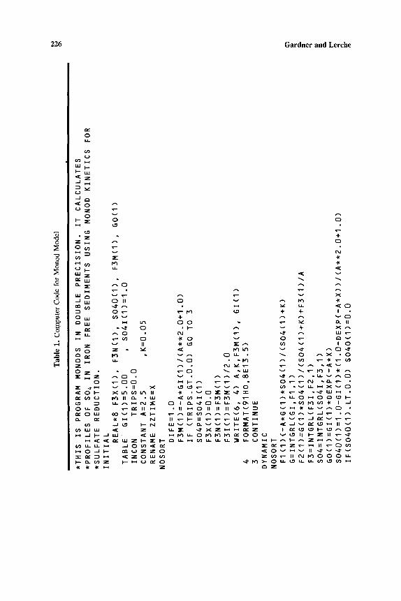
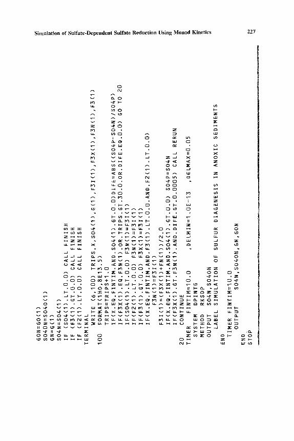
A simple code (MONODS) to perform these trial and error calculations is presented (Table 1). In order to avoid the labor of writing subroutines for integration and graphical output, we have used the IBM Continuous Systems Mo- delling Program III (Speckhart and Green, 1976).

CODE RESULTS

In order to compare MONODS with results obtained by Boudreau and Westrich (1984) using the finite-difference code PASVA3 (Lentini and Pereyra, 1977), we ran MONODS with the same parameter values shown in their Fig. 2 (i.e., T(o) = 10; K = 0.05; c~ = 0.1, 0.2, 0.5, 1.0, 2.0, 2.5, 3.0). In addition, we ran MONODS with a = 5.0 to show its behavior when T(o) is subcritical.

Results of these calculations (Fig. l) agree exactly with results obtained by Boudreau and Westrich (1984) using PASVA3. On the other hand, for subcritical T(o) (i.e., e~ = 5.0 for T(o) = 10), MONODS does not coincide exactly with the original Bemer model (i.e., Eq. 15). At large z, asymptotic values of 0 are 0.592 and 0.615, respectively, or about a 4% disagreement even though both are an order of magnitude greater than K ( - 0 . 6 versus 0.05). In cases where T(o) is only slightly below its critical value (e.g., c~ = 3.1 for T(o) = 10), relative disagreement is much greater. For example, with T(o) = 10, a = 3. t , and K = 0.05, MONODS gives an asymptotic 0 of about 10 -7 whereas the original Berner model gives 0.057. At the critical value itself (i.e., c~ = 3.0 for T(o) = 10), 0 approaches zero at infinity for both models although the


0

" 0 0

0

o

o

M

[..,

0

w

~ v u - J t-~

~ 0 ~ ~ z ..~ ~ - ~ o

• Z

0 ¢ n , r - ~-i .m~ V

U') X

IL l ; [

~ : ILl I~. Z , ' ~ 0

O W ¢ . ~ v +

Z u . ~ 0 t~J

Z v II ¢ 0

0 . • - 0 ~ r - O

0 ~"- 0 0

' ~ 0 b X u'~ o"~ t,"~ II

0 u _ ,--~ ~ 0 ~ ~0

r.~ - J

0 ~E n~

c

v Z , " ~

0 u -

"~. ~ L L I

~ v v ~ O

~ O l & ~ O ~ - ~ ~ 1 1 ~ , l l ~ O I I I I I l { V 3

N I I ~ I I ~ r ~ ~ N ~ v v ~ v v v W Z ~ Z ~ Z ~ X Z ~ Z

- ~ ~ O ~ O O U

¥ 0

v

÷ + I

~ 1 1

0 ~ ~ v m I 0

~ 0 ~ X , O

~ v ~ X ~

~ 0 ~ 0 ~

v ~ v ~ 0 •

~ v ~ v ~ ~ v ~ l l v

~ Z ~ 0

~ I I ~ O 0 0 ~ J ~ ~ O Z Z O ~ 0 V H ~ ~ Z O ~


0

v O- 0 ~ I - -

u - 0 0'~ cO 0 ~ -

~ 0 • Z ~

X ~ UJ ~-- ~ II X ~-~ t,~. ,--I Z - J X 0

O0 • O0 _.1

u . - o • O C ) u'~

~ C~ Z f~3 bO

,~- CD • • C3 1 Z

m • • ~ ~ ' - ~'-" 0 • • <E

~l" ~-~ n~ II U_ U- • C ) ,.-~ r'~ ~ ~ 0 0 ~'- ~ - - ~ II II --~ . ~ m . =iE : :3 LO

X 0 0 Z ~-" ~-~ I~1 ~ 0 ' ~ ~ : 3

~"'~ IJ TM , Z ~." , "~ Z ~ " Z Z ~." 0 ~ " O~: • <E Z (~ ~-. ,.-. ~E v u. ~( Z 0 F-IV) C) ./,r~ .EDED . ~--~ + .i~ Z ;E O~

• :[: u- O . :E I~ ,-~ :E u- E3 O 0 0 -

ED OO + I-- (~ I-- • I-- II v I-- I-- ED Oi-- ED ",~"

C 3 - O ~ Z L U . - I I - - I - - Z * - ~ X Z ¢ ~ O ~ - ~ D O 0 ~ ~ " 0

~O ~-- O{: • ~-- ~'- --~ ~'~ • Z ~-~ • x-- LU ~ ~-~ OO ,~I" :E

I ~ II I)J X - d ' v v U-I L L ~ LU X Z Z r ~ ~ bO O~

~--- 2E m'~ X ~ ~ u_ u_ X v X u.. i-- LL -J LL. "--~ ~.~ ~," m~ v v v v v v m--4 v v Z IE r~ ~--- mmm ~.

~z: ~ I.-- I - . - ~ ~ " 0 LU >'- I.U ~ ~-~ ~ - o"> ~ 0 . ' ~ - -

CD ~ z ~J I - - uJ

~ . - 4 Z Z

._J

. . d ~ J . ~ , ~ . J . . J

<.> ~J

. O C J

. C ~ C )

o ¢.~, - J

• " - ' 0 " 4 " v ~ ' - ' ~ -

~0 Z v II 0'~ U.. u.. Z i# 0 (.5 Z u v v ~-~ Z - . d " II ",,t" ~ " O O Z O U - ~ - ~ 0

. o . 0

z D-- I.~ oo

228 G a r d n e r a n d L e r c h e

DIMENSIONLESS CONCENTRATION

0 0 .5 1 0

( ,O0.5. ¢0 o~

~0.5" .J z 0 0 - -

~ - _ 0 0

1.5- 1

0


0 .5

I - ' ' "

os!f t, , , o , - - l o

1 0

w w _~ : O~ : 0 . 5

O 1" ] 0 1


0 0 . 5 1 i i o rD

~o. No.5 Z 0

~_ ot = 2 . 0

Q 13


0 . 5 1

f , T(O) = 10

O/ = 3 . 0

0 . 5 0

.I- I " n UJ r, u) 0.5- a)

z 0

IE

1.5,

i o-

mm 0.5.

z

R 1.5-


0 . 5 1 , J

T(0 ) - -10

OL --0.2


0 . 5 1

T (0 )= 10

(3( =1 .0


0 .5 1

T (O)=10

Ol = 2 .5


0 . 7 5 1

1 /

~1 ot --5.o

Fig. 1. Model profiles of the dimensionless sulfate concentration (Eq. 10) versus d imensionless depth (Eq. 8) for various values of parameter c~ (Eq. 11) with a d imensionless init ial organic matter concentra- t ion T(o) of 10 (Eq. 9) and a saturation constant K of 0.05. Dashed

line is the original Bemer model (Eq. 15), solid l ine is Monod model using PASVA3 as g iven by Boudreau and Westr ich (1984), and solid

circles are discrete values generated by MONODS (Table 1).


approach is somewhat more rapid for the Berner model. However, whereas T approaches zero in the Berner model, it stabilizes at an asymptotic value of about 0.33 in the Monod model. This is because the initial value of dO/dz is slightly more positive in the Monod model than in the Berner model; corre- spondingly, the diffusive flux of sulfate into the sediment is slightly less. This, in turn, prevents complete consumption of the initial organic matter. In general, when T(o) is greater than or equal to its critical value, values of 0 predicted by the Berner model, at least, are slightly less than those predicted by the Monod model at all depths. When T(o) is less than its critical value, values of 0 predicted by the Berner model again are slightly less, at least, than those predicted by the Monod model, but only at shallow depths. At greater depths, Monod values for 0 eventually drop below those for the Berner model. Again, this is due to the smaller diffusive flux of sulfate into the sediment for the Monod model. Although the smaller diffusive flux of sulfate in the Monod model in- hibits decomposition of organic matter, it ultimately permits greater depletion of sulfate when T(o) is subscritical.

DISCUSSION

Boudreau and Westrich (1984) reported that they were unable to extract parameter values (i.e., T(o), or, K, Zc) from actual data by nonlinear regression of either the modified Berner model or sulfate-dependent models on real data. They attribute this failure to scatter in, and sparsity of, actual data, especially for the zone of small sulfate concentration. As an alternative, they were able to demonstrate the magnitude of errors involved in estimating T(o) and e~ using the original Berner model rather than a sulfate-dependent model. This was done by using the linearized sulfate-dependent model to generate synthetic data sets, and then regressing the original Berner model on this data. Disagreements between assumed and extracted values of both T(o) and o~ were often as large as a factor of 2 or greater, indicating that errors in using the original Berner model are not negligible. Nonetheless, in an earlier section of their paper, they state (p. 2506) that, in cases where organic matter is exhausted before sulfate vanishes, the original Berner model is completely valid. In order to ascertain the correctness of this statement, we used MONODS to generate synthetic data sets for cases where T(o) is subcritical. Results show (Table 2) that in most cases values of T(o) and e~ extracted using the original Berner model are about 10% smaller than corresponding values of T(o) and c~ used in the Monod model to generate the synthetic data. Although these errors are not nearly as dramatic as those generated by Boudreau and Westrich for supercritical conditions, they nonetheless are significant. This is particularly so for ~ because the rate constant k is a function of c~ 2. Thus a 10% error in c~ will generate approximately a 20% error in k. The relative disagreement between Monod and Berner parameter values does not diminish noticeably with departure of T(o) from its critical


Table 2. Parameters Used to Generate Synthetic Data Using Monod Model and Those Extracted from Synthetic

Data Using Original Berner Model (K = 0.05)

Monod Bemer T(o) ot T(o) ot

10.0 3.0 10.0 3.0 3.1 8.61 2.78 3.5 8.67 3.10 4.0 13.52 4.66 5.0 9.36 4.69 7.0 8.87 6.38

5.0 2.0 4.80 1.98 2.1 4.49 1.93 2.5 4.54 2.27 3.5 4.25 3.08 5.0 7.91 6.40 7.0 4.43 6.39

value (i.e., as c~ increases). Thus, even though the asymptotic value of 0 at depth may be an order of magnitude greater than the saturation constant K, the original Berner model is still capable of introducing significant error in T(o) and t~ as compared to the Monod model.

As to whether MONODS could be used to extract values of T(o), a , and K from actual data using nonlinear regression, obviously the code is too complex to be used as a model in SAS or BMDP. In principle, one should be able to write a nonlinear regression code that would incorporate MONODS as a model. Undoubtedly, the code would be complex and is beyond the scope of this paper. In any event, as noted by Boudreau and Westrich (1984), successful parameter extraction undoubtedly will depend upon density and quality of sulfate concentration measurements.

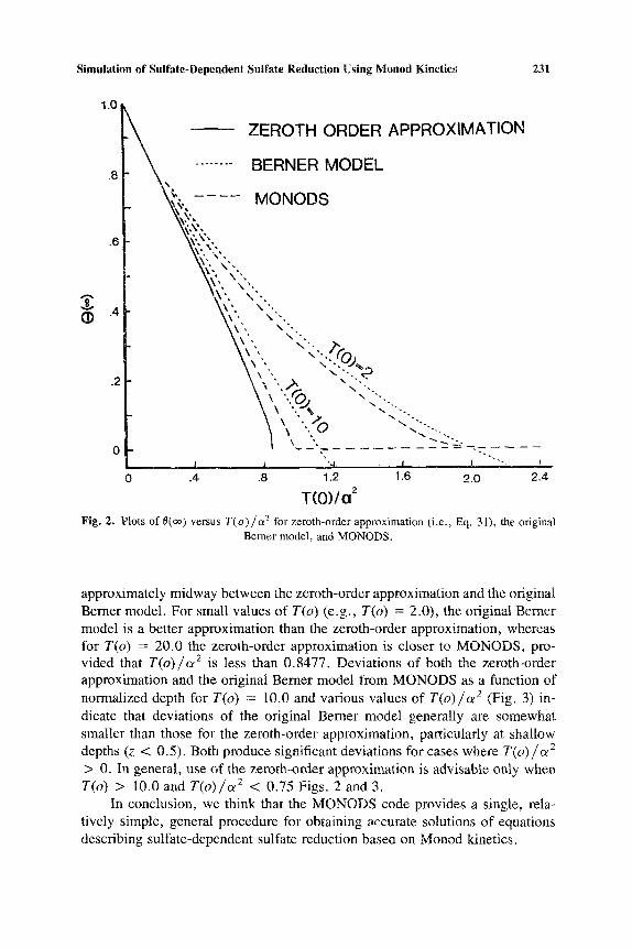
In order to compare MONODS with the zeroth approximation (Eq. 30), we have run both models using various values of T(o) and a with K = 0.05. Results show (Fig. 2) that for the zeroth-order approximation of MONODS (Eq. 31) and the original Berner model (Eq. 15) with K = 0.05, the upper limit of T(o)/2 for which Eq. 31 can produce a realistic (i.e., positive) value of 0(~) is 0.8477. Thus the zeroth-order approximation cannot be used for values of T(o)/ct 2 greater than 0.8477. Note also that MONODS and the original Bemer model both produce a family of curves depending on the value of T(o), whereas the relationship between 0(oo) and T(o) / ~ 2 for the zeroth-order approximation is defined by a single curve (i.e., Eq. 31). Clearly (Fig. 2), the zeroth-order approximation and MONODS are in closest agreement when both T(o) and c~ are large, as might be expected from Eq. 20. For T(o) = 10.0, MONODS lies


1.0

.8

ZEROTH ORDER APPROXIMATION

BERNER MODEL

MONODS

$ ®

"~,\', .6 ~,V,

,~, \%,

\ , \ ' .

.4 \ ' , \ " ,

A2 "', .,~ \ " . . \

/ " "'.,-b - ....

0 ' ~ - 4 .

0 .4 .8 1.2 1.6 2.0 2.4

T(O)/c( Fig. 2. Plots of 0(~) versus T(o)/oL z for zeroth-order approximation (i.e., Eq. 31), the original

Berner model, and MONODS.

approximately midway between the zeroth-order approximation and the original Berner model. For small values of T(o) (e.g., r(o) = 2.0), the original Berner model is a better approximation than the zeroth-order approximation, whereas for T(o) = 20.0 the zeroth-order approximation is closer to MONODS, pro- vided that T(o)/o~ 2 is less than 0.8477. Deviations of both the zeroth-order approximation and the original Berner model from MONODS as a function of normalized depth for T(o) = 10.0 and various values of T(o)/o~ 2 (Fig. 3) in- dicate that deviations of the original Berner model generally are somewhat smaller than those for the zeroth-order approximation, particularly at shallow depths (z < 0.5). Both produce significant deviations for cases where T(o)/o~ 2 > 0. In general, use of the zeroth-order approximation is advisable only when T(o) > 10.0 and T(o)/o~ 2 < 0.75 Figs. 2 and 3.

In conclusion, we think that the MONODS code provides a single, rela- tively simple, general procedure for obtaining accurate solutions of equations describing sulfate-dependent sulfate reduction basea on Monod kinetics.


. 6

.4

.2

o

a - .2

N - .4

~< - . 6

BERNER MODEL .~,7

T ~ .803 .728 .6

_ , .... .4 --

.728

.803

APPROXIMATION Z ~.8 .847

- 1 . 0 I i ~ t

0" .5 1.0 1.5 2.0

DIMENSIONLESS DEPTH Fig. 3. Plots of normalized deviations of the zeroth order approximation and original Berner model

from MONODS versus depth for T(o) = 10.0 and various values of T(o)/ot 2.

A C K N O W L E D G M E N T S

This work was supported, in part (IL), by the Industrial Associates of the Basin Analysis Group at the Universi ty o f South Carolina and in part (LRG) by NSF grant DEB-8012165. This is contribution number 646 of the Belle W. Baruch Institute for Marine Biology and Coastal Research. We wish to thank Donna Black for patiently typing the manuscript. W e also thank Drs. W. E. Sharp and B. P. Boudreau for their helpful reviews of the manuscript.

A P P E N D I X A

Mathematical Properties of Equations (19) and (20)

Physical ly, we require solutions to Eqs. (19) and (20) for which T ( z ) and O(z) are both posi t ive in oo ___ z >- 0, and for which we have the following conditions specified on z = 0

0 = 1 and T = T O on z = 0 with To > 0 and (A1)

0 = 0o (1 > 0o > 0) on z = Qo (A2)

As we will see, boundary conditions in the form (A1) and (A2) are simple to


specify and then one can infer the relevant initial slope m - d O / d z on z = 0

in terms of 0o. Because Eqs. (19) and (20) together form a third-order, nonlinear equation,

three boundary conditions are precise enough to determine the topology of the solution behavior.

By replacing T O / ( K + O) in Eq. (20) with - o t - l d T / d z from Eq. (19),

we have

620 1 dO 1 d T + - 0 (A3)

dz 2 ol dz ot dZ

which has an immediate first integral

r(z) dO _ 1 0 ( z ) + - - = constant ~ C ( 1 4 ) dz c~ c~

Inspection of Eq. (19) shows that, as long as 0 __ 0, T is a monotone- decreasing function of increasing z. Formal ly we can write

[ f z d z ' O ( z ' ) ] ( 1 5 ) T = Toexp -o~ o K + 0 ( z ' ) J

so that r ( z ) >- 0 everywhere, and i f 0 = 00(4:0) o n z = ~ , T ( z --+ ~ ) = 0. We consider two cases:

(a) 0o > 0 o n z = c ~ , i n w h i c h c a s e T = 0 o n z = ~ ;

(b) 0o = 0 on z = zc < oo, in which case we require 0 = 0 in z > Zc and

T = T= = T o e x p - o l o ( K

in z > Zc.

Case (a) O o > 0

We require 0 ~ 0o as z ~ oo; thus, d O / d z ~ 0 as z ~ ~ . The constant C in (A4) must then be -0o/O~ so that

dO/dz = e t - ' [O - Oo - T] (A6)

Consider the behavior on z = 0 where T = T O and 0 = 1. It follows from (A6) that the initial slope m ( - d O / d z ) is given by

m = o r - ' (1 - Oo - To) (AV)

As we will see, topological propert ies will force d O / d z < 0 everywhere. To anticipate this eventuali ty, write m = - n with n > 0 in (A7) so that

0 o = om + 1 - T o (A8)


Thus, if the initial slope - n is specified, we require that

To <- (1 + cm) - T, (A9)

in order that 0o be greater than zero, which constrains the allowed initial value of To in terms of the initial slope dO/dz. Note also that Eq. (A9) provides a direct connection between the initial slope and final concentration 0o at depth z

oo for any assigned value of To <- T,. Values of To > T, do not permit a physical solution.

Phase Space Behavior

We can use the first integral (A6) in Eq. (19) as follows. Write

dT dT dO dT - - - - o l - l ( o -- Oo -- T )

dz dOdz dO

It follows that

(AIO)

do_ (O-Oo: All/ dT oI2TO

Note that because T is a positive monotone-decreasing function of increasing z, it suffices to investigate properties of Eq. (Al l ) in the regime To >- T >- O. If Eq. (A11) can be solved, or the topological nature of the solution determined, we would have an explicit expression for 0 as a function of T (or T as a function of0) becauseonz = 0, T = To and0 = 1 or, o n z = oo, T = 0 a n d 0 = 0o. As far as Eq. (A11) is concerned, we are interested in that class of solutions which pass through the two points

0 = 0o on T = 0 (A12a)

0 = 1 on T = T O (A12b)

Supposing such a solution to have been found yielding T = T(O), we obtain from Eq. (A6)

f ° z = ot d O ' [ O ' - Oo - T ( O ' ) ] - ' (A13) 1

because 0 = 1 on z = 0, which completes the solution by quadrature. The main remaining problem is to solve Eq. (A11) under boundary con-

ditions (A12). Topological properties of Eq. (A11) in (0, T) space are given easily. For

T > 0, 0 > 0, note that dO/dT is everywhere positive (negative) below (above) the critical line

0 = 0o + T (A14)


A critical point o f Eq. (A11) occurs at 0 --- 0o, T = 0. Following a conventional format (Ince, 1926) in order to analyze the solution behavior of Eq. (A11) in the vicinity o f the critical point, set 0 = 0o + e with I e ] << 0o in the vicinity of T = 0 when, to lowest order in e and T, Eq. ( A l l ) reduces to

de _ _ (e - T ) ( K + 0o__ ._~ ) (A15) dT c~2TOo

with solution

= T[o~2Oo/(K + 0o) + 1 ] - ' + Go T-a (A16)

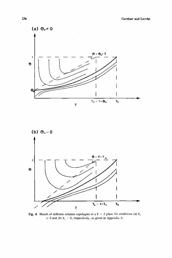
where Go is arbitrary and a = ( K + Oo)/(oflOo). For Go :~ 0, we see that solutions in the vicinity o f the critical point have a hyperbolic form, turning away from the criticat point as sketched (Fig. 4a). The exception occurs for Go = 0 when 0 approaches the critical point at 0 = 0o, T = 0, with a positive slope

0=0c [ 20o ]-, dO = 1 + ( K + 0o)j < 1 (A17)

The slope of the critical line (Eq. A14) is 1, and because the critical line also passes through the critical point 0 = 0o on T = 0, the particular solution path (on which (o = 0) approaches the critical point from below the critical line.

Only by crossing the critical line can the general solutions to Eq. (A11) change the signs o f their slopes; because all solutions (except that with Go = 0) turn away from the critical point, the solution topology is as sketched (Fig. 4a). Now all physical solutions start with T = To and 0 = 1 on z = 0. In (0, T) space, the line 0 = 1 intersects the critical line at the point 0 = 1, T c = ( 1 - 0o). But if line T = T O is to the left of line T = Tc, no solution will topologically connect from 0 = 1, T = To to 0 = 0o, T = 0. Hence, in order to have any solution, we must have

L > 1 - 0o (A18)

We already require To < T , in order to have any solution; thus To is

constrained to lie in the domain

(1 + ore) >_ To > 1 - Oo (A19)

Further: the only solution which will go to 0 = 0 o on T = 0 is the critical solution (with Go = 0) which approaches the critical point with a constant, positive, slope.

This critical solution lies everywhere below the critical line; thus it has d O / d T > 0 everywhere in T o > T > 0. But d T / d z < 0 everywhere from Eq° 19. Hence, dO/dz < 0 everywhere for the critical solution including the initial slope m ( --- - n ) .

236

( a ) (~o~ 0

Gardner and Lerche

= ~o + T

I I

I I ID

T Tc = 1 - ~ o To

(b) 0 o = 0

~//---- 3",= I+T . To / / / T

Fig. 4. Sketch of different solution topologies in a 0 - T plane for conditions (a) 0o > 0 and (b) 0o = 0, respectively, as given in Appendix A.


The initial slope n must be chosen so that we indeed are attached initially to the critical solution.

Equation (A11) cannot be solved analytically (Ince, 1926). (It can be re- written as a form of Abel 's generalized equation.) Thus, we must resort to numerical trial and error procedures in order to determine the one and only initial slope which will take the solution from 0 = 1 on T = To to 0 = 0o on T = 0 along the singular critical solution curve.

Case (b) O = O in c~ >_ z >- z¢

In this case, integration o f Eq. (20) across an infinitesimally small domain surrounding z = Zc forces us to the requirement that dO/dz is continuous across z - zc. Because 0 -- 0 in z >- Zc, the required boundary conditions on the equation are now

0 = 1 T = T o on z = 0

0 = 0 dO/dz = 0 T = T~ < T O on z = zc

T = T= and 0 = 0 i n z > z~

From Eq. (A4), constant C must be Too/o~ so that

dO/dz = o~-1[0 - ( T - Too)] (A20)

On z = 0, the initial slope m ( - d O ~ & ) is given by

m = c~-1[1 - (To - T~)] ( 1 2 1 )

Again we have to wait until after a determination of the topological properties of the solution behavior to see if slope dO/dz is everywhere o f one sign.

Phase Space Behavior

We again use the first integral in Eq. (19) to write

dO [0 - ( T - Too)] (K + O) d T - o~2T0 in z < Zc (A22)

From Eq. (A5), d T / d z is a positive monotone-decreasing function of increasing z in 0 < z - zc so that it suffices to investigate the properties of Eq. (A22) in the regime T o _ T _> Too > 0. An investigation o f the topological solution properties of Eq. (A22) follows the same road as in the previous case. For T > T~o, note that d O / d T is everywhere positive (negative) below (above) a critical line

0 = ( T - T~) (123 )

1 critical point of Eq. (122) occurs at 0 = 0, T = T~. Following the usual


format (Ince, 1926) in order to analyze the solution behavior of Eq. (A22) in the vicinity o f the critical point, set T = T~ + 6 with 16[ < < T~ in the vicinity of 0 = 0 when, to lowest order in 0 and 6, Eq. (A22) reduces to

dO = - [0 - 61K (A24) d6 otZToo6

with solution

0 = 611 + (c~2Toolg)] -1 + ~o 6-x/~zr~ (A25)

where ~'o is arbitrary. For ~'o ~e 0, solutions in the vicinity of the critical point have a hyperbolic form, turning away from the critical point as shown (Fig. 4b). The exception occurs for ~'o = 0 when 0 approaches the critical point at 0 = 0, T = Too with a positive slope

dO = 1 + - - < 1 ( 1 2 6 ) ~ T=T~

Because the slope of the critical line is 1 and because the critical line also passes through the critical point 0 = 0 on T = T~, this particular solution path (on which ~'o = 0) approaches the critical point from below the critical line.

Again we see that because the general solutions can change the signs of their slopes only by crossing the critical line and because all solutions (except that with ~'o = 0) turn away from the critical point, the solution topology in zo >- z -> 0 is as sketched (Fig. 4b). Note that on the critical solution curve, passing through the critical point, we have d O / d T > 0 everywhere in zc > z > 0. Because d T / d z < 0 everywhere in zc > z >- 0, it follows that dO/dz <

0 in the same domain. Hence, 0 is a positive monotone-decreasing function of increasing z in Zc -> z -> 0.

In (0, T) space, the line 0 = 1 intersects the critical line 0 = (To - T~)

o n

T. = 1 + T~ (127 )

But if line T = T O is to the left of line T = T., no solution will topologically connect from 0 = 1, T = T O to 0 = 0, T = T~ on z = ze. Hence, in order to have any solution, T O must be to the right of T,; i.e., we must have

To > 1 + Too (A28)

in order that any solution exist. Expressing the point slightly differently: If 0 does indeed tend to zero at a

finite ze, then that value of z~ must be such that inequality (A28) is necessarily satisfied or no solution extending from z = 0 to z = Zc will exist.

Again we see that if inequality (A28) is satisfied, the initial slope m in Eq.


(A21) is negative as required by the topology of the solution curves. We also are faced once more with the numerical task of scanning through initial slopes until we determine that unique slope which will guarantee that we are indeed locked on to the single critical solution which goes smoothly from 0 -- 1, T = T o on z = 0 to the critical point at z = zc where 0 = 0, T = To~. Thus, we are again faced with a t r ial-and-error search for that " m a g i c a l " initial slope.

REFERENCES

Bagander L. E., 1977, In Situ Studies of Bacterial Sulfate Reduction at the Sediment-Water Inter- face, in Sulfur Fluxes at the Sediment-Water Interface--an In Situ Study of Closed Systems, En and pH: Department of Geology, University of Stockholm, Publication no. 1, p. 1-30.

Berner, R. A., 1964, An Idealized Model of Dissolved Sulfate Distribution in Recent Sediments: Geochim. Cosmochim. Acta, v. 28, p. 1497-1503.

Boudreau, B. P. and Westrich, J. T., 1984, The Dependence of Bacterial Sulfate Reduction on Sulfate Concentration in Marine Sediments: Geochim. Cosmochim. Acta, v. 48, p. 2503- 2516.

Hallberg, R. A.; Bagander, L. E.; and Engvall, A. S., 1976, Dynamics of Phosphorus, Sulfur and Nitrogen at the Sediment-Water Interface; in J. O. Nriagy (Ed.), Environmental Biogeochem- istry: Ann Arbor Science Publishing, Michigan, p. 295-308.

Ince, E. L., 1926, Ordinary Differential Equations: Longmans, Green and Co., London. p. 558. Jorgensen, B. B., 1983, Tile Microbial Sulfur Cycle, in W. E. Kmmbein (Ed.) Microbial Geo-

chemistry: Academic Press, New York, p. 91-124. Lentini, M. and Pereyra, U., 1977, An Adaptive Finite-Difference Solver for Nonlinear Two-Point

Boundary Problems with Mild Boundary Layer: Soc. Indus. Appl. Math. J. Numer. Anal., v. 14, p. 91-111.

Martens, C. S. and Berner, R. A., 1977, Interstitial Water Chemistry of Anoxic Long Island Sound Sediments. I. Dissolved Gases: Liminol. Oceanogr. v. 22, p. 10-25.

Monod, J., 1949, The Growth of Bacterial Cultures: Ann. Rev. Microbiol., v. 3, p. 371-394. Ramm, A. E. and Bella, P. A., 1974, Sulfide Production in Anaerobic Microcosms: Liminot.

Oceanogr., v. 19, p. 425-441. Speckhart, T. H. and Green W. L., 1976, A Guide to Using CSMP--The Continuous Systems

Modeling Program: Prentice-Hall, Englewood Cliffs, New Jersey, p. 325.

simulation of sulfate-dependent sulfate reduction using monod kinetics

Documents