ORIGINAL RESEARCH

Simulation of Stochastic differential equation of geometricBrownian motion by quasi-Monte Carlo methodand its application in prediction of total index of stock marketand value at risk

Kianoush Fathi Vajargah1 • Maryam Shoghi1

Received: 2 February 2015 / Accepted: 22 May 2015 / Published online: 24 June 2015

� The Author(s) 2015. This article is published with open access at Springerlink.com

Abstract In the prediction of total stock index, we are

faced with some parameters as they are uncertain in future

and they can undergo changes, and this uncertainty has a

few risks, and for a true analysis, the calculations should be

performed under risk conditions. One of the evaluation

methods under risk and uncertainty conditions is using

geometric Brownian motion random differential equation

and simulation by Monte Carlo and quasi-Monte Carlo

methods as applied in this study. In Monte Carlo method,

pseudo-random sequences are used to generate pseudo-

random numbers, but in quasi-Monte Carlo method, quasi-

random sequences are used with better uniformity and

more rapid convergence compared with pseudo-random

sequences. The predictions of total stock index and value at

risk by this method are better and more exact than Monte

Carlo method. This study at first evaluates random differ-

ential equation of geometric Brownian motion and its

simulation by quasi-Monte Carlo method, and then its

application in the predictions of total stock market index

and value at risk can be evaluated.

Keywords Geometry Brownian motion � Quasi-Monte

Carlo simulation � Sobol quasi-random sequence �Value at risk

Introduction

Like other fields of management knowledge and its appli-

cation, risk management applies knowledge, principles,

and specific rules to estimate predictions and achieve pre-

defined goals. This field aims to help in ensuring the con-

tinuous protection of the people, and in safeguarding their

assets and activities against the adverse events, as histori-

cally they are associated with risk.

In Iran, for 14 years, this issue has been paid serious

attention. To fulfill the 20-year vision of Islamic Republic

of Iran and to fulfill the development goals, the manage-

ment and planning organization of the country emphasizes

the effective implementation of plans by means of evalu-

ations of economic and technical methods, and project

management system by means of new management prin-

ciples such as value engineering and risk management.

One of the famous methods to measure, predict, and

manage risk is value at risk (VAR) that has been receiving

great attention in recent years of managers of capital

markets of various countries. VAR is a statistical criterion

presenting quantitatively the maximum probable portfolio

loss incurred during a definite period [5].

The calculation of VAR is done by two methods:

parametric and nonparametric. In the parametric method,

the main hypothesis is the normality of distribution of

return on asset, and it is not an ideal hypothesis for

application under real and practical conditions. As assets

do not follow normal distribution under these conditions,

this study applies nonparametric and Monte Carlo and

quasi-Monte Carlo simulation techniques. In this method,

by simulation of samples through computer and MATLAB

software and random differential equation of geometric

Brownian motion, the prediction is performed. The study

aimed to evaluate the performance of Monte Carlo and

& Kianoush Fathi Vajargah

k_fathi@iau-tnb.ac.ir

1 Department of Statistics, Islamic Azad University, North

Branch Tehran, Tehran, Iran

123

Math Sci (2015) 9:115–125

DOI 10.1007/s40096-015-0158-5

quasi-Monte Carlo simulation methods to calculate total

index and VAR of stock market to quantify the maximum

probable loss with the lowest percentage error for the

investment in stock market by considering the volatilities

in the market.

This issue is of great importance for stock managers.

In recent years, by introducing VAR as a tool to cal-

culate risk and Monte Carlo and quasi-Monte Carlo sim-

ulation techniques, various researches have been

conducted, and some of them are described hereunder.

Giles et al. [2] in their study showed that quasi-Monte

Carlo method in financial calculations is better than Monte

Carlomethod as the former can achieve similar precisionwith

lower calculation cost, and their study refers to three impor-

tant components of Sobol sequence and network points:

dimension effect reduction by principal component analysis

(PCA); random selection to present nonbiased estimatorswith

a definite confidence interval; and the application of Brown-

ian motion and Brownian bridge in their calculations.

Huang [3] applied Monte Carlo simulation method and

Brownian motion to calculate VAR and obtained optimal

VAR by adjustment coefficient, and his study results

showed that optimal VAR was efficient and estimated the

maximum expected loss with high confidence interval. In

this paper, we begin with considering the review of the

literature followed by the theoretical basics of study. Next,

a comparison is made between quasi-random sequences

and pseudo-random sequences, then definitions of the

terms that are used regarding stock market are given, and

finally conclusions are drawn.

Brownian motion

Let (P, X, A) be a probability space. In a random process,

Wt: X ? R, {W(t), � B t B T} is called a Brownian

motion, if the following conditions are satisfied:

1. For all X 2 x, t ? Wt(x) is a continuous function on

[0, T] interval.

2. Each group of {W(t�), W(t1) - W(t�), W(t2) -

W(t1), …, W(tk) - W(tk-1)}intervals with 0 B t0\ t1\ ���\ tk B T is independent.

3. For each � B s\ t B T, we have

W ðtÞ �W ðsÞ ! N ð� ; t � sÞ ð1Þ

Based on above properties, we can say for each

�\ t B T, we have W(t) * N(�, t).

d-dimensional Brownian motion

Let (P, X, A) be a probability space and d 2 N. In random

process, Wt: X ? R, {W(t), � B t B T} is called

d-dimensional Brownian motion, if the following condi-

tions are satisfied:

1. For all, x X 2, t ? Wt(x) is a continuous function on

[�, T] interval.2. Each group of {W(t�), W(t1) - W(t�), W(t2) -

W(t1), …, W(tk) - W(tk-1)} intervals, by assuming

0 B t0\ t1\ ���\ tk B T, is independent.

3. For each � B s\ t B T, we have

W ðtÞ �W ðsÞ ! N ð� ; ð t � sÞIdÞ ð2Þ

Brownian motion is also called a Standard Brownian

Motion, if the following equation is established definitely:

W0 = 0.

As long as Brownian motion can have negative values,

its direct use is doubtful for modeling the stock prices.

Thus, we introduce a nonnegative type of Brownian motion

called Geometric Brownian Motion. Geometric Brownian

motion is always positive as the exponential function has

positive values. Geometric Brownian Motion is defined as

S(t) = S0 eX(t), where X(t) = rW(t) ? lt is a Brownian

motion with deviation, S(0) = S0[ 0

Taking logarithm of the above equation, we have

X tð Þ ¼ ln s tð Þ=s0ð Þ ¼ ln s tð Þð Þ� ln s0ð Þ ! ln s tð Þð Þ¼ ln s0ð Þ þ X tð Þ

Thus, ln (s(t)) has normal distribution with mean ln

(s0) ? lt and variance r2t, and for each t value, s(t) has

normal log distribution [10].

If we let �r ¼ lþ r22;E s tð Þð Þ ¼ e�rts0 and �r � r where

r is the share growth rate under risk-free conditions as

investment in banks, and �r is the share growth rate

under risk conditions as investment in stock market,

then �r is the share growth rate under risky conditions

as investment in stock market. The share growth rate

under risky conditions should be much more than that

under risk-free conditions to motivate the investors to

investment.

Theorem 2.1 At constant time t, geometric Brownian

motion has normal log distribution with mean ln (s0) ? ltand variance r2t.

Proof

F xð Þ ¼ P X� xð Þ ¼ P s0esp lt þ rW tð Þð Þ � xð Þ¼ P lt þ rW tð Þ� ln x=s0ð Þð Þ¼ P W tð Þ� ln x=s0ð Þ � ltð Þ=rð Þ¼ P W tð Þ

� ffiffit

p� ln x=s0ð Þ � ltð Þ

�r

ffiffit

p� �� �

¼Z ðln x=s0ð Þ�ltÞ=ðr

ffiffit

pÞÞ

�1

1ffiffiffiffiffiffi2p

p exp � y2

2

� �dy

If we calculate the derivative of the above equation with

respect to X, then we have

116 Math Sci (2015) 9:115–125

123

f ðxÞ ¼ 1ffiffit

pxr

ffiffiffiffiffiffi2p

p e�12ð Þ ln xð Þ�lnðs0Þ�ltð Þ=ðr

ffiffit

pÞð Þ2

� �

For 0 = t0\ t1\ ���\tn = t, ratios 1� i� n; Li ¼ sðtiÞsðti�1Þ,

random independent variables of log are normal, indicating

the percent changes of the share value as it is not inde-

pendent of real changes. sðtiÞ � sðti�1Þ:For example:

L1 ¼ sðt1Þsðt0Þ

¼ exðt1Þ L2 ¼ sðt2Þsðt1Þ

¼ exðt2Þ � exðt1Þ

are independent and normal log, and x(t1) and x(t2) - x(t1)

are independent with normal distribution. Now, we can

rewrite geometric Brownian motion as S(t) = S0 L1 L2 …Ln as an n-variate normal log. For example, assume that we

sample share value at the end of each day. We can use

ti = I, and thus, we have Li ¼ sðiÞsði�1Þ which shows the per-

cent of change during a day. Now, we can use the above

formula in this regard. When for each i, ti - ti-1 = 1, Li is

distributed uniformly, ln (Li) has normal distribution with

mean l and variance r2.Geometric Brownian motion not only solves negation

problem, but based on basic economic principles, it is also

considered as a good model for stock value. As stock price

reacts rapidly to new information, geometric Brownian

motion model as Markov process is used for it.

If a geometric Brownian motion is defined with differ-

ential equation dS ¼ rS dt þ rS dW ; S 0ð Þ ¼ s0, then geo-

metric Brownian motion is equal to:

S tð Þ ¼ s0 exp r � 1

2r2

� �t þ rW tð Þ

� �

As geometric Brownian motion has normal log distri-

bution with parameters ln s0ð Þ þ rt � 12r2t and r2t; the

mean and variance of geometric Brownian motion are

given by

E S tð Þð Þ ¼ s0 exp rtð Þ

Var S tð Þð Þ ¼ s20e2rt er

2t � 1� ð3Þ

If the main issue is geometric Brownian motion

S(t) = s0 exp (lt ? rWt), then its random differential

equation formula is as follows:

dS ¼ l þ 1

2r2

� �S tð Þdt þ rS tð Þ dW ; Sð0Þ ¼ s0

As geometric Brownian motion has normal log distri-

bution with parameters ln (s0) ? lt and r2t, the mean of

geometric Brownian motion is equal to s0 exp lt þ 12r2t

� �;

and its variance is as per the following formula:

Var S tð Þð Þ ¼ s20e2ltþr2t er

2t � 1�

ð4Þ

[10].

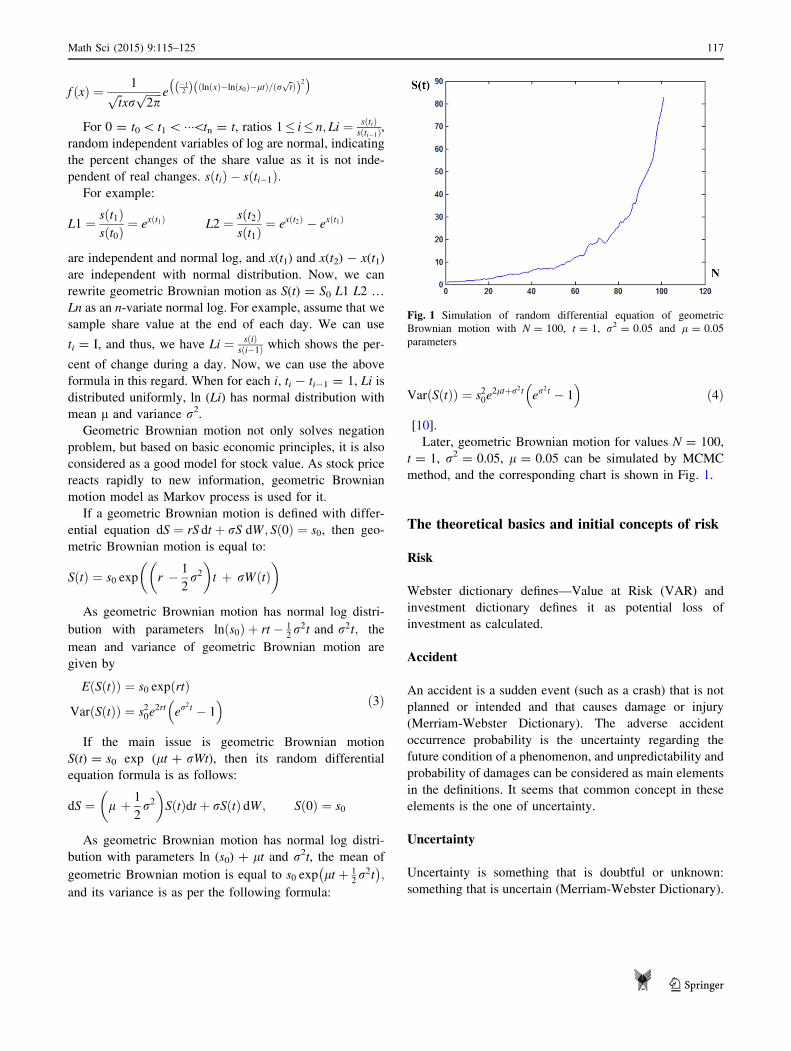
Later, geometric Brownian motion for values N = 100,

t = 1, r2 = 0.05, l = 0.05 can be simulated by MCMC

method, and the corresponding chart is shown in Fig. 1.

The theoretical basics and initial concepts of risk

Risk

Webster dictionary defines—Value at Risk (VAR) and

investment dictionary defines it as potential loss of

investment as calculated.

Accident

An accident is a sudden event (such as a crash) that is not

planned or intended and that causes damage or injury

(Merriam-Webster Dictionary). The adverse accident

occurrence probability is the uncertainty regarding the

future condition of a phenomenon, and unpredictability and

probability of damages can be considered as main elements

in the definitions. It seems that common concept in these

elements is the one of uncertainty.

Uncertainty

Uncertainty is something that is doubtful or unknown:

something that is uncertain (Merriam-Webster Dictionary).

Fig. 1 Simulation of random differential equation of geometric

Brownian motion with N = 100, t = 1, r2 = 0.05 and l = 0.05

parameters

Math Sci (2015) 9:115–125 117

123

Risk dimensions

Productive and unproductive risk

Productive risk is the one assuring value added, but

unproductive risk is without value added (investment in

mine exploration project includes productive risk of eco-

nomic type, but attending gambling, for example, where

risking one’s property to achieve much greater money, is

called unproductive risk).

Controllable and uncontrollable risk

Controllable risk can be controlled by decision maker,

while in uncontrollable risk, the decision maker has no

control on risk (controllable risk is called reactive risk, and

uncontrollable risk is called chance risk).

Profit-and-loss risk

Risk is divided into real (net) risk and involves winning

and losing. The real risk includes loss (as car owner incurs

damage in case of accident; otherwise it is not changed),

and speculative risk includes loss and profit (its good

example is the ownership of a factory or company). Simply

put, risk can include loss (negative risk) and profit (positive

risk) [1].

Different types of risks

There are different types of risks, and some of them are

explained briefly.

Market risks

Market risk refers to the risk of losses in the bank’s trading

book due to changes in equity prices, interest rates, credit

spreads, foreign-exchange rates, commodity prices, and

other indicators values of which are determined by variable

factors in a public market [7].

Exchange rate risk

The exchange rate risk is defined as the variability of a

firm’s value due to uncertain changes in the rate of

exchange [4].

Inflation risk

Unexpected inflation is a change in prices that differs from

the consensus view of what inflation is expected to be.

When we talk about inflation risk, we are commonly

talking about unexpected inflation. While expected infla-

tion must be planned for in retirement budgeting, unex-

pected inflation causes uncertainty in prices, because it

causes an element of surprise to bear upon the market.

Since it cannot be predicted, managing the risk of unex-

pected inflation is critical [8].

Value at risk

Value at risk (VAR) as a statistical criterion defines the

maximum expected loss of keeping assets in definite period

and at definite confidence level. Assume that the daily

value of an asset is 200 million Toman and at probability of

99 %, it is possible that the maximum reduction of this

asset on the next day be 10 million Toman. Thus, VAR of

this asset in a period of one day at a confidence interval of

99 % is 190 million Toman. We can say that by confidence

interval of 99 %, the value of this asset on the next day will

not be not less than 190 million Toman.

From math issues, VAR is shown as

Prob dV � � VaRf g� a; ð5Þ

where dV is the change of asset value in a definite period

The above equation states that the probability of the

asset loss in future period being less than VAR is 1 - a[11] (Fig. 2).

In financial sciences, it is assumed that random variables

price follows the path depending on Brownian motion as

stock price, and one of its common models is geometric

Brownian motion.

Fig. 2 Value at risk (risk analytics site)

118 Math Sci (2015) 9:115–125

123

Monte Carlo Method

For a given population L, a parameter, e.g., h, is estimated.

In the Monte Carlo method, an estimate detector S(x) is

first determined, in which x is a random variable with

density function fx(x).

The estimate detector should satisfy the following two

conditions:

(A) The estimate detector should be unbiased.

E SðxÞ½ � ¼ h

(B) The estimate detector should have definite variance.

var S xð Þð Þ ¼ r2

Regarding the random samples X1…. NN of the function,

density of fx(x) is used.

hN X1. . .XNð Þ ¼ 1

N

XN

n¼1

SðXnÞ ð6Þ

varðhNÞ ¼r2

N\1; E hN

� ¼ h

We assume estimator number [6] as Monte Carlo esti-

mator [6].

Monte Carlo simulation and stochastic differential

equation

In this simulation, we present the expected value

E[g(X(T))] for a solution, X, of a known stochastic differ-

ential equation with a known function of g. In general,

bipartite approximation error contains two parts: random

error and time discretization error. Statistical error estimate

is based on the central limit theorem. Error estimation for

the time-discretization error of the Euler method directly

measures with one remained phrase the accuracy of 12

robust approximation.

Consider the following stochastic differential equation:

dX tð Þ ¼ a t;X tð Þð Þ þ b t;X tð Þð ÞdWðtÞ:

How can the value of E[g(X(T))] be calculated on

t0 � t� T . Monte Carlo method is based on the approxi-

mation of

E g X Tð Þð Þ½ � ffiXN

j¼1

g �X T;xj

� �� �

N

where X is an approximation of X; according to Euler

method, the error in the Monte Carlo method is

E g X Tð Þð Þ½ � �XN

j¼1

g �X T ;xj

� �� �

N

¼ E g X Tð Þð Þ � g �X Tð Þð Þ½ �

�XN

j¼1

g �X T ;xj

� �� �� E g �X Tð Þð Þð ÞN

:

Quasi-Monte Carlo (QMC)

The basic concept of quasi-Monte Carlo method is based

on moving the random sample in Monte Carlo method with

definite points accurately. The criterion of selection of

definite points is that the sequence in [0,1)s has better

uniformity than a random sequence. Indeed, these points

should be such that [0,1)s is covered uniformly. To mea-

sure uniformity, a different concept is used as explained in

the following definitions.

Definition 7.1 (estimation of quasi -Monte Carlo)

Assume X1, …, XN is selected of [�, 1)s space, estimation

of quasi-Monte Carlo is done as per the formula:

�IQMC ¼ 1N

PNi¼1 f ðXiÞ.

In an ideal model, we replace the set of x1,…, xn points

with infinite sequence x1, x2,… in [0,1)s. A basic condition

for this sequence is that the term limN!1

1N

PNn¼1 f ðXnÞ ¼

R½� ; 1Þs f ðxÞdx is satisfied.

The satisfaction of this term is achieved as sequence x1,

x2, …, xn is distributed uniformly in [0,1)s. The difference,

deviation scale of uniformity, is a sequence of points in

[0,1)s.

Definition 7.2 (uniform distribution in [�, 1)s) {Xn}n2Nsequence is distributed uniformly in [�, 1)s if for each

x 2 d[�, 1)s, we have

limN!1

1

N

XN

n¼1

f ðXnÞ ¼Z

½� ; 1Þsf ðxÞdx ¼ I

Definition 7.3 (general discrepancy) Assume p is a set of

points {X1, …, XN}, and B is the family of subsets B 2[�, 1)s. Then, the general discrepancy of set of points

p = {X1, …, XN} in interval [�, 1)s is as follows:

DNðB; pÞ ¼ supB

PN

n¼1

CBðXnÞ

N

� ksðBÞ

ð7Þ

where DN(B, p) is always between [0, 1], and CB isan

attribute function of B. Thus,PN

n¼1 CBðXnÞ shows the

number of points 1 B n B N and xn e B.

Math Sci (2015) 9:115–125 119

123

Definition 7.4 (Star discrepancy) Assume J* is the family

of all sub-intervals [�, 1)sasQs

i¼1½�; uiÞs; �\ui � 1. The

star discrepancy of the set of p = {X1,…, XN} on substi-

tuting with J* in place of B in Eq. [6] is as follows:

DN ¼ DNðJ;PÞ ¼ sup

BeJ

PN

n¼1

CBðXnÞ

N� kðBÞ

: ð8Þ

Theorem 7.1 (Koksma Inequality) If f has bounded

changes v(f) in [0, 1], then for each set of p = {X1, …, XN}

of [0, 1], we have

PNn¼1 f ðXnÞN

�Z 1

�f ðxÞdx

� vðf ÞD

NðpÞ

This inequality states that sequences with low discrep-

ancy lead to low error [9].

In Monte Carlo method, there was an aggregation of

points as the points were independent, and they had no

awareness of each other, and there was little chance that

they were very close to each other. Quasi-random

sequences had better uniformity and rapid convergence

compared with pseudo-random sequence. Some of the

quasi-random sequences are mentioned later, and they are

calculated by means of MATLAB software.

Van der corput sequence

This is the first sequence by which low discrepancy was

formed.

To obtain the nth point of this sequence, at first, n on

base b is defined as n ¼Pm

j¼� aj nð Þb j where coefficients

aj(n) include {�, 1,…, b - 1}values. We use these coef-

ficients to achieve quasi-random values as

Xn ¼ /bðnÞ ¼Pm

j¼� ajðnÞ 1bjþ1. Some of aj(n) values are

nonzero. M is the smallest integer for each j[m as

aj(n) = 0 (Table 1).

Table 1 Calculation of ten first

points of Van der corput

sequence in basis 3

n 1 2 3 4 5 6 7 8 9 10

u3(n) 0.333 0.666 0.111 0.444 0.777 0.222 0.555 0.888 0.037 0.370

Table 2 Calculation if first five points of Halton sequence for first

four dimensions

n u1(n) (base 2) u2(n) (base 3) u3(n) (base 5) u4(n) (base 7)

1 0.500 0.333 0.200 0.142

2 0.250 0.666 0.400 0.285

3 0.750 0.111 0.600 0.428

4 0.125 0.444 0.800 0.571

5 0.625 0.777 0.040 0.714

Fig. 3 Halton sequence for 1, 2 and 14, 15 dimensions

120 Math Sci (2015) 9:115–125

123

Van der corput sequence is a unidimensional sequence

and generates random data of this sequence; in high

dimensions, they can lose their random state and follow a

linear function.

Halton sequence

Halton sequence was proposed in 1960, and it is similar to

Van der corput sequence. First dimension of Halton

sequence is a Van der corput sequence in basis 2, and

second dimension is a Van der corput sequence in basis 3.

Indeed, we can say Halton sequence is the same as Van der

corput sequence with basis value as the nth primary value

for the nth dimension of Halton sequence. Halton sequence

is a s-dimensional sequence in cubic [0, 1]s. Nth element of

Halton sequence in [0, 1]s is defined as (Table 2)

xn ¼ /b1ðnÞ;/b2

ðnÞ; . . .;/bsðnÞ

� �n ¼ �; 1; 2; . . .

ð9Þ

Figure 3 shows 100 Halton sequences in bases 2, 3 and

dimensions 1, 2 (right figure); and bases 43, 47 and

dimensions 14, 15 (left figure). As shown, in low dimen-

sion, Halton sequence has suitable dispersion, but by

increasing the dimension, convergence is revealed as in

high dimensions, its random trend is lost and hypercube is

not covered uniformly.

Sobol sequence

Sobol sequence was proposed in 1967. Constant value of

basis 2 is used in Sobol sequence for all dimensions. Thus,

Sobol sequence is rapid and simpler. This feature generates

random numbers with low convergence in high

dimensions.

To make this sequence, at first, we write n for basis 2

according to n ¼PM

i¼� ai2i as M is the smallest value

Table 3 Calculation of first 5 points of Sobol sequence for first 5

dimensions

n Dim = 1 Dim = 2 Dim = 3 Dim = 4 Dim = 5

1 0.500 0.500 0.500 0.500 0.500

2 0.250 0.750 0.250 0.750 0.250

3 0.750 0.250 0.750 0.250 0.750

4 0.125 0.625 0.875 0.875 0.625

5 0.625 0.125 0.375 0.375 0.125

Fig. 4 Sobol sequence for 1, 2 and 14, 15 dimensions

Table 4 The comparison of quasi-random sequences and pseudo-random sequences in integral evaluation (N = 100)

Pseudo-

random

sequences

Halton sequence

in dimension 1

and basis 2

Sobol sequence

in dimension 1

and basis 2

Halton sequence

in dimension 10

and basis 29

Sobol sequence

in dimension 10

and basis 2

Approximate value integralR 1

0exp xð Þdx 1.7696 1.7195 1.7195 1.7474 1.7044

Integrating error 0.0513 0.0012 0.0012 0.0291 -0.0139

Math Sci (2015) 9:115–125 121

123

bigger or equal to logn2 and ais values are zero or one,

respectively.

The primary polynomial rank q is assumed as

p = xq ? c1xq-1 ? ��� ? cq-1x ? 1 in which cis values

are zero and one. mi by coefficients ci are generated as

follows:

mi ¼ 2c1mi�1 22c2mi�2 � � � 2q�1cq�1mi�qþ1

2qmi�q mi�q ð10Þ

As is an operator in computer represented as 1 � ¼� 1 ¼ 1 1 1 ¼ � � ¼ � mi values are odd integer

values in interval [1, 2i - 1]. V(i)s are generated according

to V ið Þ ¼ mi

2i:

Thus, nth element of Sobol sequence is generated

according to /(n) = a�v(1) a1v(2) ��� ai-1v(i).

To facilitate Sobol sequence generation, Grey code

coding is used, and its algorithm is given by /ðnÞ ¼ n n2;

and now the adjusted model is given by /ðnÞ ¼ n n2

(Table 3).

Figure 4 shows 100 points of Sobol sequences in

dimensions 1, 2 (right figure) and dimensions 14, 15 (left

figure). As shown, in high dimensions, this sequence has

good uniformity and it makes its advantage compared to

other sequences.

Comparison of quasi-random and pseudo-randomsequences

Integral evaluation

To show which method is effective on integral evaluation,R 1

0expðxÞ dx is considered. The exact answer of this inte-

gral is 1.7183. Table 4 shows the calculation of this inte-

gral by Monte Carlo and quasi-Monte Carlo method, and

the integrating error is calculated.

As shown in Table 4, quasi-random sequences in inte-

gral evaluation perform better than pseudo-random

sequences, and their estimation error is low. As was stated

earlier, Sobol sequence in high dimensions is more efficient

than Halton sequence.

Uniformity

The higher the uniformity of sequences, the lower the

calculation error, and the sequence covered interval 0 to 1

very well. Table 5 shows a series of statistical features of

Monte Carlo and quasi-Monte Carlo sequences in com-

parison with Uniform distribution.

As shown in Table 5, statistical features of quasi-ran-

dom sequences are closer to uniform distribution [0, 1] than

Table 5 Comparison of quasi-random sequences and pseudo-random

sequences with uniform distribution [0, 1] (N = 500)

Uniform

distribution

[0, 1]

Pseudo-

random

sequence

Halton

sequence in

dimension 3

and basis 5

Sobol

sequence in

dimension 30

and basis 2

Mean 0.5000 0.4942 0.4984 0.5000

Variance 0.0833 0.0795 0.0835 0.0833

Skewnessa 0.0000 0.0401 0.0000 0.0000

Kurtosisb 1.8000 1.8283 1.7999 1.8005

Min 0.0000 0.0012 0.0000 0.0000

Max 1.0000 0.9991 0.9968 1.0000

a g1 ¼PN

i¼1yi��yð Þ3=Ns3

b g2 ¼PN

i¼1yi��yð Þ4=Ns4

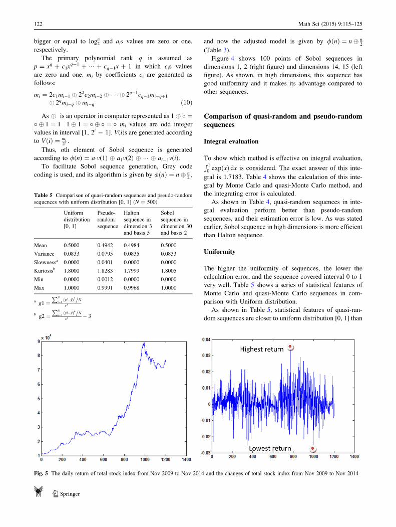
� 3

Fig. 5 The daily return of total stock index from Nov 2009 to Nov 2014 and the changes of total stock index from Nov 2009 to Nov 2014

122 Math Sci (2015) 9:115–125

123

pseudo-random sequence. It means that quasi-random

sequences are mostly representing U[0, 1] than pseudo-

random sequence. As was said before, these sequences are

associated with low discrepancy, their interval [0, 1] cov-

erage is better, and are much more uniform. Also, Sobol

sequence is more uniform than Halton sequence.

Nonconference of sequence in high dimensions

As shown in Fig. 3, by increasing dimension, convergence

of Halton sequence is increased, and its trend of randomness

is lost. Halton sequence has low convergence compared

with Van der corput sequence in high dimensions. Sobol

sequence as shown in Fig. 4 performs better than other

quasi-random sequences as it applies basis 2 for all

dimensions, and it leads to low convergence and high speed.

To predict total stock market index and calculation of

VAR, a total index of 5 continuous years (Nov 2009–Nov

2014) was extracted from stock organization site, and it is

equal to 1204 as the number of working days in these

5 years in Iran (Fig. 5).

As shown in Table 6, kurtosis of return is high, and it

indicates that the total stock index distribution of TSE is far

from normal value, and because of this, we applied Monte

Carlo and quasi-Monte Carlo simulation methods, and

these methods do not require normal distribution.

To obtain the prediction values of total TSE index and

calculation of VAR, the following stages are considered:

1. Determining time interval as one day (dt = 1).

2. Generation of random numbers by Monte Carlo and

quasi-Monte Carlo method and putting them in random

differential model of geometric Brownian motion Si ¼ðSi� 1þ Si� 1 r dt þ r e

ffiffiffiffidt

p� �Þ to predict total index.

Table 6 The statistical features of total stock index of TSE

Min Max Kurtosis Skewness Variance Mean

-0.0276 0.0344 4.0900 0.1444 0.00005 0.0015

Fig. 6 100,000 simulation paths of total TSE index for 10 days by

Monte Carlo method

Fig. 7 Total TSE index and VAR calculated by Monte Carlo method

Fig. 8 100,000 simulation paths of total TSE index for 10 days by

quasi-Monte Carlo

Fig. 9 Total TSE index and VAR calculated by quasi-Monte Carlo

method (Sobol sequence)

Fig. 10 Total TSE index and VAR calculated by quasi-Monte Carlo

method (Halton sequence)

Math Sci (2015) 9:115–125 123

123

For Stage 2 for a period of 10 days (according to Bazel

committee in Swiss), simulation is performed M times,

and this value is equal to 100,000 in this study.

3. Sorting total predicted indices of small to big and

calculation of its first percentile to determine the VAR

at confidence interval of 99 %.

4. Stages 2, 3 are performed L times. As shown in this

study, moving window approach is used. This means

that first window includes 1000 first data, and the

model applies these data to predict 1001 data. In the

next stage, the window considers data 2 to 1001, and

the model applies these data for prediction of 1002

data, and this window moves forward (L = 193) to

include 1000 final data. As some(same) values are

predicted by this method and as we have their real

values, we can evaluate the validation of the model by

determining prediction error (Fig. 6).

As shown in Fig. 7, in some cases, VAR is not predicted

precisely, and TSE total index is lower than the maximum

loss (Fig. 8).

As shown in Figs. 9 and 10, VAR is predicted accu-

rately by quasi-Monte Carlo method, and the two sequen-

ces showed good results as one dimension is used for

prediction.

As shown in Table 7, VAR error ratio calculated by

Monte Carlo method is 0.05; with higher than 0.01 as the

probable error level, this method estimates low values of

risk, and this leads to inadequacy of capital to resist against

risk.

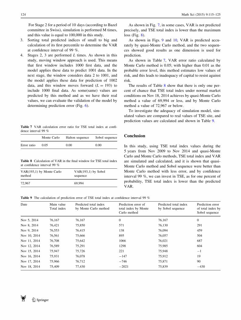
The results of Table 8 show that there is only one per-

cent of chance that TSE total index under normal market

conditions on Nov 18, 2014 achieves by quasi-Monte Carlo

method a value of 69,994 or less, and by Monte Carlo

method a value of 72,967 or below.

To investigate the adequacy of simulation model, sim-

ulated values are compared to real values of TSE site, and

prediction values are calculated and shown in Table 9.

Conclusion

In this study, using TSE total index values during the

5 years from Nov 2009 to Nov 2014 and quasi-Monte

Carlo and Monte Carlo methods, TSE total index and VAR

are simulated and calculated, and it is shown that quasi-

Monte Carlo method and Sobol sequence were better than

Monte Carlo method with less error, and by confidence

interval 99 %, we can invest in TSE, as for one percent of

probability, TSE total index is lower than the predicted

VAR.

Table 8 Calculation of VAR in the final window for TSE total index

at confidence interval 99 %

VAR(193,1) by Monte Carlo

method

VAR(193,1) by Sobol

sequence

72,967 69,994

Table 9 The calculation of prediction error of TSE total index at confidence interval 99 %

Date Main value

Total index

Predicted total index

by Monte Carlo method

Prediction error of

total index by Monte

Carlo method

Predicted total index

by Sobol sequence

Prediction error

of total index by

Sobol sequence

Nov 5, 2014 76,167 76,167 0 76,167 0

Nov 8, 2014 76,421 75,850 571 76,130 291

Nov 9, 2014 76,553 76,415 138 76,094 459

Nov 10, 2014 76,561 75,666 895 76,057 504

Nov 11, 2014 76,708 75,642 1066 76,021 687

Nov 12, 2014 76,589 75,291 1298 75,985 604

Nov 15, 2014 75,947 75,726 221 75,948 -1

Nov 16, 2014 75,931 76,078 -147 75,912 19

Nov 17, 2014 75,966 76,712 -746 75,871 90

Nov 18, 2014 75,409 77,430 -2021 75,839 -430

Table 7 VAR calculation error ratio for TSE total index at confi-

dence interval 99 %

Monte Carlo Halton sequence Sobol sequence

Error ratio 0.05 0.00 0.00

124 Math Sci (2015) 9:115–125

123

Open Access This article is distributed under the terms of the

Creative Commons Attribution 4.0 International License (http://

creativecommons.org/licenses/by/4.0/), which permits unrestricted

use, distribution, and reproduction in any medium, provided you give

appropriate credit to the original author(s) and the source, provide a

link to the Creative Commons license, and indicate if changes were

made.

References

1. Akbarian, R., Dyanati, M.: Risk management in Islamic Banking,

Islamic economy quarterly (2004)

2. Giles, M., et al.: Quasi-Monte Carlo for finance applications.

Anziam Journal, Australia (2008)

3. Huang, A.Y.: An optimization process in Value-at-Risk Estima-

tion’’. Rev. Finan. Econ. 19(3), 109–116 (2010)

4. Habibnia, A.: Exchange rate risk measurement and management,

LSE Risk and Stochastic Group (2013)

5. Jorion, P.: Value at Risk: The New Benchmark for Managing

Financial Risk, 2nd ed. McGraw-Hill (2000)

6. Tan, K.S.: Quasi-Monte Carlo methods, Applications in Finance

and Actuarial Science (1998)

7. Mehta. A., et al.: Managing market risk: today and tomorrow.

Mckinsey and company (2012)

8. Mitchem. K., Oliver, T.A.: New View on managing the risks of

inflation and diversification, state street global advisors (2015)

9. Niederreiter, H.: Random number generation and quasi-Monte

Carlo methods. Austrian Academy of Sciences (1992)

10. Sigman, K.: Stationary marked point processes. Springer (2006)

11. Willmott, P.: Quantitative Finance, England, 2nd ed (2006)

12. http://www.merriam-webster.com

13. http://www.tse.ir

Math Sci (2015) 9:115–125 125

123