simulation of steady-state availability models of fault
TRANSCRIPT

Simulation of Steady-state Availability Models of
Fault-Tolerant Systems with Deferred Repair∗
Juan A. Carrasco
Departament d’Enginyeria Electronica
Universitat Politecnica de Catalunya
Diagonal 647, plta. 9
08028 Barcelona, Spain
Technical report DMSD 2006 1
January 19, 2006complete version of paper appeared in Proc. 39th IEEE Annual Symp. with title “Adapted
Importance Sampling Schemes for the Simulation of Dependability Models ofFault-Tolerant Systems with Deferred Repair”
Abstract
This paper targets the simulation of continuous-time Markov chain models of fault-tolerant
systems with deferred repair. We start by stating sufficient conditions for a given importance
sampling scheme to satisfy the bounded relative error property. Using those sufficient condi-
tions, it is noted that many previously proposed importance sampling schemes such as failure
biasing and balanced failure biasing satisfy that property. Then, we adapt the importance sam-
pling schemes failure transition distance biasing and balanced failure transition distance biasing
so as to develop new importance sampling schemes which can be implemented with moderate
effort and at the same time can be proved to be more efficient for balanced systems than the sim-
pler failure biasing and balanced failure biasing schemes. The increased efficiency for balanced
and unbalanced systems of the new adapted importance sampling schemes is illustrated using
examples.
Keywords: Fault-tolerant computer systems, Markov models, steady-state availability, rare event
simulation, importance sampling, variance reduction.
∗This work was supported by the Ministry of Education and Science of Spain under the research grant DPI2004–05077.
1

1 Introduction
Fault-tolerant systems with deferred repair have interesting applications, particularly systems for
which the replacement of failed components is an expensive procedure, for instance, because the
system is located at a remote site. The dependability of those systems can be analyzed by using
continuous-time Markov chain (CTMC) models. CTMCs provide enough flexibility to accommo-
date characteristics that real fault-tolerant systems may have such as failure propagation, impact of
system’s operational configuration on failure and repair processes, and sophisticated repair policies.
However, the size (number of states) of the resulting CTMC tends to increase fast with the complex-
ity of the modeled fault-tolerant system. That behavior is known as state space explosion and limits
the application in practice of numerical analysis techniques [18, 23]. Simulation is an approach
which by nature is not limited by the size of the CTMC. However, for CTMC dependability models
of repairable fault-tolerant systems, standard simulation tends to be expensive due to the rarity of
the system failure event.
Importance sampling techniques can be used to speed up standard simulation when the measure
under estimation is determined by rare events. The basic idea behind importance sampling [11] is to
modify the sampling distributions so that the rare events be sampled with higher probabilities. It is
a heuristic approach in which the modified sampling distributions are chosen using available high-
level knowledge about the model at hand, and has been used successfully to estimate dependability
measures using CTMC models [1, 2, 4, 6, 7, 9, 10, 13, 14, 15, 19, 24]. Failure biasing (FB) is an
importance sampling scheme which was first proposed in [15, 24] for the simulation of the expected
interval unavailability and, in combination with transition forcing, for the simulation of the unrelia-
bility, and it has been adapted in [7, 9] for the simulation of the steady-state unavailability, in [19]
for the simulation of the mean time to failure, and in [10] for the simulation of other dependabil-
ity measures. Balanced failure biasing (BFB) and failure distance biasing are other closely related
importance sampling schemes proposed in, respectively, [10, 20] and [4]. Balanced likelihood ratio
techniques have been developed [1, 2] which seem to be more efficient than BFB for fault-tolerant
systems with failure rates not much smaller than repair rates and high redundancy degrees. Impor-
tance sampling schemes which are robust and efficient when the model has high-probability cycles
have also been developed [13, 14]. Finally, in [6] two importance sampling schemes called failure
transition distance biasing (FTDB) and balanced failure transition distance biasing (BFTDB) have
been developed. Those importance sampling schemes are guaranteed to be more efficient than FB
and BFB for balanced systems, i.e. systems with failure transition rates of the same order of mag-
nitude. In addition, numerical experiments seem to indicate that, for unbalanced systems, BFTDB
can also be significantly more efficient than BFB.
The robustness of the previously reviewed importance sampling schemes has also been inves-
tigated [2, 6, 13, 14, 16, 17, 20, 21]. With the exception of [13, 14], all that work has considered
CTMC models of fault-tolerant systems with repair in every state with failed components. The ro-
bustness of the importance sampling schemes has been guaranteed by proving that the importance
sampling schemes satisfy the so-called bounded relative error property, which establishes that the
1

relative error of the estimator remains bounded as failure rates become smaller compared with repair
rates.
In this paper we target the efficient simulation of CTMC models of fault-tolerant systems with
deferred repair. More specifically, we will consider the simulation of the steady-state unavailability,
although the techniques we will develop can be easily adapted to the simulation of other dependabil-
ity measures. We will start by deriving sufficient conditions for a given importance sampling scheme
to satisfy the bounded relative error property for the simulation of the steady-state unavailability for
CTMC models of fault-tolerant systems with deferred repair. Then, by using those conditions we
will note that many previously proposed importance sampling techniques such as FB, BFB, FTDB,
and BFTDB satisfy the bounded relative error property for the class of CTMC models considered
in the paper. Then, we will adapt the importance sampling schemes FTDB and BFTDB so as to
develop new importance sampling schemes which can be implemented with moderate effort and at
the same time can be proved to be more efficient for balanced systems than the simpler FB and BFB
importance sampling schemes. The increased efficiency for both balanced and unbalanced systems
of the adapted importance sampling schemes will be illustrated using examples. Although quite
general, the type of repair deferment we will consider is not completely general, i.e. we will con-
sider systems in which repair is deferred till some condition on the collection of failed components
is reached and, then, repair proceeds till the single state in which no component is failed is reached.
Other types of repair deferment exist which yield high probability cycles in the CTMC model. Sim-
ulation of those CTMC models can be achieved robustly using the importance sampling schemes
developed in [13, 14], which are more expensive than FB and BFB.
The rest of the paper is organized as follows. Section 2 describes the class of targeted CTMC
models, reviews the basic simulation method for the steady-state unavailability which will be accel-
erated using importance sampling, and reviews the importance sampling schemes FB, BFB, FTDB,
and BFTDB. Section 3 gives sufficient conditions guaranteeing for the considered class of CTMC
models that a given importance sampling scheme satisfies the bounded relative error property. By
using those conditions, it will be noted that FB and FTDB satisfy that property for balanced systems
and BFB and BFTDB satisfy the property for both balanced and unbalanced systems. Section 4
will motivate and describe the new adapted importance sampling schemes, which will be called
AFTDB (adapted failure transition distance biasing) and ABFTDB (adapted balanced failure transi-
tion distance biasing). Finally, numerical experiments will be reported in Section 5 illustrating that,
for balanced systems, AFTDB can be significantly more efficient than FB and that, for unbalanced
systems, ABFTDB can be significantly more efficient than BFB. Section 6 will conclude the paper.
Throughout the paper, we will use the following notation. A function f(ε) will be said to be
o(εk) (written f(ε) = o(εk)), where k is an integer ≥ 0, if limε→0 f(ε)/εk = 0; we will extend
the notation to vectors and matrices to mean vectors and matrices all of which elements are o(εk).Also, a function f(ε) will be said to be Θ(εk) (written f(ε) = Θ(εk)), where k is an integer
≥ 0, if f(ε) = cεk + o(εk), for some constant c �= 0; we will extend the notation to vectors and
matrices to mean vectors and matrices all of which non-null elements are Θ(εk). We will also use
the following notation regarding bags: #(c,B) will denote the number of instances in bag B of the
2

element c; c1[n1]c2[n2] · · · ck[nk] will denote the bag with exactly ni, ni > 0, instances of element
ci, 1 ≤ i ≤ k; B1 ⊆ B2 will denote that B1 is a subbag of B2, i.e. that #(c,B1) ≤ #(c,B2), for
all c ∈ C, C being a common domain for B1 and B2; B1 ⊂ B2 will denote that B1 is a strict subbag
of B2, i.e. that B1 ⊆ B2 and B1 �= B2.
2 Preliminaries
This section includes preliminary material. We start by providing a complete, unambiguous descrip-
tion of the type of CTMC models which are the target of the new importance sampling schemes
developed in the paper. Then, we will review the basic simulation method for the steady-state
unavailability which will be accelerated using importance sampling. Finally, we will review the
importance sampling schemes FB, BFB, FTDB, and BFTDB.
2.1 Class of CTMC models
We will consider fault-tolerant systems made up of a bag C of component classes with domain
C which can be operational or failed. We assume that the up/down system’s state is determined
from the bag of operational component classes of the system by an increasing generalized structure
function Φ(b), b ⊆ C represented by a generalized fault tree such as those considered in [5]. To
be specific, the generalized fault tree is assumed to be made up of AND and OR gates and to have
as inputs atoms of the form c[n], c ∈ C, 0 < n ≤ #(c, C) which evaluate to 1 if and only if the
bag b of failed component classes of the system is such that b ⊇ c[n]. Φ(b) = 0 if and only if
the output of the generalized fault tree evaluates to 1 when the bag of failed component classes is
C − b. Because the generalized fault tree only includes AND and OR gates, when the bag of failed
component classes is the empty bag all input atoms evaluate to 0, the output of the generalized fault
tree evaluates to 0, and Φ(C) = 1. Similarly, when the bag of failed component classes is C , all
input atoms evaluate to 1, the output of the generalized fault tree evaluates to 1, and Φ(∅) = 0.
We will consider irreducible CTMC X = {X(t); t ≥ 0} with finite state space Ω modeling
fault-tolerant systems with the characteristics described in the previous paragraph, in which each
state s ∈ Ω has associated with it a bag of failed component classes F (s) ⊆ C . The CTMC X
has two types of transitions: failure transitions (x, y), characterized by F (y) ⊃ F (x) and repair
transitions (x, y), characterized by F (y) ⊂ F (x). There exists a single state r with F (r) = ∅.F (s) determines through the generalized structure function (Φ(C − F (s))) whether the system is
up or down in state s. We will denote by U the subset of up states of X and by D = Ω − U
the subset of down states of X. Let Ψ(b), b ⊆ C be some Boolean function with Ψ(∅) = 1 and
Ψ(b) = 0 for ∅ ⊂ b ⊆ C and Φ(C − b) = 0, determining whether repair has to be deferred
(Ψ(b) = 1) or not (Ψ(b) = 0) in a state s with F (s) = b. The state space Ω can be partitioned
as Ω = E ∪ G ∪ E′, E,E′, G �= ∅, where all states s in E and E′ satisfy Φ(F (s)) = 1 and all
states s in G satisfy Φ(F (s)) = 0. The subset E includes the states without repair, the subsets
3

G and E′ includes the states with repair. Note that repair is not deferred in any down state and,
therefore, E ⊂ U . We will denote by λx,y the transition rate of X from state x to state y, by
T = {(x, y) ∈ Ω × Ω : y �= x ∧ λx,y > 0} the set of transitions of X, by TF the set of
failure transitions, by TR the set of repair transitions, by TF (x) = {(x, y) ∈ TF } the set of failure
transitions going out of x, and by TR(x) = {(x, y) ∈ TR} the set of repair transitions going out of
x. Any bag of component classes b ⊆ C , b �= ∅ such that there exists in X some (x, y) ∈ TF with
F (y) − F (x) = b will be called failure bag and we will denote by FB the set of failure bags of the
fault-tolerant system. A failure bag f will be said to be active in some state x if there exists some
failure transition (x, y) having associated with it failure bag f , i.e. F (y) − F (x) = f . The set of
failure bags which are active in state x will be denoted by active(x). Let Ω′ = Ω − {r}. We will
make the following five assumptions:
A1) For each state x ∈ G ∪ E′, TR(x) �= ∅ and for each (x, y) ∈ TR(x), y �= r, y ∈ G ∪ E′.
A2) For each state x ∈ E, TR(x) = ∅.A3) c[1] ∈ FB for each c ∈ C.
A4) For each f ∈ FB , f ′ ∈ FB for each f ′ ⊂ f , f ′ �= ∅.A5) For every x ∈ U , active(x) = {f ∈ FB : f ⊆ C − F (x)}.
Informally, A5 states that from every up there are failure transitions associated with all possible
failure bags (those for which there are operational components building up the failure bag), and
A3 and A4 state reasonable conditions that the set of failure bags must satisfy (for instance, the
conditions are satisfied under any model in which the failure of a component can be propagated to
others with probabilities between 0 and 1). Note that F (r) = ∅ implies Φ(C − F (r)) = Φ(C) = 1and r ∈ U �= ∅. Also, because Φ(∅) = 0, assumptions A3 and A5 imply: 1) D �= ∅, 2) the existence
in X of a path made up of only failure transitions from every state x ∈ U to D (we will call such
paths failure paths).
Let rmin = min(x,y)∈TRλx,y denote the minimum repair transition rate of X and let fmax =
max(x,y)∈TFλx,y denote the maximum failure transition rate of X. Let ε = fmax/rmin. The ε
parameter can be regarded as a “rarity” parameter measuring how small failure transition rates are
with respect to repair transition rates. We will assume that failure transition rates are much smaller
than repair transition rates, i.e. ε � 1. This corresponds to fault-tolerant systems made up of highly
reliable components. To give results regarding the robustness of the importance sampling schemes,
we will model repair transition rates as constants λx,y = rminrx,y, rx,y ≥ 1 and will model failure
transition rates as λx,y = rminfx,yεdx,y , fx,y ∈ (0, 1], fx,y � ε, dx,y ≥ 1. A fault-tolerant system
will be called balanced if dx,y = 1, (x, y) ∈ TF . Otherwise, the fault-tolerant system will be
called unbalanced. Informally, a fault-tolerant system is balanced if failure transition rates differ
among them much less than failure transition rates differ from repair transition rates, i.e. calling
fmin = min(x,y)∈TFλx,y, if fmin/fmax � ε = fmax/rmin.
4

2.2 Review of the Simulation Method for the Steady-state Unavailability
The steady-state unavailability UA is defined as the steady-state probability that the system is down.
Formally,
UA = limt→∞P{X(t) ∈ D} .
Because X is irreducible and finite, UA is independent of the initial probability distribution of X and
we can assume without loss of generality X(0) = r. A formulation for UA can be obtained in terms
of random variables W , Z defined on the set of regenerative cycles with regenerative state the state
r of the embedded homogeneous discrete-time Markov chain (DTMC) Π = {Πn;n = 0, 1, 2, . . .}of X. Π has the same state space and initial probability distribution as X and transition probabilities
P{Πn+1 = y | Πn = x} = Px,y = λx,y/λx, x, y ∈ Ω, y �= x and P{Πn+1 = x | Πn = x} =Px,x = 0, x ∈ Ω, where λx =
∑y∈Ω−{x} λx,y is the output rate of X from state x. Letting
τ = min{n > 0 : Πn = r}, W and Z are defined as
W =τ−1∑n=0
hΠn ,
Z =τ−1∑n=0
1D(Πn)hΠn ,
where Ic denotes the indicator function returning the value 1 if condition c is satisfied and the value
0 otherwise and hx = 1/λx denotes the mean holding time of X in state x, and we have
UA =EP [Z]EP [W ]
, (1)
where the subscript P in EP [Z] and EP [W ] makes explicit the probability measure with respect to
which the expectation is defined. Formally, letting T = {(x, y) ∈ Ω × Ω, y �= x : Px,y > 0} 1
the set of transitions of Π (it coincides with the set of transitions of X), denoting by S the set of
regenerative cycles of Π, i.e.
S = {(s0, s1, . . . , sl) : s0 = r ∧ si �= r, 0 < i < l ∧ sl = r ∧ (si, si+1) ∈ T, 0 ≤ i < l} ,
denoting by A the σ-algebra of all subsets of S , the probability space (S,A, P ) is defined by
P{(s0, s1, . . . , sl)} =l−1∏i=0
Psi,si+1 , (s0, s1, . . . , sl) ∈ S . (2)
The standard regenerative simulation method to estimate UA is based on (1).
Estimation of UA by the regenerative simulation method tends to be inefficient. Intuitively,
this is because, being the system failure often a rare event, it may happen that the vast majority
of regenerative cycles do not contain down states. Importance sampling techniques can be used to
speed up the simulation. This would involve obtaining sample pairs (W ′i , Z
′i), i = 1, 2, . . . , n of
1The fact that X and Π have same state space and same set of transitions allows us to apply definitions such as TF ,
TR, TF (x), and TR(x) to both X and Π and we will do so throughout the paper.
5

the random variables W ′ = WL and Z ′ = ZL, where L(ω) = P{ω}/P ′{ω} is the likelihood
ratio, by sampling S under a modified probability measure P ′ such that P ′{(s0, s1, . . . , sl)} > 0,
(s0, s1, . . . , sl) ∈ S , where P ′ is constructed so that the system failure event becomes more likely
and the variance of Z ′ is smaller than the variance of Z . However, changing the probability measure
may result in a variance of W ′ larger than the variance of W , which tends to be relatively very small.
This has motivated the development of a measure-specific simulation method for UA [9, 21]. That
method is the one that we will use. We review it next.
In the measure-specific simulation method for UA, n = nk samples of W , Wi, i = 1, 2, . . . , n,
are obtained by sampling S under the probability measure P , and m = mk independent samples of
Z ′ = ZL, where L is the likelihood ratio, Z ′i, i = 1, 2, . . . ,m, are obtained by sampling S under
a modified probability measure P ′ such that P ′{(s0, s1, . . . , sl)} > 0, (s0, s1, . . . , sl) ∈ S . The
estimator for UA is
UA =Z ′
W,
where Z ′ and W are, respectively, the sample means of Z ′ and W , i.e.
Z ′ =1m
m∑i=1
Z ′i =
1m
m∑i=1
ZiLi,
W =1n
n∑i=1
Wi.
The corresponding 100(1 − α) percent confidence interval for UA is given by
UA ± zαZ ′
W
⎛⎝( 1√m
√S2(Z ′)Z ′
)2
+
(1√n
√S2(W )W
)2⎞⎠1/2
, (3)
where S2(Z ′) and S2(W ) are the sample variances of, respectively, Z ′ and W , i.e.
S2(Z ′) =1
m − 1
m∑i=1
(Z ′
i − Z ′)2 =1
m − 1
m∑i=1
(ZiLi − Z ′)2 , (4)
S2(W ) =1
n − 1
n∑i=1
(Wi − W
)2,
and zα is the 1 − α/2 quantile of the standard normal distribution. That confidence interval is
obtained by applying the central limit theorem with independent, identically distributed random
variables (see [2])
Vi =1m
im∑j=(i−1)m+1
Z ′j − UA
⎛⎝ 1n
in∑j=(i−1)n+1
Wj
⎞⎠ , i = 1, 2, . . . , k,
and, then, the goodness of the confidence interval depends on E{V 2i } < ∞ and k being sufficiently
large. Being EP ′{Z ′} = EP {Z} < ∞, EP{W} < ∞, and EP {W 2} < ∞ [12], E{V 2i } < ∞ if
and only if EP ′{Z ′2} < ∞. Thus, when choosing P ′ care should be taken that EP ′{Z ′2} < ∞.
6

2.3 Review of FB, BFB, FTDB, and BFTDB
In this section we review the importance sampling schemes FB, BFB, FTDB, and BFTDB. In all
those schemes, S is sampled by sampling realizations of Π until state r is hit using either the tran-
sition probabilities Px,y or biased transition probabilities P ′x,y such that P ′
x,y > 0 if and only if
Px,y > 0. The biased transition probabilities are used up to the step in which D is hit. The unbiased
transition probabilities are used after that point. Then, we have:
P ′{(s0, s1, . . . , sl)} =lD(s0,s1,...,sl)∏
i=0
P ′si,si+1
l−1∏i=lD(s0,s1,...,sl)+1
Psi,si+1 , (s0, s1, . . . , sl) ∈ S , (5)
where
lD(s0, s1, . . . , sl) = max {k ≤ l : s0, s1, . . . , sk ∈ U} .
In FB, when a state has both outgoing failure transitions and outgoing repair transitions, the
probabilities associated with failure transitions and the probabilities associated with repair transi-
tions are scaled so that the sum of the probabilities associated with failure transitions becomes FB ,
0 < FB < 1, and, consequently, the sum of the probabilities associated with repair transitions
becomes 1 − FB . BFB differs from FB in that the probability assigned to failure transitions (1,
if the state does not have outgoing repair transitions) is evenly distributed among those transitions.
Formally, denoting by ΩFR the set of states having both outgoing failure transitions and outgoing
repair transitions, the biased transition probabilities in FB are
P ′x,y =
⎧⎪⎪⎪⎪⎪⎪⎪⎨⎪⎪⎪⎪⎪⎪⎪⎩
Px,y∑z : (x,z)∈TF (x) Px,z
FB if x ∈ ΩFR ∧ (x, y) ∈ TF (x) ,
Px,y∑z : (x,z)∈TR(x) Px,z
(1 − FB) if x ∈ ΩFR ∧ (x, y) ∈ TR(x) ,
Px,y if x �∈ ΩFR .
and the biased transition probabilities in BFB are
P ′x,y =
⎧⎪⎪⎪⎪⎪⎪⎪⎪⎨⎪⎪⎪⎪⎪⎪⎪⎪⎩
FB|TF (x)| if x ∈ ΩFR ∧ (x, y) ∈ TF (x) ,
Px,y∑z : (x,z)∈TR(x) Px,z
(1 − FB) if x ∈ ΩFR ∧ (x, y) ∈ TR(x) ,
1|TF (x)| if x �∈ ΩFR .
The importance sampling schemes FTDB and BFTDB exploit the failure transition distance
concept. The failure transition distance from a state x, td(x), is defined to be 0 for x ∈ D, and is
defined for x ∈ U as the length of the shortest failure path from x. A failure transition (x, y) is said
to be dominant if td(y) = td(x) − 1 and non-dominant otherwise (td(y) = td(x)). Both FTDB
and BFTDB use two biasing parameters. The first one, FB , 0 < FB < 1, plays a similar role
as FB in FB and BFB and biases failure transitions with respect to repair transitions. The second
7

one, DB , 0 < DB < 1, biases dominant failure transitions with respect to non-dominant failure
transitions. Formally, denoting by TD(x) the set of dominant failure transitions from state x, by
TND(x) the set of non-dominant failure transitions from state x, and by ΩD the set of states having
both outgoing dominant failure transitions and outgoing non-dominant failure transitions, the biased
transition probabilities in FTDB are
P ′x,y =
⎧⎪⎪⎪⎪⎪⎪⎪⎪⎪⎪⎪⎪⎪⎪⎪⎪⎪⎪⎪⎪⎪⎪⎪⎪⎪⎪⎪⎪⎪⎨⎪⎪⎪⎪⎪⎪⎪⎪⎪⎪⎪⎪⎪⎪⎪⎪⎪⎪⎪⎪⎪⎪⎪⎪⎪⎪⎪⎪⎪⎩
Px,y∑z : (x,z)∈TD(x) Px,z
FB × DB if x ∈ ΩFR ∩ ΩD ∧ (x, y) ∈ TD(x) ,
Px,y∑z : (x,z)∈TND(x) Px,z
FB(1 − DB) if x ∈ ΩFR ∩ ΩD ∧ (x, y) ∈ TND (x) ,
Px,y∑z : (x,z)∈TF (x) Px,z
FB if x ∈ ΩFR − ΩD ∧ (x, y) ∈ TF (x) ,
Px,y∑z : (x,z)∈TD(x) Px,z
DB if x �∈ ΩFR ∧ x ∈ ΩD ∧ (x, y) ∈ TD(x) ,
Px,y∑z : (x,z)∈TND(x) Px,z
(1 − DB) if x �∈ ΩFR ∧ x ∈ ΩD ∧ (x, y) ∈ TND(x) ,
Px,y if x �∈ ΩFR ∧ x �∈ ΩD ,
Px,y∑z : (x,z)∈TR(x) Px,z
(1 − FB) if x ∈ ΩFR ∧ (x, y) ∈ TR(x) .
BFTDB differs from FTDB in that the probability assigned to each subset of failure transitions is
evenly distributed among the transitions in the subset. Then, in BFB the biased transition probabili-
ties are
P ′x,y =
⎧⎪⎪⎪⎪⎪⎪⎪⎪⎪⎪⎪⎪⎪⎪⎪⎪⎪⎪⎪⎪⎪⎪⎪⎪⎪⎪⎪⎪⎪⎪⎨⎪⎪⎪⎪⎪⎪⎪⎪⎪⎪⎪⎪⎪⎪⎪⎪⎪⎪⎪⎪⎪⎪⎪⎪⎪⎪⎪⎪⎪⎪⎩
FB × DB|TD(x)| if x ∈ ΩFR ∩ ΩD ∧ (x, y) ∈ TD(x) ,
FB(1 − DB)|TND(x)| if x ∈ ΩFR ∩ ΩD ∧ (x, y) ∈ TND(x) ,
FB|TF (x)| if x ∈ ΩFR − ΩD ∧ (x, y) ∈ TF (x) ,
DB|TD(x)| if x �∈ ΩFR ∧ x ∈ ΩD ∧ (x, y) ∈ TD(x) ,
1 − DB|TND(x)| if x �∈ ΩFR ∧ x ∈ ΩD ∧ (x, y) ∈ TND(x) ,
1|TF (x)| if x �∈ ΩFR ∧ x �∈ ΩD ,
Px,y∑z : (x,z)∈TR(x) Px,z
(1 − FB) if x ∈ ΩFR ∧ (x, y) ∈ TR(x) .
The implementation of FTDB and BFTDB requires the computation of the failure transition dis-
tances from the the currently sampled state and their successors through failure transitions. Efficient
procedures which can be embedded into the simulation for computing them are described in [6].
8

Those procedures require the computation of the minimal cuts of the generalized structure function
of the system. An algorithm for computing those minimal cuts is described in [5].
3 Robustness Results
Throughout the section, we will denote by P the transition probability matrix of Π. Also, being A a
matrix, AB,C will denote the restriction of A to the pairs of indices (i, j), i ∈ B, j ∈ C , and, being
x a vector, xB will denote the restriction of x to the indices i ∈ B. Let
TC ={(x, y) ∈ T : x ∈ Ω′ ∧ (x, y) ∈ TR
∨ x ∈ Ω′ − ΩFR ∧ (x, y) ∈ TF ∧ dx,z ≥ dx,y for all z : (x, z) ∈ TF
}.
Given a CTMC (DTMC), a cycle of the CTMC (DTMC) is defined to be any subset of the transitions
of the CTMC (DTMC) (with non-null rate (probability)) such that, properly sorted, can be put in the
form (x0, x1), (x1, x2), . . . , (xn−1, xn) with xn = x0 and xj �= xi for 0 ≤ i, j < n, j �= i. Because
of the assumed properties for X, it follows that the transitions in TC do not build any cycle in X.
Then, we will prove that any importance sampling scheme in which biasing is turned off when D is
hit and in which biasing is done by using biased transition probabilities P ′x,y satisfies the bounded
relative error provided the following conditions hold:
C1) P ′x,y > 0 if and only if Px,y > 0, x ∈ U .
C2) P ′x,y = Θ(1), x ∈ U .
For the simulation method for the steady-state availability we consider, the bounded relative error
property asserts that√
VarP ′ [Z ′]/EP [Z] (VarP [Z] denotes the variance of the random variable
Z under the probability measure P ) remains bounded as ε → 0. The property supports both the
robustness and the efficiency of an importance sampling scheme. The first follows from the fact
that, being EP [Z] finite, for sufficiently small ε,√
VarP ′ [Z ′] and EP ′ [Z ′2] will be finite. The
second follows from the fact that√
VarP ′ [Z ′]/EP [Z] cannot become pathologically large for small
ε. The strategy to prove the bounded relative error property is similar to the strategy used in [21]
and is to show that if the previous conditions hold then EP ′ [Z ′2] = Θ(ε2ρ) and EP [Z] = Θ(ερ) for
some ρ ≥ 0, which, using VarP ′ [Z ′] = EP ′ [Z ′2]−EP [Z]2, imply√
VarP ′ [Z ′]/EP [Z] = c+ o(ε),c ≥ 0 and, therefore, either
√VarP ′ [Z ′]/EP [Z] = Θ(1) or
√VarP ′ [Z ′]/EP [Z] = o(ε), both of
which imply the bounded relative error property.
In the remaining of this section we will consider probability spaces (Sx,Ax, Px) and
(Sx,Ax, P ′x), Sx = {(s0, s1, . . . , sl) : s0 = x ∧ si �= r, 0 < i < l ∧ sl = r ∧ (si, si+1) ∈ T, 0 ≤
i < l}, which capture the set of paths of Π from an arbitrary state x ∈ Ω to state r. The probability
measure Px has the same expression as P in (2) with S replaced by Sx. The probability measure P ′x
has the same expression as P ′ in (5) with S replaced by Sx and
lD(s0, s1, . . . , sl) =
{max {k ≤ l : s0, s1, . . . , sk ∈ U} if s0 ∈ U
−1 if s0 ∈ D.
9

Let
vx = EPx
[τx−1∑n=0
IΠxn∈DhΠx
n
], x ∈ Ω ,
with τx = min{n : Πxn = r}. We have the following result:
Lemma 1. vx = Θ(1), x ∈ D.
Proof. Let νxy , x ∈ D, y ∈ Ω′ be the number of visits to y before hitting r of the version of Π with
initial state x, Πx. Letting the column vector νννx = (E[νxy ])y∈Ω′ , denoting by ex the column vector
with component associated with x equal to 1, and the remaining components, associated with states
in Ω′ − {x}, equal to 0, and letting I an identity matrix of appropriate dimension, we have
(I − PTΩ′,Ω′)νννx = ex,
where the superscript T denotes the transpose of a matrix. Note that, being Π finite and irreducible,
the states in Ω′ of the DTMC Π∗ obtained from Π by making absorbing r, which has transition
probability matrix restricted to Ω′ × Ω′ PΩ′,Ω′ , are transient and, therefore (see, for instance, [3,
Chapter 8, Lemma 3.20]), (I−PTΩ′,Ω′)−1 exists. We can decompose PT
Ω′,Ω′ as AT +CT , A = Θ(1),C = o(1), where A includes the transition probabilities associated with transitions in TC and Cincludes the remaining transition probabilities. Then, we can write
(I − AT − CT )νννx = ex.
Let νννx∗ be the solution of
(I − AT )νννx∗ = ex.
Note that, being A the transition probability matrix restricted to Ω′×Ω′ of the DTMC Π∗∗ differing
from Π∗ in that transition probabilities associated with transitions not in TC have been redirected to
the absorbing state r and being all states x ∈ Ω′ transient in Π∗∗, (I−AT )−1 exists. Then, we have
(see, for instance, [8, Section 5.5.3]):
νννx = νννx∗ + δνννx , (6)
with
‖δνννx‖∞ ≤ ∥∥(I − AT )−1∥∥∞
∥∥CT∥∥∞ ‖νννx‖∞
≤ ∥∥(I − AT )−1∥∥∞
∥∥CT∥∥∞
∥∥(I − AT − CT )−1∥∥∞ ‖ex‖∞ .
The quantities ‖(I − AT )−1‖∞ and ‖ex‖∞ are Θ(1) and ‖CT ‖∞ is o(1). From limε→0 ‖(I −AT − CT )−1‖∞ = ‖(I − AT )−1‖∞ it is easy to prove that ‖(I − AT − CT )−1‖∞ = Θ(1).Then, ‖δνννx‖∞ = o(1), which implies that all components of δνννx are o(1). This, together with
νννx∗ = (I − AT )−1ex = Θ(1) and (6), shows that the components of νννx, E[νxy ], are either Θ(1) or
o(1). Furthermore, since, being Πx initially at state x ∈ D, E[νxx ] ≥ 1, it follows that E[νx
x ] = Θ(1).The result follows, then, by noting that vx =
∑y∈D E[νx
y ].
10

Let v be the column vector (vx)x∈Ω. Note that
EP [Z] = P{r},DvD + P{r},U ′vU ′ . (7)
Let
dU ′ = PU ′,DvD . (8)
We have:
vU ′ = PU ′,U ′vU ′ + dU ′ ,
and using the fact that∑∞
n=0 PnU ′,U ′ is finite, because PU ′,U ′ is the restriction of P to U ′ × U ′, the
DTMC Π is irreducible and U ′ is strictly contained in Ω (see, for instance, [3, Chapter 8, Lemma
3.20]), we have:
vU ′ =∞∑
n=0
PnU ′,U ′dU ′ . (9)
Combining (7), (8) and (9) we get:
EP [Z] =
(P{r},D + P{r},U ′
∞∑n=0
PnU ′,U ′PU ′,D
)vD . (10)
Let
qx = EPx
⎡⎣(τx−1∑n=0
IΠxn∈DhΠx
n
)2⎤⎦ ,
ax = EP ′x
⎡⎣(τx−1∑n=0
IΠxn∈DhΠx
n
)2 (P{(Πx
0 ,Πx1 , . . . ,Πx
τx)}
P ′{(Πx0 ,Πx
1 , . . . ,Πxτx
)})2⎤⎦ ,
and let the column vectors q = (qx)x∈Ω, a = (ax)x∈Ω. We have the following result:
Lemma 2. qx = Θ(1), x ∈ D.
Proof. Being x = (xi) and y = (yi) column vectors of the same dimension, we will denote by x◦ythe column vector of the same dimension (xiyi). We will also denote x ◦ x by x2. Let the column
vector g = (Ix∈Dhx)x∈Ω′ . We have:
qΩ′ = g2Ω′ + 2gΩ′ ◦ (PΩ′,Ω′vΩ′) + PΩ′,Ω′qΩ′ . (11)
Using the fact that∑∞
n=0 PnU ′,U ′ is finite, from vΩ′ = gΩ′+PΩ′,Ω′vΩ′ , we get vΩ′ =
∑∞n=0 Pn
Ω′,Ω′gΩ′ ,
which combined with (11), using again the fact that∑∞
n=0 PnU ′,U ′ is finite, gives:
qΩ′ =
( ∞∑n=0
PnΩ′,Ω′
)(g2
Ω′ + 2gΩ′ ◦(
PΩ′,Ω′
∞∑n=0
PnΩ′,Ω′gΩ′
)). (12)
Expression (12) was also obtained in [21].
Let u =∑∞
n=0 PnΩ′,Ω′gΩ′ . Since
∑∞n=0 Pn
Ω′,Ω′ is finite (because Π is finite and irreducible), u
is the solution of (I − PΩ′,Ω′
)u = gΩ′ ,
11

where I is an identity matrix of appropriate dimension. Then, that all components of u are either
Θ(1) or o(1) can be proved as it was proved in the proof of Lemma 1 that all components of νννx were
either Θ(1) or o(1), noting that gΩ′ = Θ(1).
Let
w = g2Ω′ + 2gΩ′ ◦ (PΩ′,Ω′u
). (13)
We have (12):
qΩ′ =∞∑
n=0
PnΩ′,Ω′w (14)
and (I − PΩ′,Ω′
)qΩ′ = w . (15)
From the elements of gΩ′ being 0 or Θ(1), the non-null elements of PΩ′,Ω′ being Θ(εd), d ≥ 0,
and the elements of u being either Θ(1) or o(1), it follows that the elements of w are Θ(1) or o(1).Then, from (15) all elements of qΩ′ will be Θ(1) or o(1). But, by (14) the elements of qΩ′ are
greater than or equal to the elements of w and, by (13), the elements of w are greater than or equal
to the elements of g2Ω′ , and, then, qx = Θ(1), x ∈ D.
Let B = (Bx,y)x,y∈Ω be the matrix defined by (note that, by condition C1, P ′x,y �= 0 if and
only if Px,y �= 0):
Bx,y =
⎧⎪⎪⎪⎪⎪⎪⎪⎪⎨⎪⎪⎪⎪⎪⎪⎪⎪⎩
0 if Px,y = 0
P 2x,y
P ′x,y
if x ∈ U ∧ Px,y �= 0
Px,y if x ∈ D ∧ Px,y �= 0
.
We have the following result:
Lemma 3. Assume that conditions C1 and C2 hold. Then, for all sufficiently small ε > 0,∑∞n=0 Bn
U ′,U ′ is finite.
Proof. By construction, Bx,y ≥ 0 and Bx,y > 0 if and only if Px,y �= 0 (Px,y > 0). Then,
BU ′,U ′ is a positive matrix with same non-null pattern as PU ′,U ′ . Also, non-null elements Bx,y
are Θ(ε2d′x,y), d′x,y ≥ 0, where Px,y = Θ(εd′x,y). Then, BU ′,U ′ can be written as A + C, with
A = (Ax,y)x,y∈U ′ = Θ(1) and C = o(ε), and where Ax,y > 0 if and only if Px,y = Θ(1), which
implies that the non-null pattern if A includes precisely the transitions in TC . Then, since transitions
in TC do not build up cycles in X, the states in Ω′ can be sorted so that A is strictly upper triangular,
which implies B|Ω′|U ′,U ′ = o(ε), ‖B|Ω′|
U ′,U ′‖∞ = o(ε), from which:∥∥∥∥∥∞∑
n=0
BnU ′,U ′
∥∥∥∥∥∞
≤|Ω′|−1∑n=0
∥∥BU ′,U ′∥∥∞
∞∑k=0
∥∥∥B|Ω′|U ′,U ′
∥∥∥k
∞=
|Ω′|−1∑n=0
∥∥BnU ′,U ′
∥∥∞ + o(ε) ,
which implies the result.
12

Note that
EP ′ [Z ′2] = EP ′ [Z2L2] = B{r},DqD + B{r},U ′aU ′ . (16)
Let
zU ′ = BU ′,DqD . (17)
We have:
aU ′ = BU ′,U ′aU ′ + zU ′ ,
and using Lemma 3:
aU ′ =∞∑
n=0
BnU ′,U ′zU ′ for all sufficiently small ε > 0 . (18)
Combining (16), (17) and (18) we get:
EP ′ [Z ′2] =
(B{r},D + B{r},U ′
∞∑n=0
BnU ′,U ′BU ′,D
)qD for all sufficiently small ε > 0 . (19)
Using (10) and (19) we can prove the desired result:
Theorem 1. Assume that conditions C1 and C2 hold. Then, EP ′ [Z ′2] = Θ(ε2ρ) and EP [Z] =Θ(ερ), ρ ≥ 0.
Proof. Assume ε > 0 sufficiently small for the equality in (19) to hold. Using conditions C1 and
C2, Bx,y = 0 if and only if Px,y = 0, x ∈ U and, for Bx,y �= 0, Bx,y = Θ(ε2d′x,y), x ∈ U , Px,y =Θ(εd′x,y), d′x,y ≥ 0. Let the row vectors u = (ux)x∈D = P{r},D + P{r},U ′
∑∞n=0 Pn
U ′,U ′PU ′,D and
w = (wx)x∈D = B{r},D + B{r},U ′∑∞
n=0 BnU ′,U ′BU ′,D. We have (10) EP [Z] = uvD and (19)
EP ′ [Z ′2] = wqD. Since matrices P and B are positive and have the same non-null pattern, ux �= 0if and only if wx �= 0, x ∈ D. Also, for x such that ux �= 0, wx = Θ(ε2d′x) where d′x ≥ 0 such that
ux = Θ(εd′x). The result follows, then, using Lemmas 1 and 2.
The importance sampling schemes FB, BFB, FTDB, and BFTDB satisfy condition C1. Also,
for balanced systems, all FB, BFB, FTDB, and BFTDB satisfy condition C2, and, for unbalanced
systems, BFB and BFTDB satisfy condition C2. Then, we can conclude that, for the class of models
considered in the paper, FB, BFB, FTDB, and BFTDB satisfy the bounded relative error property for
balanced systems, and BFB and BFTDB satisfy the bounded relative error property for unbalanced
systems.
4 Adapted New Importance Sampling Schemes
We start by motivating, for balanced fault-tolerant systems, the adapted importance sampling
schemes. Towards that end, we will rank, for balanced fault-tolerant systems, the regenerative cy-
cles in S according to the importance of their contributions to EP [Z]. Remember that a balanced
fault-tolerant system is a fault-tolerant system in which failure rates can be assumed to have the form
13

λx,y = rminfx,y ε, fx,y ∈ (0, 1], fx,y � ε, where ε = λmax/rmin is the rarity parameter measuring
how small failure transition rates are compared to repair transition rates. Repair transition rates have
the form λx,y = rminrx,y, rx,y ≥ 1. For a balanced fault-tolerant system
Px,y =rminfx,y ε∑
(x,z)∈TF (x) rminfx,z ε= Θ(1) , x �∈ ΩFR, (x, y) ∈ TF (x) ,
Px,y =rminfx,y ε∑
(x,z)∈TR(x) rminrx,y +∑
(x,z)∈TF (x) rminfx,z ε= Θ(ε) , x ∈ ΩFR, (x, y) ∈ TF (x) ,
Px,y =rminrx,y∑
(x,z)∈TR(x) rminrx,y +∑
(x,z)∈TF (x) rminfx,z ε= Θ(1) , x ∈ ΩFR, (x, y) ∈ TR(x) .
Also,
Px,y =rminfx,y ε∑
(x,z)∈TR(x) rminrx,y +∑
(x,z)∈TF (x) rminfx,z ε≤ fx,y ε , x ∈ ΩFR, (x, y) ∈ TF (x) ,
hx =1∑
(x,z)∈TR(x) rminrx,y +∑
(x,z)∈TF (x) rminfx,z ε= Θ(1) , x ∈ ΩFR ,
and
hx ≤ 1rmin
, x ∈ ΩFR .
We will find useful to consider some subsets of regenerative cycles Sk. The subset Sk includes
the regenerative cycles which hit D and include k failure transitions from states x ∈ ΩFR . Let
kmin = min{k : Sk �= ∅}. Because only regenerative cycles which hit D contribute to EP {Z}, we
have
EP {Z} =∞∑
k=kmin
C(k) ,
where
C(k) =∑ω∈Sk
P{ω}Z(ω)
is the contribution of the regenerative cycles in Sk to EP {Z}. The motivating theorem (Theorem 4)
ranking the importances of the contributions of the regenerative cycles to EP [Z] is preceded by
some results. In the proofs which follow, we will use the parameters Emax = maxx∈E |F (x)| and
Fmax = maxf∈FB|f |. Informally, Emax is the maximum number of failed components in states
with deferred repair and Fmax is the maximum number of components which can fail simultane-
ously. For most fault-tolerant systems Emax and Fmax will have moderate values. The proofs are
generalizations of similar proofs performed in [6] for the particular case Emax = 0. An upper bound
on the length of the regenerative cycles in Sk can be easily found in terms of Emax and Fmax:
Lemma 4. Let ω = (s0, s1, . . . , sl) ∈ Sk. Then, l ≤ 2Emax + (k + 1)Fmax + 1.
Proof. Consider the transitions (si, si+1), 0 ≤ i < l of the regenerative cycle ω = (s0, s1, . . . , sl).Let f be the sum of the cardinalities of the failure bags associated with the failure transitions and
let p be the sum of the cardinalities of the bags of components repaired in the repair transitions.
14

Obviously, f = p. It is clear that f ≤ Emax + (k + 1)Fmax. Also, the number of repair transitions
in the regenerative cycle is not smaller than l − Emax − k − 1 and, then, p ≥ l − Emax − k − 1.
Then, l − Emax − k − 1 ≤ Emax + (k + 1)Fmax, implying the result.
We will start with the following result:
Theorem 2. For balanced fault-tolerant systems and each k such that Sk �= ∅, C(k) = Θ(εk).Furthermore, for each ω ∈ Sk, P{ω}Z(ω) = Θ(εk).
Proof. Let ω = (s0, s1, . . . , sl) ∈ Sk. We have
P{ω} =l−1∏i=0
Psi,si+1 .
Ps0,s1 = Pr,s1 = Θ(1). Of the remaining l − 1 factors, k factors correspond to failure transitions
from states x ∈ ΩFR and, therefore, are Θ(ε), and the remaining l − k − 1 factors correspond to
either failure transitions from states not in ΩFR or to repair transitions and, therefore, are Θ(1). All
together, this implies P{ω} = Θ(εk). On the other hand,
Z(ω) =l−1∑i=0
Isi∈Dhsi ,
where, according to Lemma 4, l ≤ 2Emax + (k + 1)Fmax + 1, and because si ∈ D for some i,
0 ≤ i < l − 1 and, for si ∈ D, hsi = Θ(1), we have Z(ω) = Θ(1) and P{ω}Z(ω) = Θ(εk). To
prove C(k) = Θ(εk), Sk �= ∅, note that
C(k) =∑ω∈Sk
P{ω}Z(ω)
and because each term is Θ(εk) and, being l ≤ 2Emax + (k + 1)Fmax + 1, |Sk| is finite, C(k) =Θ(εk).
Let kmin = min{k : Sk �= ∅}. Using Theorem 2 we have the following corollary.
Corollary 1. For balanced fault-tolerant systems, C(kmin) = Θ(εkmin).
According to Theorem 2, every contribution to EP {Z} C(k), k > kmin is, for ε → 0, negligible
compared to C(kmin). This, however, does not ensure that∑∞
k=kmin+1 C(k) will be negligible
compared to C(kmin). That result is established by the following theorem.
Theorem 3. For balanced fault-tolerant systems,∑∞
k=kmin+1 C(k) = o(εkmin).
The proof of Theorem 3 will be preceded by two propositions. For k such that Sk �= ∅, let
EP{Z | Sk} =
∑ω∈Sk
P{ω}Z(w)∑ω∈Sk
P{ω} =C(k)
P{Sk} .
We have C(k) = P{Sk}EP {Z | Sk}. The first proposition gives an upper bound for EP {Z | Sk}.The second one gives an upper bound for P{Sk}.
15

Proposition 1. For balanced fault-tolerant systems and k such that Sk �= ∅, EP{Z|Sk} ≤ (2Emax+(k + 1)Fmax)/rmin.
Proof. We prove Z(ω) ≤ (2|C| + (k + 1)Fmax − 1)/rmin, ω ∈ Sk, implying the result. Let
ω = (s0, s1, . . . , sl) ∈ Sk. We have
Z(ω) =l−1∑i=0
Isi∈Dhsi .
s0 = r �∈ D. Therefore, since x ∈ D implies x ∈ ΩFR , Z(ω) is the sum of a number of hx,
x ∈ ΩFR no greater than l − 1. Each hx is upper bounded by 1/rmin and, according to Lemma 4,
l − 1 ≤ 2Emax + (k + 1)Fmax. Then,
Z(ω) ≤ 2Emax + (k + 1)Fmax
rmin.
Let F = (Ix∈ΩFR ∧ (x,y)∈TF (x)fx,y)x,y∈Ω′ . The upper bound for P{Sk} is in terms of Fmax, ‖F‖∞and ε.
Proposition 2. For balanced fault-tolerant systems and k ≥ kmin,
P{Sk} ≤ 22Emax+Fmax−1(2Fmax‖F‖∞ ε
)k.
Proof. Let P = (P (x, y))x,y∈Ω′ . We can partition P as
P = R + ΛΛΛ ,
where
R = (Ix �∈ΩFR ∨ x∈ΩFR ∧ (x,y)∈TR(x)P (x, y))x,y∈Ω′
collects failure transition probabilities from states not in ΩFR and repair transition probabilities from
states in ΩFR and
ΛΛΛ = (Ix∈ΩFR ∧ (x,y)∈TF (x)P (x, y))x,y∈Ω′
collects failure transition probabilities from states in ΩFR. According to the definition of F, we
have ΛΛΛ ≤ εF, where the inequality between matrices means inequality between every pair of corre-
sponding elements of the matrices. Let u be the column vector (Pr,x)x∈Ω′ and let v be the column
vector (Px,r)x∈Ω′ . Consider Pn = (R + ΛΛΛ)n and let F (n, k), n ≥ k be the set of factors An,km ,
1 ≤ m ≤ (nk
)of the expansion of (R+ΛΛΛ)n including exactly k times ΛΛΛ and n−k times R. Accord-
ing to Lemma 4, regenerative cycles w = (s0, s1, . . . , sl) in Sk include at most 2|C|+ (k + 1)Fmax
transitions. The first transition is from r to a state x ∈ Ω′, the following l − 2 transitions are be-
tween states in Ω′, the last (repair) transition is from a state x ∈ Ω′ to r. Then, denoting by uT the
16

transpose of u, we have
P{Sk} =2Emax+(k+1)Fmax−1∑
n=k
∑An,k
m ∈F (n,k)
uT An,km v =
2|C|+(k+1)Fmax−2∑n=k
∑An,k
m ∈F (n,k)
‖uT An,km v‖∞
≤2Emax+(k+1)Fmax−1∑
n=k
∑An,k
m ∈F (n,k)
‖uT ‖∞ ‖An,km ‖∞ ‖v‖∞ .
Trivially, ‖uT ‖∞ = 1. Also, ‖v‖∞ ≤ 1 and ‖An,km ‖∞ ≤ ‖R‖n−k∞ ‖ΛΛΛ‖k∞, and, because ‖R‖∞ ≤ 1
and ‖ΛΛΛ‖∞ ≤ ε ‖F‖∞, ‖An,km ‖∞ ≤ ‖F‖k∞ εk. Then,
P{Sk} ≤2Emax+(k+1)Fmax−1∑
n=k
∑An,k
m ∈F (n,k)
‖F‖k∞ εk =
2Emax+(k+1)Fmax−1∑n=k
(n
k
)‖F‖k
∞ εk
= ‖F‖k∞ εk
2Emax+(k+1)Fmax−1∑n=k
(n
k
)≤ ‖F‖k
∞ εk 22|C|+(k+1)Fmax−2
= 22Emax+Fmax−1(2Fmax ‖F‖∞ ε
)k.
Proof of Theorem 3. We start from∞∑
k=kmin+1
C(k) =∞∑
k=kmin+1
P{Sk}EP {Z | Sk} .
Using Propositions 1 and 2:∞∑
k=kmin+1
C(k) <∞∑
k=kmin+1
2Emax + (k + 1)Fmax
rmin22Emax+Fmax−1
(2Fmax ‖F‖∞ ε
)k
= A1
∞∑k=kmin+1
k(Bε)k + A2
∞∑k=kmin+1
(Bε)k
with
A1 =2Emax + Fmax
rmin22Emax+Fmax−1 ,
A2 =Fmax
rmin22Emax+Fmax−1 ,
B = 2Fmax ‖F‖∞ .
Using∑∞
k=kmin+1 ak = akmin+1/(1 − a), 0 < a < 1 and
∞∑k=kmin+1
kak = akmin+1
(kmin + 11 − a
+a
(1 − a)2
), 0 < a < 1 ,
which follows easily from (see, for instance, [22])∑∞
k=0 kak = a/(1 − a)2, we have, for ε → 0:
∞∑k=kmin+1
C(k) < A1(Bε)kmin+1
(kmin + 11 − Bε
+Bε
(1 − Bε)2
)+ A2
(Bε)kmin+1
1 − Bε= o(εkmin) .
The sought result ranking the importances of the contributions of the regenerative cycles to EP [Z]is:
17

Theorem 4. For balanced fault-tolerant systems,
a) C(kmin)/EP {Z} = 1 + o(1),
b) P{ω}Z(ω)/EP {Z} = Θ(1), ω ∈ Skmin,
c)∑∞
k=kmin+1 C(k)/EP {Z} = o(1).
Proof. According to Corollary 1, C(kmin) = a εkmin + o(εkmin), a > 0. Using Theorem 3:
EP {Z} = C(kmin) +∞∑
k=kmin+1
C(k) = a εkmin + o(εkmin) .
Then,C(kmin)EP{Z} =
a εkmin + o(εkmin)a εkmin + o(εkmin)
= 1 + o(1) ,
proving a). Using Theorem 2, P{ω}Z(ω) = aωεkmin + o(εkmin), aω > 0, ω ∈ Skmin. Then, for
ω ∈ Skmin:
P{ω}Z(ω)EP {Z} =
aωεkmin + o(εkmin)a εkmin + o(εkmin)
= Θ(1) ,
proving b). Finally, using Theorem 3,∑∞k=kmin+1 C(k)
EP {Z} =o(εkmin)
a εkmin + o(εkmin)= o(1) ,
proving c).
Importance sampling theory suggests that regenerative cycles should be sampled with proba-
bilities close to the relative contributions of the cycles to EP [Z]. Then, according to Theorem 4 the
biased sampling probabilities should be chosen so that the probability of sampling cycles in Skminbe
close to 1 and, furthermore, all cycles in Skminbe sampled with a probability Θ(1). A natural way
of doing that would be to use modified FTDB and BFTDB importance sampling schemes in which
failure transitions are considered dominant when they belong to paths which, starting from the given
state x, would hit D after a minimum number of failure transitions from states in ΩFR. Identification
of those dominant failure transitions would require to consider both F (x) and the functions Φ(b),b ⊆ C and Ψ(b), b ⊆ C . It seems doubtful that an efficient procedure for performing such identi-
fication can be devised. The alternative we propose in this paper is to adapt FTDB and BFTDB so
that dominance biasing is only performed in the states x ∈ ΩFR. This provides focusing into the
regenerative cycles which, after entering ΩFR hit D after a minimum number of failure transitions
from states in ΩFR. For balanced fault-tolerant systems, this is better than both FB and BFB. The
adapted FTDB and BFTDB importance sampling schemes can be implemented knowing the failure
transition distances from the currently sampled state and all its successors through failure transitions,
which can be computed efficiently using the procedures described in [6].
18

To clarify, the biased transition probabilities in the adapted FTDB scheme (AFTDB) would be:
P ′x,y =
⎧⎪⎪⎪⎪⎪⎪⎪⎪⎪⎪⎪⎪⎪⎪⎪⎪⎪⎪⎪⎨⎪⎪⎪⎪⎪⎪⎪⎪⎪⎪⎪⎪⎪⎪⎪⎪⎪⎪⎪⎩
Px,y∑z : (x,z)∈TD(x) Px,z
FB × DB if x ∈ ΩFR ∩ ΩD ∧ (x, y) ∈ TD(x) ,
Px,y∑z : (x,z)∈TND (x) Px,z
FB(1 − DB) if x ∈ ΩFR ∩ ΩD ∧ (x, y) ∈ TND(x) ,
Px,y∑z : (x,z)∈TF (x) Px,z
FB if x ∈ ΩFR − ΩD ∧ (x, y) ∈ TF (x) ,
Px,y if x �∈ ΩFR ,
Px,y∑z : (x,z)∈TR(x) Px,z
(1 − FB) if x ∈ ΩFR ∧ (x, y) ∈ TR(x) ,
and the biased transition probabilities in the adapted BFTDB scheme (ABFTDB) would be:
P ′x,y =
⎧⎪⎪⎪⎪⎪⎪⎪⎪⎪⎪⎪⎪⎪⎪⎪⎪⎪⎪⎪⎨⎪⎪⎪⎪⎪⎪⎪⎪⎪⎪⎪⎪⎪⎪⎪⎪⎪⎪⎪⎩
FB × DB|TD(x)| if x ∈ ΩFR ∩ ΩD ∧ (x, y) ∈ TD(x) ,
FB(1 − DB)|TND(x)| if x ∈ ΩFR ∩ ΩD ∧ (x, y) ∈ TND(x) ,
FB|TF (x)| if x ∈ ΩFR − ΩD ∧ (x, y) ∈ TF (x) ,
1|TF (x)| if x �∈ ΩFR ,
Px,y∑z : (x,z)∈TR(x) Px,z
(1 − FB) if x ∈ ΩFR ∧ (x, y) ∈ TR(x) .
It should be clear that AFTDB satisfies the bounded relative error property for balanced fault-tolerant
systems and ABFTDB satisfies the bounded relative error property for both balanced and unbalanced
fault-tolerant systems.
5 Analysis
In this section we will compare the performances of the AFTDB and ABFTDB importance sam-
pling schemes with those of FB and BFB. Our implementation of the simulation method optimizes
the distribution of the regenerative cycles between the biased stream (used to estimate EP [Z]) and
the unbiased stream (used to estimate EP [W ]). It also optimizes the biasing parameters of the im-
portance sampling schemes. That implementation is given in [6].
We will consider two examples. The first example (FTD) is a fault-tolerant database system
similar to that described in [10]. The system contains two sets of processors, A and B, with three
processors per set, two sets of disk controllers with two controllers per set, and six disk sets with four
disks per set. Each set of controllers commands three disk sets. The system is up if and only if at
19
least one processor in each set, one controller in each set, and at least three disks in each disk set are
operational. Repair is deferred in the states with no more than one failed processor in each set and no
other component failed. In each processor set there is one operating processor, assuming that some
processor is operational. Components do not fail when the system is down. When the operating
processor of set A fails, it has a probability PP of causing the operating processor of set B to fail.
Each component in the system has two failed modes which occur with equal probabilities. Repair
rates for all components are 1 h−1 in one mode and 1/2 h−1 in the other mode. Components are
repaired by one repairman who chooses components at random from the set of failed components.
Two instances of the example will be considered. In instance I, PP = 0.10, processors fail with rate
λP = 10−5 h−1, controllers fail with rate λC = 10−5 h−1, and disks fail with rate λD = 10−5 h−1.
In instance II, PP = 0.01, processors fail with rate λP = 10−6 h−1, controllers fail with rate
λC = 10−6 h−1, and disks fail with rate λD = 10−5 h−1. For instance I, fmin/fmax = 0.025 and
ε = fmax/rmin = 4 × 10⁻⁴ and, therefore, the instance can be considered a balanced fault-tolerant
system. For instance II, fmin/fmax = 2.5 × 10⁻⁴ and ε = fmax/rmin = 4 × 10⁻⁴ and, therefore,
the instance can be considered an unbalanced fault-tolerant system.
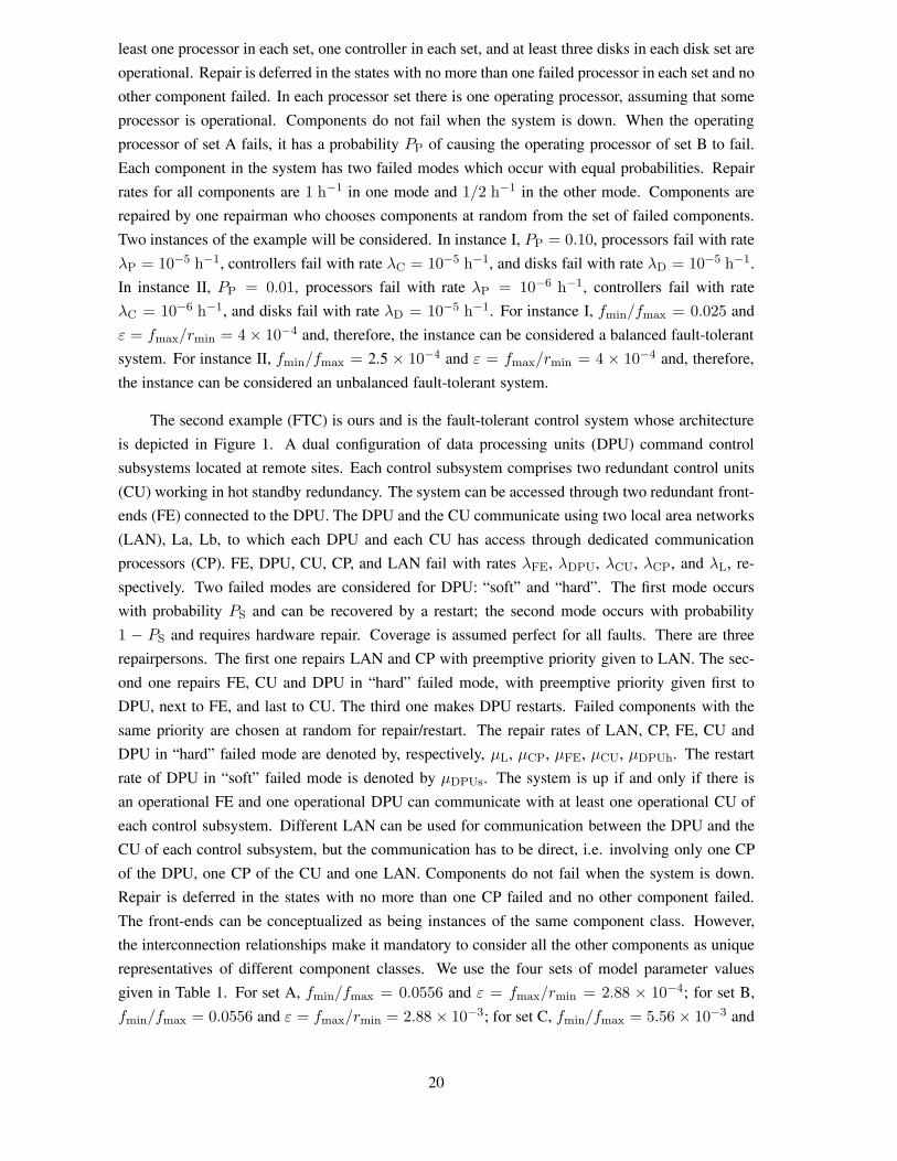
The second example (FTC) is ours and is the fault-tolerant control system whose architecture
is depicted in Figure 1. A dual configuration of data processing units (DPU) command control
subsystems located at remote sites. Each control subsystem comprises two redundant control units
(CU) working in hot standby redundancy. The system can be accessed through two redundant front-
ends (FE) connected to the DPU. The DPU and the CU communicate using two local area networks
(LAN), La, Lb, to which each DPU and each CU has access through dedicated communication
processors (CP). FE, DPU, CU, CP, and LAN fail with rates λFE, λDPU, λCU, λCP, and λL, re-
spectively. Two failed modes are considered for DPU: “soft” and “hard”. The first mode occurs
with probability PS and can be recovered by a restart; the second mode occurs with probability
1 − PS and requires hardware repair. Coverage is assumed perfect for all faults. There are three
repairpersons. The first one repairs LAN and CP with preemptive priority given to LAN. The sec-
ond one repairs FE, CU and DPU in “hard” failed mode, with preemptive priority given first to
DPU, next to FE, and last to CU. The third one makes DPU restarts. Failed components with the
same priority are chosen at random for repair/restart. The repair rates of LAN, CP, FE, CU and
DPU in “hard” failed mode are denoted by, respectively, μL, μCP, μFE, μCU, μDPUh. The restart
rate of DPU in “soft” failed mode is denoted by μDPUs. The system is up if and only if there is
an operational FE and one operational DPU can communicate with at least one operational CU of
each control subsystem. Different LAN can be used for communication between the DPU and the
CU of each control subsystem, but the communication has to be direct, i.e. involving only one CP
of the DPU, one CP of the CU and one LAN. Components do not fail when the system is down.
Repair is deferred in the states with no more than one CP failed and no other component failed.
The front-ends can be conceptualized as being instances of the same component class. However,
the interconnection relationships make it mandatory to consider all the other components as unique
representatives of different component classes. We use the four sets of model parameter values
given in Table 1. For set A, fmin/fmax = 0.0556 and ε = fmax/rmin = 2.88 × 10⁻⁴; for set B,
fmin/fmax = 0.0556 and ε = fmax/rmin = 2.88 × 10⁻³; for set C, fmin/fmax = 5.56 × 10⁻³ and
20

FE
FEDPU1
DPU2
CP1a
CP1b
CP2a
CP2b
La
Lb
CU11 CU12 CU51 CU52. . .
CP11a
CP11b
CP12a
CP12b
CP51a
CP51b
CP52a
CP52b
Figure 1: Architecture of the fault-tolerant control system (FTC example).
Table 1: Sets of model parameter values for the FTC example.
set A B C D
λFE 2 × 10⁻⁶ 2 × 10⁻⁶ 2 × 10⁻⁶ 2 × 10⁻⁶
λDPU 10−5 10−5 2 × 10⁻⁵ 4 × 10⁻⁵
λCU 2 × 10⁻⁶ 2 × 10⁻⁶ 4 × 10⁻⁷ 4 × 10⁻⁷
λL 10−6 10−6 10−6 10−6
λCP 5 × 10⁻⁷ 5 × 10⁻⁷ 10−7 10−4
PS 0.9 0.9 0.9 0.9μFE 0.5 0.05 0.05 0.05
μDPUh 0.5 0.05 0.05 0.05μDPUs 4 0.4 0.4 0.4μCU 0.5 0.05 0.05 0.05μL 0.2 0.02 0.02 0.02μCP 0.5 0.05 0.05 0.05
ε = fmax/rmin = 5.76 × 10⁻³; for set D, fmin/fmax = 4 × 10⁻³ and ε = fmax/rmin = 5 × 10⁻³.
Thus, the fault-tolerant system can be considered balanced for sets A and B and unbalanced for sets
C and D. Furthermore, for set D, there are regenerative cycles outside Skminwith significant relative
contributions to EP {Z}, and, therefore, that set tests the behavior of AFTDB ABFTDB in a hard
scenario which defies the heuristic supporting those importance sampling schemes.
For the examples corresponding to balanced fault-tolerant systems we will compare the per-
formance of AFTDB with that of FB. For the examples corresponding to unbalanced fault-tolerant
systems we will compare the performance of ABFTDB with that of BFB. The simulation method
is run with a target 99% confidence interval of ±0.2% and a maximum number of regenerative cy-
cles max rc = 10,000,000. As initial value for FB in FB and BFB we take 0.5. As initial values
for FB and DB in AFTDB and ABFTDB we take 0.8. For the K parameter described in [6] we
took a value 1,000. All CPU times are measured on a workstation with a Sun-Blade-1000 proces-
sor. Table 2 summarizes the obtained results. We give the estimate, number of regenerative cycles
and CPU times under AFTDB (ABFTDB), and the slow down factor of FB (BFB) defined as the
ratio between the CPU times required under FB (BFB) and the CPU time required under AFTDB
(ABFTDB) to achieve a confidence interval of same relative halfwidth. When the target confidence
21

Table 2: Comparison of importance sampling schemes.
example estimate cycles CPU time in s slow down factor
FTD (I) 1.9634 × 10⁻⁸ ± 3.90 × 10⁻¹¹ 4,331,000 158.8 24.5
FTD (II) 1.6542 × 10⁻⁸ ± 3.30 × 10⁻¹¹ 4,430,000 216.0 13.6
FTC (A) 2.7550 × 10⁻¹⁰ ± 5.50 × 10⁻¹³ 7,032,000 4,295 66.1
FTC (B) 2.7569 × 10⁻⁸ ± 5.50 × 10⁻¹¹ 6,999,000 4,262 66.2
FTC (C) 1.9720 × 10⁻⁸ ± 4.32 × 10⁻¹¹ 10,001,000 8,652 48.3
FTC (D) 3.9010 × 10⁻⁷ ± 3.18 × 10⁻⁹ 10,008,000 11,397 235
interval is not achieved, we compute the slow down factor using estimates for the CPU times which
would be required to achieve it, based on the rule that CPU time is proportional to the inverse of the
square of the relative confidence interval halfwidth. The results show that for balanced fault-tolerant
systems AFTDB can speed up significantly FB and for unbalanced fault-tolerant systems ABFTDB
can speed up significantly BFB. Overall, simulation under the new importance sampling schemes
seems to be efficient making it possible to obtain highly accurate estimates in affordable CPU times.
6 Conclusions
We have proposed new importance sampling schemes for the efficient simulation of CTMC models
of fault-tolerant systems with deferred repair. The new schemes have been proved to be robust.
We have also proved that previously proposed importance sampling schemes, FB and BFB, are
robust for the considered class of CTMC models. The new importance sampling schemes have been
motivated theoretically for balanced fault-tolerant systems and, for those systems, are guaranteed to
be more efficient than FB and BFB. Numerical analysis using representative examples has shown
that the new importance sampling schemes can achieve significant speedups over FB and BFB for
both balanced systems and unbalanced systems. Using the new importance sampling schemes it is
possible to achieve highly accurate estimates in reasonable CPU times. Alternatively, under the new
importance sampling schemes, it is possible to obtain estimates of reasonable accuracy in very small
CPU times, opening the way to simulation based system optimization.
References
[1] C. Alexopoulos and B. C. Shultes, “The Balanced Likelihood Ratio Method for Estimating Performance
Measures of Highly Reliable Systems,” in Proc. Winter Simulation Conference, Piscataway, New Jersey,
1998.
[2] C. Alexopoulos and B. C. Shultes, “Estimating Reliability Measures for Highly-reliable Markov Sys-
tems, Using Balanced Likelihood Ratios,” IEEE Trans. on Reliability, vol. 50, no. 3, September 2001,
pp. 265-280.
22
[3] A. Berman and R. J. Plemmons, Nonnegative Matrices in the Mathematical Sciences, SIAM, 1994.
[4] J. A. Carrasco , “Failure Distance-based Simulation of Repairable Fault-Tolerant Systems,” in Computer
Performance Evaluation, Elsevier, 1992, pp. 351–365.
[5] J. A. Carrasco and V. Sune, “An Algorithm to Find Minimal Cuts of Coherent Fault Trees with Event
Classes Using a Decision Tree,” IEEE Trans. on Reliability, vol. 48, no. 1, March 1999, pp. 31–41.
[6] J. A. Carrasco, “Failure Transition Distance-Based Importance Sampling Schemes for the Simulation
of Repairable Fault-Tolerant Computer Systems,” May 2005, to appear in IEEE Trans. on Reliability.
[7] A. E. Conway and A. Goyal, “Monte Carlo Simulation of Computer Systems Availability/Reliability
Models,” in Proc. 17th IEEE Int. Symp. on Fault-Tolerant Computing, 1987, pp. 230–235.
[8] G. Dahlquist and A. Bjorck, Numerical Methods, Prentice-Hall, 1974.
[9] A. Goyal, P. Heidelberger and P. Shahabuddin, “Measure Specific Dynamic Importance Sampling for
Availability Simulations,” in Proc. 1987 Winter Simulation Conference, A. Thesen, H. Grant and W. D.
Kelton (eds.), 1987, pp. 351–357.
[10] A. Goyal, P. Shahabuddin, P. Heidelberger, V. F. Nicola, and P. W. Glynn, “A Unified Framework for
Simulating Markovian Models of Highly Dependable Systems,” IEEE Trans. on Computers, vol. 42,
no. 1, January 1992, pp. 36–51.
[11] J. M. Hammersley and D. C. Handscomb, Monte Carlo Methods, Metheun, 1964.
[12] A. Hordijk, D. L. Iglehart, and R. Schassberger, “Discrete Time Methods for Simulating Continuous
Time Markov Chains,” Advances in Applied Probability, vol. 8, 1976, pp. 772-788.
[13] S. Juneja and P. Shahabuddin, “Fast Simulation of Markov Chains with Small Transition Probabilities,”
Management Science, vol. 47, no. 4, April 2001, pp. 547–562.
[14] S. Juneja and P. Shahabuddin, “Splitting-Based Inportance-Sampling Algorithm for Fast Simulation of
Markov Reliability Models with General Repair-Policies,” IEEE Trans. on Reliability, vol. 50, no. 3,
September 2001, pp. 235–245.
[15] E. E. Lewis and F. Bohm, “Monte Carlo Simulation of Markov Unreliability Models,” Nuclear Engi-
neering and Design, vol. 77, 1984, pp. 49–62.
[16] M. K. Nakayama, “A Characterization of the Simple Failure Biasing Method for Simulations of Highly
Reliable Markovian Systems,” ACM Trans. on Modeling and Computer Simulation, vol. 4, 1994, pp.
52–88.
[17] M. K. Nakayama, “General Conditions for Bounded Relative Error in Simulations of Highly Reliable
Markovian Systems,” Advances in Applied Probability, vol. 28, 1996, pp. 687–727.
[18] A. Reibman and K. S. Trivedi, “Numerical Transient Analysis of Markov Models,” Computers and
Operations Research, vol. 15, 1988, pp. 19–36.
[19] P. Shahabuddin, V. F. Nicola, P. Heidelberger, A. Goyal, and P. W. Glynn, “Variance Reduction in Mean
Time to Failure Simulations,” in Proc. 1988 Winter Simulation Conference, M. Abrams, P. Haigh and J.
Comfort (eds.), 1988, pp. 491–499.
23

[20] P. Shahabuddin, Simulation and Analysis of Highly Reliable Systems, Ph. D. thesis, Stanford University,
1990.
[21] P. Shahabuddin, “Importance Sampling for the Simulation of Highly Reliable Markovian Systems,”
Management Science, vol. 40, no. 3, March 1994, pp. 333–352.
[22] M. R. Spiegel, Mathematical Handbooh of Formulas and Tables, McGraw-Hill, 1968.
[23] W. J. Stewart, Introduction to the Numerical Solution of Markov Chains, Princeton University Press,
1994.
[24] T. Zhuguo and E. E. Lewis, “Component Dependency Models in Markov Monte Carlo Simulation,”
Reliability Engineering, vol. 13, 1985, pp. 45–61.
24