3021

Korean J. Chem. Eng., 33(10), 3021-3028 (2016)DOI: 10.1007/s11814-016-0167-6

pISSN: 0256-1115eISSN: 1975-7220

INVITED REVIEW PAPER

†To whom correspondence should be addressed.E-mail: zzhong@seu.edu.cnCopyright by The Korean Institute of Chemical Engineers.

Simulation of large biomass pellets in fluidized bed by DEM-CFD

Lingli Zhu, Zhaoping Zhong†, Heng Wang, and Zeyu Wang

Key Laboratory of Energy Thermal Conversion and Control of Ministry of Education,School of Energy and Environment, Southeast University, Nanjing 210096, China

(Received 27 January 2016 • accepted 15 June 2016)

Abstract−An improved numerical model was proposed to solve the problem that the traditional DEM-CFD (Dis-crete element method-computational fluid dynamics) method was not suitable for the flow simulation of large parti-cles. In the improved model, the large particle was regarded as an agglomerate of many small fictitious spheres. Herein,the drag force between gas and large pellets was assumed as a combined effect of that between gas and fictitiousspheres by volume penalty method. Based on the proposed model, the flow of the mixtures of large biomass pellets andquartz sands in fluidized bed was simulated. It shows that the existence of the biomass pellets has a great impact on theflow field. The flow patterns and pressure drops under different working conditions in simulation results have a goodagreement with that in experimental results partially, which also tests the proposed model.

Keywords: Multi-phase Systems, Computational Fluid Dynamics, Fluidization, Fluid-particle Dynamics

INTRODUCTION

Due to the energy shortage and stringent emission standards,more and more researchers are trying to discover alternative fuelsto substitute for fossil fuel. Biomass pyrolysis technology, which isone of the effective approaches to produce clean liquid fuel withhigh thermal value, has aroused a worldwide concern. The fluid-ized bed, comparing with many other reactors, has been widelyapplied to biomass pyrolysis for high reaction efficiency [1-3]. How-ever, the mixing of fluidizing agents and biomass particles, such assawdust and rice hull, was not very efficient in the previous re-searches [4,5]. In which, the layer phenomenon can be easily ob-served mainly due to the distinct density differences between thesetwo kinds of materials. To solve these problems, compression mold-ing technology is used here to increase the biomass particle den-sity from 600-700 kg/m3 to 1,300-1,400 kg/m3. In the present study,the discrete particle simulation of the mixtures consisting of quartzsands and compressed biomass pellets in fluidized bed has beencarried out, and authors hope that the successful flow simulationcan lay the foundation for pyrolysis or gasification simulation influidized bed.

DEM-CFD (Discrete element method - computational fluiddynamics) coupled method, first developed by Tsuji et al. [6], wasused to simulate the gas-solid flow in fluidized bed. In the DEM-CFD coupling method, the gas movement is governed by the tra-ditional continuity equation and Navier-Stokes equations, whileparticle-wall and particle-particle contact force is determined byDEM models [7]. The momentum exchange between gas and solidphase is usually expressed by Ergun [8] and Wen and Yu correla-tions [9] in mesoscale. With the advantage that the Eulerian ap-proach is able to trace the trajectory of each particle in the simula-

tion process, the DEM-CFD method has been widely used in thesimulation of dense gas-solid flow, such as bubbling fluidized bed,spouted bed and rotating fluidized bed [10-12]. In the present study,we applied the DEM-CFD coupling method to simulate the flowof the mixtures consisting of quartz sands and compressed bio-mass pellets in a fluidized bed. Considering the simulation accu-racy, the grid size in DEM-CFD should be not only large enoughfor the particle size, but also small enough for mesoscopic struc-tures such as bubbles, which limits the application of traditionalDEM-CFD coupling method to the simulation of the mixture oflarge particles and quartz sands (the size of compressed biomass par-ticles is usually larger than 10 mm, while the fluidized agent diam-eter is less than 1 mm). Inspired by the volume penalty method [13],where the large biomass particle is estimated by assuming that cyl-inder-shaped particles consisting of small fictitious spheres, theDEM-CFD method is improved and tested in this work.

In this paper, the improved DEM-CFD method for large cylin-der-shaped biomass particles was first introduced and then testedby the subsequent numerical simulation of gas flow around a fixedcylinder-shaped particle in a vertical channel. The proposed modelwas finally implemented in the simulation of the flow of biomassparticles and quartz sands.1. Improved DEM-CFD Model for Large Cylinder-shaped Parti-cles1-1. Discrete Element Method

The DEM method was proposed by Cundall and Strack, wherethe collision between particles was modeled by springs, dashpotsand sliders. Contacting force in DEM is divided into normal forcefcn and tangential force fct, which can be calculated by Eqs. (1) and(2) respectively.

fcn=−kndn−ηnvn (1)

fct=−kndt−ηtvt (2)

where, dn and dt represent the particle displacement in the nor-

3022 L. Zhu et al.

October, 2016

mal direction and tangential direction, respectively, vn and vt arethe particle relative velocity in the normal direction and tangentialdirection respectively, k is the spring stiffness, and η is the coeffi-cient of viscous dissipation. If |fct|>μf|fcn| is satisfied, fct should becalculated by Eq. (3).

fct=−μf|fcn|t (3)

where, μf is the coefficient of friction. The coefficient of viscous dis-sipation, η, can be calculated by the following correlations [14]:

η=2γ(mk)0.5 (4)

γ=α/(1+α2)0.5 (5)

α=−(1/π)lne (6)

where, e is the restitution coefficient of spring.Traditional DEM is not suitable for cylinder-shaped particles,

which was discussed above. Hence, the cylinder particle will beassumed as an agglomeration of fictitious spheres in section 1-3.1-2. CFD Model

Fluid motion is governed by the incompressible continuity andmomentum equations.

(7)

(8)

where, ε, u and p represent void fraction, locally averaged gas veloc-ity and gas phase pressure in a computational cell, respectively; ρf

is the gas density, and ν is gas kinematic viscosity.Gas-solid interaction force, f, is given by Eq. (9).

(9)

where, is the volume-weighted velocity of all solids in a compu-tational cell, which is defined by Eq. (10).

(10)

where, Np and Nfic represent the number of particles and fictitiousspheres in a computational cell, respectively, Vp and Vfic are the vol-ume of particle and fictitious sphere respectively, and arethe average velocity of particles and fictitious spheres in a cell re-spectively.

The drag coefficient, β, is given by Ergun correlation (ε≤0.8)and Wen & Yu correlation (ε>0.8) [15].

(11)

(12)

where, is the Reynolds number defined by Eq. (13).

(13)

where, is Sauter mean diameter in a computational cell, whichcan be obtained by Eq. (14).

(14)

where, αp and αc represent the volume fraction of particle and cyl-inder in a computational cell, respectively, and αfic is the volumefraction inside of a cylinder. dp and dfic are the particle diameter andfictitious sphere diameter, respectively.

The fluid force acting on particle, fp, and on cylinder, fc, can bedetermined by Eqs. (15) and (16).

(15)

(16)

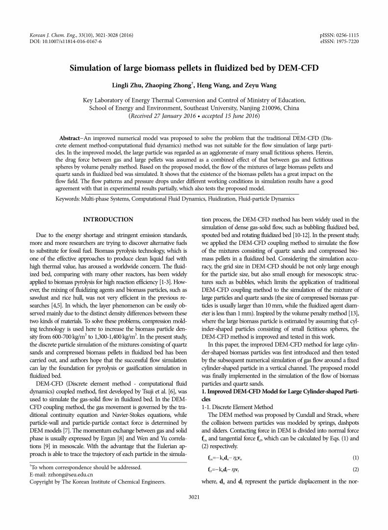
1-3. Testing of the Improved ModelTo test the improved model, the gas flow around a cylinder-

shaped particle fixed in the vertical channel is simulated. The geom-etry of the computational region is shown in Fig. 1(a) (the direc-tion of gas velocity is +z). The grid size is 2.5×dfic in simulation.The arrangement of fictitious particles is shown in Fig. 1(b). Thecylinder-shaped biomass particle, both length and diameter of whichare 10 mm, is regarded as an aggregation of 2072 fictitious sphereswith 0.8 mm (αfic=0.7). CD is given by Eq. (17).

(17)

∂ ε( )∂t---------- + ∇ εu( ) = 0•

∂ εu( )∂t

------------- + ∇ εuu( ) = − ε

ρf----∇p + εv∇2u + f•

f = β

ρf---- U − u( )

U

U = NPVPUP + NficVficUfic

NPVP + NficVfic-------------------------------------------------

UP Ufic

β =

μf 1− ε( )

d2ε

------------------ 150 1− ε( ) +1.75Re[ ] ε 0.8≤

34--CD

μf 1− ε( )

d2ε

------------------ε−2.7Re ε 0.8>

⎩⎪⎪⎨⎪⎪⎧ ~

~

CD = 24 1+ 0.15Re0.687( )/Re Re 1000≤0.43 Re 1000>⎩

⎨⎧ ~ ~ ~

~

Re~

Re = U − uρfεd

μf------------------------

~

d

d = 1− ε

αp

dp----- +

αcαfic

dfic-------------

------------------------

fp = βVP u − Upi( )

1− ε------------------------------ − ∇pVP

fc = αficβ u − Usj( )

1− ε---------------------- − ∇p⎝ ⎠⎛ ⎞dVcylinder∫

CD = 2fc

ρfAprojur2

--------------------

Fig. 1. Geometry of computational region and aggregation of ficti-tious spheres.

Simulation of large biomass pellets in fluidized bed by DEM-CFD 3023

Korean J. Chem. Eng.(Vol. 33, No. 10)

where, ur is the relative velocity between gas and particle. Aproj isthe projected surface area of the particle normal to the direction ofthe relative velocity between the particle and the local gas.

Aproj=A0 cosθ (18)

where, A0 is the maximum cross-sectional area of the cylinder-shaped particle, and θ is the inclination angle, which is also shownin Fig. 1.

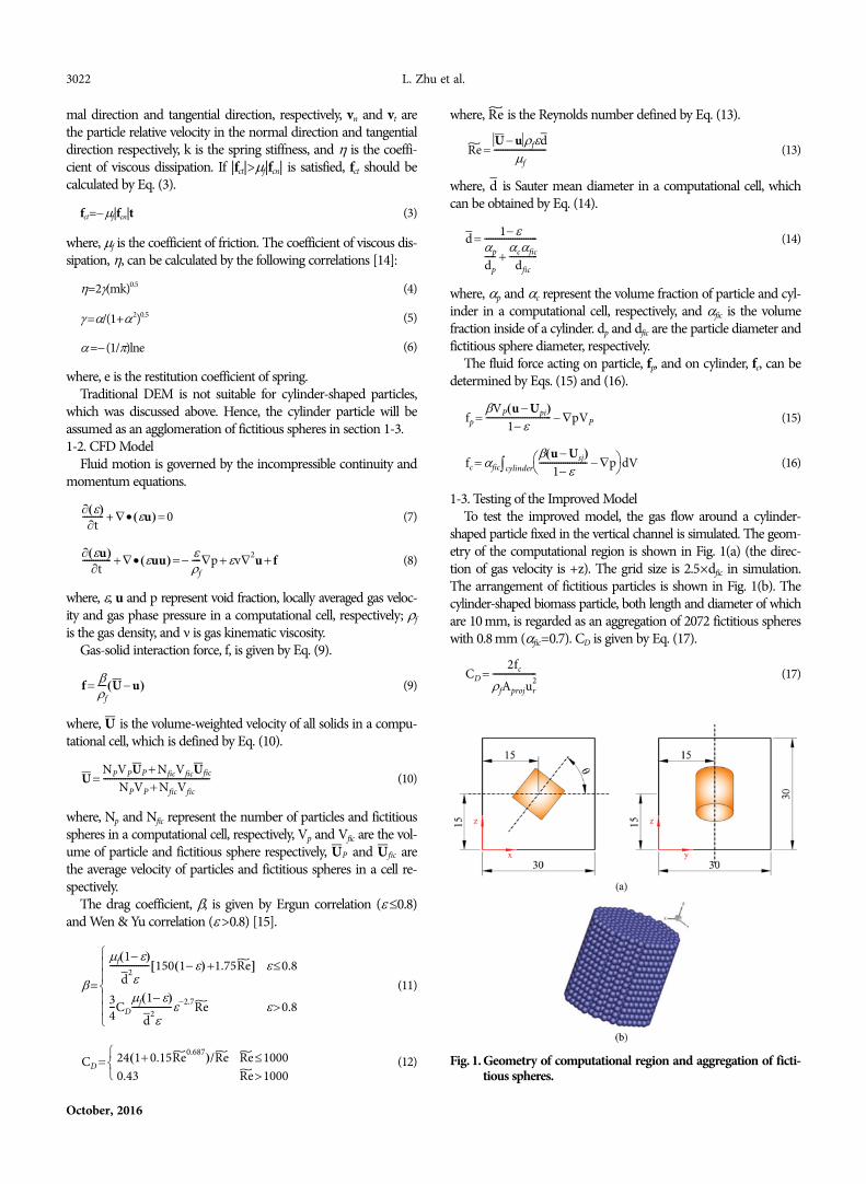
CD values under different Reynolds number and incline anglesin simulation are plotted by red line in Fig. 2, while CD calculatedby Eq. (19) [16-18] is depicted by the black line. It is found that CD

value decreases as Reynolds number, Re, increases. As Re<2000,CD decreases with the increase of Re sharply. However, the decreas-ing tendency becomes very flat when Re>4000. When Reynoldsnumber is low (Re<2000), CD value in simulation is less than thatcalculated by Eq. (19). However, CD value in simulation becomesmuch larger when Re>4000.

(19)CD = 24

ReP-------- 1+ C1ReP

C2( ) + C3

1+ C4/ReP( )----------------------------

Fig. 2. Comparison of CD value in simulation with that calculatedby empirical correlation.

Fig. 3. The schematic of domain decomposition method.

(20)

2. Simulation and Experimental SystemThe arrangement of fictitious particles in CFD part is the same

as that in the testing part. To form a cylinder in DEM part, 768spheres with the diameter of 3 mm are used to reduce the timespent in the collision calculation. The quartz sands have an aver-age diameter of 0.8 mm, and function as fluidizing agents. Thesolution methodology used for DEM-CFD simulation includesthe finite volume method (FVM), staggered grid method, semi-implicit method for pressure linked equations (SIMPLE), and thefirst-order upwind algorithm used for the DEM-CFD iterative pro-cess. To reduce the computation time, the computation domain isdivided into several sub-domains for parallel computation inspiredby the domain decomposition method [19], the scheme of which isshown in Fig. 3. Then computation tasks of different sub-domainsare assigned to different CPUs, exchanging the boundary informa-tion every calculation step by message passing interface (MPI)command. In the present studies, 12 threads in PC clusters are usedfor parallel computation at the same time. Other parameters in simu-lation are shown in Table 1, which are corresponding to the exper-iment.

The simulated inlet boundary conditions are shown in Fig. 4.The velocity inlet boundary condition is set for the square holesand the no-slip boundary condition is set for the others. The con-ventional pressure outlet boundary condition is chosen for the out-let boundary. All the mesh size in the direction of x, y, and z is2 mm. The superficial gas velocity is 1.5 m/s in both the experi-ment and simulation. So the inlet gas velocity of each discrete holein the distributor is 19.6 m/s.

C1= 0.0005ρp − ρf

ρf--------------

⎝ ⎠⎛ ⎞

1.1687ϕ

4.7677 da

dV-----

⎝ ⎠⎛ ⎞

6.5032

C2 = 0.6813ρp − ρf

ρf--------------

⎝ ⎠⎛ ⎞

−0.0534ϕ−1.0632 da

dV-----

⎝ ⎠⎛ ⎞

−1.5334

C3 = 0.6478ρp − ρf

ρf--------------

⎝ ⎠⎛ ⎞

−0.1328ϕ−3.8035 da

dV-----

⎝ ⎠⎛ ⎞

−3.3911

C4 = 22.4748ρp − ρf

ρf--------------

⎝ ⎠⎛ ⎞

−1.764ϕ−1.1738 da

dV-----

⎝ ⎠⎛ ⎞

5.1868

⎩⎪⎪⎪⎪⎪⎪⎨⎪⎪⎪⎪⎪⎪⎧

3024 L. Zhu et al.

October, 2016

The fluidization column as depicted in the detailed schematicof the experimental set-up (Fig. 5) is made of Plexiglas, the geom-etry of which is shown in Fig. 6. Fluidizing air supplied by aircompressor is measured by flowmeters to specify the gas velocityover the air distribution on the bottom. The flow regime of the

solid phase is shot by CCD camera with the frames per second(FPS) of 30, which is used to compare with the simulation result.To optimize the photo quality, a halogen lamp is used if needed.Pressure sampling system consists of pressure sensor, A/D con-verter and the terminal computer for collecting the pressure dropsignal.

Table 1. System parameters in simulationParameter Unit ValueQuartz sand diameter mm 0.8Quartz sand density kg/m3 2700Quartz sand number 420000Biomass particle size mm×mm 10×10Biomass particle density kg/m3 1350Grid size mm×mm×mm 2×2×2Biomass particle number 90Gas density kg/m3 1.205Gas kinematic viscosity m2/s 1.448×10−5

Time step of calculation s 1.5×10−5

Static bed height mm 80Restitution coefficient related to biomass particle 0.43Restitution coefficient related to sand particle 0.90Friction coefficient between particles 0.88Friction coefficient between particle and wall 0.77Spring stiffness in normal direction N/m 800Spring stiffness in tangential direction N/m 200

Fig. 4. The schematic of the velocity inlet boundary condition.

Fig. 5. The schematic of the experimental set-up.Fig. 6. Geometry of fluidization column.

Simulation of large biomass pellets in fluidized bed by DEM-CFD 3025

Korean J. Chem. Eng.(Vol. 33, No. 10)

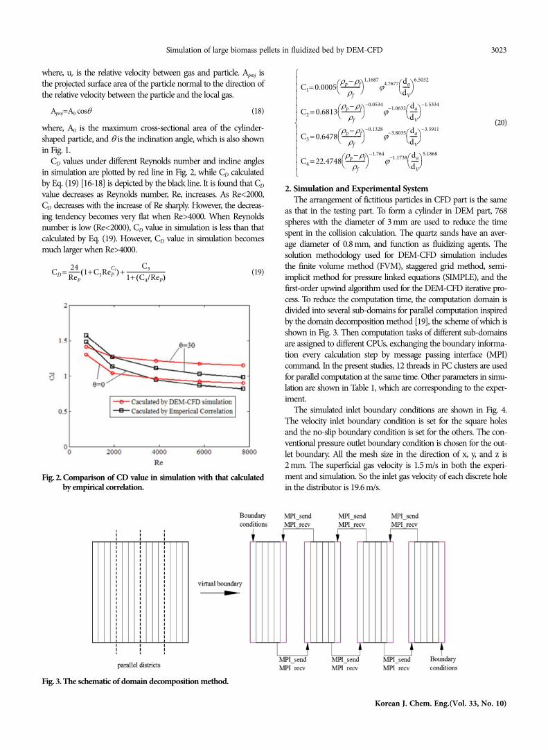
3. Simulation Results3-1. Snapshots of the Flow Pattern

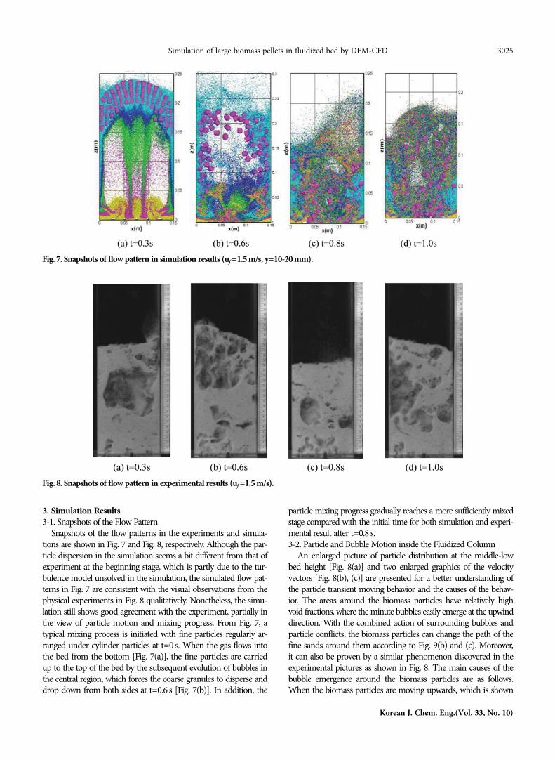
Snapshots of the flow patterns in the experiments and simula-tions are shown in Fig. 7 and Fig. 8, respectively. Although the par-ticle dispersion in the simulation seems a bit different from that ofexperiment at the beginning stage, which is partly due to the tur-bulence model unsolved in the simulation, the simulated flow pat-terns in Fig. 7 are consistent with the visual observations from thephysical experiments in Fig. 8 qualitatively. Nonetheless, the simu-lation still shows good agreement with the experiment, partially inthe view of particle motion and mixing progress. From Fig. 7, atypical mixing process is initiated with fine particles regularly ar-ranged under cylinder particles at t=0 s. When the gas flows intothe bed from the bottom [Fig. 7(a)], the fine particles are carriedup to the top of the bed by the subsequent evolution of bubbles inthe central region, which forces the coarse granules to disperse anddrop down from both sides at t=0.6 s [Fig. 7(b)]. In addition, the

particle mixing progress gradually reaches a more sufficiently mixedstage compared with the initial time for both simulation and experi-mental result after t=0.8 s.3-2. Particle and Bubble Motion inside the Fluidized Column

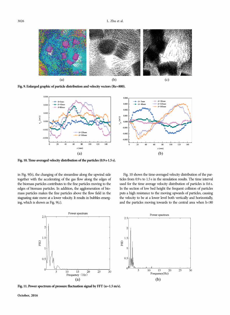
An enlarged picture of particle distribution at the middle-lowbed height [Fig. 8(a)] and two enlarged graphics of the velocityvectors [Fig. 8(b), (c)] are presented for a better understanding ofthe particle transient moving behavior and the causes of the behav-ior. The areas around the biomass particles have relatively highvoid fractions, where the minute bubbles easily emerge at the upwinddirection. With the combined action of surrounding bubbles andparticle conflicts, the biomass particles can change the path of thefine sands around them according to Fig. 9(b) and (c). Moreover,it can also be proven by a similar phenomenon discovered in theexperimental pictures as shown in Fig. 8. The main causes of thebubble emergence around the biomass particles are as follows.When the biomass particles are moving upwards, which is shown

Fig. 7. Snapshots of flow pattern in simulation results (uf =1.5 m/s, y=10-20 mm).

Fig. 8. Snapshots of flow pattern in experimental results (uf =1.5 m/s).

3026 L. Zhu et al.

October, 2016

in Fig. 9(b), the changing of the streamline along the upwind sidetogether with the accelerating of the gas flow along the edges ofthe biomass particles contributes to the fine particles moving to theedges of biomass particles. In addition, the agglomeration of bio-mass particles makes the fine particles above the flow field in thestagnating state move at a lower velocity. It results in bubbles emerg-ing, which is shown as Fig. 9(c).

Fig. 9. Enlarged graphic of particle distribution and velocity vectors (Re=800).

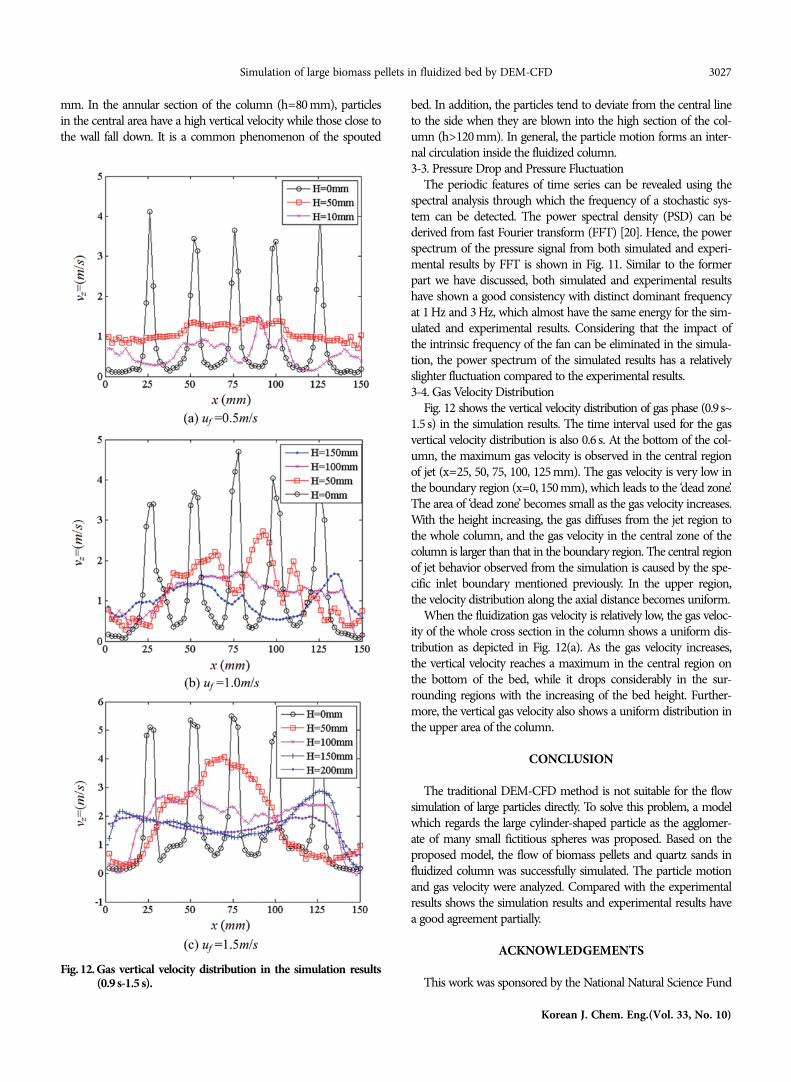
Fig. 10. Time-averaged velocity distribution of the particles (0.9 s-1.5 s).

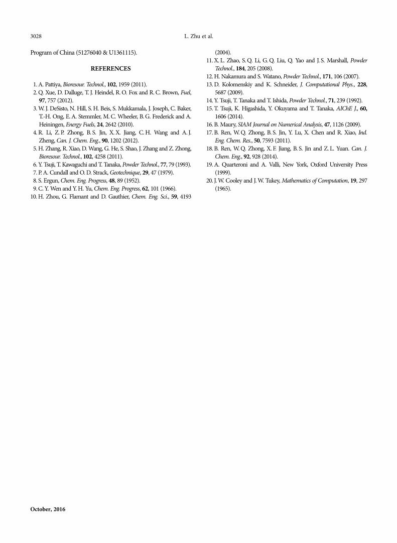
Fig. 11. Power spectrum of pressure fluctuation signal by FFT (u=1.5 m/s).

Fig. 10 shows the time-averaged velocity distribution of the par-ticles from 0.9 s to 1.5 s in the simulation results. The time intervalused for the time average velocity distribution of particles is 0.6 s.In the section of low bed height the frequent collision of particlesputs a high resistance to the moving upwards of particles, causingthe velocity to be at a lower level both vertically and horizontally,and the particles moving towards to the central area when h<80

Simulation of large biomass pellets in fluidized bed by DEM-CFD 3027

Korean J. Chem. Eng.(Vol. 33, No. 10)

mm. In the annular section of the column (h=80 mm), particlesin the central area have a high vertical velocity while those close tothe wall fall down. It is a common phenomenon of the spouted

bed. In addition, the particles tend to deviate from the central lineto the side when they are blown into the high section of the col-umn (h>120 mm). In general, the particle motion forms an inter-nal circulation inside the fluidized column.3-3. Pressure Drop and Pressure Fluctuation

The periodic features of time series can be revealed using thespectral analysis through which the frequency of a stochastic sys-tem can be detected. The power spectral density (PSD) can bederived from fast Fourier transform (FFT) [20]. Hence, the powerspectrum of the pressure signal from both simulated and experi-mental results by FFT is shown in Fig. 11. Similar to the formerpart we have discussed, both simulated and experimental resultshave shown a good consistency with distinct dominant frequencyat 1 Hz and 3 Hz, which almost have the same energy for the sim-ulated and experimental results. Considering that the impact ofthe intrinsic frequency of the fan can be eliminated in the simula-tion, the power spectrum of the simulated results has a relativelyslighter fluctuation compared to the experimental results.3-4. Gas Velocity Distribution

Fig. 12 shows the vertical velocity distribution of gas phase (0.9s~1.5 s) in the simulation results. The time interval used for the gasvertical velocity distribution is also 0.6 s. At the bottom of the col-umn, the maximum gas velocity is observed in the central regionof jet (x=25, 50, 75, 100, 125 mm). The gas velocity is very low inthe boundary region (x=0, 150 mm), which leads to the ‘dead zone’.The area of ‘dead zone’ becomes small as the gas velocity increases.With the height increasing, the gas diffuses from the jet region tothe whole column, and the gas velocity in the central zone of thecolumn is larger than that in the boundary region. The central regionof jet behavior observed from the simulation is caused by the spe-cific inlet boundary mentioned previously. In the upper region,the velocity distribution along the axial distance becomes uniform.

When the fluidization gas velocity is relatively low, the gas veloc-ity of the whole cross section in the column shows a uniform dis-tribution as depicted in Fig. 12(a). As the gas velocity increases,the vertical velocity reaches a maximum in the central region onthe bottom of the bed, while it drops considerably in the sur-rounding regions with the increasing of the bed height. Further-more, the vertical gas velocity also shows a uniform distribution inthe upper area of the column.

CONCLUSION

The traditional DEM-CFD method is not suitable for the flowsimulation of large particles directly. To solve this problem, a modelwhich regards the large cylinder-shaped particle as the agglomer-ate of many small fictitious spheres was proposed. Based on theproposed model, the flow of biomass pellets and quartz sands influidized column was successfully simulated. The particle motionand gas velocity were analyzed. Compared with the experimentalresults shows the simulation results and experimental results havea good agreement partially.

ACKNOWLEDGEMENTS

This work was sponsored by the National Natural Science FundFig. 12. Gas vertical velocity distribution in the simulation results

(0.9 s-1.5 s).

3028 L. Zhu et al.

October, 2016

Program of China (51276040 & U1361115).

REFERENCES

1. A. Pattiya, Bioresour. Technol., 102, 1959 (2011).2. Q. Xue, D. Dalluge, T. J. Heindel, R. O. Fox and R. C. Brown, Fuel,

97, 757 (2012).3. W. J. DeSisto, N. Hill, S. H. Beis, S. Mukkamala, J. Joseph, C. Baker,

T.-H. Ong, E. A. Stemmler, M. C. Wheeler, B. G. Frederick and A.Heiningen, Energy Fuels, 24, 2642 (2010).

4. R. Li, Z. P. Zhong, B. S. Jin, X. X. Jiang, C. H. Wang and A. J.Zheng, Can. J. Chem. Eng., 90, 1202 (2012).

5. H. Zhang, R. Xiao, D. Wang, G. He, S. Shao, J. Zhang and Z. Zhong,Bioresour. Technol., 102, 4258 (2011).

6. Y. Tsuji, T. Kawaguchi and T. Tanaka, Powder Technol., 77, 79 (1993).7. P. A. Cundall and O. D. Strack, Geotechnique, 29, 47 (1979).8. S. Ergun, Chem. Eng. Progress, 48, 89 (1952).9. C. Y. Wen and Y. H. Yu, Chem. Eng. Progress, 62, 101 (1966).

10. H. Zhou, G. Flamant and D. Gauthier, Chem. Eng. Sci., 59, 4193

(2004).11. X. L. Zhao, S. Q. Li, G. Q. Liu, Q. Yao and J. S. Marshall, Powder

Technol., 184, 205 (2008).12. H. Nakamura and S. Watano, Powder Technol., 171, 106 (2007).13. D. Kolomenskiy and K. Schneider, J. Computational Phys., 228,

5687 (2009).14. Y. Tsuji, T. Tanaka and T. Ishida, Powder Technol., 71, 239 (1992).15. T. Tsuji, K. Higashida, Y. Okuyama and T. Tanaka, AIChE J., 60,

1606 (2014).16. B. Maury, SIAM Journal on Numerical Analysis, 47, 1126 (2009).17. B. Ren, W. Q. Zhong, B. S. Jin, Y. Lu, X. Chen and R. Xiao, Ind.

Eng. Chem. Res., 50, 7593 (2011).18. B. Ren, W. Q. Zhong, X. F. Jiang, B. S. Jin and Z. L. Yuan. Can. J.

Chem. Eng., 92, 928 (2014).19. A. Quarteroni and A. Valli, New York, Oxford University Press

(1999). 20. J. W. Cooley and J. W. Tukey, Mathematics of Computation, 19, 297

(1965).