simulation of front instabilities in density-driven flow

Transp Porous Med (2016) 112:333–359DOI 10.1007/s11242-016-0649-3

Simulation of Front Instabilities in Density-Driven Flow,Using a Reactive Transport Model for BiogroutCombined with a Randomly Distributed PermeabilityField

W. K. van Wijngaarden1,2 · L. A. van Paassen3 ·F. J. Vermolen1 · G. A. M. van Meurs2 · C. Vuik1

Received: 24 July 2014 / Accepted: 9 February 2016 / Published online: 26 February 2016© The Author(s) 2016. This article is published with open access at Springerlink.com

Abstract Biogrout is a method to strengthen granular soil, which is based on microbial-induced carbonate precipitation. To model the Biogrout process, a reactive transport modelis used. Since high flow rates are undesirable for the Biogrout process, the model equationscan be solved with a standard Galerkin finite element method. The Biogrout process involvesthe injection of dense fluids in the subsurface. In this paper, we present our reactive transportmodel for Biogrout and use it to simulate an experiment in which a pulse of a dense fluidis injected in a porous medium filled with water. In this experiment, front instabilities wereobserved in the form of fingers. The numerical simulations showed that the fingering phe-nomenon was less pronounced than in the experiment. By reducing the dispersion length andimplementing a randomly distributed permeability field, the fingering phenomenon could beinduced. Furthermore, the results of a case study to a Biogrout application are reported.

Keywords Biogrout · Fingering · Randomly distributed permeability field · Microbial-induced carbonate precipitation (MICP) · Numerical simulation

List of symbols

x, y, z Cartesian coordinates (m)t Time (s)p Pressure (Pa)patm Atmospheric pressureq Darcy velocity (m/s)

B W. K. van [email protected]

1 Delft Institute of Applied Mathematics, Delft University of Technology,Mekelweg 4, 2628 CD Delft, The Netherlands

2 Unit Geo Engineering, Deltares, Boussinesqweg 1, 2629 HV Delft, The Netherlands

3 Delft University of Technology, Geoscience and Engineering, Stevinweg 1,2628 CN Delft, The Netherlands

123

http://crossmark.crossref.org/dialog/?doi=10.1007/s11242-016-0649-3&domain=pdf

334 W. K. van Wijngaarden et al.

v Pore water flow velocity (m/s)K Constant in the differential equation for the flow (m3/kmol)1 − Vs Liquid volume that disappears per number of converted particles (m3/kmol)k Intrinsic permeability (m2)dm Mean particle size of the grains (m)μ Dynamic viscosity of the fluid (Pa s)ρl Density of the fluid (kg/m3)mCaCO3 Molecular mass of calcium carbonate (kg/kmol)ρCaCO3 Density of calcium carbonate (kg/m3)g Gravitational constant (m/s2)θ Porosity (1)dm Mean particle size of the grains (m)M Mean of the log-normal distribution logN (μ̃, σ 2) that is used to model the

porosity (1)V Mean of the log-normal distribution logN (μ̃, σ 2) that is used to model the

porosity (1)CNa+

Concentration of sodium and chloride ions (kmol/m3)Curea Concentration of dissolved urea molecules (kmol/m3)CCa2+ Concentration of dissolved calcium ions (kmol/m3)CNH+

4 Concentration of dissolved ammonium ions (kmol/m3)CCaCO3 Concentration of calcium carbonate molecules (kg/m3)Sbac Ratio of the microorganisms that is fixated (with respect to the injected con-

centration) (1)D Dispersion tensor (m2/s)Dm Molecular diffusion coefficient (m2/s)αL Longitudinal dispersivity (m)αT Transverse dispersivity (m)rhp Reaction rate of the hydrolysis and precipitation processes (kmol/m3/s)vmax Maximal reaction rate (kmol/m3/s)Km,urea Saturation constant of urea (kmol/m3)

1 Introduction

The current research is done within the framework of Biogrout. It is investigated what theeffects of buoyancy-driven flow and the associated fingering phenomenon can be onBiogrout.

Biogrout is a soil strengthening method, which is based on microbial-induced carbon-ate precipitation (MICP). Microorganisms are used to produce the solid calcium carbonate(CaCO3), which strengthens the soil by connecting soil particles. The microorganisms arealready present in the soil (Paassen et al. 2010) or injected into it (Whiffin et al. 2007). Themicroorganisms are supplied with urea (CO(NH2)2) and calcium chloride (CaCl2). Thesesubstrates are injected into the soil and transported by water flow, induced by injection andextraction, to the desired location.Two reactions take place: a hydrolysis reaction and aprecip-itation reaction. The microbial enzyme urease provides the hydrolysis of urea, by which car-bonate (CO2−

3 ) is produced. The hydrolysis reaction equation is given inWhiffin et al. (2007):

CO(NH2)2 + 2H2Obacteria−→ 2NH+

4 + CO2−3 . (1)

In the presence of calcium ions (Ca2+), the carbonate precipitates as calcium carbonate(CaCO3):

123

Simulation of Front Instabilities in Density-Driven flow,. . . 335

Ca2+(aq) + CO2−3 (aq) → CaCO3(s). (2)

Combining both reaction (1) and reaction (2) gives the overall reaction equation:

CO(NH2)2(aq) + Ca2+(aq) + 2H2O(l) → 2NH+4 (aq) + CaCO3(s). (3)

The by-product of these reactions is ammonium chloride (NH4Cl), which is dissolved inwater. As it is not desirable that the ammonium chloride stays in the soil, it should beremoved. Therefore, the injection of substrates is followed by groundwater injection andextraction to rinse the remaining by-product solution.

The substrates and by-product of the reactions are dissolved in water, which increasesthe fluid density. For example, a 1 molar calcium chloride/urea solution has a density of1.1 × 103 kg/m3. If all the calcium chloride and urea of a 1 molar solution react, one endsup with a 2 molar ammonium chloride solution, which has a density of 1.03 × 103 kg/m3.In a fresh groundwater environment, the dense fluid will move more easily downwards thanupwards as a result of density differences. The forces of gravity and buoyancy can generatefront instabilities in the form of fingers where a dense fluid is on top of a less dense fluid. Inorder to get the microorganisms and their substrates at the desired location and extract theby-product, it is important to examine the effect of fingering on the flow and transport. Thiswill help to decide which concentrations and what flow rate should be used and where theinjection and extraction wells should be positioned.

To examine the effect of buoyancy-driven flow and the associated fingering phenomenon,an experiment has beenperformed, inwhich a pulse of salinefluid is injected in a porousmediaflow cell, generating a two-dimensional flow field. The flow cell is filled with glass beadsand saturated with water. The saline pulse is followed by a pulse of water. The experimentalresults are compared with the outcome of numerical simulations. Besides, a Biogrout casestudy is performed and reported.

A lot of research on fingering has already been done, both on viscous fingering (Saffman–Taylor instabilities) and instabilities caused by density differences; see, for example, Dierschand Kolditz (2002), Duijn et al. (2004), Farajzadeh et al. (2013), and Khosrokhavar et al.(2014). There are several approaches. One is the sharp interface approach in which the fluidsare assumed to be immiscible (Chevalier et al. 2006; DiCarlo 2013). Another approach isthe miscible fluid approach. If chemical reactions play a role (like in the Biogrout case), themiscible fluid approach should be taken, since the concentration can have a whole range ofvalues and does not only have to be binary at the vicinity of a sharp interface; see, for example,de Wit (2004), Johannsen et al. (2006), Musuuza et al. (2009), Simmons et al. (2001), andVoss and Souza (1987).

The setup of the experiment and the case study is given in the Sects. 2 and 3. The reactivetransport model for Biogrout, derived in Wijngaarden et al. (2011) and van Wijngaardenet al. (2013), is presented in Sect. 4. Section 5 contains the numerical methods that are usedto solve the model equations, and Sect. 6 reports the results, including the effect of using arandom porosity/permeability field to induce the fingering. In Sect. 7, some conclusions anddiscussion can be found.

2 Materials and Methods

To evaluate the effect of a buoyancy-driven flow on the distribution of injected solutes, atwo-dimensional porous media flow cell experiment is performed. The flow cell constructed

123


Fig. 1 A picture of some glass beads (spheres) that are used in the buoyancy-driven flow experiment

0 0.1 0.2 0.3 0.4 0.5 0.6 0.7 0.8 0.90

0.1

0.2

0.3

0.4

x [m]

z [m

]

Γclosed

ΓoutΓin

Γout

Fig. 2 Setup of the experiment. Injection well is denoted by Γin and the extraction wells by Γout . The otherboundaries (Γclosed) are closed

from a PVC frame with plexiglass front and back plates is 95cm wide, 45cm high, and 3cmthick. The space is filledwith glass beads, with a grain size ranging up to 200µm.A picture ofsome glass beads is shown in Fig. 1. Beside glass beads, also some crystals can be seen. Thesecrystals result from the Biogrout experiment that is performed after the buoyancy-driven flowexperiment that is reported here. One injection well, a hollow steel tube, is installed at thecenter of the flow cell, and two extraction wells are installed at mid-height about 12cm fromthe side of the flow cell as shown in Fig. 2.

A solution of 0.5M sodium chloride (NaCl) is prepared to which a bit of red food dyepowder (Allura Red, E129) is added. The porous media flow cell is first filled with water andflushed for several hours. The flow rate at the injection and extraction wells is kept constant,where the injection flow rate is equal to the total extraction flow rate of about 300mL/h. Ata certain moment, the sodium chloride solution is injected for a period of 30min after whichtap water is injected again. The flow of the red sodium chloride solution is monitored usinga Canon G7 compact camera at 10min time-lapse intervals.

123


3 Case Study Setup

Since the scale of the experiment is quite small compared to practical applications, we alsodo a case study of an application of Biogrout, i.e., to create a cemented zone underneath alevee in order to prevent piping (Blauw et al. 2012, 2013). Piping is an important failuremechanism of levees in the Netherlands (van Beek et al. 2010). Piping starts with heaveand cracking of the soft soil top layer at the land side of the levee. The cracks in the topsoft soil layer allow for seepage via the permeable sand layer underneath the clay levee. Ifthe water level difference between river and land side is large enough, sand grains may betransported along with the water flow. This will create a pipe underneath the levee, whichbecomes wider and wider as the process proceeds. Finally, this will lead to failure of thelevee and to breakthrough.

One way of decreasing the risk of failure of the levee due to piping is to broaden the levee.This will decrease the pressure gradients in the sandy layer, which is the driving force forthe process. This, however, is expensive and not always possible, for example, because ofexisting buildings close to the levee.

In those cases, Biogrout can be used to decrease the risk of failure due to piping. As itfixates the sand grains, it will prevent the creation of pipes, or block the propagation of pipes.While the Biogrouted sand will only have a minor decrease in permeability, the seepagewater will flow through the fixated sand body. Hence, the water will not seek another wayand herewith the risk of pipe formation is reduced.

Figure 3 shows the cross section of the configuration for the case study. It shows thelevee and the desired location of the Biogrouted sand body. The blue arrows indicate theseepage. The Biogrouted sand and the top clay layer should be connected to prevent theformation of pipes in between. Therefore, the injection drain is located close to the top claylayer. The extraction drains are 2m below the injection, since the dense fluid will tend tomove downwards and since we assume that a Biogrouted sand body of 2m depth provides asufficient barrier for the pipes. The distance between the extraction drains is 2m. This casestudy can be modeled through a 2D simulation, because of the symmetry. For our domainof computation Ω , we choose a depth of 6m and a width of 4m. We assume that thesedimensions are large enough so that the numerical results are not affected by the location ofthe boundaries.

In the numerical simulation, the seepage is not taken into account. Therefore, we obtaina symmetrical situation. Because of this symmetry, we only calculate the part left to theinjection drain and mirror the results. We take the mathematical model as described in Sect.

Fig. 3 Configuration for the case study (cross section). The levee is shown as well as the desired location ofthe Biogrouted sand body. The location of the injection and extraction drains is indicated. The blue arrowsdisplay the seepage for a high water situation

123


4.2 and the configuration as in Fig. 3. We position the origin of the coordinate system abovethe red circle in this figure, i.e., on the symmetry axes, at the bottomof the clay layer. Then, thecoordinates of the centers of the extraction wells are (±1,−2.2). The radius of the extractiondrains is 0.1m. The injection is placed under the clay layer of the dike. As a simplification,we use a part of the symmetry axis as the inflow boundary, namely the line segment betweenz = −0.3 m and z = −0.1 m. Hence, a line segment is used as the injection boundary ratherthan a semicircle.

As a flow rate, we choose Qin = 0.5 m3 per day per running meter of the drain (for thewhole domain). For comparison, this is twice as much as the flow rate in the porous mediaflow cell experiment. To prevent that the dense fluid will sink away, we choose a largerextraction flow rate, that is, Qout = 2 m3 per day per running meter of the drain for boththe extraction drains. Since there are two extraction drains, the total extraction flow rate iseight times as large as the injection flow rate. The injection Darcy velocity qin is calculatedfrom the injection flow rate via qin = Qin/Ain, in which Ain is the surface of the injection.In the same way, we have that the extraction Darcy velocity qout equals qout = Qout/Aout.The Biogrout liquids are injected for 12 hours, followed by the injection of water to rinsethe soil. As the inflow concentration of urea and calcium, we choose cin = 0.5 kmol/ m3.Afterward, water is injected which implies that cin is given by cin = 0 kmol/ m3 for t > 12h.Since ammonium chloride is a reaction product, the injected concentration is equal to 0.

4 Mathematical Model

In this section, we describe the model equations that are used to simulate the experiment. Theinitial conditions and boundary conditions are given as well. This is done for the experimentas well as for the case study.

4.1 Model Equations, Initial and Boundary Conditions for the Simulation of theExperiment

In this subsection, we describe the mathematical model as well as the initial and boundaryconditions that are used to simulate the experiment. This model is based on the reactivetransport model for Biogrout as reported in Wijngaarden et al. (2011) and slightly adaptedfor this experiment.

We assume that the flow is incompressible and therefore divergence free. Hence, in thedomain Ω , we have for time t ≥ 0:

∇ · q = 0. (4)

Here, q (m/s) is the Darcy flow velocity.For the relation between the Darcy flow velocity and the pressure, Darcy’s law is used

(Zheng and Bennett 1995):

q = − k

μ(∇ p + ρl gez), (5)

in which k (m2) is the intrinsic permeability, μ (Pa s) is the dynamic viscosity of the fluid, p(Pa) is the pressure, ρl (kg/m3) is the density of the fluid, and g (m/s2) is the gravitationalconstant.

123


The pore water velocity relates to the Darcy flow velocity via

v = qθ

, (6)

in which θ (1) is the porosity.Substituting Eq. (5) into Eq. (4) gives a partial differential equation for the pressure:

∇ ·(k

μ(∇ p + ρl gez)

)= 0, in Ω. (7)

This is the Oberbeck–Boussinesq approximation; see, for example, Diersch and Kolditz(2002). The Oberbeck–Boussinesq approximation consists in neglecting all density depen-dencies, except for the crucial buoyancy term ρl g in Eqs. (5) and (7).

We model the intrinsic permeability as a function of the porosity via the Kozeny–Carmanrelation (Bear 1972):

k = (dm)2

180

θ3

(1 − θ)2. (8)

In this equation, dm (m) is the mean particle size.We assume that the porosity is log-normallydistributed θ ∼ logN (μ̃, σ 2), see Kosugi (1996) and Nimmo (2004).

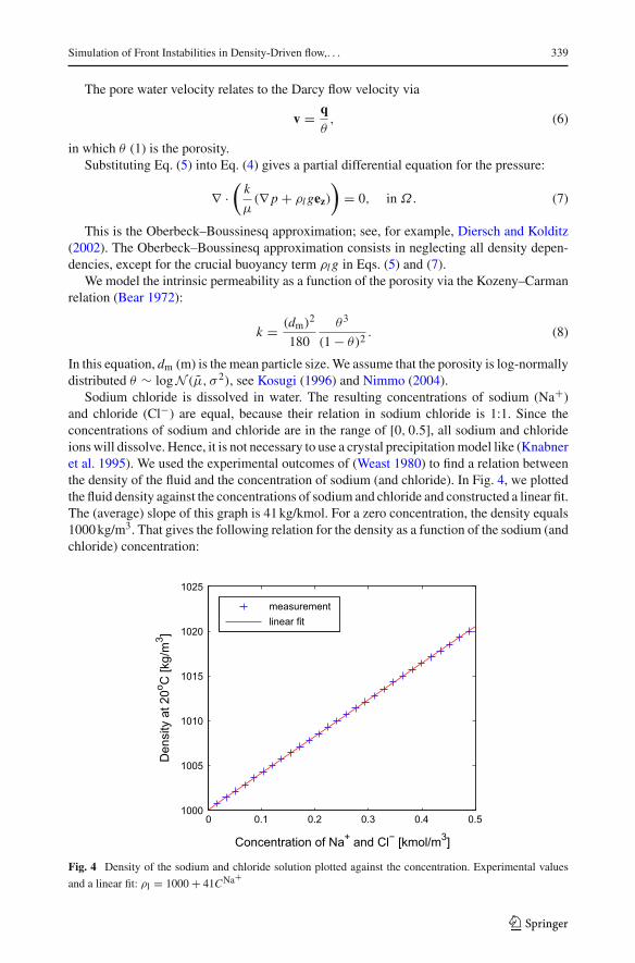
Sodium chloride is dissolved in water. The resulting concentrations of sodium (Na+)and chloride (Cl−) are equal, because their relation in sodium chloride is 1:1. Since theconcentrations of sodium and chloride are in the range of [0, 0.5], all sodium and chlorideionswill dissolve. Hence, it is not necessary to use a crystal precipitationmodel like (Knabneret al. 1995). We used the experimental outcomes of (Weast 1980) to find a relation betweenthe density of the fluid and the concentration of sodium (and chloride). In Fig. 4, we plottedthe fluid density against the concentrations of sodium and chloride and constructed a linear fit.The (average) slope of this graph is 41kg/kmol. For a zero concentration, the density equals1000kg/m3. That gives the following relation for the density as a function of the sodium (andchloride) concentration:

0 0.1 0.2 0.3 0.4 0.51000

1005

1010

1015

1020

1025

Concentration of Na+ and Cl− [kmol/m3]

Den

sity

at 2

0o C [k

g/m

3 ]

measurementlinear fit

Fig. 4 Density of the sodium and chloride solution plotted against the concentration. Experimental values

and a linear fit: ρl = 1000 + 41CNa+

123


ρl = 1000 + 41CNa+, (9)

in which CNa+(kmol/m3) is the concentration of sodium (which is equal to the chloride

concentration).The concentration of sodium is modeled by an advection–dispersion equation:

∂(θCNa+)∂t

= ∇(θD · ∇CNa+)

− ∇ · (qCNa+), in Ω. (10)

In this equation, D (m2/s) is the dispersion tensor, which coefficients equal Di j = (αL −αT)

viv j|v| + δi jαT

∑i

v2i|v| + δi j Dm, see Zheng and Bennett (1995). The constant αL (m) is the

longitudinal dispersivity, αT (m) is the transverse dispersivity, and Dm (m2/s) is themoleculardiffusion coefficient. In this study, we choose smaller values for αL and αT then given inGelhar et al. (1992), because the amount of dispersion is relatively small as indicated by thepresence of the fingers and the sharp fronts in the experiment. A large value for the entries inthe dispersion tensor would never show the observed fingering behavior. If dispersion wouldbemore important, then the dependence of the dispersion lengths on the statistical distributionof the permeability can be incorporated. Formore details andmathematical relations, we referto Talon et al. (2003, 2004).

We assume that the dispersion tensors for sodium and chloride are equal. Furthermore, itis assumed that the porous medium is not charged. Together with similar initial and boundaryconditions, we have that the sodium concentration and the chloride concentration are equal.Hence, we consider only one concentration, the sodium concentration. In this paper, wechoose the longitudinal dispersivity equal to the transverse dispersivity, αL = αT. Usually,the transverse dispersivity is somewhat smaller than the longitudinal dispersivity as reportedin Gelhar et al. (1992). We want the fronts as sharp as possible for the given mesh. A smallerdispersion length may lead to numerical instability, which is a result of the restriction onthe mesh Péclet number in case of central differences, see van Kan et al. (2005). Hence, wechoose equal dispersivities for this research.

The experiment is modeled in 2D with the configuration as shown in Fig. 2. The regionis denoted by Ω , which is bounded by Γclosed and by the holes Γin and Γout. The interfaceswith Ω and the injection and extraction wells are denoted by Γin and Γout, respectively.The diameter of the injection and extraction wells is 0.02m. The length of the domain isLx = 0.95m, and the height is Lz = 0.45m.

Initially, the pores are filled with tap water, and hence, we have that CNa+(t = 0, x) = 0

in Ω . In Table 1, the boundary conditions are given. Since the pressure should be prescribedsomewhere to get a unique solution for the pressure, we choose to prescribe the pressure atthe inflow. At the outflow boundaries, we prescribe the flow rate qout. The resulting injectionflow rate will be twice as large as the extraction flow rate. Of course, there is no flow over theclosed boundary. At the inflow boundary, we prescribe themass flux.We assume an advectiveflux at the outflow boundary, and there is no flux over the closed boundary.

Table 1 Boundary conditions for the concentration and the flow

Γin Γout Γclosed

CNa+ (θD∇C − qC) · n = 2qoutcin (θD∇C) · n = 0 (θD∇C − qC) · n = 0

q p = patm + ρl (x, z)g(Lz − z) q · n = qout q · n = 0

123


Fig. 5 Porosity in a region where fingers appear during the simulations. Left simulated porosity for theexperiment.Middle zoom in of left figure. Right simulated porosity for the case study. The porosity is shownfor a logN (0.42, 0.001) distribution

Table 2 Values that are taken forthe various constants dm = 200µm μ = 10−3 Pa s

Dm = 10−9 m2/s cin ={0.5 kmol/m3 0 ≤ t ≤ 0.5 h0 else

qout = M/18,000 m/s g = 9.81 m/s2

αL = 0.001 m αT = 0.001 m

patm = 105 Pa

We use a mesh with more than three hundred thousand elements. We assign a value forthe porosity to each element of this mesh. The values come from a log-normal distribution:θ ∼ logN (μ̃, σ 2). The mean M of this distribution equals M = eμ̃+σ 2/2, and the variance Vequals V = (eσ 2 − 1)e2μ̃+σ 2

. From the mean M and the variance V , one can calculate the μ̃

and σ 2 via μ̃ = log(

M2

V+M2

)and σ 2 = log

(V+M2

M2

). For each simulation, we use the same

sampling from the standard normal distribution for reasons of reproducibility. Subsequently,the resulting sample for each element is multiplied by the standard deviation of the normaldistribution, σ , and then shifted by the mean of this distribution, μ̃. Finally, the exponentialvalue is computed, which finally results into exp (μ̃ + σN (0, 1).) The variation in porosityis shown in the left two figures of Fig. 5 for a logN (0.42, 0.001) distribution.

We calculate the intrinsic permeability k with the Kozeny–Carman relation (8). Since thepermeability is a function of the porosity θ and the porosity varies from element to element,the permeability varies as well. The scale of variation for the chosen mesh is 1.1mm, whichis the square root of the total surface divided by the number of elements.

The values that have been assigned to the various constants are given in Table 2. The valueof qout has been chosen in such a way that the red area at time t = 0.5 h in the simulation hasthe same magnitude as in the experiment. As a result, the pore water velocities at the inflowboundary are equal for all the simulations of the experiment.

4.2 Model Equations, Initial and Boundary Conditions for the Case Study

In this case study, we try to create a cemented zone underneath a levee in order to preventpiping. Under the clay layer of the levee, the Biogrout substrates are injected for 12 hours,

123


followed by water injection to rinse the soil. Extraction drains are placed a few meters belowthe injection drain. In order to do this case study, we use the model for Biogrout as derivedin Wijngaarden et al. (2011) and van Wijngaarden et al. (2013). This model is based on thebiochemical reaction Eq. (3).

The concentrations of urea, calcium ions, and ammonium ions are modeled with theadvection–dispersion reaction equation:

∂(θCi )

∂t= ∇ · (θD∇Ci ) − ∇ · (qCi ) + miθrhp. (11)

In this equation, Ci is the concentration of species i , i ∈ {urea,Ca2+,NH+4 }, D is again

the dispersion tensor with coefficients as in Sect. 4.1, rhp is the rate of the overall Biogroutreaction (3), and mi is a constant that follows from the stoichiometry of the reaction. Asurea and calcium are consumed in the same ratio, their values of mi are equal and negative:murea = mCa2+ = −1. For the produced ammonium, we have mNH+

4= 2. The reaction rate

rhp is modeled with the following relation:

rhp = vmaxSbac Curea

Km,urea + Curea , (12)

in which vmax (kmol/m3/s) is the maximal microbial activity constant, Km,urea (kmol/m3) isthe saturation constant of urea and calcium chloride, and Sbac (1) is the ratio of microorgan-isms (with respect to the injected concentration) that is fixated in the placement procedureprior to the injection of the cementation fluids.

Since it is assumed that calcium carbonate is not transported, there is only a reaction termin the differential equation for the time derivative of its concentration:

∂CCaCO3

∂t= mCaCO3θrhp. (13)

In this equation, CCaCO3 is the concentration of calcium carbonate in mass per total volumerather than per liquid volume (kg/m3), and mCaCO3 (kg/kmol) is the molar mass of calciumcarbonate which is used to convert from kilomoles into kilograms.

As illustrated in Fig. 1, the calcium carbonate crystals are formed in the pores. Thiscauses a decrease in porosity where the increase in volume of calcium carbonate is equal tothe decrease in pore space. Hence, the following differential equation holds:

∂θ

∂t= − 1

ρCaCO3

∂CCaCO3

∂t, (14)

in which ρCaCO3 (kg/m3) is the density of calcium carbonate. In a homogenization procedure,

this equation is obtained if only one pore is considered. In Noorden (2009), a level setformulation is used to describe the crystal boundary for more complex geometries, and aformal homogenization procedure is applied to obtain upscaled equations. Equation (14) is acompromise between generality and complexity in the modeling. From the above differentialequation, the following relation between the porosity and the calcium carbonate content isderived:

θ(x, t) = θ(x, 0) − CCaCO3(x, t) − CCaCO3(x, 0)ρCaCO3

. (15)

Note that the above relation is an averaged approach compared to the upscaling approachesby Bringedal et al. (2015), Noorden (2009) and van Noorden et al. (2010).

123


For the flow, we also use the Oberbeck–Boussinesq approximation; see Eqs. (4)–(7).However, since the liquid volume decreases due to the reaction and since a solid (calciumcarbonate) is formed in the pore space, the right-hand side of Eq. (4) (and hence Eq. (7)) isnot equal to zero. Instead, we have:

∇ · q = K θrhp. (16)

The constant K (m3/kmol) has been defined as

K :=(mCaCO3

ρCaCO3

− (1 − Vs)

). (17)

As a result of the production of the solid calcium carbonate in the pores, there is less spaceavailable for the fluid. The decrease in pore space per unit of time ismCaCO3/ρCaCO3θrhp. Thisprocess is partly canceled since the hydrolysis and precipitation reactions cause a decrease inliquid volume. The decrease in liquid volume per kmol reacted urea/calcium chloride equals1 − Vs. For more details, we refer to van Wijngaarden et al. (2013). In the absence of thereaction (rhp = 0), this is again the Oberbeck–Boussinesq approximation. Substitution ofDarcy’s law (5) gives the following partial differential equation for the pressure:

∇ ·(

− k

μ(∇ p + ρl gez)

)= K θrhp. (18)

Again, we use the Kozeny–Carman relation (8) to model the intrinsic permeability as afunction of the porosity. The porosity is again log-normally distributed, with meanM = 0.42and variance V = 0.001. In the right plot of Fig. 5, a part of the porosity distribution in thedomain of computation is shown. In this case study, urea, calcium chloride, and ammoniumchloride are dissolved, rather that sodium chloride. Hence, the liquid density depends onthese species. As a relation between the liquid density ρl (kg/m3), and the urea concentration[Curea (kmol/m3)], the concentration of calcium ions [CCa2+ (kmol/m3)], and the ammoniumconcentration [CNH+

4 (kmol/m3)], we have:

ρl = 1000 + 15.4996Curea + 86.7338CCa2+ + 15.8991CNH+4 . (19)

The values that have been assigned to the various parameters are partly given in Table2. The used parameters that are not given in that table and the parameters that have anothervalue as in the simulation of the experiment are given in Table 3.

Table 3 Values that are taken forthe various constants in the casestudy

mCaCO3 = 100.1 kg/kmol 1 − VS = 0.02965m3/kmol

ρCaCO3 = 2710 kg/m3 vmax = 4.26 × 10−5 kmolurea/m3/s

Km,urea = 0.01 kmol/m3 Sbac = 0.25

Ain = 0.2 m Qin = 0.25m3/day/meter drain

Aout = 0.628 m Qout = 1.00m3/day/meter drain

qin = Qin/Ain qout = Qout/Aout

αL = 0.002 m cin ={0.5 kmol/m3 0 ≤ t ≤ 12 h0 else

αT = 0.002 m

123


Table 4 Boundary conditions for the case study

Boundary Concentration Flow

Symmetry boundary (qC − Dθ∇C) · n = 0 q · n = 0

Top boundary (“closed” clay layer) (qC − Dθ∇C) · n = 0 q · n = 0

Injection boundary Urea and calcium

(qC − Dθ∇C) · n = −qincin q · n = −qinAmmonium

(qC − Dθ∇C) · n = 0 q · n = −qinExtraction boundaries (Dθ∇C) · n = 0 q · n = qout

Right and bottom if q · n > 0 : (Dθ∇C) · n = 0 p = 2 · 105+Boundary (open) else: (qC − Dθ∇C) · n = 0 −ρl g(z − min(z))

We use a mesh with almost two million elements. Since the porosity varies from elementto element, the scale of variation (defined by the square root of the total surface divided bythe number of elements) is 2.5mm.

The boundary conditions for the flow and concentration in this case study are shown inTable 4. We have a no-flux condition on the top boundary and the symmetry boundary. At theinjection boundary, we prescribe the flow rate and the mass flux. At the extraction boundary,we also prescribe theflowrate, and since the concentration is unknownbeforehand,we assumean advective flux. At the bottom, right (and left) boundary, we assume hydrostatic pressure.We assume an advective flux in case of outflow over these boundaries and a zero mass flux incase of inflow, although we aimed at choosing the boundaries sufficiently far away such thatthe concentration at the boundary is (approximately) equal to zero. As an initial condition forthe aqueous concentrations, we take Curea = CCa2+ = CNH+

4 = 0 kmol/m3, for all points inthe domain of computation at time t = 0h. Initially, there is no calcium carbonate present inthe domain: CCaCO3 = 0 kg/m3, for all points in the domain of computation at time t = 0h. The partial differential equations for the concentrations of urea and calcium are equal(assuming that the dispersion coefficients are equal as well). Since the initial and boundaryconditions are also similar, these concentrations are equal. We will only show some resultsfor the urea concentration.

5 Numerical Methods

In this section, we explain which numerical methods are used to solve the partial differentialequations.

The partial differential equations are solved using the standard Galerkin finite elementmethod, with triangular elements and linear functions of local basis.

Since high flow rates are not desirable in the Biogrout process, the advection is notdominant and an upwind/stabilization method is not necessary. Since an upwind methoddecrease the order of convergence, in our case the Standard Galerkin method is a betterchoice.

Of course, also other, mass conserving, methods could have been applied like the mixedfinite element method (MFEM) or the finite volume (FV) method; see, for example, Kumaret al. (2013), Kumar et al. (2014), and Radu and Pop (2011), in which the convergence is

123


studied aswell. In Radu et al. (2013), themixed finite elementmethod is applied on a concretecarbonationmodelwith a variable porosity. Since the finite elementmethod is known to sufferfrompossible numericalmass conservation errors, we checkedmass conservation for the timeand mesh resolution that we used. We found numerically that the relative violation of themass balance was as small as a few tenths of a percent over the entire simulation.

In order to derive the weak formulation of the differential equations, the partial differentialequations are multiplied by a test function η and integrated over the domain Ω . For the timeintegration, an implicit Euler scheme is used.

The Newton–Cotes quadrature rules are used for the calculation of the element matricesand vectors. From these element matrices and vectors, the large matrices and vector arebuilt in MATLAB (R2013b_64). The MATLAB standard direct solver is used to solve thesubsequent systems. As a time step, we choose �t = 36s.

Most equations are coupled. We solve them decoupledly.In order to simulate the experiment, the various partial differential equations are solved,

and updates are done in the following order (in pseudocode):

1. ρn+1l : ρn+1

l = ρ(CNa+,n), according to Eq. (9);

2. pn+1 : ∇ ·(kμ(∇ pn+1 + ρn+1

l gez))

= 0, partial differential Eq. (7);

3. qn+1: qn+1 = − kμ(∇ pn+1 + ρn+1

l gez), partial differential Eq. (5);

4. CNa+,n+1:(θCNa+,n+1 − θCNa+, n

)/�t=∇·(θDn+1∇CNa+,n+1)−∇·(qn+1CNa+,n+1),

partial differential Eq. (10).

The following list presents in pseudocode the order in which the equations are solved andthe updates are done for the Biogrout case study:

1. ρn+1l : ρn+1

l = ρ(Curea,n,CCa2+,n,CNH+4 ,n), according to Eq. (19);

2. θn+1 : θn+1 = θ(θ0,CCaCO3,n), according to Eq. (15);3. kn+1 : kn+1 = k(θn+1), according to Eq. (8);

4. pn+1 : ∇ ·(kn+1

μ(∇ pn+1 + ρn+1

l gez))

= K θn+1rnhp, partial differential Eq. (18);

5. qn+1: qn+1 = − kn+1

μ(∇ pn+1 + ρn+1

l gez), partial differential equation (16);

6. Curea,n+1 : (θn+1Curea,n+1 − θnCurea,n

)/�t = ∇ · (θn+1Dn+1∇Curea,n+1) − ∇ ·

(qn+1Curea,n+1) − θrn+1hp , partial differential equation (11). Due to the reaction term,

this partial differential equation is nonlinear in the urea concentration. Newton’s methodis used to deal with that. In the Biogrout case, this method usually converges in threeiterations.

7. CNH+4 ,n+1:

(θn+1CNH+

4 ,n+1 − θnCNH+4 ,n+1

)/�t = ∇ · (θn+1Dn+1∇CNH+

4 ,n+1) −∇ · (qn+1CNH+

4 ,n+1) − θrn+1hp , partial differential equation (11). The values for rn+1

hpfollow from the last Newton iteration in the previous step;

8. CCaCO3,n+1:(CCaCO3,n+1 − CCaCO3,n

)/�t = mCaCO3θ

n+1rn+1hp , partial differential

equation (13).

We also investigated the effect of inner iterations on the results. This was done by recal-culating the density at each time step. If the difference between the previously calculateddensity was larger than some tolerance, the equations were solved with the updated densityuntil the difference was smaller than some tolerance. Convergence was usually reached inone or two iterations. Figure 6 shows some results for the scheme for Biogrout, proposedabove. The left plot of Fig. 6 shows the convergence behavior on a cross section for a two-dimensional Biogrout test case. In each refinement step, the time step size is divided by two

123


0 0.2 0.4 0.6 0.8 10

0.2

0.4

0.6

0.8

1

x[m]

urea

con

cent

ratio

n [k

mol

/m3]

refine1−with inner iterationsrefine4−with inner iterationsrefine1−without inner iterationsrefine4−without inner iterations

0 0.2 0.4 0.6 0.8 10

0.2

0.4

0.6

0.8

1

x[m]

urea

con

cent

ratio

n [k

mol

/m3]

refine1−without inner iterationsrefine2−without inner iterationsrefine3−without inner iterationsrefine4−without inner iterations

Fig. 6 Left Convergence of the Biogrout scheme without inner iterations. Right Scheme without inner itera-tions compared to the scheme with inner iterations

and the mesh size is divided by√2, since the expected order of convergence isO(h2 + �t),

with h a measure for the mesh size and �t the size of the time step. Figure 6 shows a niceconvergence behavior. In the right plot of this figure, the scheme without inner iterations iscompared to the scheme with inner iterations. This is done for the coarsest and the finestsimulation. It appears that the scheme with inner iterations only leads to small differencescompared to the scheme that was proposed here. When using small time steps, there were nonoticeable changes. Similar results were obtained for the other scheme, while investigatingthe effect of inner iterations on the results.

6 Results

6.1 Results of the Experiment and a Simulation with a Homogeneous PorousMedium

This section reports some results of the two-dimensional porous media flow cell experimentthat has been performed. The experimental results are compared to the results of a simulationusing a constant porosity and permeability. The left column of Fig. 7 shows some results ofthe flow cell experiment. The red fluid is the dense fluid. The color of the zones, where onlywater is present, ranges fromwhite to yellow, depending on the daylight and the artificial light.The colors in between this background color and the red color correspond to a concentrationbetween 0 and the injected concentration which is 0.5kmol/m3, but the exact relation is notknown. At t = 0.5h, the injection of the dense fluid stops and the injection of water starts.This gives the red ring in the pictures for t = 1h, t = 2h, t = 3h, t = 4h and t = 5h. Fromt = 2h, fingers appear on roughly two locations: on the bottom of the ring and on the topof the ring where the heavy fluid is above the less dense fluid. In either case, fingers appearon positions where a dense fluid is on top of a less dense fluid. Note that the fingers on thebottom of the ring are larger.

The right column of Fig. 7 shows some results of a simulation of this experiment, usinga porosity of θ = 0.42 and a permeability of k = 5.0 × 10−11 m2. As can be seen in thesimulation, no fingers appear. Apparently, the numerical noise is not sufficient to trigger thefingering. Hence, in the next section, we will vary the porosity and permeability to triggerthe fingering.

123


Fig. 7 Some pictures of the experiment (left) and the numerical simulation with a homogeneous porousmedium (right) at several times (from top to bottom t = 0.5h, t = 1h, t = 2h, t = 3h, t = 4h and t = 5h).In the simulation, the porosity θ equals θ = 0.42 and the intrinsic permeability k is k = 5.0 × 10−11 m2

123


6.2 Numerical Results for an Inhomogeneous Porous Medium

In this section, we use an inhomogeneous porosity within our simulations. We assign a valuefor the porosity to every element of themesh. The values come from a log-normal distribution:θ ∼ logN (μ̃, σ 2). We vary the mean porosity M and the variance V of this distribution anddo several simulations. As the mean M we choose: M = 0.36, M = 0.42, and M = 0.49.For the variance we choose: V = 0.0001, V = 0.001, and V = 0.005. This results in ninedifferent combinations. From the mean M and the variance V , one can calculate the μ̃ and

σ 2 via μ̃ = log(

M2

V+M2

)and σ 2 = log( V+M2

M2 ). The permeability that corresponds to a

mean porosity of M = 0.36 equals k = 2.5 × 10−11 m2, according to the Kozeny–Carmanrelation (8). The corresponding permeabilities of the means M = 0.42 and M = 0.49 arek = 5.0 × 10−11 m2 and k = 10 × 10−11 m2, respectively.

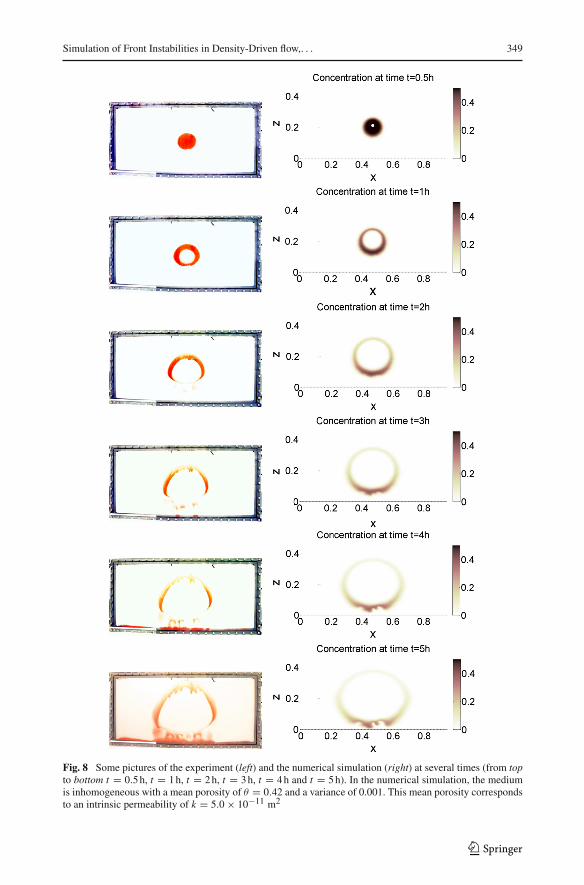
In the right column of Fig. 8, some results are shown for one of the simulations. In thissimulation, the mean porosity is M = 0.42 and the variance is V = 0.001. In the numericalsimulation with the homogeneous medium, of which the results are shown in Fig. 7, nofingers appear. In contrast to this simulation, we now see the same phenomenon as in theexperiment in Fig. 8. Moreover, fingers start to appear at approximately the same time as inthe experiment.

There are also some differences between modeling and the experiment. In the simulation,the fingers only appear on the bottom side of the ring, whereas in the experiment, also somesmall fingers appear at the bottom side of the top of the ring. Furthermore, the speed of thefingers in the experiment is larger than in the numerical simulation. From the results of theexperiment, it can be seen that the layer close to the lowest boundary is more permeable thanelsewhere. At time t = 4h, the red fluid reaches the bottom, and in one hour (at time t = 5h),it has already reached the left and right boundaries. Apparently, there is some space betweenthe frame and the plexiglass.

Figure 9 shows the effect of the value of the variance. Since the random number generatoris reset before every simulation, the values of the porosity are constructed from the same setof random numbers, as explained in Sect. 4. Hence, the fingers appear at the same location.The magnitude, however, depends on the value of the variance. A larger variance results inlonger fingers.

Figure 10 displays the effect of the variation in the meanM. Clearly, the value of the meanhas a large effect on the fingering phenomenon. For a small mean, hardly any fingers arise.A larger mean results in more fingers, and clearly, the bottom is reached earlier. The effectof the mean value of the porosity on the density effect is explained below. Remember thatthe pore water velocity at the inlet is kept constant in the simulations.

The pore water velocity is determined by combining Eqs. (5), (6) and (8):

vx = − (dm)2

180μ

θ2

(1 − θ)2

∂p

∂x, (20)

vz = − (dm)2

180μ

θ2

(1 − θ)2

∂p

∂z− (dm)2

180μ

θ2

(1 − θ)2ρl g. (21)

In case of a higher porosity, the term θ2

(1−θ)2is also larger. Now, remember that the pore water

velocity at the inlet is constant. Hence, the increase in the porosity term in the first term atthe right-hand side of Eqs. (20) and (21) is compensated by smaller pressure gradients inthese terms. Now, let the ratio between the buoyancy term and the pressure gradient term inthe right-hand side of Eq. (21) be a measure for the effect of the density differences. This

123


Fig. 8 Some pictures of the experiment (left) and the numerical simulation (right) at several times (from topto bottom t = 0.5h, t = 1h, t = 2h, t = 3h, t = 4h and t = 5h). In the numerical simulation, the mediumis inhomogeneous with a mean porosity of θ = 0.42 and a variance of 0.001. This mean porosity correspondsto an intrinsic permeability of k = 5.0 × 10−11 m2

123


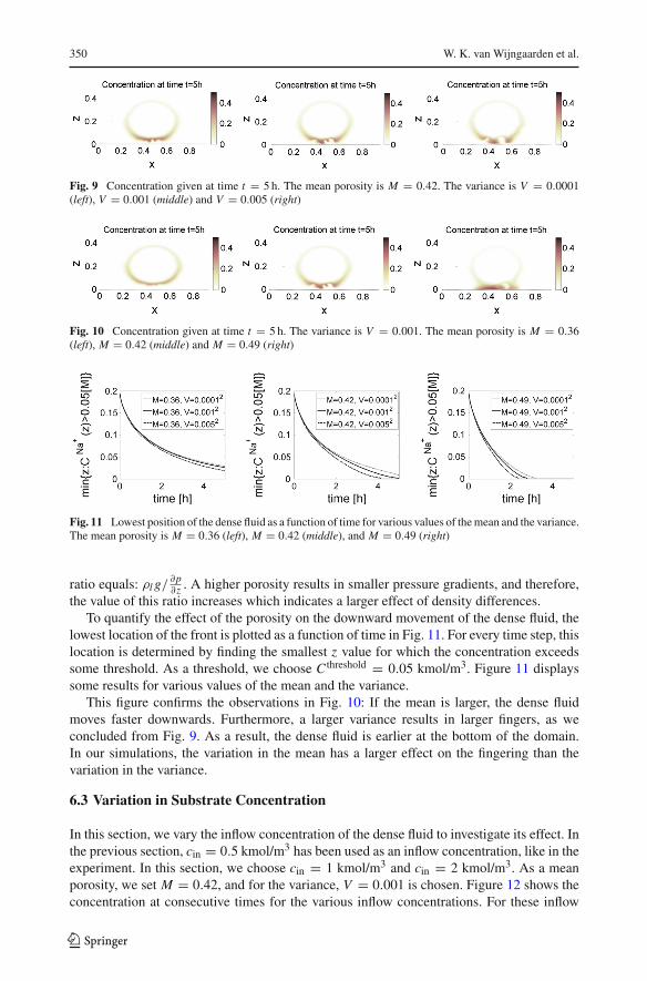
Fig. 9 Concentration given at time t = 5 h. The mean porosity is M = 0.42. The variance is V = 0.0001(left), V = 0.001 (middle) and V = 0.005 (right)

Fig. 10 Concentration given at time t = 5 h. The variance is V = 0.001. The mean porosity is M = 0.36(left), M = 0.42 (middle) and M = 0.49 (right)

Fig. 11 Lowest position of the dense fluid as a function of time for various values of themean and the variance.The mean porosity is M = 0.36 (left), M = 0.42 (middle), and M = 0.49 (right)

ratio equals: ρl g/∂p∂z . A higher porosity results in smaller pressure gradients, and therefore,

the value of this ratio increases which indicates a larger effect of density differences.To quantify the effect of the porosity on the downward movement of the dense fluid, the

lowest location of the front is plotted as a function of time in Fig. 11. For every time step, thislocation is determined by finding the smallest z value for which the concentration exceedssome threshold. As a threshold, we choose C threshold = 0.05 kmol/m3. Figure 11 displayssome results for various values of the mean and the variance.

This figure confirms the observations in Fig. 10: If the mean is larger, the dense fluidmoves faster downwards. Furthermore, a larger variance results in larger fingers, as weconcluded from Fig. 9. As a result, the dense fluid is earlier at the bottom of the domain.In our simulations, the variation in the mean has a larger effect on the fingering than thevariation in the variance.

6.3 Variation in Substrate Concentration

In this section, we vary the inflow concentration of the dense fluid to investigate its effect. Inthe previous section, cin = 0.5 kmol/m3 has been used as an inflow concentration, like in theexperiment. In this section, we choose cin = 1 kmol/m3 and cin = 2 kmol/m3. As a meanporosity, we set M = 0.42, and for the variance, V = 0.001 is chosen. Figure 12 shows theconcentration at consecutive times for the various inflow concentrations. For these inflow

123


Fig. 12 Concentration for an inflow concentration of cin = 1 kmol/m3 (left column) and cin = 2 kmol/m3

(right column) at several times (from top to bottom t = 0.5h, t = 1h, t = 2h, t = 3h, t = 4h and t = 5h).The mean porosity is M = 0.42, and the variance is V = 0.001

concentrations, the flow is considerably affected by the density differences. A higher inflowconcentration results into a heavier fluid. Therefore, the gravity component is larger, andhence, the dense fluid reaches the bottom earlier. Since the gravity component becomes more

123


significant for a higher inflow concentration, the pressure term is relatively less important,and this results into a buoyancy-dominated flow. Since the bottom is earlier reached, thereis less time for the formation of fingers. At the other hand, the density differences are larger,which is in favor of the formation of the fingers.

6.4 Case Study Simulations

In this section, we present the results of the case study simulations. We use the configuration,initial and boundary conditions as proposed in Sect. 4.2, combined with the heterogeneousporosity distribution. The aim was to construct a calcium carbonate wall as a barrier forthe pipes. In order to prevent waste of materials, it is desirable that the urea (and calcium)are consumed rather than extracted. Besides that, it is necessary to remove the ammoniumbecause of its impact on the environment.

6.4.1 Development of the Various Concentrations

Figure 13 shows how the concentrations of urea, calcium carbonate, and ammonium developin the domain of computation. The concentration profiles are shown at several times. After12 hours, the injection of the Biogrout substrates (in the top of the domain) was stoppedand the water injection started. This causes a region around the injection well with zero ureaconcentration, which is visible in the plot of the urea (and calcium) concentration at timet = 13h. The urea is forced downward by injection/extraction and by the density differences.At time t = 13h, the large urea plume just started splitting in two large fingers. We see thesame for the produced ammonium. In the right plot of Fig. 5, the initial porosity distributionis shown for this particular region.

At time t = 22h, in the same region small fingers arise, but also at the deepest locationof the urea and ammonium front. At time t = 25h, these small fingers are increased.

At time t = 45h, the urea and calcium are consumed, and the calcium carbonate wallhas his final shape. A barrier for the pipes has been formed. The plot of the ammoniumconcentration for this time shows thatmore andmore fingers arise. Due to density differences,these fingers tend to flow down. On the other hand, the extraction (indicated by the whitecircles) pulls them upward.

6.4.2 Extraction of Ammonium

In the left column of Fig. 14 is shown how the ammonium concentration evolves further intime. The heterogeneous porosity causes the ammonium plume to split into two parts (timet = 22 h) and later on in multiple fingers that are being extracted (times t = 60 h and t = 100h). On the symmetry axis x = 0, the horizontal fluid velocity caused by the extraction drainsis equal to zero, since the effect of one extraction well is canceled by the other. Closer to theextraction drain, the horizontal velocity in the direction of the drain increases. The splittingof the ammonium plume brings the ammonium closer to the extraction wells. After all theurea are consumed, the ammonium concentration decreases as a result of the extraction.Hence, the density difference with the surrounding water decreases, which makes it easierto extract the ammonium. After 100h, only 4 mol ammonium is left in the domain and 121mol ammonium was extracted.

123


Fig. 13 Results of the case study simulation with the heterogeneous porosity distribution for time t = 13 h,t = 22 h, t = 25 h and t = 45h. Presented are the urea concentration (left column), the calcium carbonateconcentration (middle column), and the ammonium concentration (right column)

123


6.4.3 Comparison with a Homogeneous Porosity Distribution

We repeated the same simulation for a homogeneous porosity. The ammonium concentrationat several times is shown for this simulation in the right column of Fig. 14. In this case,only one plume is observed and no fingers appear. The ammonium plume moves downwardsbetween the extraction wells. Although the flow rate of the extraction wells is eight times aslarge as the injection flow rate, only a part of the ammonium is extracted. After 100h, only50 mol is extracted, while 75 mol ammonium is still in the soil. In these simulations, theformation of fingers is advantageous for the removal of ammonium.

Figure 15 shows the distribution of the calcium carbonate for the simulation with theheterogeneous porosity distribution and the one with the homogeneous porosity. The aimwas to create a calcium carbonate wall below the clay layer of at least 2m length to decreasethe risk on piping. The top 2m of the calcium carbonate wall is similar for both simulations.Below these 2m, the distribution of calcium carbonate is rather different. The fingers in theurea and ammonium plume in the simulation with the heterogeneous porosity are also visiblein the calcium carbonate profile. Of course, this is not surprising, since calcium carbonatecan only be formed where urea is present. In the simulation with the heterogeneous porosity,6.22kg of calcium carbonate was formed in the soil. In the simulation with the homogeneousporosity, the amount of extracted urea was a little lower and the amount of produced calciumcarbonate was therefore a little higher: 6.25kg.

7 Discussion and Conclusions

In the experiment, fingers arise as expected where the dense fluid is on top of the less densefluid. This happens particularly at the bottom side of the ring. But also at the bottom side of thetop of the ring, small fingers come into being, which flow downwards, in opposite direction tothe flow that is generated by injection and extraction. In the simulation, no fingers appearedin case of a homogeneous medium. When using a variable porosity according to a log-normal distribution, fingers developed in the numerical simulation. Fingers started to appearat approximately the same time as in the experiment. Several simulations were performedfor various values of the mean porosity and variance. These simulations showed that a largevariation in porosity (and hence permeability) results in larger fingers than a small variation,but this effect is not very large. The variation in the mean porosity has a much larger effecton the fingers as shown in Fig. 10. The reason is explained in Sect. 6.2.

In comparison with the experiment, the numerical simulations seem to underestimatethe fingering phenomenon. Fingers only appear at the bottom side of the ring, while in theexperiment also some small fingers appear at the inside of the top of the ring. Furthermore,the flow velocity of the fingers in the experiment is larger than in the numerical simulations.

The numerical simulation, in which the inflow concentration was varied, showed that theconcentration has a large effect on the flow as shown in Fig. 12. Compared to the experimentand simulation with an inflow concentration of cin = 0.5 kmol/m3, the dense fluid movesdownward more rapidly for a higher value for the inflow concentration.

The case study simulations showed that the fingering phenomenon has not necessarily anegative effect on the extraction of the ammonium. By the formation of fingers, the front isdispersed, which brings the dense fluid closer to the extraction drains, with the result thatis was easier to extract most of the ammonium. On the other hand, while comparing theexperimental results with the numerical simulations, it was concluded that the numerical

123


Heterogeneous porosity Homogeneous porosity

CNH+4 at t=22 h CNH+

4 at t=22 h


4 at t=60 h


4 at t=100 h

Fig. 14 Ammonium concentration at several times in the case study. The left column shows the results withthe heterogeneous porosity distribution, and the right column displays the results for a homogeneous porosity

123


Fig. 15 Final calcium carbonate concentration for the simulation with the heterogeneous porosity distribution(left) and the homogeneous porosity (right)

simulations were underestimating the velocity of the fingers. If the velocity of the fingerswould be higher than simulated in the case study, it is likely that more fingers escape fromthe vicinity of the extraction drains and that more ammonium is left in the soil.

Since the finite element method is known to suffer from possible numerical mass conser-vation errors, we checked mass conservation for the time and mesh resolution that we used.We found numerically that the relative violation of the mass balance was as small as a fewtenths of a percent over the entire simulation.

We showed the results of simulations for only one particular drawing from the log-normaldistribution. To get an idea of the bandwidth, the simulations should be repeated for a largenumber of (different) drawings from the same log-normal distribution. Further, the sensitivityof the parameters in the log-normal distribution should be investigated to be able to make agood prediction of the fluid transport.

The scale of porosity and permeability variation in the simulation of the experiment is1.1mm (Sects. 6.2 and 6.3) and 2.5mm for the case study simulation (Sect. 6.4). The questionis what this scale of variation is in practice.

In this article, the transverse dispersivity was chosen equal to the longitudinal dispersivityin order to get the front as sharp as possible for the given mesh. By using a finer mesh, it canbe investigated what the effect is of a smaller transverse dispersivity.

In reality, a horizontal seepage flow is occurring from surface water toward drainageditch. In the case study, the seepage flow is not taken into account during the injection of theBiogrout fluids. However, this flow influences the transport of the fluids and should really betaken into account, while designing an injection and extraction strategy for a real case.

Buoyancy-driven flow and associated fingers significantly affect the rate of salt extraction,which is required when applying Biogrout in practice. To reduce the density effect, one canuse lower concentrations. However, this leads to a larger injected volume in order to reach acertain target amount of calcium carbonate. Also, the reaction rate should be adapted whenusing lower concentrations in order to prevent that all the calcium carbonate will precipitateclose to the injection wells. Another option tomitigate fingeringwould be to increase the flowrate. This decreases the retention time, such that the dense fluid has less time to form fingers.A drawback of a lower retention time is that the reaction rate should be larger to get thesame calcium carbonate production. Furthermore, high injection rates cause large pressure

123


drops close to the injection well which can fracture the soil in its surroundings affecting thedistribution of injected fluids. Finally, it is also possible to reduce the effect of density bygradually increasing the inflow concentration. In that case, there is no sharp front, and it isless likely that fingers come into being.

In laboratory and scale-up experiments ofBiogrout, typically a concentration of 1kmol/m3

is used as an injection concentration for urea and calcium chloride (Harkes et al. 2010; vanPaassen et al. 2009). The density of this fluid is 1.1 × 103 kg/m3, which is even denser thanthe 2kmol/m3 sodium chloride solution that was used in the simulation described in Sect.6.3, i.e., 1.08 × 103 kg/m3. If all the urea and calcium chloride react, one ends up with a 2kmol/m3 ammonium chloride solution, which has a density of 1.03×103 kg/m3. This densitylies in between the density of the 0.5kmol/m3 and the 1kmol/m3 sodium chloride solution.According to our simulations, all these dense fluids easily sink away in the subsoil. By theformation of fingers, the dense fluid sinks even faster.

This paper clearly shows that it is important to take buoyancy-driven flow into accountwhile simulating the Biogrout process. It is possible to simulate the fingering phenomenon byvarying the porosity and the permeability and using a sufficiently finemesh. In the simulationsin this article, the formation of fingers is advantageous for the application of Biogrout, sincethe ammonium is extracted more easily.

Acknowledgments This research was supported by the Dutch Technology Foundation STW, which is partof the Netherlands Organisation for Scientific Research (NWO), and which is partly funded by Ministry ofEconomic Affairs, Agriculture and Innovation.

Open Access This article is distributed under the terms of the Creative Commons Attribution 4.0 Inter-national License (http://creativecommons.org/licenses/by/4.0/), which permits unrestricted use, distribution,and reproduction in any medium, provided you give appropriate credit to the original author(s) and the source,provide a link to the Creative Commons license, and indicate if changes were made.

References

Bear, J.: Dynamics of Fluids in Porous Media. Dover Publications, New York (1972)Blauw, M., Harkes, M.P., van Beek, V.M., Koelewijn, A.R., van Wijngaarden, W.K., van den Ham, G.A.:

Bio-technological strengthening of flood embankments. Including the applicability based on exper-iments, and concepts close to industrial application. Technical report, FloodProBE, co-funded bythe European Community Seventh Framework Programme for European Research and TechnologicalDevelopment (2009–2013). http://www.floodprobe.eu/partner/assets/documents/Deliverable4.1_final_jan2013.pdf (2013)

Blauw, M., Harkes, M.P., van Beek, V.M., van den Ham, G.A.: Biogrout, an innovative method for preventinginternal erosion. In: Comprehensive Flood Risk Management: Research for Policy and Practice. CRCPress, Boca Raton (2012)

Bringedal, C., Berre, I., Pop, I.S., Radu, F.A.: A model for non-isothermal flow and mineral precipitationand dissolution in a thin strip. J. Comput. Appl. Math. 289, 346–355 (2015). In: Sixth InternationalConference on Advanced Computational Methods in Engineering (ACOMEN 2014)

Chevalier, C., Ben Amar, M., Bonn, D., Lindner, A.: Inertial effects on Saffman–Taylor viscous fingering. J.Fluid Mech. 552, 83–97 (2006)

de Wit, A.: Miscible density fingering of chemical fronts in porous media: nonlinear simulations. Phys. Fluids16(1), 163–175 (2004)

DiCarlo, D.A.: Stability of gravity-driven multiphase flow in porous media: 40 years of advancements. WaterResour. Res. 49, 4531–4544 (2013)

Diersch, H.-J.G., Kolditz, O.: Variable-density flow and transport in porous media: approaches and challenges.Adv. Water Resour. 25(8–12), 899–944 (2002)

Farajzadeh, R., Meulenbroek, B., Daniel, D., Riaz, A., Bruining, J.: An empirical theory for gravitationallyunstable flow in porous media. Comput. Geosci. 17(3), 515–527 (2013)

123

http://creativecommons.org/licenses/by/4.0/

http://www.floodprobe.eu/partner/assets/documents/Deliverable4.1_final_jan2013.pdf

http://www.floodprobe.eu/partner/assets/documents/Deliverable4.1_final_jan2013.pdf


Gelhar, L.W., Welty, C., Rehfeldt, K.R.: A critical review of data on field-scale dispersion in aquifers. WaterResour. Res. 28(7), 1955–1974 (1992)

Harkes,M.P., vanPaassen, L.A.,Booster, J.L.,Whiffin,V.S., vanLoosdrecht,M.C.M.: Fixation anddistributionof bacterial activity in sand to induce carbonate precipitation for ground reinforcement. Ecol. Eng. 36(2),112–117 (2010)

Johannsen, K., Oswald, S., Held, R., Kinzelbach, W.: Numerical simulation of three-dimensional saltwater–freshwater fingering instabilities observed in a porous medium. Adv. Water Resour. 29(11), 1690–1704(2006)

Khosrokhavar, Roozbeh, Elsinga, Gerritx, Farajzadeh, Rouhi, Bruining, Hans: Visualization and investigationof natural convection flow of CO2 in aqueous and oleic systems. J. Pet. Sci. Eng. 122, 230–239 (2014)

Knabner, P., van Duijn, C.J., Hengst, S.: An analysis of crystal dissolution fronts in flows through porousmedia. Part 1: compatible boundary conditions. Adv. Water Resour. 18(3), 171–185 (1995)

Kosugi, K.: Lognormal distribution model for unsaturated soil hydraulic properties. Water Resour. Res. 32(9),2697–2703 (1996)

Kumar, K., Pop, I.S., Radu, F.A.: Convergence analysis of mixed numerical schemes for reactive flow in aporous medium. SIAM J. Numer. Anal. 51(4), 2283–2308 (2013)

Kumar, K., Pop, I.S., Radu, F.A.: Convergence analysis for a conformal discretization of a model for precipi-tation and dissolution in porous media. Numer. Math. 127(4), 715–749 (2014)

Musuuza, J.L.,Attinger, S.,Radu, F.A.:Anextended stability criterion for density-drivenflows in homogeneousporous media. Adv. Water Resour. 32(6), 796–808 (2009)

Nimmo, J.R.: Porosity and pore size distribution. In: Hillel, D. (ed.) Encyclopedia of Soils in the Environment,vol. 3, pp. 295–303. Elsevier, London (2004)

Radu, F.A., Muntean, A., Pop, I.S., Suciu, N., Kolditz, O.: A mixed finite element discretization schemefor a concrete carbonation model with concentration-dependent porosity. J. Comput. Appl. Math. 246,74–85 (2013). In: Fifth International Conference on Advanced COmputational Methods in ENgineering(ACOMEN 2011)

Radu, F.A., Pop, I.S.: Mixed finite element discretization and Newton iteration for a reactive contaminanttransportmodelwith nonequilibrium sorption: convergence analysis and error estimates. Comput.Geosci.15(3), 431–450 (2011)

Simmons, C.T., Fenstemaker, ThR, Sharp Jr., J.M.: Variable-density groundwater flow and solute transport inheterogeneous porous media: approaches, resolutions and future challenges. J. Contam. Hydrol. 52(1–4),245–275 (2001)

Talon, L., Martin, J., Rakotomalala, N., Salin, D., Yortsos, Y.C.: Lattice bgk simulations of macrodispersionin heterogeneous porous media. Water Resour. Res. 39(5), 1135 (2003)

Talon, Laurent, Martin, Jrme, Rakotomalala, Nicole, Salin, Dominique: Stabilizing viscosity contrast effecton miscible displacement in heterogeneous porous media, using lattice Bhatnagar–Gross–Krook simu-lations. Phys. Fluids 16(12), 4408–4411 (2004)

van Beek, V., de Bruijn, H., Knoeff, J., Bezuijen, A., Förster, U.: Levee failure due to piping: a full-scaleexperiment. In: Scour and Erosion, pp. 283–292 (2010)

van Duijn, C.J., Pieters, G.J.M., Raats, P.A.C.: Steady flows in unsaturated soils are stable. Transp. PorousMedia 57, 215–244 (2004)

van Kan, J., Segal, A., Vermolen, F.: Numerical Methods in Scientific Computing. VSSD, Delft (2005)vanNoorden, T.L.: Crystal precipitation and dissolution in a porousmedium: effective equations and numerical

experiments. Multiscale Model. Simul. 7(3), 1220–1236 (2009)van Noorden, T.L., Pop, I.S., Ebigbo, A., Helmig, R.: An upscaled model for biofilm growth in a thin strip.

Water Resour. Res. 46(6), W06505 (2010)van Paassen, L.A., Daza, C.M., Staal, M., Sorokin, D.Y., van der Zon, W., van Loosdrecht, M.C.M.: Potential

soil reinforcement by biological denitrification. Ecol. Eng. 36(2), 168–175 (2010)van Paassen, L.A., Harkes,M.P., Van Zwieten, G.A., Van der Zon,W.H., Van der Star,W.R.L., Van Loosdrecht,

M.C.M.: Scale up of BioGrout: a biological ground reinforcement method. In: Proceedings of the 17thinternational conference on soil mechanics and geotechnical engineering, pp. 2328–2333 (2009)

van Wijngaarden, W.K., Vermolen, F.J., van Meurs, G.A.M., Vuik, C.: Modelling biogrout: a new groundimprovement method based on microbial-induced carbonate precipitation. Transp. Porous Media 87(2),397–420 (2011)

van Wijngaarden, W.K., Vermolen, F.J., van Meurs, G.A.M., Vuik, C.: Various flow equations to model thenew soil improvement method Biogrout. In: Numerical Mathematics and Advanced Applications 2011,pp. 633–641. Springer, Berlin (2013)

Voss, C.I., Souza, W.R.: Variable density flow and solute transport simulation of regional aquifers containinga narrow freshwater–saltwater transition zone. Water Resour. Res. 23(10), 1851–1866 (1987)

Weast, R.C.: Handbook of Chemistry and Physics, 60th edn. CRC Press, Boca Raton (1980)

123


Whiffin, V.S., van Paassen, L.A., Harkes, M.P.: Microbial carbonate precipitation as a soil improvementtechnique. Geomicrobiol. J. 24(5), 417–423 (2007)

Zheng, C., Bennett, G.D.: Applied Contaminant Transport Modeling. Van Nostrand Reinhold, New York(1995)

123

simulation of front instabilities in density-driven flow

Documents