simulation of floating potentials in industrial
TRANSCRIPT
Technische Universitat Graz
Simulation of Floating Potentials in IndustrialApplications by Boundary Element Methods
D. Amann, A. Blaszczyk, G. Of, O. Steinbach
Berichte aus demInstitut fur Numerische Mathematik
Bericht 2013/3

Technische Universitat Graz
Simulation of Floating Potentials in IndustrialApplications by Boundary Element Methods
D. Amann, A. Blaszczyk, G. Of, O. Steinbach
Berichte aus demInstitut fur Numerische Mathematik
Bericht 2013/3

Technische Universitat GrazInstitut fur Numerische MathematikSteyrergasse 30A 8010 Graz
WWW: http://www.numerik.math.tu-graz.at
c© Alle Rechte vorbehalten. Nachdruck nur mit Genehmigung des Autors.
Simulation of Floating Potentials in IndustrialApplications by Boundary Element Methods
D. Amann1, A. Blaszczyk2, G. Of1, O. Steinbach1
1Institut fur Numerische Mathematik, Technische Universitat Graz,Steyrergasse 30, 8010 Graz, Austria
[email protected], [email protected], [email protected]
2Corporate Research, ABB Switzerland Ltd.,5405 Baden–Dattwil, Switzerland
Abstract
We consider the electrostatic field computations with floating potentials in amulti-dielectric setting. A floating potential is an unknown equipotential value asso-ciated with an isolated perfect electric conductor, where the flux through the surfaceis zero. The floating potentials can be integrated into the formulations directly or canbe approximated by a dielectric medium with large permittivity. We apply boundaryintegral equations for the solution of the electrostatic field problem. In particular, anindirect single layer potential ansatz and a direct formulation based on the Steklov–Poincare interface equation are considered. All these approaches are analyzed andcompared for several examples including some industrial applications.
1 Introduction
For the solution of 3D electrostatic field problems, boundary element methods are widelyused and are, in particular, advantageous in the presence of an unbounded domain. In ad-dition to Dirichlet and Neumann boundary conditions, so-called floating potentials mightoccur. Isolated perfect electric conductors result in equipotential surfaces. The equipoten-tial value of the surface is unknown, but, in addition, the flux through the closed surfacemust be zero in the absence of sources. Such floating electrodes are found in, e.g., somelightning protection systems and can modify the breakdown probability of air gaps [17].While there are numerous papers on the solution of electrostatic field problems with floatingpotentials by boundary element methods and related methods, like the charge simulationmethod [5, 19], in the engineering literature, a mathematical view and an a detailed analysis
1
seem to be missing. In this paper, we try to close this gap and, in addition, compare severalformulations in several practical examples. In particular, we consider boundary elementmethods, see, e.g., [11, 18, 21], for the solution of electrostatic field problems with floatingpotentials in a multi-dielectric setting. We apply an indirect approach based on the singlelayer potential and a domain decomposition method based on symmetric approximationsof the local Dirichlet to Neumann maps, the so-called Steklov–Poincare operators, see e.g.[6, 8, 9, 10]. These two methods have been compared for magnetostatic problems in [2, 3].Here, we apply these formulations for electrodes at floating potentials, which are equivalentto dielectric bodies with infinite permittivity. Thus a common strategy, see e.g. [13], isto approximate the floating potential by a dielectric medium with large permittivity. Wecompare this strategy to the direct integration of the constant but unknown potential andof the zero flux constraint into the formulations.The paper is organized as follows: A model problem of the electrostatic field computationwith floating potential is introduced in Sect. 2. In Sect. 3, the formulations by the Steklov–Poincare interface equation and by the single layer potential ansatz are presented, andthe unique solvability of the variational formulations is proven. The boundary elementdiscretization of both formulations is described in Sect. 4, and first academic examples inSect. 5 show the advantages and disadvantages of the considered approaches. Finally wediscuss several extensions of the model problem and apply the methods to examples ofindustrial applications like an arrester, a bushing, and an insulator with partial wetting inSect. 6.
2 Floating Potentials in Electrostatic Field Problems
We apply the scalar potential ansatz for the computation of an electrostatic field E = −∇ϕ.We consider the union Ω0 = ΩE ∪ΩF ∪ΩD of several disjoint Lipschitz domains, a domainΩE of an electrode, a domain ΩF with a floating potential, and a dielectric domain ΩD.In addition we define the exterior domain Ωc
0 = R3 \ Ω0. For the ease of presentationwe assume that the intersection of the closures of any two domains ΩE, ΩF , and ΩD isempty. We will comment on more general situations in Sect. 6. The model problem reads:ϕD = ϕ|ΩD
, ϕ0 = ϕ|Ωc0, and a constant α = ϕ|ΩF
are the solution of
−∆ϕD(x) = 0 for x ∈ ΩD, (2.1)
−∆ϕ0(x) = 0 for x ∈ Ωc0, (2.2)
ϕ0(x) = g for x ∈ ΓE := ∂ΩE, (2.3)
ϕD(x) = ϕ0(x) for x ∈ ΓD, (2.4)
εD∂
∂nD
ϕD(x) = ε0∂
∂nD
ϕ0(x) for x ∈ ΓD, (2.5)
ϕ0(x) = O(|x|−1) as |x| → ∞, (2.6)
ϕ0(x) = α for x ∈ ΓF := ∂ΩF , (2.7)∫ΓF
∂
∂nF
ϕ0(x)dsx = 0. (2.8)
2

Here ni denotes the exterior unit normal vector on ∂Ωi, i ∈ 0, D,E, F, and is definedalmost everywhere. On the surface ΓE of the electrode a constant potential g is given in(2.3), while we enforce continuity of the potential as well as of the flux for the dielectrics by(2.4) and (2.5). In addition, we introduce Γ as the union of all boundaries. The dielectricdomain is characterized by its relative permittivity εD and the exterior domain Ωc
0 by ε0.For the floating potential, we assume a constant but unknown potential α on the boundaryΓF in (2.7), but the total flux through this surface is zero, see (2.8). Note that a floatingpotential is the limit case of a dielectric medium with infinite relative permittivity.We will consider two approaches to solve such boundary value problems with a floatingpotential numerically. The first approach is to solve the boundary value problem in theform (2.1)–(2.8), taking into account the constant but unknown potential α and the con-straint (2.8) directly. The second approach is to approximate the floating potential byconsidering ΩF to be a dielectric medium with a high relative permittivity εF , i.e., to de-termine a potential ϕF instead of α. In this case we end up with a system consisting of(2.1)–(2.6) with additional transmission conditions on ΓF :
ϕF (x) = ϕ0(x) for x ∈ ΓF , (2.9)
εF∂
∂nF
ϕF (x) = ε0∂
∂nF
ϕ0(x) for x ∈ ΓF . (2.10)
3 Boundary Integral Equations
If we use ΓC = Γ\ΓE = ΓD∪ΓF instead of ΓD in (2.4) and (2.5) and set the permittivities εcorrectly, the model with a high relative permittivity εF is the special case (2.1)–(2.6) ofthe full model (2.1)–(2.8) with a floating potential. Thus we will derive the boundaryintegral equations for the full model only. For the model with a high relative permittivitywe just need to drop the boundary integral equations related to ΓF and take into accountthe ones of ΓD for ΓF in addition.We consider an approach which is based on the Steklov–Poincare interface equation knownfrom domain decomposition methods, see e.g. [16, 23], and an indirect ansatz leading to asingle layer boundary integral equation.
3.1 Steklov–Poincare Interface Equation
The solutions of the Laplace equations (2.1) and (2.2) are given by the representationformulae
ϕD(x) =
∫ΓD
U∗(x, y)tD(y)dsy −∫
ΓD
∂
∂ny
U∗(x, y)ϕD(y)dsy for x ∈ ΩD,
ϕ0(x) = −∫
Γ0
U∗(x, y)t0(y)dsy +
∫Γ0
∂
∂ny
U∗(x, y)ϕ0(y)dsy for x ∈ Ωc0,
3
with tD := ∂∂nD
ϕD, t0 := ∂∂n0
ϕ0, and the fundamental solution
U∗(x, y) =1
4π
1
|x− y|.
Thus we need to determine the unknown parts of the Cauchy data [ti, ϕi], i ∈ 0, D.The interior Steklov–Poincare operator SD : H1/2(ΓD) → H−1/2(ΓD) maps some givenDirichlet datum ϕD onto the related Neumann datum tD = SDϕD of the correspondingsolution of the Laplace equation (2.1). Analogously the exterior Steklov–Poincare operatorS0 : H1/2(Γ0)→ H−1/2(Γ0) gives t0 = −S0ϕ0. These two operators can be defined in theirso-called symmetric representation, see e.g. [21], by
SD = DD + (1
2I +K ′D)V −1
D (1
2I +KD),
S0 = D0 + (1
2I −K ′0)V −1
0 (1
2I −K0).
The single layer boundary integral operator Vi, the double layer boundary integral operatorKi, its adjoint K ′i, and the hypersingular operator Di are defined with respect to Γi,i ∈ 0, D,E, F, by
(Viti)(x) =
∫Γi
U∗(x, y)ti(y)dsy, (Kiϕi)(x) =
∫Γi
∂
∂ny
U∗(x, y)ϕi(y)dsy,
(K ′iti)(x) =
∫Γi
∂
∂nx
U∗(x, y)ϕi(y)dsy, (Diϕi)(x) = − ∂
∂nx
∫Γi
∂
∂ny
U∗(x, y)ϕi(y)dsy.
As the two Steklov–Poincare operators SD and S0 correspond to the solution of localDirichlet boundary value problems, it remains to satisfy the boundary and transmissionconditions. We need to find a global function ϕ ∈ H1/2(Γ) such that
ϕ(x) = g for x ∈ ΓE, ϕ(x) = α for x ∈ ΓF ,
i.e., the boundary conditions (2.3) and (2.7) as well as the transmission condition (2.4)are satisfied. Using t0 = −S0ϕ, tD = SDϕ|ΓD
, and the splitting ϕ = ϕD + g1E + α1F ,where 1i(x) = 1 for x ∈ Γi and 0 else, the remaining transmission condition (2.5) and theconstraint (2.8) result in the final system: Find ϕD ∈ H1/2(ΓD) and α ∈ R such that(
εDSD + ε0S
0)ϕD(x) + αε0(S01F )(x) = −gε0(S01E)(x) for x ∈ ΓD, (3.1)∫
ΓF
((S0ϕD)(x) + α(S01F )(x))dsx = −g∫
ΓF
(S01E)(x)dsx. (3.2)
3.2 Single Layer Boundary Integral Operator Formulation
For the global solution ϕ of the boundary value problem (2.1)–(2.8) we consider a globalsingle layer potential ansatz by
ϕ(x) =
∫Γ
U∗(x, y)w(y)dsy for x ∈ R3 \ Γ
4

for any single layer charge density w ∈ H−1/2(Γ). With this choice the local partialdifferential equations (2.1) and (2.2), the continuity condition (2.4) as well as the radiationcondition (2.6) are satisfied. The remaining Dirichlet boundary condition (2.3), the floatingpotential condition (2.7), the flux transmission condition (2.5), and the scaling condition(2.8) provide the equations to determine the unknown density w ∈ H−1/2(Γ):
(V w)(x) = g for x ∈ ΓE, (3.3)
(V w)(x)− α = 0 for x ∈ ΓF , (3.4)
1
2
εD + ε0
εD − ε0
w(x) + (K ′w)(x) = 0 for almost all x ∈ ΓD, (3.5)∫ΓF
(−1
2w(x) + (K ′w)(x)
)dsx = 0, (3.6)
where V denotes the global single layer boundary integral operator and K ′ is the globaladjoint double layer boundary integral operator for x ∈ Γ:
(V w)(x) =
∫Γ
U∗(x, y)w(y)dsy, (K ′w)(x) =
∫Γ
∂
∂nx
U∗(x, y)w(y)dsy.
3.3 Unique Solvability
Lemma 3.1. There exists a unique solution (ϕD, α) ∈ H1/2(Γ)×R satisfying (3.1)–(3.2).
Proof. Using the splitting ϕ = ϕD + α1F + g1E, we can reformulate (3.1)–(3.2) as: Findϕ ∈ X := ψ ∈ H1/2(Γ) : ψ|ΓF
= α, α ∈ R, ψ|ΓE= 0:
〈(εDSD + ε0S0)ϕ, ψ〉Γ = −〈gε0S
01E, ψ〉Γ for all ψ ∈ X.
This variational formulation admits a unique solution, as X ⊂ H1/2(Γ), the exteriorSteklov–Poincare operator S0 is H1/2(Γ)–elliptic, and the interior Steklov–Poincare op-erator SD is H1/2(ΓD)–semi-elliptic, see, e.g., [16, 21].
Lemma 3.2. Let (ϕD, α) ∈ H1/2(Γ) × R be a solution of the Steklov–Poincare interfaceequations (3.1)–(3.2), and let w ∈ H−1/2(Γ) be a solution of the indirect single layerapproach (3.3)–(3.6). Then there holds the relation
ϕ(x) = ϕD(x) + α1F (x) + g1E(x) = (V w)(x) for x ∈ Γ.
Proof. Obviously, the statement holds true for all x ∈ ΓE, as the condition (3.3) for thesingle layer potential approach coincide with the choice of ϕ for the Steklov–Poincareinterface equation. On ΓD we start from the continuity (3.5) of the flux for the single layerpotential approach, use w = V −1V w and the symmetry relation K ′V −1 = V −1K, see e.g.[21],
0 = εD
(1
2I +K ′
)w(x) + ε0
(1
2I −K ′
)w(x)
= εDV−1
(1
2I +K
)V w(x) + ε0V
−1
(1
2I −K
)V w(x) for x ∈ ΓD.
5
For the first term u = V −1(
12I +K
)z we can apply some simplifications using the splitting
of the functions and operators
(VDuD)(x) + (VEuE)(x) + (VFuF )(x) =1
2zD(x) + (KDzD)(x) + (KEzE)(x) + (KF zF )(x)
for almost all x ∈ ΓD, which reduces to
(VDuD)(x) = (1
2I +KD)zD(x) for almost all x ∈ ΓD
because there holds
(Viti)(x) + (Kizi)(x) = 0 for x ∈ Ωci , i ∈ E,F,
for any solution zi and ti = ∂zi∂ni
of the local Laplace equations. With the so-called non-
symmetric representations SD = V −1D (1
2I + KD) and S0 = V −1
0 (12I −K0) of the Steklov–
Poincare operators we end up with
εDSD(V w)(x) + ε0S
0(V w)(x) = 0 for x ∈ ΓD.
Applying the same technique for the constraint (3.6) of the single layer potential ansatz,we end up with ∫
ΓF
S0(V w)(x)dsx = 0.
Taking into account the floating potential (3.4), these two equations coincide with theformulation (3.1)–(3.2) of the Steklov–Poincare interface equation, and hence we concludeϕ = V w on Γ.
Due to equivalence of the two formulations we conclude the unique solvability of the indirectapproach (3.3)–(3.6) from Lemma 3.1.
4 Boundary Element Methods
For the discretization of the considered boundary integral formulations, we assume a quasi-uniform mesh of the surface Γ with N plane triangles and M nodes. The considered trialand ansatz spaces are the space S0
h(Γ) = spanψ0`N`=1 of piecewise constant functions
and the space S1h(Γ) = spanψ1
`M`=1 of piecewise linear and continuous functions. Weuse Galerkin variational formulations for the discretization of the domain decompositionmethod (3.1)–(3.2) and of the single layer boundary integral equations (3.3)–(3.6).
6
4.1 Steklov–Poincare Interface Equation
We transfer the splitting ϕ = ϕD +α1F + g1E of the solution of (3.1)–(3.2) to the Steklov–Poincare operators such that S0
ij indicates that S0 is applied to a function defined on Γj
only and evaluated on Γi for i, j ∈ D,E, F.Thus the discrete Galerkin variational formulation is to find (ϕD,h, α) ∈ S1
h(ΓD)× R suchthat
〈(εDSDDD + ε0S
0DD)ϕD,h, vh〉ΓD
+ αε0〈S0DF1F , vh〉ΓD
= −ε0g〈S0DE1E, vh〉ΓD
,
ε0〈S0FDϕD,h, 1F 〉Γ + αε0〈S0
FF1F , 1F 〉Γ = −ε0g〈S0FE1E, 1F 〉Γ
for all vh ∈ S1h(ΓD). Due to the inverse of the single layer potential, a direct computation
of S0 and SD is not possible in general. But we can use the approximations
SDh := DD,h +
(1
2M>
D,h +K>D,h
)V −1D,h
(1
2MD,h +KD,h
),
S0h := D0,h +
(1
2M>
0,h −K>0,h)V −1
0,h
(1
2M0,h −K0,h
).
These approximations are symmetric, positive semi-definite, and positive definite, respec-tively, and sustain the same asymptotic error behavior as the exact operators, see e.g. [21,Lemma 12.11]. The Galerkin matrices are given by
Di,h[k, `] = 〈Diψ1` , ψ
1k〉Γi
, Vi,h[m,n] = 〈Viψ0n, ψ
0m〉Γi
,
Ki,h[m, `] = 〈Kiψ1` , ψ
0m〉Γi
, Mi,h[m, `] = 〈ψ1` , ψ
0m〉Γi
for k, ` = 1, . . . ,Mi; m,n = 1, . . . , Ni, and i ∈ D,E, F. Finally, we have to solve thefollowing system of linear equations(
εDSDDD,h + ε0S
0DD,h a
a> λ
)(ϕD
α
)=
(fD
fF
)(4.1)
wherea[`] := 〈S0
DF,h1F , ψ1` 〉ΓD
, λ := 〈S0FF,h1F , 1F 〉ΓF
.
Due to the positive semi-definiteness of SDh and the positive definiteness of S0
h the linearsystem (4.1) is uniquely solvable, see Lemma 3.1.For the approach, which approximates the floating potential by considering ΩF to be adielectric with a high relative permittivity εF , we have to solve the following system oflinear equations(
εDSDDD,h + ε0S
0DD,h ε0S
0DF,h
ε0S0FD,h εFS
FFF,h + ε0S
0FF,h
)(ϕD
ϕF
)=
(fD
fF
). (4.2)
7

4.2 Single Layer Boundary Integral Operator Formulation
We use piecewise constant functions from S0h(Γ) as test and ansatz functions in the sys-
tem (3.3)–(3.6). As before we apply the splitting of the unknown density wh ∈ S0h(Γ)
into (wF,h, wE,h, wD,h) ∈ S0h(ΓF ) × S0
h(ΓE) × S0h(ΓD). So the discrete variational formu-
lation of the single layer boundary integral operator formulation (3.3)–(3.6) is to find(wF,h, wE,h, wD,h, α) ∈ S0
h(ΓF )× S0h(ΓE)× S0
h(ΓD)× R such that
〈VEFwF,h + VEEwE,h + VEDwD,h, ψE〉ΓE= g〈1E, ψE〉ΓE
,
〈VFFwF,h + VFEwE,h + VFDwD,h, ψF 〉ΓF− α〈1F , ψF 〉ΓF
= 0,
〈K ′DFwF,h +K ′DEwE,h +K ′DDwD,h, ψD〉ΓD+
1
2
εD + ε0
εD − ε0
〈wD,h, ψD〉ΓD= 0,
〈K ′FFwF,h +K ′FEwE,h +K ′FDwD,h, 1F 〉ΓF− 1
2〈wF,h, 1F 〉ΓF
= 0, (4.3)
for all test functions ψi ∈ S0h(Γi) for i ∈ F,E,D. In the considered geometric setting,
the equation (4.3) allows for some simplification utilizing the adjointness and the kernelproperties of the double layer potential operator:
0 = 〈K ′FFwF,h +K ′FEwE,h +K ′FDwD,h, 1F 〉ΓF− 1
2〈wF,h, 1F 〉ΓF
= 〈wF,h, KFF1F 〉ΓF− 1
2〈wF,h, 1F 〉ΓF
= −〈wF,h, 1F 〉ΓF.
This formulation is equivalent to the following system of linear equationsVEE,h VEF,h VED,h
VFE,h VFF,h VFD,h −bK>DE,h K>DF,h
12εD+ε0εD−ε0
Mh + K>DD,h
b>
wE
wF
wD
α
=
fE
000
, (4.4)
where
Vij,h[m,n] = 〈Vjψ0n, ψ
0m〉Γi
, Kij,h[m,n] = 〈Kjψ0n, ψ
0m〉Γi
,
Mij,h[m,n] = 〈ψ0n, ψ
0m〉Γi
, b[m] = 〈ψ0m, 1F 〉ΓF
for i, j ∈ D,E, F,m, n = 1, . . . , Ni or Nj.For the approach, which approximates the floating potential by considering ΩF as a dielec-tric with a high relative permittivity εF , the corresponding system readsVEE,h VEF,h VED,h
K>FE,h12εF +ε0εF−ε0
Mh + K>FF,h K>FD,h
K>DE,h K>DF,h12εD+ε0εD−ε0
Mh + K>DD,h
wE
wF
wD
=
fE
00
. (4.5)
8
5 Numerical Examples
In this section, we consider a few rather academic examples to compare the introducedapproaches to solve the electrostatic potential problem (2.1)–(2.8). We compare four for-mulations in total. We apply the Steklov–Poincare (SP) operator formulation (4.2) and theindirect single layer potential (SL) ansatz (4.5) for the full dielectric approach (full dielec-tric) with a high relative permittivity εF = 10000 to approximate the floating potential. Forthe direct incorporation (floating) of the floating potential we solve the Steklov–Poincare(SP) system (4.1) and the indirect single layer potential (SL) ansatz (4.2), respectively.For the computations, we used an implementation [15] of the proposed boundary elementmethods which is based on the Fast Multipole Method [7] for fast and data-sparse re-alizations of the involved boundary integral operators. The Steklov–Poincare operatorformulation is implemented by means of MPI and we used one process per active subdo-main, i.e. two processes for (4.1) and three processes for (4.2). The implementation ofthe Fast Multipole Method utilizes OpenMP and we used two threads for each instanceof the program. The computations were done on a Workstation with 2 Intel Xeon E5620processors and 24 GB RAM.We use the concept of operators of opposite order [22] for the preconditioning of theSteklov–Poincare operator formulations (4.1) and (4.2). We apply the artificial multilevelpreconditioning [20, 14] for the inner inversion of the Galerkin matrix of the single layerboundary integral operator in the Steklov–Poincare operator formulations. For the systems(4.4) and (4.5) of the indirect single layer potential ansatz, we use the artificial multilevelpreconditioning for the block of the single layer boundary integral operator and a diagonalscaling for the block of the adjoint double layer potential operator.
5.1 Two Spheres
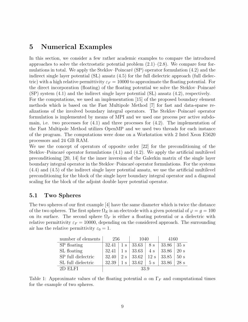
The two spheres of our first example [4] have the same diameter which is twice the distanceof the two spheres. The first sphere ΩE is an electrode with a given potential of ϕ = g = 100on its surface. The second sphere ΩF is either a floating potential or a dielectric withrelative permittivity εF = 10000, depending on the considered approach. The surroundingair has the relative permittivity ε0 = 1.
number of elements 256 1040 4160SP floating 32.41 1 s 33.63 8 s 33.86 35 sSL floating 32.41 1 s 33.63 4 s 33.86 20 sSP full dielectric 32.40 2 s 33.62 12 s 33.85 50 sSL full dielectric 32.39 1 s 33.62 5 s 33.86 28 s2D ELFI 33.9
Table 1: Approximate values of the floating potential α on ΓF and computational timesfor the example of two spheres.
9

In Table 1, we provide the approximations of the floating potential α and the computationaltimes of the four formulations for several refinement levels. For this setting an approximatesolution of an axial symmetric charge simulation solver (ELFI, [1]) is used for comparison.For the full dielectric approach, we do not determine α directly but provide the meanvalue of the potential on ΓF . Even on the finest refinement level the potential ϕF is notconstant, it has a range of 0.1983 for the indirect approach and 0.0209 for the Steklov–Poincare operator formulation.We notice that all four formulations result in good and similar approximate solutions. Onlythe indirect single layer formulation (4.5) for the full dielectric model gives a potentialwhich is not quite constant although we consider approximations of smooth objects. Wewill encounter this behavior to a greater extend in the next example.
5.2 Sphere and Bicone
Now we consider an example consisting of a sphere and a bicone [4]. Both have the samediameter and are arranged at a distance of one eighth of their diameter. One spike of thebicone points towards the sphere. The sphere ΩE is an electrode with a given potentialϕ = g = 100. The bicone ΩF has a floating potential and the exterior domain has a relativepermittivity of ε0 = 1. In Table 2, we present the approximations of the floating potentialα and the computational times. Again an approximate solution of the potential on thesurface ΓF of the cone by an axial symmetric FEM solver is used for comparison.
number of elements 384 1536 6144 24576SP floating 44.512 2 s 45.339 15 s 45.572 79 s 45.637 329 sSL floating 44.512 2 s 45.341 7 s 45.573 28 s 45.637 124 sSP full dielectric 44.512 3 s 45.340 27 s 45.573 106 s 45.636 569 sSL full dielectric 44.433 2 s 45.355 11 s 45.553 34 s 45.632 168 s2D ELFI 45.7
Table 2: Approximate values of the floating potential α on ΓF and computational timesfor the example of a sphere and a bicone.
Note that the mean value of the potential on the surface ΓF is given for the full dielectricapproaches. Therefore we analyze the range of ϕF for theses approaches in Table 3. TheSteklov–Poincare operator formulation gives an almost constant potential ϕF on the wholesurface ΓF . But we observe that the potential varies strongly for the single layer potentialansatz, even more than in the last example. The extremal values are taken at the spikesof the bicone. Such a behavior can be observed for geometries with corners and edges andresults in significant loss of accurracy, see, e.g., [2, 3].
10
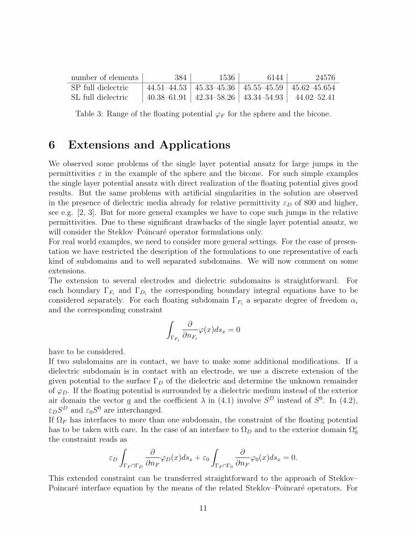
number of elements 384 1536 6144 24576SP full dielectric 44.51–44.53 45.33–45.36 45.55–45.59 45.62–45.654SL full dielectric 40.38–61.91 42.34–58.26 43.34–54.93 44.02–52.41
Table 3: Range of the floating potential ϕF for the sphere and the bicone.
6 Extensions and Applications
We observed some problems of the single layer potential ansatz for large jumps in thepermittivities ε in the example of the sphere and the bicone. For such simple examplesthe single layer potential ansatz with direct realization of the floating potential gives goodresults. But the same problems with artificial singularities in the solution are observedin the presence of dielectric media already for relative permittivity εD of 800 and higher,see e.g. [2, 3]. But for more general examples we have to cope such jumps in the relativepermittivities. Due to these significant drawbacks of the single layer potential ansatz, wewill consider the Steklov–Poincare operator formulations only.For real world examples, we need to consider more general settings. For the ease of presen-tation we have restricted the description of the formulations to one representative of eachkind of subdomains and to well separated subdomains. We will now comment on someextensions.The extension to several electrodes and dielectric subdomains is straightforward. Foreach boundary ΓFi
and ΓDithe corresponding boundary integral equations have to be
considered separately. For each floating subdomain ΓFia separate degree of freedom αi
and the corresponding constraint ∫ΓFi
∂
∂nFi
ϕ(x)dsx = 0
have to be considered.If two subdomains are in contact, we have to make some additional modifications. If adielectric subdomain is in contact with an electrode, we use a discrete extension of thegiven potential to the surface ΓD of the dielectric and determine the unknown remainderof ϕD. If the floating potential is surrounded by a dielectric medium instead of the exteriorair domain the vector a and the coefficient λ in (4.1) involve SD instead of S0. In (4.2),εDS
D and ε0S0 are interchanged.
If ΩF has interfaces to more than one subdomain, the constraint of the floating potentialhas to be taken with care. In the case of an interface to ΩD and to the exterior domain Ωc
0
the constraint reads as
εD
∫ΓF∩ΓD
∂
∂nF
ϕD(x)dsx + ε0
∫ΓF∩Γ0
∂
∂nF
ϕ0(x)dsx = 0.
This extended constraint can be transferred straightforward to the approach of Steklov–Poincare interface equation by the means of the related Steklov–Poincare operators. For
11
the indirect single layer potential ansatz, the simplification of the related constraint (4.3)seems not to be possible in general.
6.1 IEC Arrester
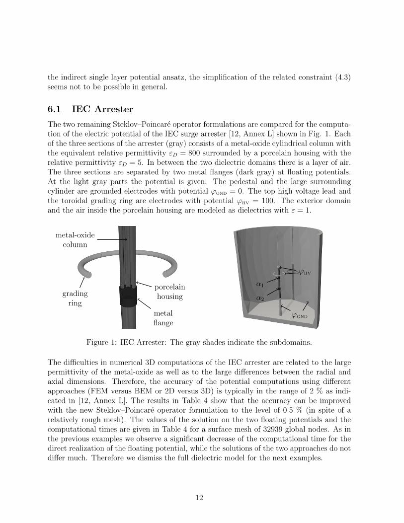
The two remaining Steklov–Poincare operator formulations are compared for the computa-tion of the electric potential of the IEC surge arrester [12, Annex L] shown in Fig. 1. Eachof the three sections of the arrester (gray) consists of a metal-oxide cylindrical column withthe equivalent relative permittivity εD = 800 surrounded by a porcelain housing with therelative permittivity εD = 5. In between the two dielectric domains there is a layer of air.The three sections are separated by two metal flanges (dark gray) at floating potentials.At the light gray parts the potential is given. The pedestal and the large surroundingcylinder are grounded electrodes with potential ϕGND = 0. The top high voltage lead andthe toroidal grading ring are electrodes with potential ϕHV = 100. The exterior domainand the air inside the porcelain housing are modeled as dielectrics with ε = 1.
gradingring
metal-oxidecolumn
metalflange
porcelainhousing α2
α1
ϕGND
ϕHV
Figure 1: IEC Arrester: The gray shades indicate the subdomains.
The difficulties in numerical 3D computations of the IEC arrester are related to the largepermittivity of the metal-oxide as well as to the large differences between the radial andaxial dimensions. Therefore, the accuracy of the potential computations using differentapproaches (FEM versus BEM or 2D versus 3D) is typically in the range of 2 % as indi-cated in [12, Annex L]. The results in Table 4 show that the accuracy can be improvedwith the new Steklov–Poincare operator formulation to the level of 0.5 % (in spite of arelatively rough mesh). The values of the solution on the two floating potentials and thecomputational times are given in Table 4 for a surface mesh of 32939 global nodes. As inthe previous examples we observe a significant decrease of the computational time for thedirect realization of the floating potential, while the solutions of the two approaches do notdiffer much. Therefore we dismiss the full dielectric model for the next examples.
12

α1 α2 timeSP floating 57.44 24.28 4559 sSP full dielectric 57.41 24.23 9659 s2D ELFI 57.62 24.42
Table 4: Approximate values of the floating potentials and computational time for the IECarrester.
6.2 Bushing
The next example models a high voltage bushing [1] shown in Fig. 2a. It consists ofa cylindrical conductor (light gray) with potential ϕHV = 100 surrounded by five thinmetallic foils embedded in a solid dielectric material (gray) with the relative permittivityεD = 5. The most outer foil (light grey) is grounded ϕGND = 0 while the other four foils(dark grey) are at floating potentials. The role of the floating foils is enforcing a uniformpotential distribution along the conical surface of the bushing. The difficult aspect ofmodeling bushings is the small thickness of the foils: for the bushing in Fig. 2a the ratiobetween the foil thickness and its axial length is in the range of 10−3. Consequently thedistance between elements created on the parallel foil surfaces is approximately 100 timessmaller than the elements’ size. In spite of these extreme geometrical relations the floatingpotentials calculated for all foils with the Steklov-Poincare operator approach show a goodagreement with the 2D solution as presented in Table 5.
α1 α2 α3 α4
SP floating 70.7 51.4 35.1 19.02D ELFI 70.8 51.4 35.0 18.9
Table 5: Approximate values of the floating potentials for the bushing.
6.3 Insulator with Partial Wetting
The last example as depicted in Fig. 2b is an isolator with embedded electrodes (lightgray) at potentials ϕHV = 100 and ϕGND = 0. The relative permittivity of the insulator(grey) is εD = 5. The upper surface of both insulator sheds is covered by a water layer(dark grey). For the operational frequency of 50–60 Hz water behaves like a conductingmaterial and can be approximated for a capacitive electrostatic field computation as anelectrode. Consequently, the two very thin domains of water (dark gray) on the insulatorsheds are modeled as electrodes at floating potentials. The geometrical dimensions of thisarrangement are as follows: electrodes’ diameter = 40 mm, distance between electrodes =14 mm, insulation thickness between electrode and air = 5 mm, shed diameter = 160 mm,shed thickness = 6 mm, and water layer thickness = 1 mm.
13

α4α3α2α1
ϕGND
ϕHV
soliddielectric
(a) Clip of the bushing.
α2
α1
ϕGND
ϕHV
insulator
(b) Clip of the insulator with partial wetting.
Figure 2: Geometric settings of the bushing and the partially wet isolator.
The solution of the floating version of the Steklov–Poincare operator approach and the 2Dsolution are given in Table 6.
α1 α2
SP floating 80.93 51.712D ELFI 81.49 52.74
Table 6: Approximate values of the floating potentials for the bushing for the insulatorwith partial wetting.
7 Conclusions
In our comparison the direct formulation based on the Steklov–Poincare interface equationturned out to be superior to the indirect single layer potential ansatz, as the results are a lotbetter in the case of large jumps of the permittivity. In particular, the indirect approachshows unphysical singularities close to edges and corners. The direct integration of thefloating potential and of the zero flux constraint proved to be faster than the approximationobtained by a dielectric media with large permittivity because of a smaller number ofdegrees of freedom and a smaller number of steps of the iterative solver. Thus the additionaleffort for the implementation of the modified system pays off.
Acknowledgement
This work was supported by the FP7 Marie Curie IAPP Project CASOPT (ControlledComponent and Assembly Level Optimisation of Industrial Devices, www.casopt.com).
14
References
[1] Z. Andjelic, B. Kristajic, S. Milojkovic, A. Blaszczyk, H. Steinbigler, andM. Wohlmuth. Integral methods for the calculation of electric fields, for applicationin high voltage engineering. Technical Report 10, Scientific Series if the InternationalBureau, Forschungszentrum Julich, 1992.
[2] Z. Andjelic, G. Of, O. Steinbach, and P. Urthaler. Boundary element methods formagnetostatic field problems: A critical view. Comput. Visual. Sci., 14:117–130,2011.
[3] Z. Andjelic, G. Of, O. Steinbach, and P. Urthaler. Fast boundary element methodsfor industrial applications in magnetostatics. In U. Langer, M. Schanz, O. Steinbach,and W.L. Wendland, editors, Fast Boundary Element Methods in Engineering andIndustrial Applications, volume 63 of Lecture Notes in Applied and ComputationalMechanics, pages 111–143. Springer, Berlin Heidelberg, 2012.
[4] A. Blaszczyk. Region-oriented bem formulation for numerical computation of electricfields. In J. Roos and L.R.J. Costa, editors, Scientific Computing in Electrical En-gineering SCEE2008, volume 14 of Mathematics in Industry, pages 69–76. Springer,Berlin, Heidelberg, 2010.
[5] A. Blaszczyk and H. Steinbigler. Region-oriented charge simulation. IEEE Trans.Magn., 30(5):2924 –2927, 1994.
[6] C. Carstensen, M. Kuhn, and U. Langer. Fast parallel solvers for symmetric boundaryelement domain decomposition equations. Numer. Math., 79(3):321–347, 1998.
[7] L. Greengard and V. Rokhlin. A fast algorithm for particle simulations. J. Comput.Phys., 73:325–348, 1987.
[8] G. C. Hsiao, O. Steinbach, and W. L. Wendland. Domain decomposition methods viaboundary integral equations. J. Comput. Appl. Math., 125(1-2):521–537, 2000.
[9] G. C. Hsiao and W. L. Wendland. Domain decomposition in boundary element meth-ods. In Fourth international symposium on domain decomposition methods for par-tial differential equations, Proc. Symp., Moscow/Russ. 1990 , pages 41–49. SIAM,Philadelphia, PA, 1991.
[10] G. C. Hsiao and W. L. Wendland. Domain decomposition via boundary elementmethods. In H. Alder et al., editor, Numerical Methods in Engineering and AppliedSciences, Part I,, pages 198–207. CIMNE, Barcelona, 1992.
[11] G. C. Hsiao and W. L. Wendland. Boundary integral equations, volume 164 of AppliedMathematical Sciences. Springer, Berlin, 2008.
15
[12] International Electrotechnical Commission. IEC Technical Standard 60099-4. Surgearresters – Part 4: Metal-oxide surge arresters without gaps for a.c. systems, 2.2edition, 2009-05.
[13] A. Konrad and M. Graovac. The finite element modeling of conductors and floatingpotentials. IEEE Trans. Magn., 32(5):4329 –4331, 1996.
[14] G. Of. An efficient algebraic multigrid preconditioner for a fast multipole boundaryelement method. Computing, 82(2-3):139–155, 2008.
[15] G. Of, O. Steinbach, and W. L. Wendland. The fast multipole method for the sym-metric boundary integral formulation. IMA J. Numer. Anal., 26(2):272–296, 2006.
[16] C. Pechstein. Finite and Boundary Element Tearing and Interconnecting Solvers forMultiscale Problems, volume 90 of Lecture Notes in Computational Science and Engi-neering. Springer, Berlin Heidelberg, 2013.
[17] F. Roman, V. Cooray, and V. Scuka. Comparison of the breakdown of rod-plane gapswith floating electrode. IEEE Trans. Diel. Elec. Insul., 5(4):622 –624, 1998.
[18] S. A. Sauter and C. Schwab. Boundary Element Methods, volume 39 of Springer Seriesin Computational Mathematics. Springer, Berlin, Heidelberg, 2011.
[19] H. Singer, H. Steinbigler, and P. Weiss. A charge simulation method for the calculationof high voltage fields. IEEE Trans. Pow. App. Syst., 93(5):1660 –1668, 1974.
[20] O. Steinbach. Artificial multilevel boundary element preconditioners. Proc. Appl.Math. Mech., 3:539–542, 2003.
[21] O. Steinbach. Numerical approximation methods for elliptic boundary value problems.Finite and boundary elements. Springer, New York, 2008.
[22] O. Steinbach and W. L. Wendland. The construction of some efficient preconditionersin the boundary element method. Adv. Comput. Math., 9(1–2):191–216, 1998.
[23] A. Toselli and O. Widlund. Domain Decomposition Methods – Algorithms and The-ory, volume 34 of Lecture Notes in Computational Mathematics. Springer, BerlinHeidelberg, 2005.
16
Erschienene Preprints ab Nummer 2012/1
2012/1 G. Of, O. Steinbach: On the ellipticity of coupled finite element and one–equationboundary element methods for boundary value problems.
2012/2 O. Steinbach: Boundary element methods in linear elasticity: Can we avoid thesymmetric formulation?
2012/3 W. Lemster, G. Lube, G. Of, O. Steinbach: Analysis of a kinematic dynamo modelwith FEM–BEM coupling.
2012/4 O. Steinbach: Boundary element methods for variational inequalities.
2012/5 G. Of, T. X. Phan, O. Steinbach: An energy space finite element approach for ellipticDirichlet boundary control problems.
2012/6 O. Steinbach, L. Tchoualag: Circulant matrices and FFT methods for the fast eval-uation of Newton potentials in BEM..
2012/7 M. Karkulik, G. Of, D. Paetorius: Convergence of adaptive 3D BEM for weaklysingular integral equations based on isotropic mesh-refinement.
2012/8 M. Bulicek, P. Pustejovska: On existence analysis of steady flows of generalizedNewtonian fluids with concentration dependent power-law index.
2012/9 U. Langer, O. Steinbach, W. L. Wendland (eds.): 10. Workshop on Fast BoundaryElement Methods in Industrial Applications. Book of Abstracts.
2012/10 O. Steinbach: Boundary integral equations for Helmholtz boundary value and trans-mission problems.
2012/11 A. Kimeswenger, O. Steinbach, G. Unger: Coupled finite and boundary elementmethods for vibro–acoustic interface problems.
2012/12 T. X. Phan, O. Steinbach: Boundary element methods for parabolic boundary con-trol problems.
2013/1 L. John, P. Pustejovska, O. Steinbach: On hemodynamic indicators related toaneurysm blood flow.
2013/2 G. Of, O. Steinbach (eds.): 9th Austrian Numerical Analysis Day. Book of Ab-stracts.