www.SandV.com10 SOUND & VIBRATION/SEPTEMBER 2013

obstacle of volume meshing on FEM no longer exists. As a consequence of this, an in-creasing number of acousti-cal engineers are embracing FEM and relying on it for their daily product design work. The FEM-based acoustic simu-lation software Actran, devel-oped by Free Field Technolo-gies (FFT), an MSC Software company, has been successfully applied in numerous intake and exhaust noise projects.2.3 In this article, we demonstrate the capabilities of Actran in predicting exhaust line noise on the public model shown in Figure 1.

Sound Transmission LossSTL is the key indicator for

acoustic performance related to pipe noise. One can nu-merically calculate the STL of a single component (for example, a muffler shown in Figure 4) or the STL of an entire exhaust

line. The technique in both cases is the same and is explained in Figure 4. A (unit) incident acoustic power from upstream is applied at the inlet of the muffler. After sound propagation in the muffler, the transmitted power downstream is calculated at the muffler’s outlet. The STL is defined as the logarithmic ratio between the incident and transmitted power (Equation 2). An acoustic non-reflective boundary condition is applied both at the outlet and inlet, to provide anechoic conditions for both propagating waves traveling downstream and any reflected waves traveling upstream. In Actran, analytical acoustic duct modes4 are coupled with the FEM mesh both at the inlet and outlet to provide the excitation of incident power, the evaluation of transmitted power, and the non-reflective conditions.

At a given frequency, a non-plane wave first occurs in larg-

Noise from both intake and exhaust lines contributes signifi-cantly to total vehicle noise. To assess the acoustic performance of automotive intake and exhaust lines, both the airborne engine noise propagating through the interior air of the line (known as pipe noise) and the structure-borne noise radiated by the line’s surface shell structure (shell noise) should be evaluated. This ar-ticle describes the study of both pipe and shell noise of a complex exhaust line using a finite-element method (FEM), coupled with a transfer matrix method (TMM).

In automotive NVH, intake noise and exhaust noise are important contributors to total vehicle noise. Today, as engine noise is increas-ingly controlled with new technologies, intake and exhaust noise emerge and, as shown in Table 1, reach the same level as engine noise in the typical truck used as an example. As a consequence, both automotive OEMs and suppliers pay increasing attention to intake and exhaust noises.

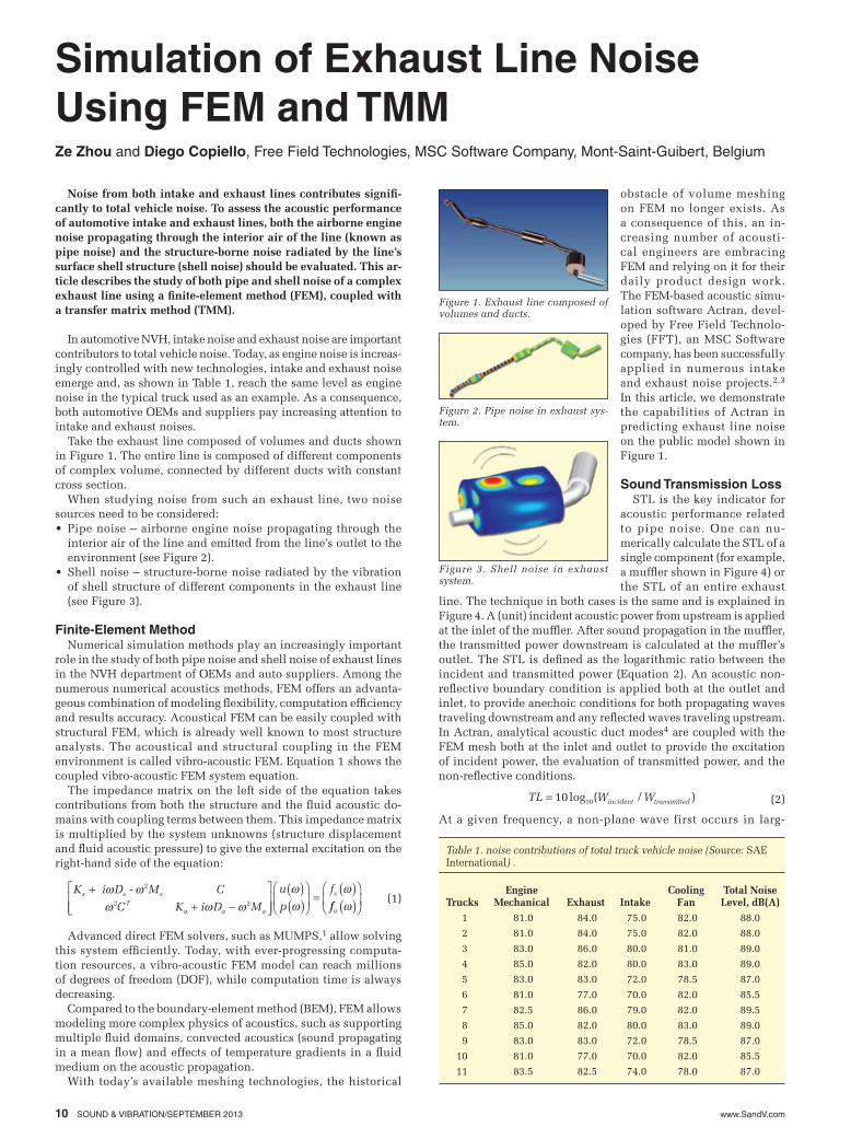
Take the exhaust line composed of volumes and ducts shown in Figure 1. The entire line is composed of different components of complex volume, connected by different ducts with constant cross section.

When studying noise from such an exhaust line, two noise sources need to be considered:• Pipe noise – airborne engine noise propagating through the

interior air of the line and emitted from the line’s outlet to the environment (see Figure 2).

• Shell noise – structure-borne noise radiated by the vibration of shell structure of different components in the exhaust line (see Figure 3).

Finite-Element MethodNumerical simulation methods play an increasingly important

role in the study of both pipe noise and shell noise of exhaust lines in the NVH department of OEMs and auto suppliers. Among the numerous numerical acoustics methods, FEM offers an advanta-geous combination of modeling flexibility, computation efficiency and results accuracy. Acoustical FEM can be easily coupled with structural FEM, which is already well known to most structure analysts. The acoustical and structural coupling in the FEM environment is called vibro-acoustic FEM. Equation 1 shows the coupled vibro-acoustic FEM system equation.

The impedance matrix on the left side of the equation takes contributions from both the structure and the fluid acoustic do-mains with coupling terms between them. This impedance matrix is multiplied by the system unknowns (structure displacement and fluid acoustic pressure) to give the external excitation on the right-hand side of the equation:

Advanced direct FEM solvers, such as MUMPS,1 allow solving this system efficiently. Today, with ever-progressing computa-tion resources, a vibro-acoustic FEM model can reach millions of degrees of freedom (DOF), while computation time is always decreasing.

Compared to the boundary-element method (BEM), FEM allows modeling more complex physics of acoustics, such as supporting multiple fluid domains, convected acoustics (sound propagating in a mean flow) and effects of temperature gradients in a fluid medium on the acoustic propagation.

With today’s available meshing technologies, the historical

Simulation of Exhaust Line Noise Using FEM and TMM

(1)K i D M C

C K i D M

u

p

fs s sT

a a a

s++ -

È

ÎÍÍ

˘

˚˙˙

( )( )

Ê

ËÁ

ˆ

¯˜ =

( ) w ww w w

ww

w- 2

2 2 ffa w( )Ê

ËÁ

ˆ

¯˜

(2)TL W Wincident transmitted= 10 10log ( / )

Ze Zhou and Diego Copiello, Free Field Technologies, MSC Software Company, Mont-Saint-Guibert, Belgium

Table 1. noise contributions of total truck vehicle noise (Source: SAE International) .

Engine Cooling Total NoiseTrucks Mechanical Exhaust Intake Fan Level, dB(A)

1 81.0 84.0 75.0 82.0 88.0 2 81.0 84.0 75.0 82.0 88.0 3 83.0 86.0 80.0 81.0 89.0 4 85.0 82.0 80.0 83.0 89.0 5 83.0 83.0 72.0 78.5 87.0 6 81.0 77.0 70.0 82.0 85.5 7 82.5 86.0 79.0 82.0 89.5 8 85.0 82.0 80.0 83.0 89.0 9 83.0 83.0 72.0 78.5 87.010 81.0 77.0 70.0 82.0 85.511 83.5 82.5 74.0 78.0 87.0

Figure 1. Exhaust line composed of volumes and ducts.

Figure 2. Pipe noise in exhaust sys-tem.

Figure 3. Shell noise in exhaust system.

www.SandV.com SOUND & VIBRATION/SEPTEMBER 2013 11

Figure 7. Transfer matrix of entire line as a product of transfer matrices of its subcomponents.

er volumes or in ducts with larger cross-sections. This is demonstrated in Figure 5. One observes a plane wave in the inlet and outlet ducts, but a non-plane wave in the muffler volume.

Transfer Matrix MethodTMM is an analytical method

that allows assessing the STL of an entire exhaust line by combining acoustic transfer matrices of each of its constitu-ent sub-components. Typically, a sub-component’s transfer matrix is expressed in Equa-tion 3, where I and R are the incident and transmitted waves for acoustic propagations in both directions (see Figure 6. Incident and transmitted waves in both directions in a subcom-ponent for its transfer matrix definition.).

The transfer matrix of an entire line T is assembled as the product of all the transfer matrices of its sub-components T1, T2, T3, etc. as shown in Figure 7. Transfer matrix of entire line as a product of transfer matrices of its subcomponents..

A TMM utility is implemented in the Actran software. The transfer matrices of the sub-components are calculated individu-ally using FEM. The combined FEM computation effort on all the sub-components is less than the total computation effort for the entire line. So in the study of exhaust noise, the combination of FEM and TMM offers both 3D capabilities for modeling pipe noise and shell noise and enhanced simulation efficiency.

Using TMM, the source amplitude and impedance can be plugged upstream to the entire line to calculate the sound pressure level transmitted from the outlet as shown in Figure 8. The source reflection factor is related to the source impedance by Equation 4:

The reflection factor depends on the nature of the source. For a source imposing acoustic pressure, the reflection factor is –1, meaning total pressure reflection with 180o phase change. For a source imposing acoustic velocity, the refection factor is 1, mean-ing total reflection without phase change. For a real source from the engine, the reflection factor could be frequency dependent, since the source tends to be a velocity source at low frequencies and pressure source at higher frequencies.

Perforation SimulationPerforated plates are often used in muffler design. The acoustic

propagation through the perforation can be simulated by mesh-ing the holes of the perforation, as shown in Figure 9. A simpler, more efficient way to model perforation is to replace the mesh by an equivalent acoustic transfer admittance relation across the perforated plate as shown in Figure 10.

The transfer admittance matrix based on Mechel’s formula is expressed by Equation 5. Vn and p are normal acoustic velocity and pressure on both sides of the perforation as shown in Figure 11. The assumption of Mechel’s formula is Vn1 = Vn2. Under such assumption, the calcualted admittance (Ap) is expressed in Equa-tion 6. The different terms in Equation 6 are explained in Figure 12. Among these terms, the correction factor is determined by the the perforation pattern of the holes. Figure 13 provides the cor-rection factor equations for hole patterns with square layout and hexagonal layout.

Porous Material Simulation

A porous material is usu-ally used in muffler design to provide acoustic absorption to sound traveling through the muffler. In Actran, the porous material can be modeled using the Biot formulation. To model the porous-elastic behavior, the complete set of Biot properties need to be provided, including:•Fluidproperties–density,compressibility, viscosity, ther-mal conductivity, specific heat values•Elasticparameters–soliddensity, Young’s modulus, Pois-son ratio•Fluid-skeletonproperties– porosity, flow resistivity, tor-tuosity, etc.•Micromodelparameters–viscous length, thermal length

Simplified porous formula-tions, requiring fewer proper-ties of porous material, are also available. The most well-known simplifications are the rigid porous formulation assuming rigid skeleton; the lumped po-rous formulation assuming ex-tremely soft but heavy skeleton; and the empirical models such as Delany-Bazley porous model and the Miki porous model.5,6

Effects of Flow and Temperature Gradient

During sound propagation across ducts and mufflers, the non-uniform background flow modifies the propagation. The governing equation for this sound propagation is the convected Helmholtz equation.

The temperature gradient in the propagating medium changes the local air density and acoustic wave length and therefore modi-fies the sound propagation. In a FEM model, effects of flow and temperature can be taken into account by defining flow speed and temperature values on each FEM node.

Numerical ExamplesSTL of Muffler. STL is calculated for the muffler components in

(3)I

R

I

R1

1

2

2

ÏÌÓÔ

¸˝Ô

=È

ÎÍ

˘

˚˙

ÏÌÓÔ

¸˝Ô

È

ÎÍ

˘

˚˙ =

a bg d

a bg d

* TTransfer matrix of the system

(4)Z crr

rZ cZ c

=+-

¤ =-+

rrr

*11

(5)nn

n

n

p p

p p

A A

A A

p

p1

2

1

2

È

ÎÍ

˘

˚˙ =

-

-È

ÎÍÍ

˘

˚˙˙

È

ÎÍ

˘

˚˙

(6)

A R j X

R fa

X f l l

p p p

p

p

= +( )= +Ê

ËÁˆ¯

= +

1

116 1

12

22

0

/ .

( )

ep hr

ep r D

Figure 4. Sound transmission loss of muffler.

Figure 6. Incident and transmitted waves in both directions in a sub-component for its transfer matrix definition.

I1

R1

I2

R2

Figure 5. Non-plane (3D) wave occurs first in larger volume or ducts with large cross-section.

Figure 8. Source characterized by amplitude (C) and reflection fac-tor (r).

I1

R1

C

r

Figure 9. Acoustic meshing of a per-forated plate.

Figure 10. Equivalent acoustic trans-fer admittance across perforation.

Figure 11. Normal acoustic veloc-ity and pressure on two sides of perforation.

Figure 12. Explanation of different terms in calculating transfer admit-tance.

where:

porosity

correction fact

e = == =

f a d

l g a d

( , )

( , )D oor

dynamic viscosity

air density

hr

==

l

2a

d

I1

R1

I2

R2

T1 T2 T3

www.SandV.com12 SOUND & VIBRATION/SEPTEMBER 2013

Entire Exhaust Line Model-ing and TMM. The entire line is composed of three different acoustic volumes, connected by ducts. The third volume is the muffler studied in the previous section. Here, the muffler has the perforated sheet but no po-rous material in the expansion chamber.

The transmitted power is computed at the outlet with free-field radiation conditions, provided by Inifnite Elements, and shown in Figure 20. We observe in the same figure that the free-field outlet condition generates acoustic reflection, as

a duct section change occurs connecting the finite cross-section with the free-field infinite cross section.

The acoustic pressure at 2000 Hz is shown in Figure 21. One observes 1D sound propagation behavior in the ducts and in the first two volumes. In the third volume, 3D behavior occurs.

In the TMM model, the exhaust line is divided into four sub-components corresponding to the three acoustic volumes and the free-field outlet condition shown in Figure 22. Figure 23 shows a perfect correlation of STL curves calcualted on the entire line model (frequency step = 50 Hz) and on the model employing the TMM technique (frequency step = 100 Hz), respectively.

Computation Statistics. The acoustic mesh contains about 2 mil-lion nodes for the entire line in a single FEM model valid up to 2000 Hz. The calculation time with the Actran solver is one hour per frequency on a standard workstation (the RAM requirement is 20 GB). Using TMM and solving the line sub-components separately, the computation time per frequency is reduced to 30 minutes, and the RAM consumption is reduced to 10 GB (required by the largest sub-component – the muffler volume). Using frequency paralleliza-tion, the computation time per frequency can be divided by the number of parallel processes.

Plugging Engine Source to TMM. The TMM is coupled with a unit-source amplitude with three reflection factors (0, –1 and 1) to calculate the SPL at a virtual microphone 1 m away from the outlet. The SPL results with up to 2000 Hz and a frequency step of 100 Hz are shown in Figure 24.

ConclusionsWe presented a complex exhaust noise problem in this article.

The complexity was related to many factors, namely the irregular

the exhaust line. Five configura-tions are compared:•Baselinemuffler,whichistheexpansion chamber shown in Figure 14.•Mufflerwithperforation,separating the central duct and the expansion chamber shown in Figure 15.•Mufflerwithperforationandporous material fill in the ex-pansion chamber; the porous material is modeled using rigid porous formulation.•Mufflerwithperforation,porous material, and flow effect shown in Figure 16.•Mufflerwithperforation,po-rous material, and temperature effect shown in Figure 16.

The STL curves of different configurations are shown in Fig-ure 17. In the baseline muffler, under 500~600 Hz, the sound

propagation has a 1D planar behavior. As the frequency increases, 3D behavior occurs. The perforated sheet changes the STL of the baseliner muffler, but not significantly. When the porous material is added to the expansion chamber, the STL curve becomes much smoother, with increased levels in the higher frequency range. The effect of flow and temperature gradients are relatively important.

Muffler Shell Noise. The shell noise caused by muffler shell vibration is calculated using a two-step approach. In the first step, the coupled problem of interior air and muffler shell is calculated. The shell vibration is obtained, as shown in Figure 18. In the same figure, the infinite elements allowing the shell noise radiation and the far-field virtual microphones are shown. The sound pressure level directivity around the microphone circle at 500 and 1000 Hz is shown in Figure 19.

Figure 14. Expansion chamber of baseline muffler.

Figure 15. Muffler with perforation.

Figure 13. Correction factor of perforation transfer admittance; square grid (top) and hexagonal grid (bottom).

(b) Hexagonal grid

d

ep

=◊

◊

◊ -ÊËÁ

ˆ¯

< <

◊ -

6

5 3

0 85 1 2 52 0 0 25

0 668 1 2

2

2

a

d

l

aad

ad

a

D. . .

.

.. . .0 0 25 0 5ad

ad

ÊËÁ

ˆ¯

< <

Ï

ÌÔÔ

ÓÔÔ

¸

˝ÔÔ

˛ÔÔ

ep

=◊

◊ -ÊËÁ

ˆ¯

< <

◊ -

ad

l

aad

ad

aad

2

2

0 85 1 2 34 0 0 25

0 668 1 1 9

D. . .

. .

ÊÊËÁ

ˆ¯

< <

Ï

ÌÔÔ

ÓÔÔ

¸

˝ÔÔ

˛ÔÔ 0 25 0 5. .

ad

(a) Square grid

d

Figure 17. Sound transmission loss of different muffler models.

Figure 16. Flow speed in central duct, in mm/s ((left); temperature in central duct, in K (right).

Figure 18. Shell vibration at 1000 Hz, infinite elements and virtual microphones.

www.SandV.com SOUND & VIBRATION/SEPTEMBER 2013 13

geometry, the presence of both a perforated sheet and porous mate-rial, and a non-uniform flow involving both con-vection and temperature gradients. This article demonstrates the nu-merical simulation of such complex exhaust line noise using FEM and TMM, both avail-able in the Actran soft-ware.

References1. MUMPS Solver: http://mumps.ensaeeiht.fr/.

2. Mitsubishi Motors, “Exhaust System Modeling Using a Transfer Matrix Method Coupled to Actran,” Actran Users Conference, Belgium, 2010.

3. T. Le Bourdon, et al., “Vibro-Acoustic Simulation of Intake Air Filter Using a Hybrid Modal Physical Coupling,” ISNVH 2012-01-1549.

4. Analytical Duct Modes: J. M. Tyler and T. G. Sofrin, “Axial Flow Com-pressor Noise Studies,” SAE Transactions, Vol. 70, pp. 309-332, 1962.

5. M. E. Delany and E. N. Bazley, “Acoustical Characteristics Of Fibrous Absorbent Materials,” Report of the National Physical Laboratory, Aero-dynamics division, March 1969.

Figure 19. Far-field directivity at 500 Hz (left) and 1000 Hz (right).

Figure 20. Infinite elements at outlet allowing free-field radiation.

Figure 21. Acoustic pressure in exhaust line at 2000 Hz.

Figure 22. Transfer matrix method components.

The author may be reached at: ze.zhou@fft.be.

Figure 23. Sound transmission loss of entire exhaust line.

Figure 24. Sound pressure level on exterior microphone due to unit source with different reflection factors.

6. Y. Miki, “Acoustical Properties of Porous Materials – Modifications of Delany-Bazley Models,” J. Acoust. Soc. Jpn. 11(1), pp. 19-24 1990.