simulation of adaptive array algorithms for cdma...
TRANSCRIPT

Simulation of Adaptive Array Algorithms for
CDMA Systems
by
Zhigang Rong
Thesis submitted to the faculty of the
Virginia Polytechnic Institute and State University
in partial fulfillment of the requirements for the degree of
MASTER OF SCIENCE
in
Electrical Engineering
c©Zhigang Rong and VPI & SU 1996
APPROVED:
Dr. Theodore S. Rappaport, Chairman
Dr. Jeffrey H. Reed Dr. Brian D. Woerner
September, 1996
Blacksburg, Virginia
Keywords: Adaptive Antennas, Adaptive Algorithm, CDMA
Simulation of Adaptive Array Algorithms for CDMA
Systems
by
Zhigang Rong
Committee Chairman: Dr. Theodore S. Rappaport
Bradley Department of Electrical Engineering
(ABSTRACT)
The increasing demand for mobile communication services without a corresponding in-
crease in RF spectrum allocation motivates the need for new techniques to improve spectrum
utilization. The CDMA and adaptive antenna array are two approaches that shows real
promise for increasing spectrum efficiency. In this research, we investigate the performance
of different blind adaptive array algorithms in the CDMA systems. Two novel algorithms,
least-squares despread respread multitarget array (LS-DRMTA) and least-squares despread
respread multitarget constant modulus algorithm (LS-DRMTCMA), are developed, and a
MATLABTM simulation testbed is created to compare the performance of these two novel
algorithms with those of the multitarget least-squares constant modulus algorithm (MT-
LSCMA) and multitarget steepest-descent decision-directed (MT-SDDD) algorithm. It is
shown from the simulation results that these two novel algorithms can outperform the
other algorithms in all the test situations (e. g., AWGN channel, timing offset case, fre-
quency offset case, and multipath environment). It is also shown that these two algorithms
have less complexity and can converge faster than the other algorithms.

ACKNOWLEDGEMENTS
I would like to thank my academic advisor, Dr. Theodore S. Rappaport, for the invalu-
able support, guidance and encouragement he has provided over the past year. I thank my
committee members, Dr. Jeffrey H. Reed and Dr. Brian D. Woerner, for carefully review-
ing my thesis report and providing useful suggestions.
I wish to thank Paul Petrus for his help and fruitful discussion during the course of
this research. I would like to thank him for the suggestion of varying the coefficients in the
LS-DRMTCMA. I would also thank Tom Biedka for his valuable advice and suggestions in
the simulation of MT-LSCMA.
I would like to thank Nitin Mangalvedhe, Francis Dominique, and Keith Blankenship
for their help throughout the course of this work. I also thank Prab Koushik for providing
the necessary support for my computational demands.
I wish to thank the Defense Advanced Research Projects Agency’s (DARPA) Global
Mobile (GLOMO) program for providing financial support for this work.
I would like to thank all my friends who have provided me all kinds of help in the last
two years.
Most of all, I would like to thank my parents and family for their love and encouragement.
I could not have completed my degree without their continuous and immeasurable support.
iii

TABLE OF CONTENTS
1 Introduction 1
1.1 Motivation . . . . . . . . . . . . . . . . . . . . . . . . . . . . . . . . . . . . 1
1.2 Objective and Outline of Thesis . . . . . . . . . . . . . . . . . . . . . . . . . 2
2 Fundamentals of Adaptive Antenna Arrays 4
2.1 Uniformly Spaced Linear Array . . . . . . . . . . . . . . . . . . . . . . . . . 5
2.2 Beamforming and Spatial Filtering . . . . . . . . . . . . . . . . . . . . . . . 11
2.3 Beampattern and Element Spacing . . . . . . . . . . . . . . . . . . . . . . . 13
2.4 Adaptive Arrays . . . . . . . . . . . . . . . . . . . . . . . . . . . . . . . . . 21
2.5 Summary . . . . . . . . . . . . . . . . . . . . . . . . . . . . . . . . . . . . . 23
3 Overview of Adaptive Beamforming Algorithms 24
3.1 Introduction . . . . . . . . . . . . . . . . . . . . . . . . . . . . . . . . . . . . 24
3.2 Non-blind Adaptive Algorithms . . . . . . . . . . . . . . . . . . . . . . . . . 24
3.2.1 Wiener Solution . . . . . . . . . . . . . . . . . . . . . . . . . . . . . 25
3.2.2 Method of Steepest-Descent . . . . . . . . . . . . . . . . . . . . . . . 26
3.2.3 Least-Mean-Squares Algorithm . . . . . . . . . . . . . . . . . . . . . 28
3.2.4 Recursive Least-Squares Algorithm . . . . . . . . . . . . . . . . . . . 29
3.3 Blind Adaptive Algorithms . . . . . . . . . . . . . . . . . . . . . . . . . . . 31
3.3.1 Algorithms Based on Estimation of DOAs of Received Signals . . . . 31
3.3.2 Algorithms Based on Property-Restoral Techniques . . . . . . . . . . 32
3.3.3 Algorithms Based on Discrete-Alphabet Structure of Digital Signal . 43
3.3.4 Other Blind Beamforming Algorithms . . . . . . . . . . . . . . . . . 43
3.4 Summary . . . . . . . . . . . . . . . . . . . . . . . . . . . . . . . . . . . . . 45
iv

CONTENTS
4 Adaptive Beamforming Algorithms Used in Simulation 46
4.1 Introduction . . . . . . . . . . . . . . . . . . . . . . . . . . . . . . . . . . . . 46
4.2 Multitarget Beamformer . . . . . . . . . . . . . . . . . . . . . . . . . . . . . 46
4.3 Multitarget Least-Squares Constant Modulus Algorithm . . . . . . . . . . . 49
4.3.1 Gram-Schmidt Orthogonalization . . . . . . . . . . . . . . . . . . . . 49
4.3.2 Phase Ambiguity . . . . . . . . . . . . . . . . . . . . . . . . . . . . . 52
4.3.3 Sorting Procedure . . . . . . . . . . . . . . . . . . . . . . . . . . . . 53
4.4 Multitarget Decision-Directed Algorithm . . . . . . . . . . . . . . . . . . . . 57
4.5 Least-Squares Despread Respread Multitarget Array . . . . . . . . . . . . . 58
4.5.1 Derivation of LS-DRMTA . . . . . . . . . . . . . . . . . . . . . . . . 59
4.5.2 Advantages of LS-DRMTA . . . . . . . . . . . . . . . . . . . . . . . 65
4.6 Least-Squares Despread Respread Multitarget Constant Modulus Algorithm 67
4.6.1 Derivation of LS-DRMTCMA . . . . . . . . . . . . . . . . . . . . . . 67
4.6.2 Advantages of LS-DRMTCMA . . . . . . . . . . . . . . . . . . . . . 72
4.7 Summary . . . . . . . . . . . . . . . . . . . . . . . . . . . . . . . . . . . . . 72
5 Simulation Results and Discussion 73
5.1 Introduction . . . . . . . . . . . . . . . . . . . . . . . . . . . . . . . . . . . . 73
5.2 Description of System Parameters . . . . . . . . . . . . . . . . . . . . . . . 73
5.3 Simulation Results in AWGN Channel . . . . . . . . . . . . . . . . . . . . . 74
5.3.1 General Result . . . . . . . . . . . . . . . . . . . . . . . . . . . . . . 75
5.3.2 BER Performance for AWGN Channel . . . . . . . . . . . . . . . . . 79
5.4 BER Performance in Timing Offset Case . . . . . . . . . . . . . . . . . . . . 92
5.5 BER Performance in Frequency Offset Case . . . . . . . . . . . . . . . . . . 94
5.6 BER Performance and Coefficients in LS-DRMTCMA . . . . . . . . . . . . 103
5.7 BER Performance in Multipath Environment . . . . . . . . . . . . . . . . . 104
5.8 Conclusion . . . . . . . . . . . . . . . . . . . . . . . . . . . . . . . . . . . . 112
v

CONTENTS
6 Conclusions and Future Work 113
6.1 Conclusions . . . . . . . . . . . . . . . . . . . . . . . . . . . . . . . . . . . . 113
6.2 Future Work . . . . . . . . . . . . . . . . . . . . . . . . . . . . . . . . . . . 114
A Differentiation with Respect to a Vector 116
A.1 Basic Definitions . . . . . . . . . . . . . . . . . . . . . . . . . . . . . . . . . 116
A.2 Examples . . . . . . . . . . . . . . . . . . . . . . . . . . . . . . . . . . . . . 118
References 119
Programs 125
vi

LIST OF FIGURES
2.1 Illustration of a plane wave incident on a uniformly spaced linear array from
direction θ. . . . . . . . . . . . . . . . . . . . . . . . . . . . . . . . . . . . . 6
2.2 A narrowband beamformer forms a linear combination of the sensor outputs. 12
2.3 A wideband beamformer samples the signal in both space and time. . . . . 14
2.4 A FIR filter used to perform filtering in the time domain. . . . . . . . . . . 15
2.5 Beampattern for an equal-weight beamformer. In this case, the number of el-
ements is equal to 8, and the element spacing is half of the carrier wavelength.
The plot is generated by Programs [P1] and [P2]. . . . . . . . . . . . . . . . 19
2.6 The same beampattern as shown in Figure 2.5 with polar coordinate plot in
azimuth. The plot is generated by Programs [P1] and [P2]. . . . . . . . . . 19
2.7 A simple narrowband adaptive array. . . . . . . . . . . . . . . . . . . . . . . 22
4.1 A multitarget adaptive beamformer with M antenna elements and Q output
ports. . . . . . . . . . . . . . . . . . . . . . . . . . . . . . . . . . . . . . . . 48
4.2 Illustration of a multitarget LS-CMA adaptive array. . . . . . . . . . . . . . 50
4.3 Illustration of sorting procedure in MT-LSCMA for a CDMA system. . . . 55
4.4 Structure of a beamformer using LS-DRMTA. . . . . . . . . . . . . . . . . . 60
4.5 LS-DRMTA block diagram for user i. . . . . . . . . . . . . . . . . . . . . . 61
4.6 Structure of a beamformer using LS-DRMTCMA. . . . . . . . . . . . . . . 68
4.7 LS-DRMTCMA block diagram for user i. . . . . . . . . . . . . . . . . . . . 69
5.1 Illustration of eight users with DOAs equally spaced between −70◦ and 90◦. 75
vii

LIST OF FIGURES
5.2 Beampatterns corresponding to different users generated by using LS-DRMTCMA.
∗ denotes user in the system. The signal parameters are shown in Table 5.1.
This plot is generated by Programs [P4] and [P5]. . . . . . . . . . . . . . . . 76
5.3 Beampatterns corresponding to different users generated by using LS-DRMTCMA
(cntd.). This plot is generated by Programs [P4] and [P5]. . . . . . . . . . . 76
5.4 Signal constellation of user 5 before the beamformer processing. The signal
parameters are shown in Table 5.1. This plot is generated by Programs [P4]
and [P6]. . . . . . . . . . . . . . . . . . . . . . . . . . . . . . . . . . . . . . . 78
5.5 Signal constellation of user 5 after the beamformer processing. The signal
parameters are shown in Table 5.1. This plot is generated by Programs [P4]
and [P6]. . . . . . . . . . . . . . . . . . . . . . . . . . . . . . . . . . . . . . . 78
5.6 Original signal waveform of user 5. The signal parameters are shown in Table
5.1. This plot is generated by Programs [P4] and [P7]. . . . . . . . . . . . . 80
5.7 Corrupted signal waveform of user 5. The signal parameters are shown in
Table 5.1. This plot is generated by Programs [P4] and [P7]. . . . . . . . . 80
5.8 Reconstructed signal waveform of user 5. The signal parameters are shown
in Table 5.1. This plot is generated by Programs [P4] and [P7]. . . . . . . . 81
5.9 Convergence curve for MT-SDDD in port 6 of the beamformer. The signal
parameters are shown in Table 5.1. This plot is generated by Programs [P4]
and [P8]. . . . . . . . . . . . . . . . . . . . . . . . . . . . . . . . . . . . . . . 81
5.10 Convergence curve for LS-DRMTCMA in port 6 of the beamformer. The
LS-DRMTCMA is described in equations (4.46)-(4.51). The data block size
in each iteration is equal to 60. The signal parameters are shown in Table
5.1. This plot is generated by Programs [P4] and [P9]. . . . . . . . . . . . . 83
5.11 DOA distribution of all the users for both the non-crowded and crowded cases. 83
viii

LIST OF FIGURES
5.12 BER performance of different adaptive algorithms. In this case, Eb/N0 = 8
dB, the DOAs of all the users are equally spaced between −70◦ and 90◦. The
ratio of the coefficients aPN/aCM used in the LS-DRMTCMA is set to 2.
This plot is generated by Programs [P10] and [P12]. . . . . . . . . . . . . . 84
5.13 BER performance of different adaptive algorithms. In this case, Eb/N0 = 8
dB, the DOAs of all the users are equally spaced between 0◦ and 90◦. The
ratio of the coefficients aPN/aCM used in the LS-DRMTCMA is set to 2.
This plot is generated by Programs [P10] and [P12]. . . . . . . . . . . . . . 84
5.14 Beampattern of user 5 generated by using LS-DRMTCMA. In this case,
Eb/N0 = 8 dB, the number of users is equal to 8, the DOAs of all the
users are equally spaced between −70◦ and 90◦. The ratio of the coefficients
aPN/aCM used in the LS-DRMTCMA is set to 2. This plot is generated by
Programs [P4] and [P13]. . . . . . . . . . . . . . . . . . . . . . . . . . . . . 86
5.15 Beampattern of user 5 generated by using MT-SDDD. In this case, Eb/N0 =
8 dB, the number of users is equal to 8, the DOAs of all the users are equally
spaced between −70◦ and 90◦. The ratio of the coefficients aPN/aCM used
in the LS-DRMTCMA is set to 2. This plot is generated by Programs [P4]
and [P13]. . . . . . . . . . . . . . . . . . . . . . . . . . . . . . . . . . . . . . 86
5.16 Beampattern of user 4 generated by using LS-DRMTCMA. In this case,
Eb/N0 = 8 dB, the number of users is equal to 8, the DOAs of all the
users are equally spaced between −70◦ and 90◦. The ratio of the coefficients
aPN/aCM used in the LS-DRMTCMA is set to 2. This plot is generated by
Programs [P4] and [P13]. . . . . . . . . . . . . . . . . . . . . . . . . . . . . 88
5.17 Beampattern of user 4 generated by using LS-DRMTCMA. In this case,
Eb/N0 = 8 dB, the number of users is equal to 8, the DOAs of all the
users are equally spaced between 0◦ and 90◦. The ratio of the coefficients
aPN/aCM used in the LS-DRMTCMA is set to 2. This plot is generated by
Programs [P4] and [P13]. . . . . . . . . . . . . . . . . . . . . . . . . . . . . 88
ix

LIST OF FIGURES
5.18 BER performance of different adaptive algorithms. In this case, Eb/N0 = 4
dB, the DOAs of all the users are equally spaced between −70◦ and 90◦. The
ratio of the coefficients aPN/aCM used in the LS-DRMTCMA is set to 2.
This plot is generated by Programs [P10] and [P12]. . . . . . . . . . . . . . 90
5.19 BER performance of different adaptive algorithms. In this case, Eb/N0 = 4
dB, the DOAs of all the users are equally spaced between 0◦ and 90◦. The
ratio of the coefficients aPN/aCM used in the LS-DRMTCMA is set to 2.
This plot is generated by Programs [P10] and [P12]. . . . . . . . . . . . . . 90
5.20 Beampattern of user 4 generated by using LS-DRMTCMA in the non-crowded
DOA case. In this case, Eb/N0 = 4 dB, the number of users is equal to 4, the
DOAs of all the users are equally spaced between −70◦ and 90◦. The ratio of
the coefficients aPN/aCM used in the LS-DRMTCMA is set to 2. This plot
is generated by Programs [P4] and [P13]. . . . . . . . . . . . . . . . . . . . 91
5.21 Beampattern of user 4 generated by using LS-DRMTCMA in the crowded
DOA case. In this case, Eb/N0 = 4 dB, the number of users is equal to 4, the
DOAs of all the users are equally spaced between 0◦ and 90◦. The ratio of
the coefficients aPN/aCM used in the LS-DRMTCMA is set to 2. This plot
is generated by Programs [P4] and [P13]. . . . . . . . . . . . . . . . . . . . 91
5.22 BER performance of different adaptive algorithms in timing offset case. In
this case, Eb/N0 = 8 dB, To = 0.25Tc, the DOAs of all the users are equally
spaced between −70◦ and 90◦. The ratio of the coefficients aPN/aCM used
in the LS-DRMTCMA is set to 2. This plot is generated by Programs [P14]
and [P15]. . . . . . . . . . . . . . . . . . . . . . . . . . . . . . . . . . . . . . 93
5.23 BER performance of different adaptive algorithms in timing offset case. In
this case, Eb/N0 = 8 dB, To = 0.25Tc, the DOAs of all the users are equally
spaced between 0◦ and 90◦. The ratio of the coefficients aPN/aCM used in
the LS-DRMTCMA is set to 2. This plot is generated by Programs [P14]
and [P15]. . . . . . . . . . . . . . . . . . . . . . . . . . . . . . . . . . . . . . 93
x

LIST OF FIGURES
5.24 BER performance of different adaptive algorithms in timing offset case. In
this case, Eb/N0 = 8 dB, To = 0.5Tc, the DOAs of all the users are equally
spaced between −70◦ and 90◦. The ratio of the coefficients aPN/aCM used
in the LS-DRMTCMA is set to 2. This plot is generated by Programs [P14]
and [P16]. . . . . . . . . . . . . . . . . . . . . . . . . . . . . . . . . . . . . . 95
5.25 BER performance of different adaptive algorithms in timing offset case. In
this case, Eb/N0 = 8 dB, To = 0.5Tc, the DOAs of all the users are equally
spaced between 0◦ and 90◦. The ratio of the coefficients aPN/aCM used in
the LS-DRMTCMA is set to 2. This plot is generated by Programs [P14]
and [P16]. . . . . . . . . . . . . . . . . . . . . . . . . . . . . . . . . . . . . . 95
5.26 BER vs. timing offset for different adaptive algorithms. In this case, Eb/N0 =
8 dB, the number of users is equal to 10, the DOAs of all the users are equally
spaced between −70◦ and 90◦. The ratio of the coefficients aPN/aCM used
in the LS-DRMTCMA is set to 2. This plot is generated by Programs [P14]
and [P17]. . . . . . . . . . . . . . . . . . . . . . . . . . . . . . . . . . . . . . 96
5.27 BER vs. timing offset for different adaptive algorithms. In this case, Eb/N0 =
8 dB, the number of users is equal to 10, the DOAs of all the users are equally
spaced between 0◦ and 90◦. The ratio of the coefficients aPN/aCM used in
the LS-DRMTCMA is set to 2. This plot is generated by Programs [P14]
and [P17]. . . . . . . . . . . . . . . . . . . . . . . . . . . . . . . . . . . . . . 96
5.28 BER performance of different adaptive algorithms in frequency offset case. In
this case, Eb/N0 = 8 dB, Fo = 100 Hz, the DOAs of all the users are equally
spaced between −70◦ and 90◦. The ratio of the coefficients aPN/aCM used
in the LS-DRMTCMA is set to 2. The maximum phase shift φa between
two consecutive adaptation period is set to 0.2π. This plot is generated by
Programs [P18] and [P19]. . . . . . . . . . . . . . . . . . . . . . . . . . . . . 98
xi

LIST OF FIGURES
5.29 BER performance of different adaptive algorithms in frequency offset case.
In this case, Eb/N0 = 8 dB, Fo = 100 Hz, the DOAs of all the users are
equally spaced between 0◦ and 90◦. The ratio of the coefficients aPN/aCM
used in the LS-DRMTCMA is set to 2. The maximum phase shift φa between
two consecutive adaptation period is set to 0.2π. This plot is generated by
Programs [P18] and [P19]. . . . . . . . . . . . . . . . . . . . . . . . . . . . . 98
5.30 BER performance of different adaptive algorithms in frequency offset case. In
this case, Eb/N0 = 8 dB, Fo = 500 Hz, the DOAs of all the users are equally
spaced between −70◦ and 90◦. The ratio of the coefficients aPN/aCM used
in the LS-DRMTCMA is set to 2. The maximum phase shift φa between
two consecutive adaptation period is set to 0.2π. This plot is generated by
Programs [P18] and [P19]. . . . . . . . . . . . . . . . . . . . . . . . . . . . . 100
5.31 BER performance of different adaptive algorithms in frequency offset case.
In this case, Eb/N0 = 8 dB, Fo = 500 Hz, the DOAs of all the users are
equally spaced between 0◦ and 90◦. The ratio of the coefficients aPN/aCM
used in the LS-DRMTCMA is set to 2. The maximum phase shift φa between
two consecutive adaptation period is set to 0.2π. This plot is generated by
Programs [P18] and [P19]. . . . . . . . . . . . . . . . . . . . . . . . . . . . . 100
5.32 BER vs. frequency offset for different adaptive algorithms. In this case,
Eb/N0 = 8 dB, the number of users is equal to 10, the DOAs of all the
users are equally spaced between −60◦ and 60◦. The ratio of the coefficients
aPN/aCM used in the LS-DRMTCMA is set to 2. The maximum phase shift
φa between two consecutive adaptation period is set to 0.2π. This plot is
generated by Programs [P18] and [P20]. . . . . . . . . . . . . . . . . . . . . 101
xii

LIST OF FIGURES
5.33 BER vs. frequency offset for different adaptive algorithms with different φa.
In this case, Eb/N0 = 8 dB, the number of users is equal to 10, the DOAs
of all the users are equally spaced between −60◦ and 60◦. The ratio of the
coefficients aPN/aCM used in the LS-DRMTCMA is set to 2. This plot is
generated by Programs [P18] and [P21]. . . . . . . . . . . . . . . . . . . . . 101
5.34 BER vs. φa for different frequency offset using LS-DRMTA. In this case,
Eb/N0 = 8 dB, the number of users is equal to 10, the DOAs of all the
users are equally spaced between −60◦ and 60◦. This plot is generated by
Programs [P18] and [P22]. . . . . . . . . . . . . . . . . . . . . . . . . . . . . 102
5.35 BER vs. φa for different frequency offset using LS-DRMTCMA. In this case,
Eb/N0 = 8 dB, the number of users is equal to 10, the DOAs of all the
users are equally spaced between −60◦ and 60◦. The ratio of the coefficients
aPN/aCM used in the LS-DRMTCMA is set to 2. This plot is generated by
Programs [P18] and [P22]. . . . . . . . . . . . . . . . . . . . . . . . . . . . . 102
5.36 BER performance of different adaptive algorithms in frequency offset case
without phase information. In this case, Eb/N0 = 8 dB, Fo = 100 Hz, the
DOAs of all the users are equally spaced between −70◦ and 90◦. The ratio
of the coefficients aPN/aCM used in the LS-DRMTCMA is set to 2. The
maximum phase shift φa between two consecutive adaptation period is set to
0.2π. This plot is generated by Programs [P18] and [P23]. . . . . . . . . . . 103
5.37 BER vs. aPN/aCM for LS-DRMTCMA in different simulation environments.
The DOAs of all the users are equally spaced between −70◦ and 90◦. For
frequency offset case, the maximum phase shift φa between two consecutive
adaptation period is set to 0.2π. This plot is generated by Programs [P24]
and [P25]. . . . . . . . . . . . . . . . . . . . . . . . . . . . . . . . . . . . . . 105
xiii

LIST OF FIGURES
5.38 BER vs. aPN/aCM for LS-DRMTCMA with different iteration number. In
this case, Eb/N0 = 8 dB, the number of users is equal to 10, the DOAs of all
the users are equally spaced between −70◦ and 90◦. There is no timing offset
and frequency offset. This plot is generated by Programs [P24] and [P26]. . 105
5.39 BER performance of different adaptive algorithms in multipath environment.
In this case, Eb/N0 = 8 dB, the DOAs of the first paths of all the users are
equally spaced between −70◦ and 90◦. The DOA of the second path is 10◦
less than that of the first path. The power ratio of the first path to the second
path is 0 dB, and the time delay between these two paths is 0.5Tc. This plot
is generated by Programs [P27] and [P29]. . . . . . . . . . . . . . . . . . . . 109
5.40 BER performance of different adaptive algorithms in multipath environment.
In this case, Eb/N0 = 8 dB, the DOAs of the first paths of all the users are
equally spaced between −70◦ and 90◦. The DOA of the second path is 10◦
less than that of the first path. The power ratio of the first path to the second
path is 6 dB, and the time delay between these two paths is 0.5Tc. This plot
is generated by Programs [P27] and [P29]. . . . . . . . . . . . . . . . . . . . 109
5.41 BER performance of different adaptive algorithms in multipath environment.
In this case, Eb/N0 = 8 dB, the DOAs of the first paths of all the users are
equally spaced between −70◦ and 90◦. The DOA of the second path is 10◦
less than that of the first path. The power ratio of the first path to the
second path is 10 dB, and the time delay between these two paths is 0.5Tc.
This plot is generated by Programs [P27] and [P29]. . . . . . . . . . . . . . 110
5.42 BER performance of different adaptive algorithms in multipath environment.
In this case, Eb/N0 = 8 dB, the DOAs of the first paths of all the users are
equally spaced between −70◦ and 90◦. The DOA of the second path is 20◦
less than that of the first path. The power ratio of the first path to the second
path is 0 dB, and the time delay between these two paths is 1.5Tc. This plot
is generated by Programs [P28] and [P29]. . . . . . . . . . . . . . . . . . . . 110
xiv

LIST OF FIGURES
5.43 BER performance of different adaptive algorithms in multipath environment.
In this case, Eb/N0 = 8 dB, the DOAs of the first paths of all the users are
equally spaced between −70◦ and 90◦. The DOA of the second path is 20◦
less than that of the first path. The power ratio of the first path to the second
path is 6 dB, and the time delay between these two paths is 1.5Tc. This plot
is generated by Programs [P28] and [P29]. . . . . . . . . . . . . . . . . . . . 111
5.44 BER performance of different adaptive algorithms in multipath environment.
In this case, Eb/N0 = 8 dB, the DOAs of the first paths of all the users are
equally spaced between −70◦ and 90◦. The DOA of the second path is 20◦
less than that of the first path. The power ratio of the first path to the
second path is 10 dB, and the time delay between these two paths is 1.5Tc.
This plot is generated by Programs [P28] and [P29]. . . . . . . . . . . . . . 111
xv

LIST OF TABLES
5.1 Signal Parameters of 8 Users Transmitting Signals from Different Directions 74
5.2 Signal Parameters of Multipaths . . . . . . . . . . . . . . . . . . . . . . . . 107
xvi

Chapter 1
Introduction
1.1 Motivation
The increasing demand for mobile communication services without a corresponding in-
crease in RF spectrum allocation motivates the need for new techniques to improve spectrum
utilization. One approach for increasing spectrum efficiency in digital cellular is the use of
spread spectrum code division multiple access (CDMA) technology [1]. Another approach
that shows real promise for substantial capacity enhancement is the use of spatial process-
ing with a cell site adaptive antenna array [2][3]. The adaptive antenna array is capable of
automatically forming beams in the directions of the desired signals and steering nulls in
the directions of the interfering signals. By using the adaptive antenna in a CDMA system,
we can reduce the amount of co-channel interference from other users within its own cell
and neighboring cells, and therefore increase the system capacity.
There exist many adaptive algorithms that can be used in the adaptive antenna array.
However, for the adaptive array used in a CDMA system, where multiple users occupy
the same frequency band, the adaptive algorithm should have the ability to separate and
extract each user’s signal simultaneously. It is also preferred that the adaptive algorithm
can work without a training sequence, i. e., the algorithm is blind. Only a few algorithms
presented in the literature can satisfy the above requirements. Therefore, it is desirable
for novel algorithms to be developed so a comparison between the new algorithms and the
existing one can be performed such that an optimum one can be chosen.
1

CHAPTER 1. INTRODUCTION
1.2 Objective and Outline of Thesis
The aim of this research is to develop novel adaptive algorithms for the antenna array
used in a CDMA system, and compare the performance of these novel algorithms with that
of the algorithms presented in the literature.
This thesis is organized as follows. Chapter 2 introduces the fundamentals of adaptive
antenna arrays, the terminology, and the basic concepts related to the adaptive beam-
forming. The correspondence between a narrowband beamformer and a FIR filter is also
introduced. Chapter 3 provides a detailed survey of the adaptive beamforming algorithms.
Both non-blind and blind algorithms are described. For the non-blind algorithms, the least-
mean-square (LMS) and recursive least squares (RLS) algorithm are discussed. For the blind
algorithms, the DOA-estimation-based algorithm, the algorithms based on property-restoral
techniques such as the constant modulus algorithm (CMA) and the spectral self-coherence
restoral (SCORE) algorithm, the algorithms based on discrete-alphabet structure of digital
signals, and other blind algorithms such as the 2D RAKE receiver and the decision-directed
algorithm are presented.
Chapter 4 presents four multitarget-type blind adaptive beamformer algorithms used
in the simulation, the multitarget least-squares constant modulus algorithm (MT-LSCMA),
the multitarget decision-directed (MT-DD) algorithm, the least-squares despread respread
multitarget array (LS-DRMTA), and the least-squares despread respread multitarget con-
stant modulus algorithm (LS-DRMTCMA). The LS-DRMTA and the LS-DRMTCMA are
two novel algorithms developed in this research. Unlike the MT-LSCMA and the MT-DD
algorithm, these two novel algorithms utilize the information of the spreading signal of
each user in the CDMA system to adapt the weight vector of the array. Furthermore, the
LS-DRMTCMA combines the spreading signal and the constant modulus property of the
transmitted signal to adapt the weight vector. The derivation and the advantage of these
2

CHAPTER 1. INTRODUCTION
two novel algorithms are also described in this chapter.
Chapter 5 presents the simulation results of different adaptive array algorithms. A
detailed comparison of the BER performance of different algorithms in various channel en-
vironments (e. g., the AWGN channel, the timing offset case, the frequency offset case, and
the multipath environment) is provided in this chapter.
A brief summary and conclusions are provided in Chapter 6 along with some suggestions
for future work.
3

Chapter 2
Fundamentals of Adaptive Antenna Arrays
An antenna array consists of a set of antenna elements that are spatially distributed
at known locations with reference to a common fixed point [4]. By changing the phase
and amplitude of the exciting currents in each of the antenna elements, it is possible to
electronically scan the main beam and/or place nulls in any direction.
The antenna elements can be arranged in various geometries, with linear, circular and
planar arrays being very common. In the case of a linear array, the centers of the elements
of the array are aligned along a straight line. If the spacing between the array elements
is equal, it is called a uniformly spaced linear array. A circular array is one in which the
centers of the array elements lie on a circle. In the case of a planar array, the centers of
the array elements lie on a single plane. Both the linear array and circular array are special
cases of the planar array. Arrays whose element locations conform to a given non-planar
surface are called conformal arrays.
The radiation pattern of an array is determined by the radiation pattern of the individual
elements, their orientation and relative positions in space, and the amplitude and phase of
the feeding currents. If each element of the array is an isotropic point source, then the
radiation pattern of the array will depend solely on the geometry and feeding current of
the array, and the radiation pattern so obtained is called the array factor. If each of the
elements of the array are similar but non-isotropic, by the principle of pattern multiplication,
the radiation pattern can be computed as a product of the array factor and the individual
element pattern [5].
4
CHAPTER 2. FUNDAMENTALS OF ADAPTIVE ANTENNA ARRAYS
2.1 Uniformly Spaced Linear Array
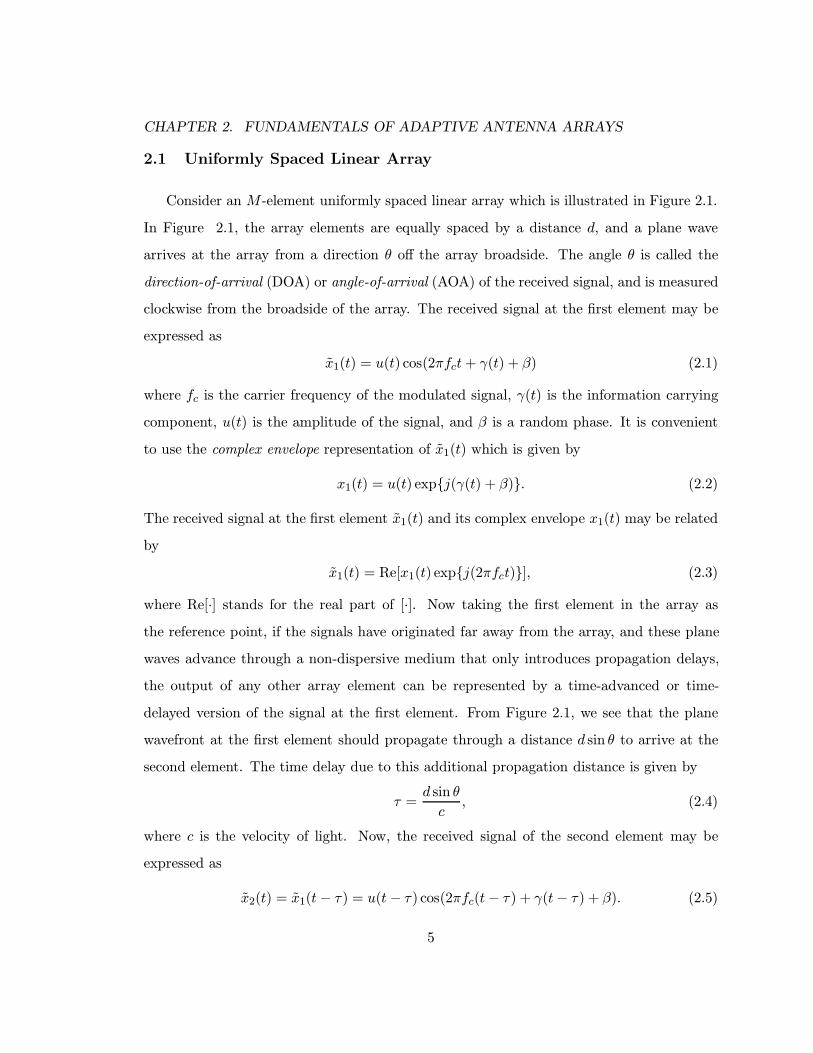
Consider an M -element uniformly spaced linear array which is illustrated in Figure 2.1.
In Figure 2.1, the array elements are equally spaced by a distance d, and a plane wave
arrives at the array from a direction θ off the array broadside. The angle θ is called the
direction-of-arrival (DOA) or angle-of-arrival (AOA) of the received signal, and is measured
clockwise from the broadside of the array. The received signal at the first element may be
expressed as
x1(t) = u(t) cos(2πfct+ γ(t) + β) (2.1)
where fc is the carrier frequency of the modulated signal, γ(t) is the information carrying
component, u(t) is the amplitude of the signal, and β is a random phase. It is convenient
to use the complex envelope representation of x1(t) which is given by
x1(t) = u(t) exp{j(γ(t) + β)}. (2.2)
The received signal at the first element x1(t) and its complex envelope x1(t) may be related
by
x1(t) = Re[x1(t) exp{j(2πfct)}], (2.3)
where Re[·] stands for the real part of [·]. Now taking the first element in the array as
the reference point, if the signals have originated far away from the array, and these plane
waves advance through a non-dispersive medium that only introduces propagation delays,
the output of any other array element can be represented by a time-advanced or time-
delayed version of the signal at the first element. From Figure 2.1, we see that the plane
wavefront at the first element should propagate through a distance d sin θ to arrive at the
second element. The time delay due to this additional propagation distance is given by
τ =d sin θ
c, (2.4)
where c is the velocity of light. Now, the received signal of the second element may be
expressed as
x2(t) = x1(t− τ) = u(t− τ) cos(2πfc(t− τ) + γ(t− τ) + β). (2.5)
5

CHAPTER 2. FUNDAMENTALS OF ADAPTIVE ANTENNA ARRAYS
d
12iM
θ
d θsin
Reference Element
PlaneWaveFront
IncidentPlane Wave
Figure 2.1: Illustration of a plane wave incident on a uniformly spaced linear array fromdirection θ.
If the carrier frequency fc is large compared to the bandwidth of the impinging signal, then
the modulating signal may be treated as quasi-static during time intervals of order τ and
in that case equation (2.5) reduces to
x2(t) = u(t) cos(2πfct− 2πfcτ + γ(t) + β). (2.6)
The complex envelope of x2(t) is therefore given by
x2(t) = u(t) exp{j(−2πfcτ + γ(t) + β)}
= x1(t) exp{−j(2πfcτ)}. (2.7)
From equation (2.7) we see that the effect of the time delay on the signal can now be
represented by a phase shift term exp{−j(2πfcτ)}. Substituting equation (2.4) into (2.7),
6
CHAPTER 2. FUNDAMENTALS OF ADAPTIVE ANTENNA ARRAYS
we have
x2(t) = x1(t) exp{−j(2πfcd sin θ
c)}
= x1(t) exp{−j(2π
λd sin θ)}, (2.8)
where λ is the wavelength of the carrier. In equation (2.8), we have used the relation
between c and fc, that is, fc = cλ . Similarly, for element i, the complex envelope of the
received signal may be expressed as
xi(t) = x1(t) exp{−j(2π
λ(i− 1)d sin θ)} i = 1, . . . ,M. (2.9)
Let
x(t) =
x1(t)
x2(t)...
xM (t)
(2.10)
and
a(θ) =
1
e−j2πλd sin θ
...
e−j2πλ
(M−1)d sin θ
(2.11)
then equation (2.9) may be expressed in vector form as
x(t) = a(θ)x1(t). (2.12)
The vector x(t) is often referred to as the array input data vector or the illumination vector,
and a(θ) is called the steering vector. The steering vector is also called direction vector, ar-
ray vector, array response vector, array manifold vector, DOA vector, or aperture vector. In
this case, the steering vector is only a function of the angle-of-arrival. In general, however,
the steering vector is also a function of the individual element response, the array geometry,
and signal frequency. The collection of steering vectors for all angles and frequencies is
7

CHAPTER 2. FUNDAMENTALS OF ADAPTIVE ANTENNA ARRAYS
referred to as the array manifold. Though for many simple arrays such as the uniformly
spaced linear array discussed above, the array manifold can be computed analytically, in
practice, the array manifold is measured as point source responses of the array at various an-
gles and frequencies. This process of obtaining the array manifold is called array calibration.
In the above discussion, the bandwidth of the impinging signal expressed in equa-
tion (2.9) is assumed to be much smaller than the reciprocal of the propagation time across
the array. Any signal satisfying this condition is referred to as narrowband, otherwise it is
referred to as wideband. In most of the discussion that follows, the signal is assumed to be
narrowband unless specified otherwise.
We could extend the above simple case to a more general case. Suppose there are q
narrowband signals s1(t), . . . , sq(t), all centered around a known frequency, say fc, impinging
on the array with a DOA θi, i = 1, 2, . . . , q. These signals may be uncorrelated, as for
the signals coming from different users, or can be fully correlated as happens in multipath
propagation, where each path is a scaled and time-delayed version of the original transmitted
signal, or can be partially correlated due to the noise corruption. The received signal at the
array is a superposition of all the impinging signals and noise. Therefore, the input data
vector may be expressed as
x(t) =q∑i=1
a(θi)si(t) + n(t), (2.13)
where
a(θi) =
1
e−j2πλd sin θi
...
e−j2πλ
(M−1)d sin θi
, (2.14)
and n(t) denotes the M × 1 vector of the noise at the array elements. In matrix notation,
equation (2.13) becomes
x(t) = A(Θ)s(t) + n(t) (2.15)
8

CHAPTER 2. FUNDAMENTALS OF ADAPTIVE ANTENNA ARRAYS
where A(Θ) is the M × q matrix of the steering vectors
A(Θ) = [a(θ1), . . . ,a(θq)] (2.16)
and
s(t) =
s1(t)
...
sq(t)
(2.17)
Equation (2.15) represents the most commonly used narrowband input data model.
Now let’s consider a special case. Assume that p users transmit signals from different
locations, and each user’s signal arrives at the array through multiple paths. Let LMi
denote the number of multipath components of the ith user. We have∑pi=1LMi = q. Let’s
further assume that all of the multipath components for a particular user arrive within a
time window which is much less than the channel symbol period for that user, then the
input data vector could be expressed as
x(t) =p∑i=1
LMi∑k=1
αi,ka(θi,k)si(t) + n(t)
=p∑i=1
bisi(t) + n(t), (2.18)
where θi,k is the DOA of the kth multipath component for the ith user, a(θi,k) is the steering
vector corresponding to θi,k, αi,k is the complex amplitude of the kth multipath component
for the ith user, and bi is the spatial signature for the ith user and is given by
bi =LMi∑k=1
αi,ka(θi,k) (2.19)
Similarly, equation (2.18) can be written in matrix form
x(t) = Bs(t) + n(t) (2.20)
where
B = [b1, . . . ,bp] (2.21)
9
CHAPTER 2. FUNDAMENTALS OF ADAPTIVE ANTENNA ARRAYS
and s(t) = [s1(t), . . . , sp(t)]T . The matrix B is called the spatial signature matrix.
In equation (2.15), if the data vector x(t) is sampled K times, at t1, . . . , tK , the sampled
data may be expressed as
X = A(Θ)S + N (2.22)
where X and N are the M ×K matrices containing K snapshots of the input data vector
and noise vector, respectively,
X = [x(t1), . . . ,x(tK)]
= [x(1), . . . ,x(K)] (2.23)
N = [n(t1), . . . ,n(tK)]
= [n(1), . . . ,n(K)] (2.24)
and S is the q ×K matrix containing K snapshots of the narrowband signals
S = [s(t1), . . . , s(tK)]
= [s(1), . . . , s(K)] . (2.25)
In equation (2.23), (2.24), and (2.25), we have replaced the time index ti with i, i = 1, . . . ,K,
for notational simplicity.
With the data model created above, most array processing problems may be categorized
as follows [6]. Given the sampled data X in a wireless system, determine:
1. the number of signals q
2. the DOAs θ1, . . . , θq
3. the signal waveforms s(1), . . . , s(K).
We shall refer to (1) as the detection problem, to (2) as the localization problem, and to (3)
as the beamforming problem, which is the focus of this research.
10

CHAPTER 2. FUNDAMENTALS OF ADAPTIVE ANTENNA ARRAYS
2.2 Beamforming and Spatial Filtering
Beamforming is one type of processing used to form beams to simultaneously receive
a signal radiating from a specific location and attenuate signals from other locations [7].
Systems designed to receive spatially propagating signals often encounter the presence of
interference signals. If the desired signal and interference occupy the same frequency band,
unless the signals are uncorrelated, e. g., CDMA signals, then temporal filtering often cannot
be used to separate signal from interference. However, the desired and interfering signals
usually originate from different spatial locations. This spatial separation can be exploited
to separate signal from interference using a spatial filter at the receiver. Implementing a
temporal filter requires processing of data collected over a temporal aperture. Similarly,
implementing a spatial filter requires processing of data collected over a spatial aperture.
A beamformer is a processor used in conjunction with an array of sensors (i. e., antenna
elements in an adaptive array) to provide a versatile form of spatial filtering. The sensor
array collects spatial samples of propagating wave fields, which are processed by the beam-
former. Typically a beamformer linearly combines the spatially sampled time series from
each sensor to obtain a scalar output time series in the same manner that an FIR filter lin-
early combines temporally sampled data. There are two types of beamformers, narrowband
beamformer, and wideband beamformer. A narrowband beamformer is shown in Figure 2.2.
In Figure 2.2, the output at time k, y(k), is given by a linear combination of the data at
the M sensors at time k:
y(k) =M∑i=1
w∗i xi(k), (2.26)
where ∗ denotes complex conjugate. Since we are now using the complex envelope repre-
sentation of the received signal, both xi(t) and wi are complex. The weight wi is called the
complex weight. The beamformer shown in Figure 2.2 is typically used for processing nar-
rowband signals. In the following discussion, each sensor is assumed to have all necessary
receiver electronics and A/D converters if beamforming is performed digitally.
11

CHAPTER 2. FUNDAMENTALS OF ADAPTIVE ANTENNA ARRAYS
w1∗
w2∗
wM∗
Σ
++
+
x1 k( )
x2 k( )
xM k( )
y k( )
Figure 2.2: A narrowband beamformer forms a linear combination of the sensor outputs.
Equation 2.26 may also be written in vector form as
y(k) = wHx(k) (2.27)
where
w =
w1
w2
...
wM
(2.28)
and H denotes the Hermitian (complex conjugate) transpose. The vector w is called the
complex weight vector.
12

CHAPTER 2. FUNDAMENTALS OF ADAPTIVE ANTENNA ARRAYS
Different from a narrowband beamformer, a wideband beamformer samples the prop-
agating wave field in both space and time and is often used when signals of significant
frequency extent (broadband) are of interest [7]. A wideband beamformer is shown in
Figure 2.3. The output in this case may be expressed as
y(k) =M∑i=1
K−1∑l=0
w∗i,lxi(k − l) (2.29)
where K − 1 is the number of delays in each of the M sensor channels. Let
w = [w1,0, . . . , w1,K−1, . . . , wM,0, . . . , wM,K−1]T (2.30)
and
x(k) = [x1(k), . . . , x1(k −K + 1), . . . , xM (k), . . . , xM (k −K + 1)]T , (2.31)
where T denotes the conventional transpose, equation (2.29) may also be expressed in vec-
tor form as in equation (2.27). In this case, both w and x(k) are MK × 1 column vectors.
Comparing Figure 2.2 with Figure 2.3, we see that a wideband beamformer is more
complex than narrowband beamformer. Since both types of beamformers may share the
same data model, we will concentrate on the narrowband beamformer in the following
discussion.
2.3 Beampattern and Element Spacing
The beampattern and element spacing of an antenna array may be viewed as the coun-
terpart of the magnitude response of a FIR filter and the sampling period of a discrete
time signal in the time domain, respectively. To illustrate this point, we may compare
the harmonic retrieval problem in the time domain with the beamforming problem in the
space domain [6]. Consider a signal x(t) composed of q complex sinusoids with unknown
13

CHAPTER 2. FUNDAMENTALS OF ADAPTIVE ANTENNA ARRAYS
Σ
x1 k( )
x2 k( )
xM k( )
y k( )
z-1 z-1
w1,0 w1,1 w1,K-1
z-1 z-1
w2,0 w2,1 w2,K-1
+
++
*
* **
* *
* * *
z-1 z-1
wM,0 wM,1 wM,K-1
Figure 2.3: A wideband beamformer samples the signal in both space and time.
14

CHAPTER 2. FUNDAMENTALS OF ADAPTIVE ANTENNA ARRAYS
parameters embedded in additive noise:
x(t) =q∑i=1
ai exp{j(2πfit+ φi)}+ n(t), (2.32)
where fi, ai, and φi are the frequency, amplitude, and phase, respectively, of the ith sinusoid.
Suppose that the signal is sampled with a sampling period Ts unrelated to the frequency of
the unknown sinusoid, and let x(l) denote the signal at time instant lTs, we have
x(l) =q∑i=1
ai exp{j(2πfi(lTs) + φi)}+ n(lTs). (2.33)
Suppose the sampled signal is fed into an FIR filter with M − 1 delay units, which is shown
in Figure 2.4, to perform filtering. At time instant lTs, the filter input and the M − 1
Σ
x l 1–( )
x l( )
x l M– 1+( )
y k( )
z-1
z-1
w1*
w2*
wM*
++
+
Figure 2.4: A FIR filter used to perform filtering in the time domain.
outputs of the delay units may be expressed as
x(l) =q∑i=1
a(fi)si(l) + n(l), (2.34)
15

CHAPTER 2. FUNDAMENTALS OF ADAPTIVE ANTENNA ARRAYS
where x(l) = [x(l), x(l − 1), . . . , x(l −M + 1)]T , n(l) = [n(lTs), . . . , n((l −M + 1)Ts)]T ,
a(fi) =
1
e−j2πTsfi
...
e−j2π(M−1)Tsfi
(2.35)
and
si(l) = ai exp{j(2πfi(lTs) + φi)}. (2.36)
Comparing equation (2.34), (2.35) with equation (2.13), (2.14), we see that for a narrow-
band uniform linear array (ULA), there is a correspondence between the normalized element
spacing, dλ , and the sampling period, Ts, in the FIR filter, also the sine of the DOA θi, sin θi,
can be related to the temporal frequency fi of the FIR filter input [7].
Since there is a mapping between the ULA and the FIR filter, a theorem applied to
the FIR filter in the time domain may also be applied to the uniform linear array in space
domain. In time domain, the Nyquist sampling theorem [8] stated that for a bandlimited
signal with highest frequency f , the signal is uniquely determined by its discrete time
samples if the sampling rate is equal to or greater than 2f . If the sampling rate is less than
2f , aliasing will occur. In the space domain, the sampling rate corresponds to the inverse
of the normalized element spacing, and the highest frequency is corresponding to 1 (since
sin θi is always less than 1). From the Nyquist sampling theorem, to avoid spatial aliasing,
we should have1dλ
≥ 2× 1 (2.37)
or equivalently,
d ≤ λ
2. (2.38)
Therefore, the element spacing of an array should always be less than or equal to half of the
carrier wavelength. However, the element spacing cannot be made arbitrarily small since
two closely spaced antenna elements will exhibit mutual coupling effects. It is difficult to
16

CHAPTER 2. FUNDAMENTALS OF ADAPTIVE ANTENNA ARRAYS
generalize these effects since they depend heavily on the type of antenna element and the
array geometry. However, the mutual coupling between two elements typically tends to in-
crease as the distance between elements is reduced [5]. Thus the spacing between elements
must be large enough to avoid significant mutual coupling. In a practical linear arrays, the
element spacing is often kept near a half wavelength so that the spatial aliasing is avoided
and the mutual coupling effect is minimized.
The frequency response of an FIR filter with tap weights w∗i , i = 1, . . . ,M and a sampling
period Ts is given by
H(ej2πf ) =M∑i=1
w∗i e−j2πfTs(i−1), (2.39)
where H(ej2πf ) represents the response of the filter to a complex sinusoid of frequency f .
For the harmonic retrieval problem, if we want to extract the signal with frequency fi,
we need to find a set of complex weights such that the frequency response of the filter
has a higher gain at fi and lower gains (or ideally, nulls) at other frequencies. For the
beamforming problem, since f and Ts are corresponding to sin θ and dλ , respectively, we can
replace f and Ts in equation (2.39) with sin θ and dλ , respectively, to get the beamformer
response,
g(θ) =M∑i=1
w∗i e−j 2π
λ(i−1)d sin θ, (2.40)
where g(θ) represents the response of the array to a signal with DOA equal to θ. So if there
are several signals coming from different directions, and we want to extract the signal with
direction θi, we need to find a set of weights such that the array response has a higher gain
at direction θi and lower gains (or ideally, nulls) at other directions.
The array response g(θ) may also be expressed in vector form as
g(θ) = wHa(θ), (2.41)
where w and a(θ) are defined in equation (2.28) and (2.14), respectively. The beamformer
response may also be viewed as the ratio of the beamformer output to the signal at the
17

CHAPTER 2. FUNDAMENTALS OF ADAPTIVE ANTENNA ARRAYS
reference element when a single plane wave is incident on the array.
The beampattern is defined as the magnitude of g(θ) [7] and is given by
G(θ) = |g(θ)|. (2.42)
Using G(θ), we may define the normalized beamformer response,
gn(θ) =g(θ)
max{G(θ)} (2.43)
where gn(θ) is also known as the normalized radiation pattern or array factor of the array.
The spatial discrimination capability of a beamformer depends on the size of the spatial
aperture of the array; as the aperture increases, discrimination improves. The absolute
aperture size is not important, rather its size in wavelengths is the critical parameter.
To illustrate this point, let us consider a uniform linear array with equal weight for each
element. From equation (2.40), we get the beamformer response
g(θ) =M∑i=1
e−j2πλ
(i−1)d sin θ
=1− e−j 2π
λMd sin θ
1− e−j 2πλd sin θ
(2.44)
=sin(πMd
λ sin θ)
sin(π dλ sin θ)e−jπ
(M−1)dλ
sin θ. (2.45)
The beampattern of this equal-weight beamformer is shown in Figure 2.5. The polar coor-
dinate plot of the beampattern is also shown in Figure 2.6. In Figure 2.5, the normalized
beampattern gain is expressed in dB. From equation (2.45), we see that the null-to-null
beamwidth, θBW , of the array is determined by
πMd
λsin θ = π. (2.46)
The solution of equation (2.46) may be expressed as
θH = arcsin
(λ
Md
)(2.47)
18

CHAPTER 2. FUNDAMENTALS OF ADAPTIVE ANTENNA ARRAYS
−80 −60 −40 −20 0 20 40 60 80−40
−35
−30
−25
−20
−15
−10
−5
0
DOA (degrees)
Bea
mpa
ttern
Gai
n (d
B)
Figure 2.5: Beampattern for an equal-weight beamformer. In this case, the number ofelements is equal to 8, and the element spacing is half of the carrier wavelength. The plotis generated by Programs [P1] and [P2].
0.2
0.4
0.6
0.8
1
60
−120
30
−150
0
180
−30
150
−60
120
−90 90
Figure 2.6: The same beampattern as shown in Figure 2.5 with polar coordinate plot inazimuth. The plot is generated by Programs [P1] and [P2].
19

CHAPTER 2. FUNDAMENTALS OF ADAPTIVE ANTENNA ARRAYS
where θH is the peak-to-null beamwidth, or half of the null-to-null beamwidth. The null-
to-null beamwidth is then obtained by
θBW = 2θH = 2 arcsin
(λ
Md
). (2.48)
From equation (2.48), we see that the beamwidth, which is the width of the main lobe
of the beampattern, is inversely proportional to the term Mdλ . Therefore, if the aperture
size in wavelengths is large, the beamwidth of the array will be small, and the beamformer
will have a high spatial discrimination capability. For a general beamformer with unequal
weights wiue, i = 1, 2, . . . ,M , the weight wiue may be viewed as the product of the equal
weight series and a periodic weight series:
wiue = wiewiue, i = −∞, . . . , 1, 2, . . . ,∞, (2.49)
where
wie =
1 i = 1, 2, . . . ,M
0 otherwise(2.50)
and
w(i+kM)ue = wiue, i = 1, 2, . . . ,M and k = −∞, . . . , 1, 2, . . . ,∞. (2.51)
Since in the time domain, the frequency response of a periodic time series contains a delta
function, similarly, in the space domain, the beampattern corresponding to the weight se-
ries wiue will have a high angle resolution. The resulting beampattern corresponding to the
unequal weight wiue thus can be viewed as the convolution of the equal-weight beampattern
with a beampattern having high angle resolution, and the beamwidth (or equivalently, the
aperture size in wavelength) of the equal-weight beamformer determines the spatial dis-
crimination capability of a general beamformer. So, in addition to minimizing the mutual
coupling effect between the array elements, maximizing the aperture size is another reason
to keep the element spacing of the array near a half wavelength.
From Figure 2.6, we see that the beampattern of the array is symmetrical about the axis
connecting the array elements. This symmetry of the beampattern is inherent in the uniform
20
CHAPTER 2. FUNDAMENTALS OF ADAPTIVE ANTENNA ARRAYS
linear array. From equation (2.40), we see that g(θ) = g(π − θ), thus the beampattern of
the uniform linear array is symmetrical about the endfire of the array. Arrays with non-
linear spacing or with other geometry, such as the circular array, do not exhibit this kind
of symmetry.
2.4 Adaptive Arrays
In a mobile communication system, the mobile is generally moving, therefore the DOAs
of the received signals in the base station are time-varying. Also, due to the time-varying
wireless channel between the mobile and the base station, and the existence of the cochannel
interference, multipath, and noise, the parameters of each impinging signal are varied with
time. For a beamformer with constant weights, the resulting beampattern cannot track
these time-varying factors. However, an adaptive array [9] may change its patterns auto-
matically in response to the signal environment. An adaptive array is an antenna system
that can modify its beampattern or other parameters, by means of internal feedback control
while the antenna system is operating. Adaptive arrays are also known as adaptive beam-
formers, or adaptive antennas. A simple narrowband adaptive array is shown in Figure 2.7.
In Figure 2.7, the complex weights w1, . . . , wM are adjusted by the adaptive control
processor. The method used by the adaptive control processor to change the weights is
called the adaptive algorithm. Most adaptive algorithms are derived by first creating a per-
formance criterion, and then generating a set of iterative equations to adjust the weights
such that the performance criterion is met. Some of the most frequently used performance
criteria include minimum mean squared error (MSE), maximum signal-to-interference-and-
noise ratio (SINR), maximum likelihood (ML), minimum noise variance, minimum output
power, maximum gain, etc. [9]. These criteria are often expressed as cost functions which
are typically inversely associated with the quality of the signal at the array output. As the
weights are iteratively adjusted, the cost function becomes smaller and smaller. When the
21

CHAPTER 2. FUNDAMENTALS OF ADAPTIVE ANTENNA ARRAYS
w1∗
w2∗
wM∗
Σ
++
+
x1 k( )
x2 k( )
xM k( )
y k( )
Adaptive Control Processor
.
.
.
.
Figure 2.7: A simple narrowband adaptive array.
cost function is minimized, the performance criterion is met and the algorithm is said to
have converged.
For one adaptive array, there may exist several adaptive algorithms that could be used
to adjust the weight vector. The choice of one algorithm over another is determined by
various factors [10]:
1. Rate of convergence. This is defined as the number of iterations required for the
algorithm, in response to stationary input, to converge to the optimum solution. A fast
22

CHAPTER 2. FUNDAMENTALS OF ADAPTIVE ANTENNA ARRAYS
rate of convergence allows the algorithm to adapt rapidly to a stationary environment
of unknown statistics.
2. Tracking. When an adaptive algorithm operates in a nonstationary environment, the
algorithm is required to track statistical variations in the environment.
3. Robustness. In one context, robustness refers to the ability of the algorithm to operate
satisfactorily with ill-conditioned input data. The term robustness is also used in the
context of numerical behavior.
4. Computational requirements. Here the issues of concern include (a) the number of
operations (i. e., multiplications, divisions, and additions/subtractions) required to
make one complete iteration of the algorithm, (b) the size of memory locations required
to store the data and the program, and (c) the investment required to program the
algorithm on a computer or a DSP processor.
Since there exists a mapping between the narrowband beamformer and the FIR filter, most
of the adaptive algorithms used by the adaptive filter [10] may be applied to the adaptive
beamformer. However, some of the adaptive beamforming algorithms also have their unique
aspects that an adaptive filter algorithm does not possess. A thorough survey of adaptive
beamforming algorithms is given in Chapter 3.
2.5 Summary
In this chapter we introduced terminology and basic concepts related to antenna array
and adaptive beamforming. The correspondence between a narrowband beamformer and a
FIR filter is also introduced. In Chapter 3, a survey of adaptive beamforming algorithms
is presented.
23

Chapter 3
Overview of Adaptive Beamforming Algorithms
3.1 Introduction
This chapter provides a thorough survey of adaptive beamforming algorithms. Most of
these algorithms may be categorized into two classes according to whether a training signal
is used or not. One class of these algorithms is the non-blind adaptive algorithm in which
a training signal is used to adjust the array weight vector. Another technique is to use a
blind adaptive algorithm which does not require a training signal.
Since the non-blind algorithms use a training signal, during the training period, data
cannot be sent over the radio channel. This reduces the spectral efficiency of the system.
Therefore, the blind algorithms are of more research interest. The research here focuses
primarily on blind beamforming algorithms.
3.2 Non-blind Adaptive Algorithms
In a non-blind adaptive algorithm, a training signal, d(t), which is known to both the
transmitter and receiver, is sent from the transmitter to the receiver during the training
period. The beamformer in the receiver uses the information of the training signal to
compute the optimal weight vector, wopt. After the training period, data is sent and the
beamformer uses the weight vector computed previously to process the received signal. If
the radio channel and the interference characteristics remain constant from one training
period until the next, the weight vector wopt will contain the information of the channel
and the interference, and their effect on the received signal will be compensated in the
24

CHAPTER 3. OVERVIEW OF ADAPTIVE BEAMFORMING ALGORITHMS
output of the array.
3.2.1 Wiener Solution
Most of the non-blind algorithms try to minimize the mean-squared error between the
desired signal d(t) and the array output y(t). Let y(k) and d(k) denote the sampled signal
of y(t) and d(t) at time instant tk, respectively. Then the error signal is given by [10]
e(k) = d(k) − y(k) (3.1)
and the mean-squared error is defined by
J = E[|e(k)|2], (3.2)
where E[·] denotes the ensemble expectation operator. Substituting equation (3.1) and
(2.27) into equation (3.2), we have
J = E[|d(k) − y(k)|2]
= E[{d(k) − y(k)}{d(k) − y(k)}∗]
= E[{d(k) −wHx(k)}{d(k) −wHx(k)}∗]
= E[|d(k)|2 − d(k)xH (k)w −wHx(k)d∗(k) + wHx(k)xH(k)w]
= E[|d(k)|2]− pHw−wHp + wHRw, (3.3)
where
R = E[x(k)xH (k)] (3.4)
and
p = E[x(k)d∗(k)]. (3.5)
In equation (3.3), R is the M×M correlation matrix of the input data vector x(k), and p is
the M×1 cross-correlation vector between the input data vector and the desired signal d(k).
25

CHAPTER 3. OVERVIEW OF ADAPTIVE BEAMFORMING ALGORITHMS
The gradient vector of J , ∇ (J), is defined by
∇ (J) = 2∂J
∂w∗, (3.6)
where ∂∂w∗ denotes the conjugate derivative with respect to the complex vector w (see
Appendix A for more details on differentiation with respect to a complex vector). When
the mean-squared error J is minimized, the gradient vector will be equal to a M × 1 null
vector.
∇ (J)∣∣wopt = 0 (3.7)
Substituting equation (3.3) into equation (3.7), we have
− 2p + 2Rwopt = 0 (3.8)
or equivalently
Rwopt = p. (3.9)
Equation (3.9) is called the Wiener-Hopf equation [10]. Premultiplying both sides of equa-
tion (3.9) by R−1, the inverse of the correlation matrix, we obtain
wopt = R−1p. (3.10)
The optimum weight vector wopt in equation (3.10) is called the Wiener solution. From
equation (3.10), we see that the computation of the optimum weight vector wopt requires
knowledge of two quantities: (1) the correlation matrix R of the input data vector x(k),
and (2) the cross-correlation vector p between the input data vector x(k) and the desired
signal d(k).
3.2.2 Method of Steepest-Descent
Although the Wiener-Hopf equation may be solved directly by calculating the product
of the inverse of the correlation matrix R and the cross-correlation vector p, nevertheless,
this procedure presents serious computational difficulties since calculating the inverse of the
26

CHAPTER 3. OVERVIEW OF ADAPTIVE BEAMFORMING ALGORITHMS
correlation matrix results in a high computational complexity. An alternative procedure is
to use the method of steepest-descent [10]. To find the optimum weight vector wopt by the
steepest-descent method we proceed as follows:
1. Begin with an initial value w(0) for the weight vector, which is chosen arbitrarily.
Typically, w(0) is set equal to a column vector of an M ×M identity matrix.
2. Using this initial or present guess, compute the gradient vector ∇ (J(k)) at time k
(i. e., the kth iteration).
3. Compute the next guess at the weight vector by making a change in the initial or
present guess in a direction opposite to that of the gradient vector.
4. Go back to step 2 and repeat the process.
It is intuitively reasonable that successive corrections to the weight vector in the direction
of the negative of the gradient vector should eventually lead to the minimum mean-squared
error Jmin, at which the weight vector assumes its optimum value wopt.
Let w(k) denote the value of the weight vector at time k. According to the method of
steepest-descent, the update value of the weight vector at time k + 1 is computed by using
the simple recursive relation
w(k + 1) = w(k) +1
2µ[−∇ (J(k))], (3.11)
where µ is a positive real-valued constant. The factor 12 is used merely for convenience.
From equation (3.8) we have
∇ (J(k)) = −2p + 2Rw(k). (3.12)
Substituting equation (3.12) into (3.11), we obtain
w(k + 1) = w(k) + µ[p−Rw(k)], k = 0, 1, 2, . . . . (3.13)
27

CHAPTER 3. OVERVIEW OF ADAPTIVE BEAMFORMING ALGORITHMS
Using equation (3.4), (3.5), (3.1), and (2.27), the gradient vector in equation (3.12) may be
written in another form
∇ (J(k)) = −2E[x(k)d∗(k)− x(k)xH (k)w(k)]
= −2E[x(k){d(k) − y(k)}∗]
= −2E[x(k)e∗(k)]. (3.14)
Also, equation (3.11) can be expressed as
w(k + 1) = w(k) + µE[x(k)e∗(k)]. (3.15)
We observe that the parameter µ controls the size of the incremental correction applied to
the weight vector as we proceed from one iteration cycle to the next. We therefore refer
to µ as the step-size parameter or weighting constant. Equations (3.13) and (3.15) describe
the mathematical formulation of the steepest-descent method.
3.2.3 Least-Mean-Squares Algorithm
If it were possible to make exact measurements of the gradient vector ∇ (J(k)) at each
iteration, and if the step-size parameter µ is suitably chosen, then the weight vector com-
puted by using the steepest-descent method would indeed converge to the optimum Wiener
solution. In reality, however, exact measurements of the gradient vector are not possible
since this would require prior knowledge of both the correlation matrix R of the input data
vector and the cross-correlation vector p between the input data vector and the desired sig-
nal. Consequently, the gradient vector must be estimated from the available data. In other
words, the weight vector is updated in accordance with an algorithm that adapts to the
incoming data. One such algorithm is the least-mean-squares (LMS) algorithm [10][11]. A
significant feature of the LMS algorithm is its simplicity; it does not require measurements
of the pertinent correlation functions, nor does it require matrix inversion.
28

CHAPTER 3. OVERVIEW OF ADAPTIVE BEAMFORMING ALGORITHMS
To develop an estimate of the gradient vector ∇ (J(k)), the most obvious strategy is to
substitute the expected value in equation (3.14) with the instantaneous estimate,
∇ (J(k)) = −2x(k)e∗(k). (3.16)
Substituting this instantaneous estimate of the gradient vector into equation (3.11), we have
w(k + 1) = w(k) + µx(k)e∗(k). (3.17)
Now, we can describe the LMS algorithm by the following three equations
y(k) = wH(k)x(k) (3.18)
e(k) = d(k)− y(k) (3.19)
w(k + 1) = w(k) + µx(k)e∗(k). (3.20)
The LMS algorithm is a member of a family of stochastic gradient algorithms since the
instantaneous estimate of the gradient vector is a random vector that depends on the input
data vector x(k). The LMS algorithm requires about 2M complex multiplications per
iteration, where M is the number of weights (elements) used in the adaptive array. The
response of the LMS algorithm is determined by three principal factors: (1) the step-size
parameter, (2) the number of weights, and (3) the eigen-value of the correlation matrix of
the input data vector. More details about the LMS algorithm are discussed in [10][12][13].
3.2.4 Recursive Least-Squares Algorithm
Unlike the LMS algorithm which uses the method of steepest-descent to update the
weight vector, the recursive least-squares (RLS) algorithm [10][12] uses the method of least
squares to adjust the weight vector. In the method of least squares, we choose the weight
vector w(k), so as to minimize a cost function that consists of the sum of error squares over
a time window. In the method of steepest-descent, on the other hand, we choose the weight
vector to minimize the ensemble average of the error squares.
29

CHAPTER 3. OVERVIEW OF ADAPTIVE BEAMFORMING ALGORITHMS
In the exponentially weighted RLS algorithm, at time k, the weight vector is chosen to
minimize the cost function
E(k) =k∑i=1
λk−i|e(i)|2 (3.21)
where e(i) is defined in equation (3.1), and λ is a positive constant close to, but less than,
one, which determines how quickly the previous data are de-emphasized. In a stationary
environment, however, λ should be equal to 1, since all data past and present should have
equal weight. The RLS algorithm is obtained from minimizing equation (3.21) by expanding
the magnitude squared and applying the matrix inversion lemma. The RLS algorithm can
be described by the following equations [10]
k(k) =λ−1P(k − 1)x(k)
1 + λ−1xH(k)P(k − 1)x(k)(3.22)
α(k) = d(k) −wH(k − 1)x(k) (3.23)
w(k) = w(k − 1) + k(k)α∗(k) (3.24)
P(k) = λ−1P(k − 1)− λ−1k(k)xH(k)P(k − 1). (3.25)
The initial value of P(k) can be set to
P(0) = δ−1I (3.26)
where I is the M ×M identity matrix, and δ is a small positive constant.
An important feature of the RLS algorithm is that it utilizes information contained
in the input data, extending back to the instant of time when the algorithm is initiated.
The resulting rate of convergence is therefore typically an order of magnitude faster than
the simple LMS algorithm. This improvement in performance, however, is achieved at
the expense of a large increase in computational complexity. The RLS algorithm requires
4M2 + 4M + 2 complex multiplications per iteration, where M is the number of weights
used in the adaptive array.
30

CHAPTER 3. OVERVIEW OF ADAPTIVE BEAMFORMING ALGORITHMS
3.3 Blind Adaptive Algorithms
Blind adaptive algorithms do not require a training sequence. Instead, they exploit
some known properties of the desired received signal. Most of the blind algorithms may be
categorized into the following three classes or combinations of them:
• Algorithms based on estimation of the DOAs of the received signals.
• Algorithms based on property-restoral techniques.
• Algorithms based on the discrete-alphabet structure of digital signals.
3.3.1 Algorithms Based on Estimation of DOAs of Received Signals
In the DOA-estimation-based algorithms, the DOAs of the received signals are first
determined by using prior knowledge of the array response, i. e., the array manifold or
special array structure. The high-resolution techniques for DOA estimation include MU-
SIC [14] and ESPRIT [15]. After the DOAs are estimated, an optimum beamformer is
then constructed from the corresponding array response to extract the desired signals from
interference and noise [16]. The performance of this technique strongly depends on the
reliability of the prior spatial information, e. g., the array manifold. In many situations of
practical interest, this information is not available. Even if this information is available,
the cost is very expensive and the information may be inaccurate. The computational com-
plexity of these algorithms is also very high. Another disadvantage of this technique is that
the number of DOAs that the algorithm can estimate is limited by the number of array
elements. In a wireless communication system, especially in a code division multiple access
(CDMA) system, the number of users in a radio channel may be greater than the number of
array elements, and if the multipaths of each user’s signal are taken into account, the total
number of signals impinging on the array will far exceed the number of array elements, and
the DOA estimation algorithm in this case will fail. Furthermore, this approach does not
exploit the known temporal structure of the incoming signals.
31
CHAPTER 3. OVERVIEW OF ADAPTIVE BEAMFORMING ALGORITHMS
3.3.2 Algorithms Based on Property-Restoral Techniques
Generally, most digital communication signals possess some kinds of properties such as
the constant modulus property or the spectral self-coherence property. Due to the inter-
ference, noise, and the time-varying channel in a communication system, these properties
may be corrupted when the signal is received at the receiver. The adaptive array in the re-
ceiver tries to restore these properties using a property-restoral-based algorithm, and hopes
that by restoring these properties, the output of the array is a reconstructed version of the
transmitted signal.
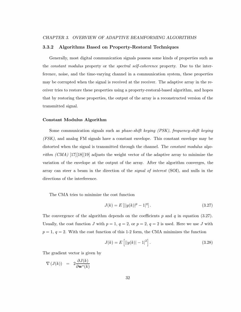
Constant Modulus Algorithm
Some communication signals such as phase-shift keying (PSK), frequency-shift keying
(FSK), and analog FM signals have a constant envelope. This constant envelope may be
distorted when the signal is transmitted through the channel. The constant modulus algo-
rithm (CMA) [17][18][19] adjusts the weight vector of the adaptive array to minimize the
variation of the envelope at the output of the array. After the algorithm converges, the
array can steer a beam in the direction of the signal of interest (SOI), and nulls in the
directions of the interference.
The CMA tries to minimize the cost function
J(k) = E [||y(k)|p − 1|q] . (3.27)
The convergence of the algorithm depends on the coefficients p and q in equation (3.27).
Usually, the cost function J with p = 1, q = 2, or p = 2, q = 2 is used. Here we use J with
p = 1, q = 2. With the cost function of this 1-2 form, the CMA minimizes the function
J(k) = E[||y(k)| − 1|2
]. (3.28)
The gradient vector is given by
∇ (J(k)) = 2∂J(k)
∂w∗(k)
32

CHAPTER 3. OVERVIEW OF ADAPTIVE BEAMFORMING ALGORITHMS
= 2E
[(|y(k)| − 1)
∂|y(k)|∂w∗(k)
]
= 2E
(|y(k)| − 1)∂ {y(k)y∗(k)}
12
∂w∗(k)
= 2E
(|y(k)| − 1)∂{wH(k)x(k)xH (k)w(k)
} 12
∂w∗(k)
= E
(|y(k)| − 1){wH(k)x(k)xH (k)w(k)
}− 12∂{wH(k)x(k)xH (k)w(k)
}∂w∗(k)
= E
[(|y(k)| − 1)
1
|y(k)|x(k)xH (k)w(k)
]= E
[(1− 1
|y(k)|
)x(k)y∗(k)
]= E
[x(k)
(y(k)− y(k)
|y(k)|
)∗]. (3.29)
Ignoring the expectation operator in equation (3.29), the instantaneous estimate of the
gradient vector can be written as
∇ (J(k)) = x(k)
(y(k)− y(k)
|y(k)|
)∗. (3.30)
Using the method of steepest-descent, and replacing the gradient vector with its instanta-
neous estimate, we can update the weight vector by
w(k + 1) = w(k)− µ∇ (J(k))
= w(k)− µx(k)
(y(k)− y(k)
|y(k)|
)∗(3.31)
where µ is the step-size parameter. Now, we can describe the steepest-descent CMA (SD-
CMA) by the following three equations
y(k) = wH(k)x(k) (3.32)
e(k) = y(k)− y(k)
|y(k)| (3.33)
w(k + 1) = w(k)− µx(k)e∗(k). (3.34)
33

CHAPTER 3. OVERVIEW OF ADAPTIVE BEAMFORMING ALGORITHMS
From equation (3.33) we see that when the output of the array has a unity magnitude,
i. e., |y(k)| = 1, the error signal becomes zero. Comparing the above three equations with
equation (3.18), (3.19), and (3.20), we see that the CMA is very similar to the LMS al-
gorithm, and the term y(k)|y(k)| in CMA plays the same role as the desired signal d(t) in the
LMS algorithm. However, the reference signal d(t) must be sent from the transmitter to
the receiver and must be known for both the transmitter and receiver if the LMS algorithm
is used. The CMA algorithm does not require a reference signal to generate the error signal
at the receiver.
Several properties of the constant modulus algorithm are discussed in [17]. One of the
properties is the phase roll or phase ambiguity. In CMA, if a weight vector w generates an
array output with constant modulus, so does its phase shifted version,
wr = ejφw. (3.35)
In other words, the phase of the array output, y(k), is indeterminate, which is in contrast
to the LMS algorithm. This is reasonable, since CMA uses only the amplitude information
of the array output in the control of the system and the phase information is not utilized.
The convergence behavior of CMA is discussed in [20][21][22][23]. It was found that the
constant modulus cost function will in general have two classes of stationary solutions in
the single signal-of-interest (SOI) environment: signal-capture solutions where the signal
is captured with maximum attainable signal-to-interference-and-noise ratio (SINR), and
noise-capture solutions where the desired signal is nulled by the array. The noise-capture
solutions must be avoided if the array is being used to extract the signal of interest.
Least-Squares CMA The constant modulus algorithm was first used by Gooch [24] in
the beamforming problem. After that, many CMA-type algorithms have been proposed
for use in adaptive arrays. In [25], B. G. Agee developed the least-squares constant mod-
ulus algorithm (LS-CMA) by using the extension of the method of nonlinear least-squares
34

CHAPTER 3. OVERVIEW OF ADAPTIVE BEAMFORMING ALGORITHMS
(Gauss’s method) [26]. The extension of Gauss’s method states that if a cost function can
be expressed in the form
F (w) =K∑k=1
|gk(w)|2
= ‖g(w)‖22, (3.36)
where
g(w) = [g1(w), g2(w), . . . , gK(w)]T , (3.37)
then the cost function has a partial Taylor-series expansion with sum-of-squares form
F (w + ∆) ≈∥∥∥g(w) + DH(w)∆
∥∥∥2
2, (3.38)
where ∆ is an offset vector, and
D(w) = [∇ (g1(w)) ,∇ (g2(w)) , . . . ,∇ (gK(w))] (3.39)
The gradient vector of F (w + ∆) with respect to ∆ is given by
∇∆(F (w + ∆)) = 2∂F (w + ∆)
∂∆∗
= 2∂{g(w) + DH(w)∆
}H {g(w) + DH(w)∆
}∂∆∗
= 2∂{‖g(w)‖22 + gH(w)DH(w)∆ + ∆HD(w)g(w) + ∆HD(w)DH(w)∆
}∂∆∗
= 2{D(w)g(w) + D(w)DH (w)∆
}. (3.40)
Setting ∇∆(F (w + ∆)) equal to zero, we can find the offset vector which minimizes
F (w + ∆),
∆ = −[D(w)DH(w)
]−1D(w)g(w). (3.41)
Therefore, the weight vector can be updated by
w(l + 1) = w(l)−[D(w(l))DH (w(l))
]−1D(w(l))g(w(l)) (3.42)
35

CHAPTER 3. OVERVIEW OF ADAPTIVE BEAMFORMING ALGORITHMS
where l denotes the iteration number. The LS-CMA is derived by applying equation (3.42)
to the constant modulus cost function,
F (w) =K∑k=1
||y(k)| − 1|2
=K∑k=1
∣∣∣|wHx(k)| − 1∣∣∣2 . (3.43)
Comparing equation (3.43) with (3.36), we see that in this case,
gk(w) = |y(k)| − 1
= |wHx(k)| − 1. (3.44)
Substituting equation (3.44) into (3.37), we obtain
g(w) =
|y(1)| − 1
|y(2)| − 1...
|y(K)| − 1
. (3.45)
The gradient vector of gk(w) is given by
∇ (gk(w)) = 2∂gk(w)
∂w∗
= x(k)y∗(k)
|y(k)| . (3.46)
Substituting equation (3.46) into (3.39), D(w) can be expressed as
D(w) = [∇ (g1(w)) ,∇ (g2(w)) , . . . ,∇ (gK(w))]
=
[x(1)
y∗(1)
|y(1)| ,x(2)y∗(2)
|y(2)| , . . . ,x(K)y∗(K)
|y(K)|
]= XYCM , (3.47)
where
X = [x(1),x(2), . . . ,x(K)] (3.48)
36
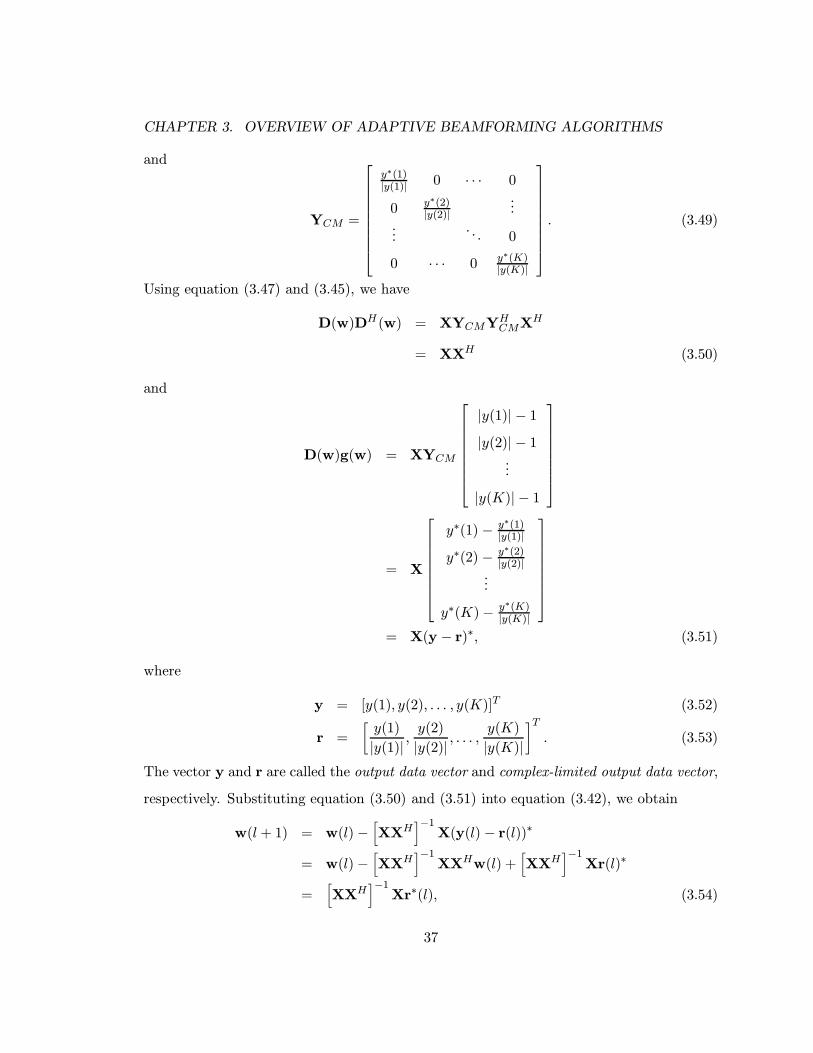
CHAPTER 3. OVERVIEW OF ADAPTIVE BEAMFORMING ALGORITHMS
and
YCM =
y∗(1)|y(1)| 0 · · · 0
0 y∗(2)|y(2)|
......
. . . 0
0 · · · 0 y∗(K)|y(K)|
. (3.49)
Using equation (3.47) and (3.45), we have
D(w)DH (w) = XYCMYHCMXH
= XXH (3.50)
and
D(w)g(w) = XYCM
|y(1)| − 1
|y(2)| − 1...
|y(K)| − 1
= X
y∗(1) − y∗(1)|y(1)|
y∗(2) − y∗(2)|y(2)|
...
y∗(K)− y∗(K)|y(K)|
= X(y − r)∗, (3.51)
where
y = [y(1), y(2), . . . , y(K)]T (3.52)
r =
[y(1)
|y(1)| ,y(2)
|y(2)| , . . . ,y(K)
|y(K)|
]T. (3.53)
The vector y and r are called the output data vector and complex-limited output data vector,
respectively. Substituting equation (3.50) and (3.51) into equation (3.42), we obtain
w(l + 1) = w(l)−[XXH
]−1X(y(l) − r(l))∗
= w(l)−[XXH
]−1XXHw(l) +
[XXH
]−1Xr(l)∗
=[XXH
]−1Xr∗(l), (3.54)
37

CHAPTER 3. OVERVIEW OF ADAPTIVE BEAMFORMING ALGORITHMS
where y(l) and r(l) are the output data vector and complex-limited output data vector
corresponding to the weight vector w(l) in the lth iteration, respectively.
The LS-CMA can be implemented both statically or dynamically. The static LS-CMA
repeatedly uses one data block X, which contains K snapshots of the input data vectors,
in the updating of the weight vector w. In the static LS-CMA, after a new weight vector
w(l + 1) is calculated using equation (3.54), this new weight vector is used with the input
data block X, which was also used in the last iteration, to generate the new output data
vector y(l+1) and the complex-limited output data vector r(l+1). The new complex-limited
output data vector is then substituted into equation (3.54) to generate a new weight vector.
In dynamic LS-CMA, however, different input data blocks are used during the updating of
the weight vector. Let X(l) denote the input data block used in the the lth iteration. X(l)
can be expressed as
X(l) = [x(1 + lK),x(2 + lK), . . . ,x((l + 1)K)] , l = 0, 1, . . . , L, (3.55)
where L is the number of iterations required for the algorithm to converge. Using X(l), we
can describe the dynamic LS-CMA by the following equations
y(l) =[wH(l)X(l)
]T= [y(1 + lK), y(2 + lK), . . . , y((l + 1)K)]T (3.56)
r(l) =
[y(1 + lK)
|y(1 + lK)| ,y(2 + lK)
|y(2 + lK)| , . . . ,y((l + 1)K)
|y((l + 1)K)|
]T(3.57)
w(l + 1) =[X(l)XH(l)
]−1X(l)r∗(l). (3.58)
From the above equations we see that while the SD-CMA updates the weight vector on
a sample-by-sample basis, the dynamic LS-CMA adjusts the weight vector on a block-by-
block basis. Since the LS-CMA can exploit the information in a data block, it converges
faster than the SD-CMA algorithm.
38

CHAPTER 3. OVERVIEW OF ADAPTIVE BEAMFORMING ALGORITHMS
If we define
Rxx(l) =1
KX(l)XH(l) (3.59)
pxr(l) =1
KX(l)r∗(l), (3.60)
equation (3.58) can also be written as
w(l + 1) = R−1xx (l)pxr(l). (3.61)
Some may find that equation (3.61) is very similar to (3.10), however, in equation (3.61),
Rxx(l) is an estimate of the correlation matrix of the input data vector, computed over the
lth data block containing K snapshots of the input data vector, and pxr(l) is an estimate
of the cross-correlation between the input data vector and the complex-limited output signal.
In [27], B. G. Agee applied the dynamic LS-CMA to a multitarget problem and developed
the multitarget least-squares constant modulus algorithm (MT-LSCMA). The challenge of
the multitarget problem is to separate and extract the signals if all the signals in the
communication system have the same constant modulus property. We will discuss the
MT-LSCMA in greater detail in Chapter 4.
Other CMA-type Algorithms In addition to the LS-CMA, many CMA-type beam-
forming algorithms have been proposed in the literature. In [28], Rude and Griffiths try
to incorporate the signal or environment information, such as the direction of arrival or
carrier frequency of the SOI, into the CMA algorithm. They transfer the a priori knowl-
edge of the signal into a set of linear constraints on the weight vector and developed the
linearly-constrained CMA. In [29], Fujimoto et al. used the Marquardt method, which is a
combination of Gauss’s method and the steepest-descent method, in the updating of the
weight vector. It was reported that the algorithm using Marquardt’s method converges
faster than the steepest-descent method.
39
CHAPTER 3. OVERVIEW OF ADAPTIVE BEAMFORMING ALGORITHMS
In [30], Shynk and Gooch proposed the multistage CMA beamformer to separate mul-
tiple narrowband signals. The multistage CMA beamformer is comprised of a cascade of
CM array subsections, each of which captures one of the signals impinging on the array. An
adaptive signal canceler follows each CM array to remove captured signals from the input
before processing by subsequent sections. However, it was reported in [31] that the capture
performance of the cascade CM array gradually deteriorates with increasing source cross-
correlation. To overcome this loss, Mathur et al. proposed a parallel version of the multistage
CM array that is appropriately initialized by a direction-finding algorithm. The combina-
tion of CMA with MUSIC in the parallel multistage CMA beamformer was reported in [32].
In [24], Gooch developed the orthogonalized-CMA (O-CMA) by multiplying the correc-
tion term (the scaled instantaneous estimate of the gradient vector) of the original CMA by
the inverse of the correlation matrix of the input data vector. This multiplication represents
an orthogonalization process of the correlation matrix of the received data which results in
reduction of the number of iterations required for convergence at the expense of some added
mathematical complexity. In [33], Pickholtz and Elbarbary proposed the recursive CMA
(R-CMA) which is based on the analogy to the RLS as a speeded-up version of the LMS.
Like RLS, R-CMA uses a cost function which is the sum of the exponentially weighted
squared error over a time window. It was reported in [33] that the R-CMA converges one
order of magnitude faster than the original CMA. The R-CMA could be viewed as a gen-
eralized version of the O-CMA.
In [34], Parra et al. developed the iterative least-squares with projection constant mod-
ulus algorithm (ILSP-CMA). Different from the algorithms discussed above, ILSP-CMA
does not update the weight vector, instead, it estimates the steering matrix A and the
narrowband signal data matrix S in equation (2.22) directly by using the iterative least-
squares with projection method. The ILSP-CMA tries to minimize the cost function
J(A,S) =‖ X−AS ‖2F and can be described as follows:
40

CHAPTER 3. OVERVIEW OF ADAPTIVE BEAMFORMING ALGORITHMS
1. Given A(0), l = 0
2. l = l + 1
• S(l) =(AH(l − 1)A(l − 1)
)−1AH(l − 1)X
• Project the (i, j) element of S(l) to the closest value on the unit circle
• A(l) = XSH(l)(S(l)SH(l)
)−1
3. Iterate again until A(l) and A(l − 1) are close enough or the distance between them
is below the preset threshold.
It was reported in [34] that the ILSP-CMA can separate multiple sources for low-to-high
signal-to-noise ratio (SNR) even when they have equal power. It was also reported that the
ILSP-CMA can converge very fast. However, to use ILSP-CMA, we need to first determine
the number of signals impinging on the array, which is very difficult for a CDMA system
with multipath for each user.
All the beamformer adaptation algorithms discussed to date are performed in data space
(element space). The adaptation process can also be performed in beam space. In [35],
Chiba et al. proposed the beam-space CMA (BS-CMA). In the BS-CMA, a multibeam is
formed by means of a fast Fourier transform (FFT) and only the beams whose output
power exceeds a threshold level are selected. The CMA is then used on the selected beam
outputs to perform the adaptation process. It was reported in [35] that the BS-CMA has
an advantage of carrying out the capture of the desired signal and the elimination of the
interference effectively with degrees of freedom corresponding to the number of impinging
signals. Hence, this algorithm is effective for applications to adaptive arrays with a relatively
large number of elements (more than 10) used in mobile satellite communications. It was
also reported in [35] that the BS-CMA converges faster than the conventional element-space
CMA (ES-CMA) and can increase the dynamic range of the received signal power. In [36],
Chiba el al. used the BS-CMA for null beam forming in the transmitting.
41

CHAPTER 3. OVERVIEW OF ADAPTIVE BEAMFORMING ALGORITHMS
Spectral Self-Coherence Restoral Algorithm
Most communication signals exhibit a property called cyclostationarity which can be ex-
ploited to achieve blind adaptive beamforming. Cyclostationarity is a term used to describe
the repetitive or cyclic nature of the statistics associated with communication signals [37].
Periodicities in the second order statistics of a signal lead to the existence of a correlation
between the signal and the frequency-shifted and possibly conjugated versions of itself for
certain discrete values of frequency shift. This property is called spectral self-coherence
or spectral conjugate self-coherence [38]. The cyclic correlation function and the cyclic
conjugate-correlation function of a signal s(t) are defined by
Rαss(τ)4=
⟨s(t+
τ
2)s∗(t− τ
2)e−j2παt
⟩∞
(3.62)
Rαss∗(τ)4=
⟨s(t+
τ
2)s(t− τ
2)e−j2παt
⟩∞, (3.63)
where 〈·〉 denotes the time averaging operator,
〈·〉 4= limT→∞
1
T
∫ T2
−T2
(·) dt (3.64)
and τ and α denote the time delay and frequency shift, respectively. Most communication
signals exhibit spectral correlation at one or more cycle frequencies (the doubled carrier
frequency or the baud rate or chip rate, etc.).
Based on the cyclic correlation function and the cyclic conjugate-correlation function,
Agee et al. developed a class of the spectral self-coherence restoral (SCORE) algorithms [38].
In [38], three SCORE algorithms: the least-squares SCORE, cross-SCORE, and auto-
SCORE algorithms, are proposed. However, these algorithms cannot separate multiple
signals having the same cyclic feature, which is just the case in a CDMA system. Some
variations of the SCORE algorithms are proposed by Biedka in [39][40] to increase the con-
vergence speed and reduce the computational complexity of the SCORE algorithm. In [41],
Castedo et al. proposed a new algorithm using a new cost function, J =⟨∣∣ej2παt − yp(t)∣∣2⟩.
42

CHAPTER 3. OVERVIEW OF ADAPTIVE BEAMFORMING ALGORITHMS
In [42], they analyzed the behavior of this algorithm in a multipath environment and re-
ported that this algorithm behaves like the CM beamformer in multipath environments but
overcomes the capture limitation of CM beamformers.
3.3.3 Algorithms Based on Discrete-Alphabet Structure of Digital Signal
This type of algorithm exploits the discrete-alphabet property of digitally modulated
signals to provide unique signal estimates. Similar to ILSP-CMA, this type of algorithm
tries to minimize the cost function J(A,S) =‖ X−AS ‖2F , where the elements of S are
constrained to a finite alphabet. In [43], Talwar et al. proposed three algorithms: the
iterative least squares with projection (ILSP) algorithm, the iterative least squares with
enumeration (ILSE) algorithm, and the recursive least squares with enumeration (RLSE)
algorithm. The performance of these algorithms is analyzed in [44]. However, all the
above three algorithms were developed under the assumption that all of the signals arrive
synchronously at the array, which is not necessarily true in reality.
3.3.4 Other Blind Beamforming Algorithms
In addition to the three classes of blind beamforming algorithms discussed above, there
are other blind algorithms that are reported in the literature.
2D RAKE Receiver
A RAKE receiver in a CDMA system combines the multipath components of a signal
to improve the system performance [45][46]. However, if the delay between the multipath
components is less than the chip period, the components cannot be resolved and the con-
ventional RAKE receiver will fail. In [47][48], Suard et al. proposed the 2D RAKE receiver
exploiting the spatial property of each multipath components such that the components
with time delay less than the chip period but with different DOAs can still be resolved
and optimumly combined. The 2D RAKE receiver estimates the pre-processing (before
43

CHAPTER 3. OVERVIEW OF ADAPTIVE BEAMFORMING ALGORITHMS
matched filtering) and post-processing array correlation matrices. The appropriately con-
structed differences of these estimates are then used to estimate the steering vector and
the noise covariance matrix, which are then used to get the beamforming weight vectors.
The system capacity improvement obtained by using the 2D RAKE receiver is analyzed
in [49][50]. However, the 2D RAKE receiver tries to steer one beam to each multipath
component of each user, which will result in a high computational complexity and highly
complicated hardware construction.
Decision Directed Algorithms
In a communication system with low bit error rate (BER), the demodulated signal can
be used as the reference signal in the adaptation of the weight vector. Such a method of
adaptation is said to be decision directed (DD), because the beamformer attempts to adapt
by employing its own decisions. The DD algorithm was first used in the adaptive equal-
ization problem [51]. If the BER is small, the decisions made by the receiver are correct
enough for the estimate of the error signal to be accurate most of the time. This means
that, in general, the adaptive beamformer is able to improve the weight vector by virtue of
the correlation procedure built into its feedback control loop. The improved weight vector
will, in turn, result in a lower BER and therefore more accurate estimates of the error signal
for adaptation, and so on. However, it is also possible for the reverse effect to occur, in
which case the weight vector loses acquisition of the channel.
For a BPSK signal, the adaptation equations for steepest-descent DD (SD-DD) algorithm
can be obtained by replacing the complex limited signal y(k)|y(k)| in the SD-CMA by the
decision term sgn[Re(y(k))], where sgn(·) denotes the signum function. Therefore, the SD-
DD algorithm can be described by the following equations
y(k) = wH(k)x(k) (3.65)
e(k) = y(k)− sgn[Re(y(k))] (3.66)
44

CHAPTER 3. OVERVIEW OF ADAPTIVE BEAMFORMING ALGORITHMS
w(k + 1) = w(k)− µx(k)e∗(k). (3.67)
In [52], Hilal et al. proposed an algorithm that allows soft transition between the CMA
and the DD algorithm for PSK modulated signals. This algorithm was shown to have the
robustness of the CMA behavior at the beginning of the convergence phase, and the precision
of the DD behavior near the convergence position. For a BPSK signal, this algorithm is
exactly the same as the SD-DD algorithm. The SD-DD algorithm can also be applied to
the multitarget problem. The multitarget steepest-descent decision directed (MT-SDDD)
algorithm will be discussed in detail in Chapter 4.
Others
Other beamforming algorithms for antenna arrays used in a CDMA system include one
proposed by Kohno et al. in [53], and one proposed by Jones et al. in [54]. In [53], Kohno et
al. proposed a scheme that adaptively estimates the multiple access interference from the
desired signal, which is then used to generate a reference signal for the adaptive null-steering
front end. They proposed two structures for the interference cancelation: serial and parallel.
In [54], Jones et al. investigated the use of an adaptive antenna array to null interference
in spread-spectrum receiver when the approximate position of the transmitter is known.
It was reported that incomplete directional knowledge may be exploited to enhance signal
equality and speed up code acquisition.
3.4 Summary
In this chapter we present an overview of the adaptive beamforming algorithms. Both
the non-blind and blind algorithms are described. In Chapter 4, we will give a detailed
description of the algorithms used in this research, which include a family of novel algorithms
developed in this research.
45

Chapter 4
Adaptive Beamforming Algorithms Used inSimulation
4.1 Introduction
In Chapter 3, we give a thorough survey of adaptive beamforming algorithms. In this
chapter, we will describe the algorithms used in this research in detail. Our research will
focus on the blind adaptive beamformer used in the base station in a CDMA system.
Since in a CDMA system, multiple users share a radio channel, our adaptive beamforming
algorithms should have the ability to separate and extract each user’s signal blindly and
simultaneously, in other words, the algorithms should be multitarget-type blind algorithms.
In this chapter, we will present four algorithms
• multitarget least-squares constant modulus algorithm (MT-LSCMA)
• multitarget decision-directed (MT-DD) algorithm
• least-squares despread respread multitarget array (LS-DRMTA)
• least-squares despread respread multitarget constant modulus algorithm (LS-DRMTCMA)
The LS-DRMTA and LS-DRMTCMA are two new algorithms developed in this research.
4.2 Multitarget Beamformer
In a CDMA mobile communication system, multiple users occupy the same frequency
band. The beamformer in the base station attempts to form a beam directed to each user
such that for one desired user, the interference from other directions is reduced. For a
46
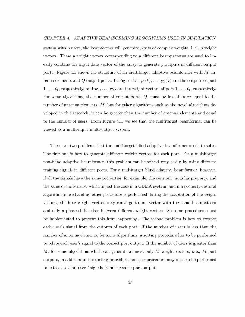
CHAPTER 4. ADAPTIVE BEAMFORMING ALGORITHMS USED IN SIMULATION
system with p users, the beamformer will generate p sets of complex weights, i. e., p weight
vectors. These p weight vectors corresponding to p different beampatterns are used to lin-
early combine the input data vector of the array to generate p outputs in different output
ports. Figure 4.1 shows the structure of an multitarget adaptive beamformer with M an-
tenna elements and Q output ports. In Figure 4.1, y1(k), . . . , yQ(k) are the outputs of port
1, . . . , Q, respectively, and w1, . . . ,wQ are the weight vectors of port 1, . . . , Q, respectively.
For some algorithms, the number of output ports, Q, must be less than or equal to the
number of antenna elements, M , but for other algorithms such as the novel algorithms de-
veloped in this research, it can be greater than the number of antenna elements and equal
to the number of users. From Figure 4.1, we see that the multitarget beamformer can be
viewed as a multi-input multi-output system.
There are two problems that the multitarget blind adaptive beamformer needs to solve.
The first one is how to generate different weight vectors for each port. For a multitarget
non-blind adaptive beamformer, this problem can be solved very easily by using different
training signals in different ports. For a multitarget blind adaptive beamformer, however,
if all the signals have the same properties, for example, the constant modulus property, and
the same cyclic feature, which is just the case in a CDMA system, and if a property-restoral
algorithm is used and no other procedure is performed during the adaptation of the weight
vectors, all these weight vectors may converge to one vector with the same beampattern
and only a phase shift exists between different weight vectors. So some procedures must
be implemented to prevent this from happening. The second problem is how to extract
each user’s signal from the outputs of each port. If the number of users is less than the
number of antenna elements, for some algorithms, a sorting procedure has to be performed
to relate each user’s signal to the correct port output. If the number of users is greater than
M , for some algorithms which can generate at most only M weight vectors, i. e., M port
outputs, in addition to the sorting procedure, another procedure may need to be performed
to extract several users’ signals from the same port output.
47
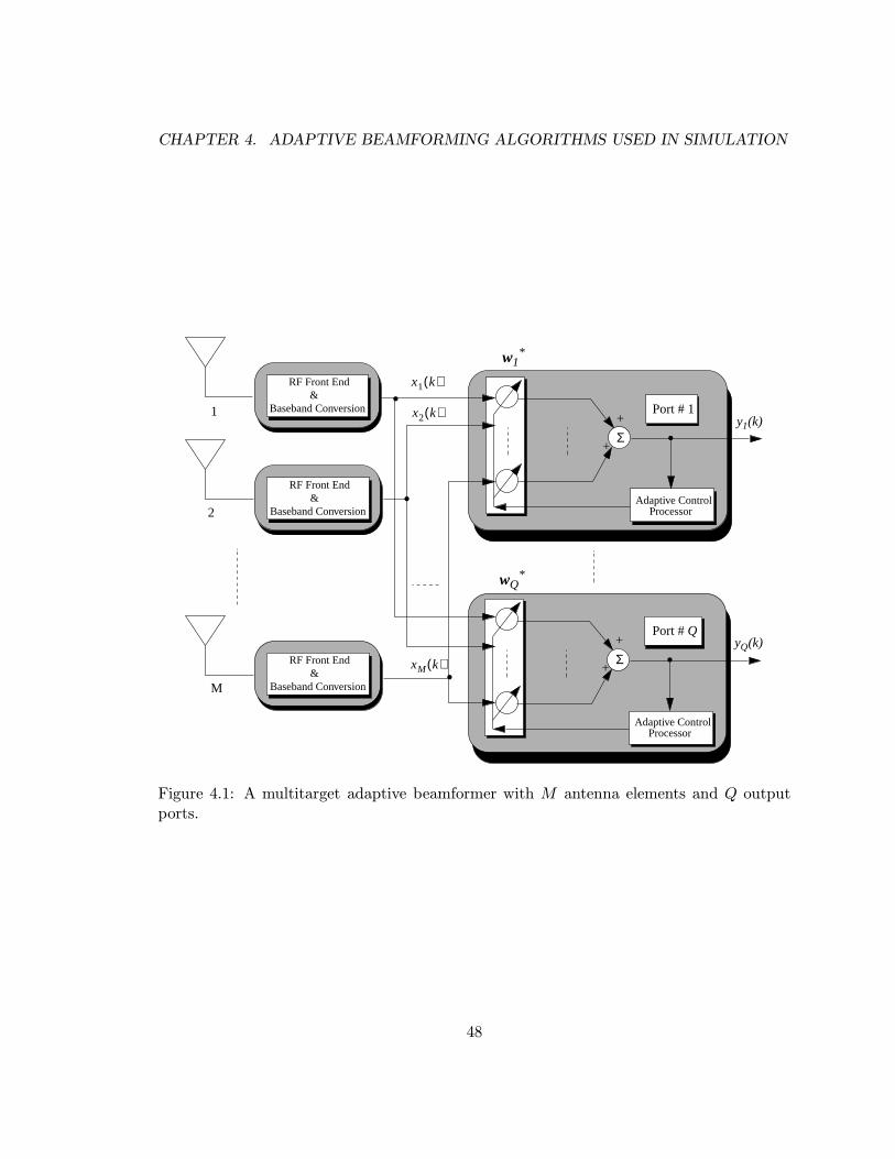
CHAPTER 4. ADAPTIVE BEAMFORMING ALGORITHMS USED IN SIMULATION
RF Front End&
Baseband Conversion
RF Front End&
Baseband Conversion
RF Front End&
Baseband Conversion
Σ
Adaptive Control Processor
+
+.
Port # 1
Σ
Adaptive Control Processor
+
+.
Port #Q
y1(k)
yQ(k)
1
M
x1 k( )
2
x2 k( )
xM k( )
w1*
wQ*
.
.
.
Figure 4.1: A multitarget adaptive beamformer with M antenna elements and Q outputports.
48

CHAPTER 4. ADAPTIVE BEAMFORMING ALGORITHMS USED IN SIMULATION
4.3 Multitarget Least-Squares Constant Modulus Algorithm
The multitarget least-squares constant modulus algorithm (MT-LSCMA) was first pro-
posed by Agee in [27]. This algorithm contains three principle components: a soft-orthogonalized
dynamic LS-CMA, a set of sorting and classification algorithms, and a fast acquisition al-
gorithm. However, the MT-LSCMA in [27] requires a high computational complexity. Here
we modify the original algorithm to reduce the computational complexity.
Figure 4.2 shows the structure of a MT-LSCMA adaptive array. In Figure 4.2, the
number of output ports is equal to the number of antenna elements, and the weight vectors
w1, . . . ,wM are initialized with a set of different vectors, for example, the column vectors of
a M×M identity matrix. These vectors are then adapted independently by the dynamic LS-
CMA which is described by equation (3.56), (3.57), and (3.58). However, since the LS-CMA
only utilizes the a priori information that the original signals have a constant envelope, for
a CDMA system with all the transmitted signals having the constant modulus property, if
there is no procedure implemented, all the weight vectors in different ports may converge to
the same beampattern. To avoid this situation, a Gram-Schmidt orthogonalization (GSO)
procedure is performed as shown in Figure 4.2.
4.3.1 Gram-Schmidt Orthogonalization
The GSO is used to prevent different weight vectors from converging to one with the same
beampattern. If two weight vectors intend to converge to one with the same beampattern,
the absolute value of their correlation coefficient will become larger (greater than 0.5 and
close to 1). The correlation coefficient between two weight vectors wi and wj is defined by
ρij4=
wHi wj
‖wi‖ ‖wj‖(4.1)
In MT-LSCMA, a threshold ρtr is set for all the correlation coefficients. After several
iterations using the LS-CMA, the correlation coefficients ρij , i = 2, . . . ,M, j = 1, . . . , i− 1
49
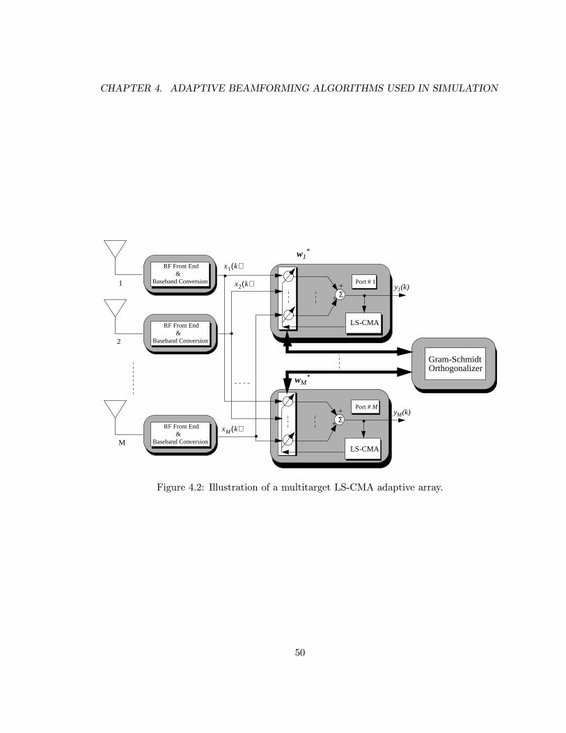
CHAPTER 4. ADAPTIVE BEAMFORMING ALGORITHMS USED IN SIMULATION
Σ+
+ .Port #M
yM(k)
RF Front End&
Baseband Conversion
RF Front End&
Baseband Conversion
RF Front End&
Baseband Conversion
Σ+
+ .Port # 1
y1(k)1
M
x1 k( )
2
x2 k( )
xM k( )
w1*
wM*
.
.
.
Gram-SchmidtOrthogonalizer
LS-CMA
LS-CMA
Figure 4.2: Illustration of a multitarget LS-CMA adaptive array.
50
CHAPTER 4. ADAPTIVE BEAMFORMING ALGORITHMS USED IN SIMULATION
are calculated using equation (4.1). The orthonormal basis W for the range of W is also
computed by using Gram-Schmidt orthogonalization procedure, where
W = [w1,w2, . . . ,wM ] (4.2)
W = [w1, w2, . . . , wM ] . (4.3)
The absolute values of the correlation coefficients are then compared to the threshold ρtr.
If for one i, i = 2, 3, . . . ,M , there exists one j < i such that |ρij | > ρtr, wi will be replaced
by a scaled version of wi, ‖wi‖ wi. After the GSO, the weight vectors are again adapted
by using the LS-CMA and the above procedure is repeated until the algorithm converges.
The orthonormal basis W for the range of W can be obtained by using the Gram-
Schmidt orthogonalization procedure which is described as follows [55]:
1. Given W = [w1,w2, . . . ,wM ], i = 1
2. w1 = w1‖w1‖
3. i = i+ 1
ρij =wHi wj
‖wi‖ ‖wj‖, j = 1, . . . , i− 1 (4.4)
wi = wi −i−1∑j=1
ρijwj (4.5)
wi =wi
‖wi‖(4.6)
4. Repeat step 3 until i = M .
A MATLABTM routine, Program [P3], is used to implement the GSO procedure.
The choice of the threshold ρtr will affect the convergence speed of the MT-LSCMA. If
ρtr is too small, two weight vectors that will not converge to one having the same beampat-
tern may be mis-identified as those intending to, and one of them will be replaced by the
51

CHAPTER 4. ADAPTIVE BEAMFORMING ALGORITHMS USED IN SIMULATION
scaled column vector of W. This new weight vector must be adapted for another several
iterations to converge but may be replaced again by the GSO output vector if the threshold
is too low. Apparently, this will decrease the convergence speed of the algorithm or even
cause the algorithm to diverge. On the other hand, if ρtr is too large, two weight vectors
that intend to converge to one having the same beampattern may not be identified, and the
algorithm may fail to form different beams directed to different users. In the simulations
performed in this research, 0.7 is found to be a good value of ρtr through experiments.
There is no need to perform the GSO once per iteration since the weight vectors adapted
after only one iteration are not well converged, and the correlation coefficients then calcu-
lated do not well represent the potential convergence of the weight vectors. Instead, the
GSO can be performed once per several iterations (i. e., five iterations) to reduce the com-
putational complexity of the algorithm.
4.3.2 Phase Ambiguity
Since MT-LSCMA uses the LS-CMA to adapt the weight vector for each port, and
as shown in section 3.3.2, the CMA-type algorithms suffer the phase ambiguity problem,
the phase of the signal at each output port is indeterminate. This problem can be solved
by three methods. The first method is to use the differential phase-shift keying (DPSK)
modulation in the CDMA system. Since in the DPSK modulation, it is the phase difference
between the current symbol and the previous symbol that determines the output data, a
phase rotation does not affect the demodulated data. The second method is to send a pilot
signal from the mobile to the base station and use the received pilot signal to obtain the
phase rotation information. This information can then be used to compensate the phase
ambiguity in the output port. The last method is to use the phase-constraint technique [29].
That is, add a phase constraint to each weight vector such that the first element of each
weight vector is a real number. For a weight vector wi after convergence, the new weight
52

CHAPTER 4. ADAPTIVE BEAMFORMING ALGORITHMS USED IN SIMULATION
vector wi generated by using phase-constraint is given by
wi = wi exp{−j arg(w1i)}, (4.7)
where arg[·] denotes the phase function and w1i is the first element of the weight vector wi.
4.3.3 Sorting Procedure
In MT-LSCMA, after the algorithm converges, a sorting procedure must be performed
to relate the port outputs to each user’s signal. In a CDMA system, the pseudo-noise
(PN) sequence assigned to each user can be utilized in the sorting procedure. For a CDMA
system with p users, the complex envelope of the signal transmitted by the ith user can be
expressed as
si(t) =√
2Pibi(t)ci(t) exp{−jφi}, i = 1, 2, . . . , p, (4.8)
where Pi, bi(t), ci(t), and φi are the power, the data signal, the spreading signal (PN
sequence), and the random phase of the ith user signal, respectively. The data signal bi(t)
is given by
bi(t) =∞∑
n=−∞binPTb(t− nTb), (4.9)
where bin ∈ {−1,+1} is the nth data bit of ith user, and PTb is a unit rectangular pulse of
duration Tb. Tb is the bit period of the CDMA signal. The spreading signal ci(t) is given
by
ci(t) =∞∑
m=−∞cimPTc(t−mTc), (4.10)
where cim ∈ {−1,+1} is the mth chip of ith user, and PTc is a unit rectangular pulse of
duration Tc. Tc is the chip period of the CDMA signal. The ratio of the bit period to the
chip period is called the processing gain and is defined as
Nc4=TbTc. (4.11)
Usually, systems are designed to have high processing gain where
Nc � 1 (4.12)
53

CHAPTER 4. ADAPTIVE BEAMFORMING ALGORITHMS USED IN SIMULATION
or equivalently,
Tb � Tc. (4.13)
The PN codes are also designed to have low cross-correlation and narrow autocorrelation
function.
Now, let’s assume the number of users in the system is less than or equal to the number
of the output ports in the beamformer. Also, the multipath and the interference of one
desired user are rejected due to the spatial filtering. Let’s further assume we have perfect
power control in the system, the output of port i in the beamformer is therefore a delayed,
scaled, and phase-rotated version of sj(t) which is corrupted by noise and is given by
yi(t) = αi√
2Pjbj(t− τj)cj(t− τj) exp{−j(φj + γi)}+ ni(t), (4.14)
where αi is the scaled factor for user i such that α2iPi = α2
jPj for i 6= j, τj is the time delay
of the jth user, γi is the phase shift in port i due to the phase rotation in LS-CMA, and
ni(t) is the AWGN noise in port i. In equation (4.14), i may or may not be equal to j, and
the sorting procedure is used to relate the user index i to the port index j. Let’s assume
the time delay τj is estimated perfectly, and the phase φj + γi is also estimated correctly
by using the method discussed in section 4.3.2, the sorting procedure can be performed
as shown in Figure 4.3. In Figure 4.3, y(t) is a vector containing the port outputs of the
beamformer and is given by
y(t) = [y1(t), y2(t), . . . , yM (t)]T (4.15)
The M output signals in y(t) are first multiplied by the delayed versions of p users’ PN
codes. So for each arm in Figure 4.3, there are M multiplying outputs corresponding to one
user’s PN code. These outputs are then integrated over one bit period, and the integration
outputs are sampled and their absolute values are compared with each other. Actually, the
output of the jth integrater in arm i is the correlation value between yj(t) and the delayed
PN code of user i, ci(t− τi). Since the PN codes are designed to have low cross correlation,
54

CHAPTER 4. ADAPTIVE BEAMFORMING ALGORITHMS USED IN SIMULATION
Comparison
Comparison
Comparison
jp
j1
j2
c1(t-τ1)
c2(t-τ2)
cp(t-τp)
y(t)∫0
Tb
∫0
Tb
∫0
Tb
Figure 4.3: Illustration of sorting procedure in MT-LSCMA for a CDMA system.
55

CHAPTER 4. ADAPTIVE BEAMFORMING ALGORITHMS USED IN SIMULATION
only the output port containing the ith user’s signal will have a peak at the integration
output. In arm i, the output port with the highest absolute value of the integrate output
will be identified as one containing the ith user’s signal, and the index of this output port,
ji, will be stored as the output of the sorting procedure.
If the number of users in the system is greater than the number of output ports, i. e.,
the number of antenna elements for this specific algorithm, one output port may contain
several user’s signals. Using the sorting procedure shown in Figure 4.3, we may relate one
output port with several users. In other words, there exist i1 and i2, where i1 6= i2, such
that ji1 = ji2 . In this case, the output of port ji1 (or ji2) will be fed into both user i1 and
user i2’s receivers to extract their signals.
If the above procedure is performed by using a digital system, the analog signals will
be replaced by their discrete time samples and the integration will be substituted by the
accumulated sum.
The MT-LSCMA can be summarized as follows:
1. Initialize the M weight vectors w1, . . . ,wM as the column vectors of a M×M identity
matrix.
2. Adapt each weight vector independently using the LS-CMA described in section 3.3.2.
3. After several iterations in LS-CMA, perform the GSO on the resulting weight vectors
as described in section 4.3.1.
4. Repeat step 2 and 3 until the algorithm converges.
5. Add the phase constraint or perform phase rotation compensation on the resulting
weight vectors as described in section 4.3.2.
56

CHAPTER 4. ADAPTIVE BEAMFORMING ALGORITHMS USED IN SIMULATION
6. Perform the sorting procedure described in section 4.3.3 to relate the output ports to
each user’s signal.
4.4 Multitarget Decision-Directed Algorithm
By replacing LS-CMA in the MT-LSCMA with decision-directed (DD) algorithm de-
scribed in section 3.3.4, we obtain the MT-DD algorithm. The DD algorithm can be per-
formed with either the steepest-descent (SD) method or the least-squares (LS) method.
If the DD algorithm in the MT-DD is performed with steepest-decent method, we will
call this multitarget-type algorithm the multitarget steepest-descent decision-directed (MT-
SDDD) algorithm, and if the DD algorithm in the MT-DD is performed with least-squares
method, we will call it the multitarget least-squares decision-directed (MT-LSDD) algorithm.
The SD-DD algorithm is described by equation (3.65), (3.66), and ( 3.67). The LS-DD
algorithm can be derived in the same manner as that of the LS-CMA algorithm and can be
described as
y(l) =[wH(l)X(l)
]T= [y(1 + lK), y(2 + lK), . . . , y((l + 1)K)]T (4.16)
r(l) = [sgn{Re(y(1 + lK))}, . . . , sgn{Re(y((l + 1)K))}]T (4.17)
w(l + 1) =[X(l)XH(l)
]−1X(l)r∗(l) (4.18)
where l is the iteration number, X(l) is defined in equation (3.55), and K is the number of
samples in one data block.
Unlike the MT-LSCMA which constrains the signal constellations on the unit circle, the
MT-DD algorithm constrains the signal constellations at either +1 or −1. Since the signal
of each user has a random phase, this constraint will also cause a phase ambiguity. The
methods introduced in section 4.3.2 can be used to compensate this effect.
57

CHAPTER 4. ADAPTIVE BEAMFORMING ALGORITHMS USED IN SIMULATION
The MT-SDDD algorithm can be described as follows:
1. Initialize the M weight vectors w1, . . . ,wM as the column vectors of a M×M identity
matrix.
2. Adapt each weight vector independently using the SD-DD described in section 3.3.4.
3. After a number of iterations in SD-DD, perform the GSO on the resulting weight
vectors as described in section 4.3.1.
4. Repeat step 2 and 3 until the algorithm converges.
5. Add the phase constraint or perform phase rotation compensation on the resulting
weight vectors as described in section 4.3.2.
6. Perform the sorting procedure described in section 4.3.3 to relate the output ports to
each user’s signal.
In step 2, the number of iterations needed before the GSO depends on the step size µ in
the SD-DD algorithm. In our simulation, µ is set to 0.001 and the number of iterations
before the GSO is set to 1000. In MT-LSDD, the number of iterations needed will be
around 5 as that in MT-LSCMA, but for both the MT-LSDD and MT-LSCMA, the matrix
inversion has to be calculated. So there is a trade-off between the convergence speed and
the computational complexity.
4.5 Least-Squares Despread Respread Multitarget Array
The multitarget adaptive algorithms discussed to date do not utilize any information of
the spreading signal of each user in the CDMA system. However, in a CDMA system, it is
these spreading signals that distinguish different users occupying the same frequency band.
Therefore it will be very useful if the information of these spreading signals can be utilized
in the multitarget adaptive algorithm. In this section and section 4.6 we will introduce two
novel algorithms developed in this research that utilize the information of the spreading
58
CHAPTER 4. ADAPTIVE BEAMFORMING ALGORITHMS USED IN SIMULATION
signals. The algorithm discussed in this section is called least-squares despread respread
multitarget array (LS-DRMTA).
4.5.1 Derivation of LS-DRMTA
In the base station of a CDMA system, the spreading signals of all the users are known
beforehand. In the conventional receiver, to detect the ith user’s data bits, the received
signal is correlated with the time-delayed spreading signal of the ith user, ci(t− τi), and the
correlation output is sent to the detector, which makes a decision based on the correlation
output. There exist many techniques to detect the time delay, τi, for the ith user, and we
are not going to cover this topic in this research. So from now on, we assume that the time
delay for each user is detected perfectly unless specified otherwise. The effect of the error
of the time delay estimation on the performance of the algorithm is discussed in section 5.4.
If the nth data bit of the ith user is detected correctly by the detector, i. e., bin = bin,
where bin is the detector output, the waveform of the ith user’s transmitted signal dur-
ing time period [(n − 1)Tb, nTb) can be obtained by respreading the detected data bit bin
with the PN sequence of the ith user, ci(t). This respread signal can then be used in the
beamformer to adapt the weight vector for user i. The adaptive algorithm that uses this
despread-and-respread technique is referred to as least-squares despread respread multitarget
array (LS-DRMTA) in this research. Figure 4.4 shows the structure of a beamformer using
the LS-DRMTA and Figure 4.5 shows the block diagram of the LS-DRMTA for user i. Note
that in Figure 4.4, the number of beamformer output ports is now equal to the number of
users in the system.
In Figure 4.5, ri(t) is a time-delayed version of the respread signal for user i and is given
by
ri(t) = binci(t− τi), (n− 1)Tb ≤ t < nTb. (4.19)
In a conventional CDMA system, the PN sequence is repeated every bit period, therefore
59
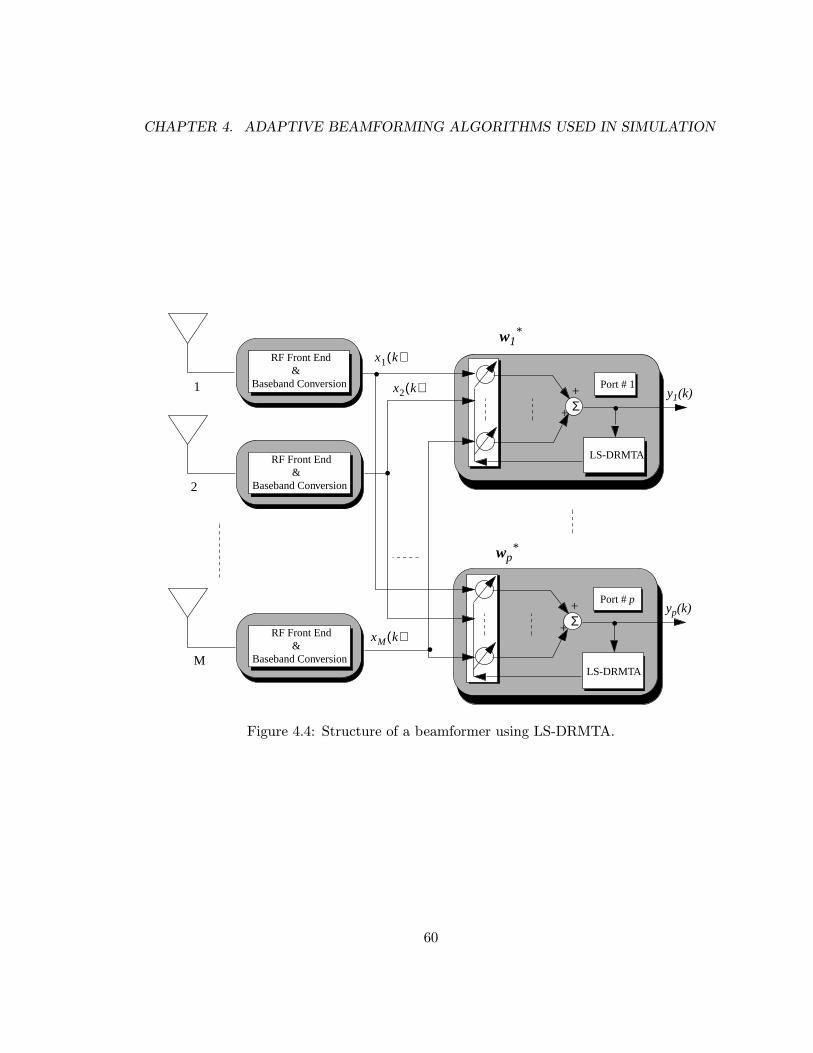
CHAPTER 4. ADAPTIVE BEAMFORMING ALGORITHMS USED IN SIMULATION
Σ+
+ .Port #p
yp(k)
RF Front End&
Baseband Conversion
RF Front End&
Baseband Conversion
RF Front End&
Baseband Conversion
Σ+
+ .Port # 1
y1(k)1
M
x1 k( )
2
x2 k( )
xM k( )
w1*
wp*
.
.
.
LS-DRMTA
LS-DRMTA
Figure 4.4: Structure of a beamformer using LS-DRMTA.
60

CHAPTER 4. ADAPTIVE BEAMFORMING ALGORITHMS USED IN SIMULATION
ci(t-τi)
∫0
Tb
ci(t)
delay τi
yi(t)
wi ri(t)
bin^
Extensionof Gauss’ Method
Figure 4.5: LS-DRMTA block diagram for user i.
both ci(t) and ri(t) have a time period Tb. Let yi(k) and ri(k) denote the kth sample of
yi(t) and ri(t), respectively, in a digital system, the LS-DRMTA tries to adapt the weight
vector wi to minimize the cost function
F (wi) =K∑k=1
|yi(k)− ri(k)|2
=K∑k=1
∣∣∣wHi x(k)− ri(k)
∣∣∣2 , (4.20)
where K is the data block size and is set to be equal to the number of samples in one bit
period in LS-DRMTA. So if the signal is sampled with a sampling rate Rs = NsRc, where
Rc is the chip rate of the CDMA signal, and Ns is an integer greater than two, the block size
K will be equal to NcNs, where Nc is the processing gain. Using the extension of Gauss’
method described in section 3.3.2 and comparing equation (4.20) with (3.36), we have
gk(wi) = |yi(k)− ri(k)|
=∣∣∣wH
i x(k)− ri(k)∣∣∣ . (4.21)
61

CHAPTER 4. ADAPTIVE BEAMFORMING ALGORITHMS USED IN SIMULATION
Substituting equation (4.21) into (3.37), we obtain
g(wi) =
|yi(1) − ri(1)|
|yi(2) − ri(2)|...
|yi(k)− ri(k)| .
(4.22)
The gradient vector of gk(wi) is given by
∇ (gk(wi)) = 2∂gk(wi)
∂w∗i
= x(k)[yi(k) − ri(k)]∗
|yi(k)− ri(k)| . (4.23)
Let
vi(k) = yi(k)− ri(k) (4.24)
equation (4.23) can be expressed as
∇ (gk(wi)) = x(k)v∗i (k)
|vi(k)| . (4.25)
Substituting equation (4.25) into (3.39), D(wi) can be expressed as
D(wi) = [∇ (g1(wi)) ,∇ (g2(wi)) , . . . ,∇ (gK(wi))]
=
[x(1)
v∗i (1)
|vi(1)| ,x(2)v∗i (2)
|vi(2)| , . . . ,x(K)v∗i (K)
|vi(K)|
]= XViCM , (4.26)
where
X = [x(1),x(2), . . . ,x(K)], (4.27)
and
ViCM =
v∗i (1)|vi(1)| 0 · · · 0
0v∗i (2)|vi(2)|
......
. . . 0
0 · · · 0v∗i (K)|vi(K)|
. (4.28)
62
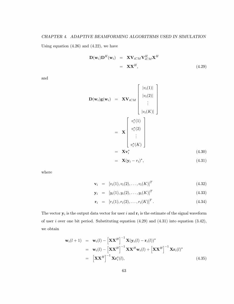
CHAPTER 4. ADAPTIVE BEAMFORMING ALGORITHMS USED IN SIMULATION
Using equation (4.26) and (4.22), we have
D(wi)DH(wi) = XViCMVH
iCMXH
= XXH , (4.29)
and
D(wi)g(wi) = XViCM
|vi(1)|
|vi(2)|...
|vi(K)|
= X
v∗i (1)
v∗i (2)...
v∗i (K)
= Xv∗i (4.30)
= X(yi − ri)∗, (4.31)
where
vi = [vi(1), vi(2), . . . , vi(K)]T (4.32)
yi = [yi(1), yi(2), . . . , yi(K)]T (4.33)
ri = [ri(1), ri(2), . . . , ri(K)]T . (4.34)
The vector yi is the output data vector for user i and ri is the estimate of the signal waveform
of user i over one bit period. Substituting equation (4.29) and (4.31) into equation (3.42),
we obtain
wi(l + 1) = wi(l)−[XXH
]−1X(yi(l)− ri(l))
∗
= wi(l)−[XXH
]−1XXHwi(l) +
[XXH
]−1Xri(l)
∗
=[XXH
]−1Xr∗i (l), (4.35)
63

CHAPTER 4. ADAPTIVE BEAMFORMING ALGORITHMS USED IN SIMULATION
where yi(l) and ri(l) are the output data vector and estimate of signal waveform of user i
over one bit period corresponding to the weight vector wi in the lth iteration, respectively.
Similar to the dynamic LS-CMA, LS-DRMTA can adapt the weight vectors using different
input data blocks in each iteration. Let
X(l) = [x(1 + lK),x(2 + lK), . . . ,x((l + 1)K)] , l = 0, 1, . . . , L, (4.36)
where L is the number of iterations required for the algorithm to converge, and K is the
number of data samples per bit (NcNs) if the data samples over one bit period are all used
for the adaptation. In Figure 4.4, the LS-DRMTA for the ith user can be described by the
following equations
yi(l) =[wHi (l)X(l)
]T= [yi(1 + lK), yi(2 + lK), . . . , yi((l + 1)K)]T (4.37)
bil = sgn
Re
(1+l)K∑k=1+lK
yi(k)ci(k − kτi)
(4.38)
ri(l) = bil [ci(1 + lK − kτi), ci(2 + lK − kτi), . . . , ci((1 + l)K − kτi)]T (4.39)
wi(l + 1) =[X(l)XH(l)
]−1X(l)r∗i (l), (4.40)
where ci(k) is the kth sample of the spreading signal of user i, kτi is the number of samples
corresponding to τi, the delay of user i, and bil is the estimate of lth bit for user i. The ac-
cumulated sum in equation (4.38) is equivalent to integration in the continuous time domain.
We can summarize the LS-DRMTA as follows
1. Initialize the p weight vectors w1, . . . ,wp as p identical M × 1 column vectors with
the first element equal to 1 and the other elements equal to 0.
2. Calculate the array output vector using equation (4.37).
3. Despread the ith user’s signal and estimate the nth data bit using equation (4.38).
64
CHAPTER 4. ADAPTIVE BEAMFORMING ALGORITHMS USED IN SIMULATION
4. Respread the estimate data bit with the PN code of user i to get a estimate of the
signal waveform of user i over time period [(n− 1)Tb, nTb) using equation (4.39).
5. Adapt the weight vector wi of user i using equation (4.40).
6. Repeat step 2 to 5 until the algorithm converges.
In equation (4.39), when l = 0, there may be some time indices less than zero, but since
the PN sequence has a time period of Tb, or equivalently, a period of K in the discrete time
domain, the index k, where k < 0, can be replaced by the index k +K.
In LS-DRMTA, if the data bit is not estimated correctly at the beginning of the algo-
rithm, from equation (4.39) and (4.40) we see that the resulting weight vector may have a
phase shift of π, but this does not affect the resulting beampattern. The beampattern will
still have a higher gain in the DOA of the desired signal and the interference from other
directions will be rejected. Therefore if the DPSK modulation is used in the system, the
data bit estimation error at the beginning of the algorithm does not affect the demodulated
data bit.
4.5.2 Advantages of LS-DRMTA
Since the LS-DRMTA utilizes the information of each user’s spreading signal to adapt
the weight vectors, it has several advantages over the two algorithms, MT-LSCMA, and
MT-SDDD, discussed in previous sections.
The first advantage of the LS-DRMTA is that there is no need to perform the GSO
procedure. This can be seen by comparing Figure 4.4 with Figure 4.2. In MT-LSCMA and
MT-SDDD, the weight vectors are adapted by using the same property of all the user’s
signal, and the GSO procedure is used to prevent different weight vectors from converging
to one having the same beampattern. In LS-DRMTA, however, different users’ weight vec-
tor are adapted to minimize a different cost function, which is a sum of the squared error
65

CHAPTER 4. ADAPTIVE BEAMFORMING ALGORITHMS USED IN SIMULATION
between the port output and the respread signal of the desired user over one bit period.
Since each different user has a different spreading signal, the weight vector of each different
user is updated with a different tendency and thus will not converge to one having the same
beampattern.
The second advantage of the LS-DRMTA is that there is no need to perform the sorting
procedure. In MT-LSCMA and MT-SDDD, the sorting procedure is used to relate each
output port to each user. In LS-DRMTA, since different weight vectors are adapted with
different PN sequences, the weight vector adapted by using the ith user’s spreading signal
will be corresponding to the ith user. Therefore there is no need to perform the sorting
procedure.
The third advantage of the LS-DRMTA is that the number of output ports of the beam-
former is not limited by the number of antenna elements of the array. In MT-LSCMA and
MT-SDDD, due to the GSO procedure, the number of output ports should be less than or
equal to the number of antenna elements. If the number of users in the system is greater
than the number of antenna elements, several users have to share one output port, and the
interference cannot be reduced to a very low level. In LS-DRMTA, since there is no GSO
needed, the number of output ports can be equal to the number of users even if the number
of users is greater than the number of antenna elements. Since each user has its own output
port, the interference can be reduced to a lower level. Furthermore, if the system is ex-
panded, more output ports can be added to the beamformer easily by adding more weight
vectors adapted with the PN sequences of the new users. As shown in Figure 4.4, the new
output ports use the same array input data vector, so no new RF front end and baseband
conversion are needed, which will reduce the cost of the adaptive antenna system.
The fourth advantage of the LS-DRMTA is that the computational complexity of the
LS-DRMTA is lower than that of the MT-LSCMA and MT-SDDD. In MT-LSCMA and
66

CHAPTER 4. ADAPTIVE BEAMFORMING ALGORITHMS USED IN SIMULATION
MT-SDDD, both the GSO procedure and the sorting procedure have to be performed to
extract different user’s signal. From the previous discussion we see that these two proce-
dures are very computationally intensive. LS-DRMTA, on the other hand, eliminates these
two procedures and therefore requires lower computational complexity.
The last advantage of the LS-DRMTA is that it can work under the condition where
the SINR is low and both the MT-LSCMA and MT-SDDD cannot work. In LS-DRMTA,
the PN sequence is used in the adaptation of the weight vector, and these PN sequence
may spread the interference over a large frequency band and despread the desired signal.
Also the noise is averaged over one bit period in LS-DRMTA and their effect on the desired
signal is reduced. So the LS-DRMTA can work in a low SINR situation.
4.6 Least-Squares Despread Respread Multitarget Constant Modulus Al-
gorithm
In LS-DRMTA, we utilize the spreading signal of each user in a CDMA system to adapt
the weight vectors of the beamformer. In MT-LSCMA, on the other hand, we utilize the
constant modulus property of the transmitted signal to update the weight vectors. One
intuitive thought is to combine the spreading signal and the constant modulus property of
the transmitted signal to adapt the weight vector. The algorithm using this kind of combi-
nation in the adaptation of the weight vector is referred to as least-squares despread respread
multitarget constant modulus algorithm (LS-DRMTCMA) in this research. Figure 4.6 shows
the structure of a beamformer using the LS-DRMTCMA and Figure 4.7 shows the block
diagram of the LS-DRMTCMA for user i.
4.6.1 Derivation of LS-DRMTCMA
The derivation of the LS-DRMTCMA is very similar to that of the LS-DRMTA. In LS-
DRMTA, the cost function that the algorithm wants to minimize is given in equation (4.41)
67

CHAPTER 4. ADAPTIVE BEAMFORMING ALGORITHMS USED IN SIMULATION
Σ+
+ .Port #p
yp(k)
RF Front End&
Baseband Conversion
RF Front End&
Baseband Conversion
RF Front End&
Baseband Conversion
Σ+
+ .Port # 1
y1(k)1
M
x1 k( )
2
x2 k( )
xM k( )
w1*
wp*
.
.
.
LS-DRMTCMA
LS-DRMTCMA
Figure 4.6: Structure of a beamformer using LS-DRMTCMA.
68

CHAPTER 4. ADAPTIVE BEAMFORMING ALGORITHMS USED IN SIMULATION
ci(t-τi)
∫0
Tb
ci(t)
delay τi
yi(t)
wi
ri(t)
bin^
Extensionof Gauss’ Method
yi t( )yi t( )--------------
Σ+ +
aPNaCM
riCM(t) riPN(t)
Figure 4.7: LS-DRMTCMA block diagram for user i.
69
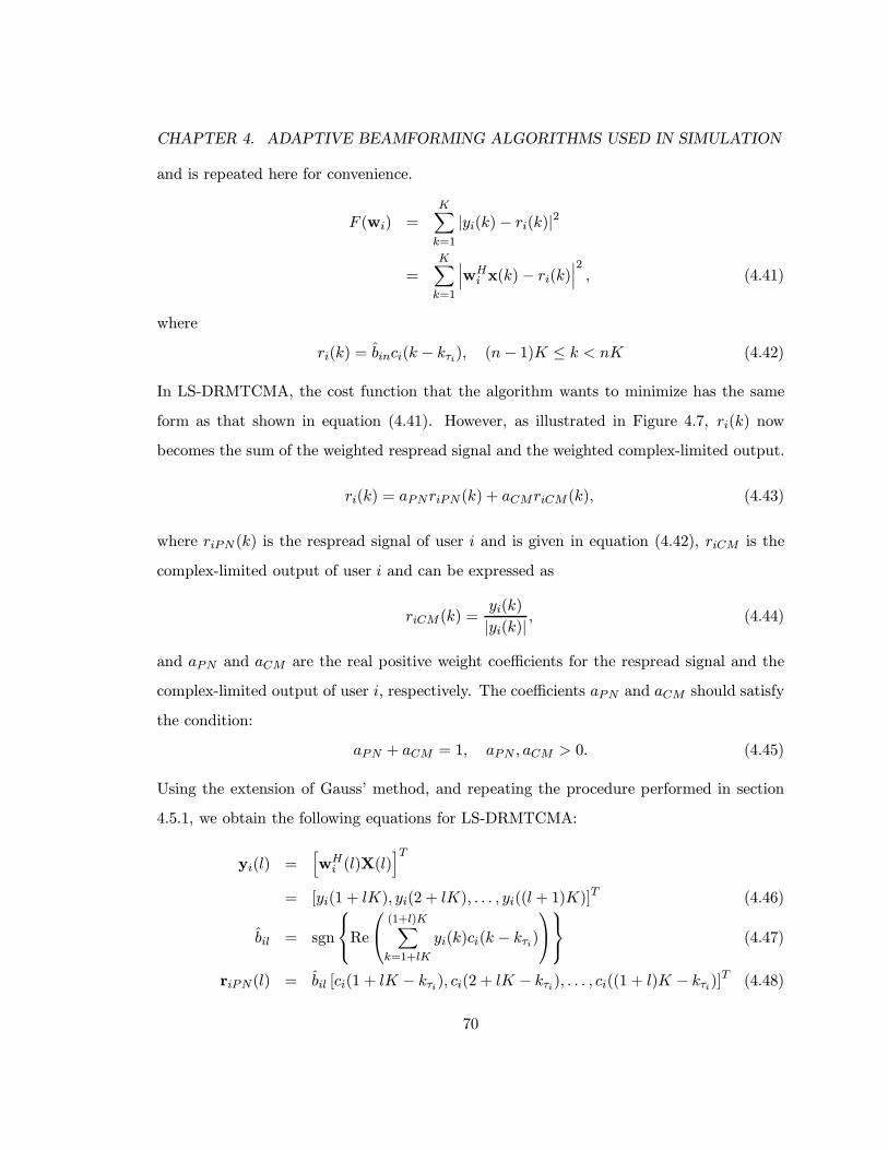
CHAPTER 4. ADAPTIVE BEAMFORMING ALGORITHMS USED IN SIMULATION
and is repeated here for convenience.
F (wi) =K∑k=1
|yi(k)− ri(k)|2
=K∑k=1
∣∣∣wHi x(k)− ri(k)
∣∣∣2 , (4.41)
where
ri(k) = binci(k − kτi), (n − 1)K ≤ k < nK (4.42)
In LS-DRMTCMA, the cost function that the algorithm wants to minimize has the same
form as that shown in equation (4.41). However, as illustrated in Figure 4.7, ri(k) now
becomes the sum of the weighted respread signal and the weighted complex-limited output.
ri(k) = aPNriPN (k) + aCMriCM (k), (4.43)
where riPN (k) is the respread signal of user i and is given in equation (4.42), riCM is the
complex-limited output of user i and can be expressed as
riCM (k) =yi(k)
|yi(k)| , (4.44)
and aPN and aCM are the real positive weight coefficients for the respread signal and the
complex-limited output of user i, respectively. The coefficients aPN and aCM should satisfy
the condition:
aPN + aCM = 1, aPN , aCM > 0. (4.45)
Using the extension of Gauss’ method, and repeating the procedure performed in section
4.5.1, we obtain the following equations for LS-DRMTCMA:
yi(l) =[wHi (l)X(l)
]T= [yi(1 + lK), yi(2 + lK), . . . , yi((l + 1)K)]T (4.46)
bil = sgn
Re
(1+l)K∑k=1+lK
yi(k)ci(k − kτi)
(4.47)
riPN(l) = bil [ci(1 + lK − kτi), ci(2 + lK − kτi), . . . , ci((1 + l)K − kτi)]T (4.48)
70

CHAPTER 4. ADAPTIVE BEAMFORMING ALGORITHMS USED IN SIMULATION
riCM (l) =
[y(1 + lK)
|y(1 + lK)| ,y(2 + lK)
|y(2 + lK)| , . . . ,y((1 + l)K)
|y((1 + l)K)|
]T(4.49)
ri(l) = aPNriPN(l) + aCMriCM (l) (4.50)
wi(l + 1) =[X(l)XH(l)
]−1X(l)r∗i (l). (4.51)
From the above equations we see that if aCM is set to zero, the LS-DRMTCMA becomes
the LS-DRMTA, therefore the LS-DRMTA can be viewed as a special case of the LS-
DRMTCMA. Also we see that if aPN is set to zero and the GSO procedure is performed
during the adaptation, the algorithm becomes MT-LSCMA. The choice of aPN and aCM
can affect the resulting beampattern and thus the performance of the system. We will
demonstrate this point by simulation in Chapter 5.
We can summarize the LS-DRMTCMA as follows
1. Initialize the p weight vectors w1, . . . ,wp as p identical M × 1 column vectors with
the first element equal to 1 and the other elements equal to 0.
2. Calculate the array output vector using equation (4.46).
3. Despread the ith user’s signal and estimate the nth data bit using equation (4.47).
4. Respread the estimate data bit with the PN code of user i to get a estimate of the
signal waveform of user i over time period [(n− 1)Tb, nTb) using equation (4.48).
5. Calculate the complex-limited output vector of user i using equation (4.49).
6. Calculate the reference signal vector for user i by summing up the weighted respread
signal vector and the weighted complex-limited output vector using equation (4.50).
7. Adapt the weight vector wi of user i using equation (4.51).
8. Repeat step 2 to 7 until the algorithm converges.
71

CHAPTER 4. ADAPTIVE BEAMFORMING ALGORITHMS USED IN SIMULATION
4.6.2 Advantages of LS-DRMTCMA
Since the LS-DRMTCMA utilize both the PN sequence and the constant modulus prop-
erty of the transmitted signal, it possesses all the advantages of LS-DRMTA and has other
advantages that the LS-DRMTA does not possess. The most important advantage is that
it can achieve a much lower BER than the LS-DRMTA. We will discuss this point in Chap-
ter 5. However, since LS-DRMTCMA utilizes the complex-limited output vector of each
user in the adaptation of the weight vectors, this advantage is achieved at the expense of
additional complexity.
4.7 Summary
In this chapter we present four multitarget-type blind adaptive beamformer algorithms,
MT-LSCMA, MT-DD, LS-DRMTA, and LS-DRMTCMA. The LS-DRMTA and the LS-
DRMTCMA are two novel algorithms developed in this research. The derivation and the
advantages of these two novel algorithms are described. In Chapter 5, we will present the
simulation results and compare these four algorithms.
72
Chapter 5
Simulation Results and Discussion
5.1 Introduction
In Chapter 4 we present four multitarget-type adaptive beamformer algorithms for the
base station in a CDMA system. In this chapter, we will compare these four algorithms
under different conditions. The following four cases will be considered in the simulation:
1. AWGN channel
2. System with timing offset
3. System with frequency offset
4. Multipath channel.
Our comparison of the algorithms will focus on the BER performance of different algorithms.
The convergence characteristics of the different algorithms will also be presented.
5.2 Description of System Parameters
The system we consider in the simulation is a direct sequence CDMA (DS-CDMA)
system with a processing gain, N , equal to 15. There are several reasons for choosing such
a small processing gain. The first reason is that we want to reduce the simulation time
and at the same time compare the performance of different adaptive algorithms in a CDMA
system. The second one is that we want to focus on the enhancement of the system capacity
obtained by utilizing the adaptive array, not on the enhancement obtained by using a long
PN sequence for each user. The last one is that N = 15 is the parameter specified by the
73

CHAPTER 5. SIMULATION RESULTS AND DISCUSSION
GLOMO program. The modulation scheme used in the system is the binary phase-shift
keying (BPSK), the carrier frequency fc is equal to 2.05 GHz, and the data bit rate Rb
is equal to 128 kbps. An 8-element uniform linear array with half wave-length spacing
between the elements is used in the base station of the system to perform spatial filtering
in the reverse link (from the mobile to the base station). The sampling rate is four times
the chip rate, in other words, there are four data samples per chip. So for the LS-DRMTA
and LS-DRMTCMA, the data block size is equal to 60, which is the number of samples per
bit.
5.3 Simulation Results in AWGN Channel
Let’s first consider one case where there are 8 users in the system transmitting CDMA
signals from different directions. The DOAs of the signals are equally spaced between −70◦
Table 5.1: Signal Parameters of 8 Users Transmitting Signals from Different Directions
User # Power (dBW) DOA (deg)
1 0 -70
2 0 -47
3 0 -24
4 0 -1
5 0 22
6 0 45
7 0 68
8 0 90
Eb/N0 = 20 dB
and 90◦. Figure 5.1 shows the distribution of these 8 users. We assume that there is no
multipath and the radio channel only introduces the additive white Gaussian noise (AWGN).
We also assume perfect power control in the base station, so all the signals impinging on
the array have the same power. The input signal to noise ratio per bit (Eb/N0) is set to 20
dB. Table 5.1 shows the signal parameters of all the user’s signal.
74
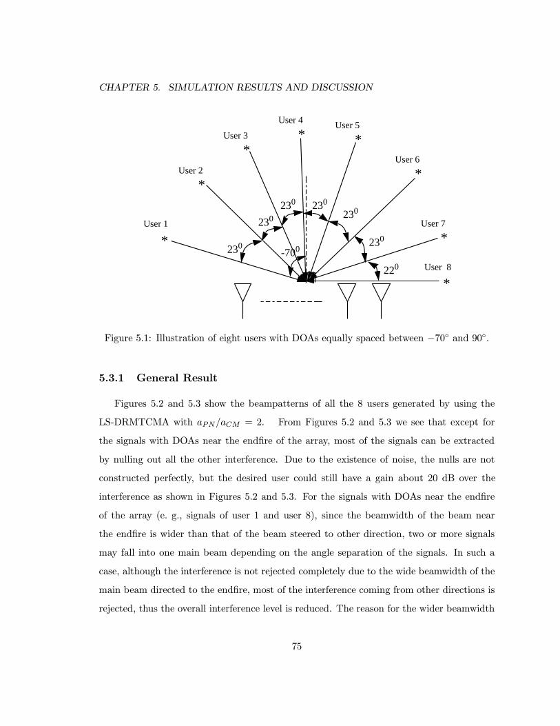
CHAPTER 5. SIMULATION RESULTS AND DISCUSSION
*
*
User 1
-700
User 2
*User 8
230
*User 3
230
230 230
230
220
230
*User 4
*User 5
*User 6
*User 7
Figure 5.1: Illustration of eight users with DOAs equally spaced between −70◦ and 90◦.
5.3.1 General Result
Figures 5.2 and 5.3 show the beampatterns of all the 8 users generated by using the
LS-DRMTCMA with aPN/aCM = 2. From Figures 5.2 and 5.3 we see that except for
the signals with DOAs near the endfire of the array, most of the signals can be extracted
by nulling out all the other interference. Due to the existence of noise, the nulls are not
constructed perfectly, but the desired user could still have a gain about 20 dB over the
interference as shown in Figures 5.2 and 5.3. For the signals with DOAs near the endfire
of the array (e. g., signals of user 1 and user 8), since the beamwidth of the beam near
the endfire is wider than that of the beam steered to other direction, two or more signals
may fall into one main beam depending on the angle separation of the signals. In such a
case, although the interference is not rejected completely due to the wide beamwidth of the
main beam directed to the endfire, most of the interference coming from other directions is
rejected, thus the overall interference level is reduced. The reason for the wider beamwidth
75
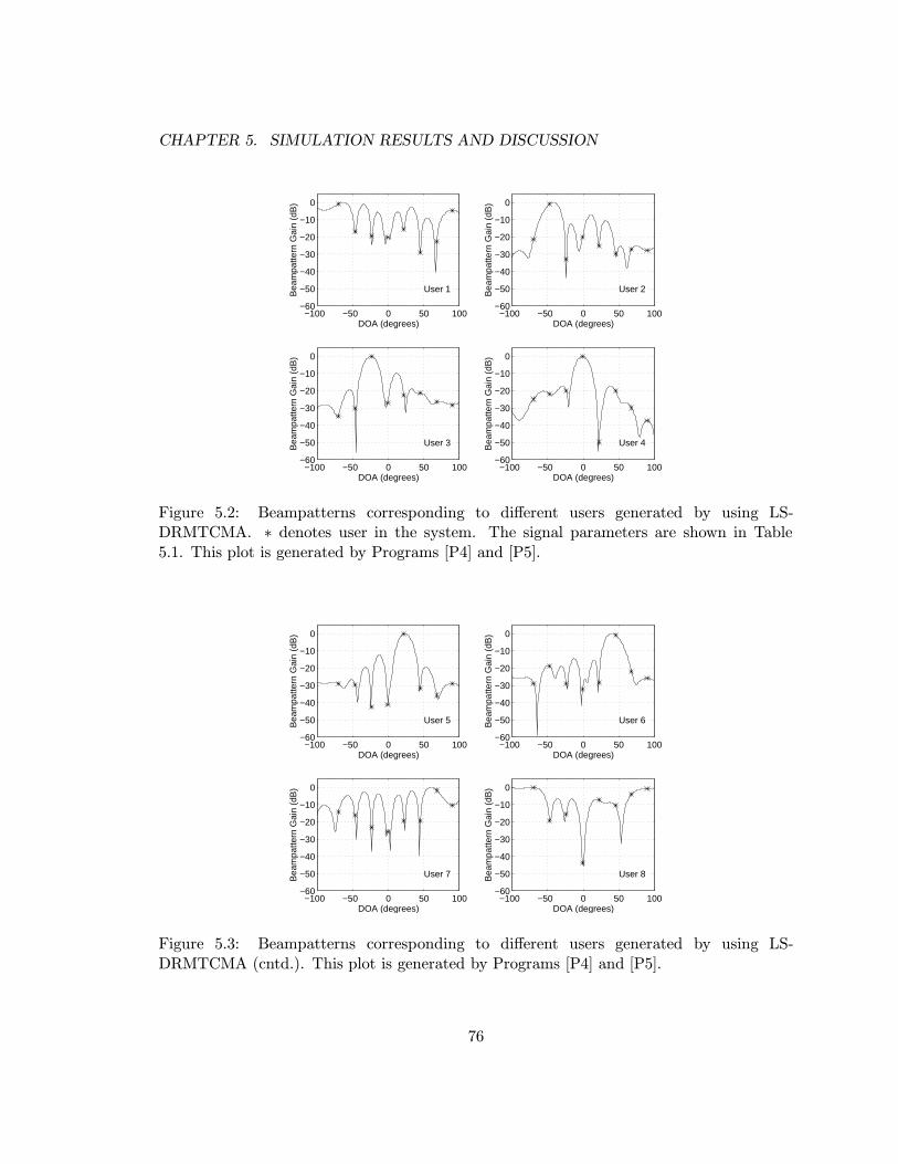
CHAPTER 5. SIMULATION RESULTS AND DISCUSSION
−100 −50 0 50 100−60
−50
−40
−30
−20
−10
0
DOA (degrees)
Bea
mpa
ttern
Gai
n (d
B)
User 1
−100 −50 0 50 100−60
−50
−40
−30
−20
−10
0
DOA (degrees)
Bea
mpa
ttern
Gai
n (d
B)
User 2
−100 −50 0 50 100−60
−50
−40
−30
−20
−10
0
DOA (degrees)
Bea
mpa
ttern
Gai
n (d
B)
User 3
−100 −50 0 50 100−60
−50
−40
−30
−20
−10
0
DOA (degrees)B
eam
patte
rn G
ain
(dB
)
User 4
Figure 5.2: Beampatterns corresponding to different users generated by using LS-DRMTCMA. ∗ denotes user in the system. The signal parameters are shown in Table5.1. This plot is generated by Programs [P4] and [P5].
−100 −50 0 50 100−60
−50
−40
−30
−20
−10
0
DOA (degrees)
Bea
mpa
ttern
Gai
n (d
B)
User 5
−100 −50 0 50 100−60
−50
−40
−30
−20
−10
0
DOA (degrees)
Bea
mpa
ttern
Gai
n (d
B)
User 6
−100 −50 0 50 100−60
−50
−40
−30
−20
−10
0
DOA (degrees)
Bea
mpa
ttern
Gai
n (d
B)
User 7
−100 −50 0 50 100−60
−50
−40
−30
−20
−10
0
DOA (degrees)
Bea
mpa
ttern
Gai
n (d
B)
User 8
Figure 5.3: Beampatterns corresponding to different users generated by using LS-DRMTCMA (cntd.). This plot is generated by Programs [P4] and [P5].
76

CHAPTER 5. SIMULATION RESULTS AND DISCUSSION
along the endfire of the array can be explained as follows. As shown in Chapter 2, the
sine of the DOA θ corresponds to the temporal frequency f of a FIR filter input, and
the beampattern of an adaptive array can be viewed as the counterpart of the magnitude
response of an FIR filter. So the passband-width ∆f of a FIR filter corresponds to the term
sin θ − sin(θ −∆θ) in the array, where ∆θ is the beamwidth of the main beam. If we want
to keep sin θ − sin(θ −∆θ) constant for all θ (like keeping the passband-width of the FIR
filter constant over all the frequency band), we have
sin θ − sin(θ −∆θ) = ∆f. (5.1)
The term in the left side of equation (5.1) can be expressed as
sin θ − sin(θ −∆θ) = ∆θ cos θ′
(5.2)
where θ′
is a value in [θ −∆θ, θ]. Substituting equation (5.2) into (5.1) we obtain
∆θ =∆f
cos θ′. (5.3)
From equation (5.3) we see that for a fixed ∆f , ∆θ will change with θ. For DOA near the
endfire of the array, θ, and therefore θ′, are close to π/2, so for a fixed passband-width,
∆θ will be large since cos θ′
is close to 0. On the other hand, for DOA near the broadside
of the array, θ′
is close to 0, and ∆θ will be small since cos θ′
is close to 1. Therefore the
beamformer can construct a narrow beam directed to the broadside of the array and a wide
beam directed to the endfire of the array.
The signal constellations of user 5 before and after the beamformer processing are shown
in Figure 5.4 and Figure 5.5, respectively. In Figure 5.5, we have compensated the random
phase effect by multiplying the beamformer output of user 5 by the complex conjugate of
exp{jφ5}, where φ5 is the random phase of user 5. Comparing Figure 5.4 and Figure 5.5, we
see that the interference from different DOAs is indeed rejected and the signal constellation
is reconstructed. Figures 5.6, 5.7, and 5.8 show the original signal waveform, the corrupted
77
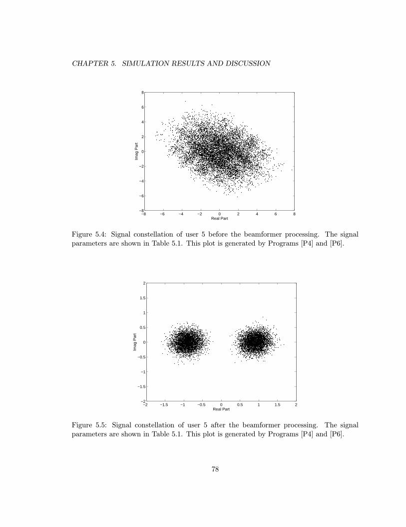
CHAPTER 5. SIMULATION RESULTS AND DISCUSSION
−8 −6 −4 −2 0 2 4 6 8−8
−6
−4
−2
0
2
4
6
8
Real Part
Imag
Par
t
Figure 5.4: Signal constellation of user 5 before the beamformer processing. The signalparameters are shown in Table 5.1. This plot is generated by Programs [P4] and [P6].
−2 −1.5 −1 −0.5 0 0.5 1 1.5 2−2
−1.5
−1
−0.5
0
0.5
1
1.5
2
Real Part
Imag
Par
t
Figure 5.5: Signal constellation of user 5 after the beamformer processing. The signalparameters are shown in Table 5.1. This plot is generated by Programs [P4] and [P6].
78
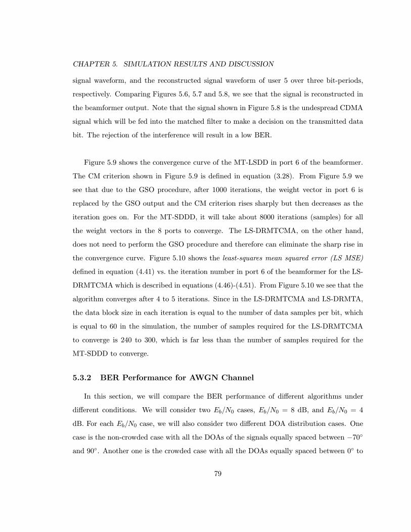
CHAPTER 5. SIMULATION RESULTS AND DISCUSSION
signal waveform, and the reconstructed signal waveform of user 5 over three bit-periods,
respectively. Comparing Figures 5.6, 5.7 and 5.8, we see that the signal is reconstructed in
the beamformer output. Note that the signal shown in Figure 5.8 is the undespread CDMA
signal which will be fed into the matched filter to make a decision on the transmitted data
bit. The rejection of the interference will result in a low BER.
Figure 5.9 shows the convergence curve of the MT-LSDD in port 6 of the beamformer.
The CM criterion shown in Figure 5.9 is defined in equation (3.28). From Figure 5.9 we
see that due to the GSO procedure, after 1000 iterations, the weight vector in port 6 is
replaced by the GSO output and the CM criterion rises sharply but then decreases as the
iteration goes on. For the MT-SDDD, it will take about 8000 iterations (samples) for all
the weight vectors in the 8 ports to converge. The LS-DRMTCMA, on the other hand,
does not need to perform the GSO procedure and therefore can eliminate the sharp rise in
the convergence curve. Figure 5.10 shows the least-squares mean squared error (LS MSE)
defined in equation (4.41) vs. the iteration number in port 6 of the beamformer for the LS-
DRMTCMA which is described in equations (4.46)-(4.51). From Figure 5.10 we see that the
algorithm converges after 4 to 5 iterations. Since in the LS-DRMTCMA and LS-DRMTA,
the data block size in each iteration is equal to the number of data samples per bit, which
is equal to 60 in the simulation, the number of samples required for the LS-DRMTCMA
to converge is 240 to 300, which is far less than the number of samples required for the
MT-SDDD to converge.
5.3.2 BER Performance for AWGN Channel
In this section, we will compare the BER performance of different algorithms under
different conditions. We will consider two Eb/N0 cases, Eb/N0 = 8 dB, and Eb/N0 = 4
dB. For each Eb/N0 case, we will also consider two different DOA distribution cases. One
case is the non-crowded case with all the DOAs of the signals equally spaced between −70◦
and 90◦. Another one is the crowded case with all the DOAs equally spaced between 0◦ to
79

CHAPTER 5. SIMULATION RESULTS AND DISCUSSION
20 40 60 80 100 120 140 160 180
−0.25
−0.2
−0.15
−0.1
−0.05
0
0.05
0.1
0.15
0.2
0.25
Sample Number
Am
plitu
de
Figure 5.6: Original signal waveform of user 5. The signal parameters are shown in Table5.1. This plot is generated by Programs [P4] and [P7].
20 40 60 80 100 120 140 160 180
−4
−3
−2
−1
0
1
2
3
4
Sample Number
Am
plitu
de
Figure 5.7: Corrupted signal waveform of user 5. The signal parameters are shown in Table5.1. This plot is generated by Programs [P4] and [P7].
80
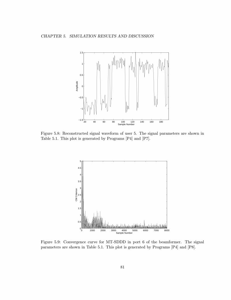
CHAPTER 5. SIMULATION RESULTS AND DISCUSSION
20 40 60 80 100 120 140 160 180−1.5
−1
−0.5
0
0.5
1
1.5
Sample Number
Am
plitu
de
Figure 5.8: Reconstructed signal waveform of user 5. The signal parameters are shown inTable 5.1. This plot is generated by Programs [P4] and [P7].
0 1000 2000 3000 4000 5000 6000 7000 80000
0.5
1
1.5
2
2.5
3
3.5
4
4.5
5
Sample Number
CM
Crit
erio
n
Figure 5.9: Convergence curve for MT-SDDD in port 6 of the beamformer. The signalparameters are shown in Table 5.1. This plot is generated by Programs [P4] and [P8].
81

CHAPTER 5. SIMULATION RESULTS AND DISCUSSION
90◦. The DOA distribution of all the users for both the non-crowded and crowded cases is
illustrated in Figure 5.11. In the following simulation cases, we assume perfect power con-
trol, so all the signals impinging on the array have the same power unless specified otherwise.
Figure 5.12 shows the BER performance of different algorithms for Eb/N0 = 8 dB,
non-crowded DOA case. In Figure 5.12, to generate the BER for the different adaptive
algorithms, we transmit different random bit streams for each user. In the receiver, we use
the beamformer adapted by each algorithm to extract each user’s signal and then feed the
output of the beamformer into the matched filter to despread the signal and estimate the
transmitted data bit. The estimates of the data bits are compared to the original transmit-
ted data bits and the BER of each user is calculated. The BER averaged over all the users
is then calculated and used in the BER performance plot.
From Figure 5.12 we see that the MT-LSCMA cannot work under the low Eb/N0 con-
dition, and its BER performance is very close to that of the conventional receiver. For
the MT-SDDD, when the system is under-loaded (with the number of users less than the
number of antenna elements of the array), the BER increases sharply as the number of
users increases. This is because the MT-SDDD uses the estimate of the data sample as the
desired signal to adapt the weight vectors of the beamformer. When the number of users
increases, the error rate of the data sample estimate becomes larger, and the algorithm
cannot adapt the weight vectors correctly, therefore the improvement due to the spatial fil-
tering becomes smaller and the BER increases. However, comparing the BER performance
of the MT-SDDD with that of the conventional receiver, we see that a large improvement
can still be achieved when the system is under-loaded. When the system is fully-loaded
(with the number of users equal to the number of antenna elements of the array) or over-
loaded (with the number of users greater than the number of antenna elements of the array),
the BER changes smoothly as the number of users increases, and the improvement of the
BER performance over that of the conventional receiver is small. This is because under
82
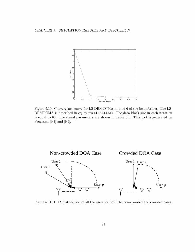
CHAPTER 5. SIMULATION RESULTS AND DISCUSSION
1 1.5 2 2.5 3 3.5 4 4.5 50
0.5
1
1.5
2
2.5
3
3.5
4
Iteration Number
LS
MS
E
Figure 5.10: Convergence curve for LS-DRMTCMA in port 6 of the beamformer. The LS-DRMTCMA is described in equations (4.46)-(4.51). The data block size in each iterationis equal to 60. The signal parameters are shown in Table 5.1. This plot is generated byPrograms [P4] and [P9].
*
*User 1
-700
User 2
*User p
Non-crowded DOA Case
* *User 1 User 2
*User p
Crowded DOA Case
Figure 5.11: DOA distribution of all the users for both the non-crowded and crowded cases.
83

CHAPTER 5. SIMULATION RESULTS AND DISCUSSION
4 5 6 7 8 9 10 11 12 13 1410
−6
10−5
10−4
10−3
10−2
10−1
Number of Users
BE
R
Conv. receiver
MT−LSCMA
MT−SDDD
LS−DRMTA
LS−DRMTCMA
Figure 5.12: BER performance of different adaptive algorithms. In this case, Eb/N0 = 8dB, the DOAs of all the users are equally spaced between −70◦ and 90◦. The ratio of thecoefficients aPN/aCM used in the LS-DRMTCMA is set to 2. This plot is generated byPrograms [P10] and [P12].
4 5 6 7 8 9 10 11 12 13 1410
−6
10−5
10−4
10−3
10−2
10−1
Number of Users
BE
R
Conv. receiver
MT−LSCMA
MT−SDDD
LS−DRMTCMA
LS−DRMTA
Figure 5.13: BER performance of different adaptive algorithms. In this case, Eb/N0 = 8dB, the DOAs of all the users are equally spaced between 0◦ and 90◦. The ratio of thecoefficients aPN/aCM used in the LS-DRMTCMA is set to 2. This plot is generated byPrograms [P10] and [P12].
84
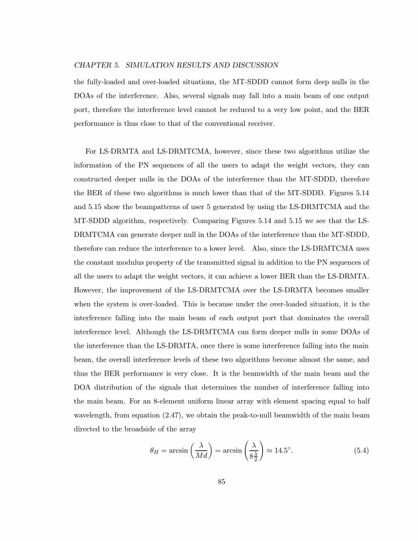
CHAPTER 5. SIMULATION RESULTS AND DISCUSSION
the fully-loaded and over-loaded situations, the MT-SDDD cannot form deep nulls in the
DOAs of the interference. Also, several signals may fall into a main beam of one output
port, therefore the interference level cannot be reduced to a very low point, and the BER
performance is thus close to that of the conventional receiver.
For LS-DRMTA and LS-DRMTCMA, however, since these two algorithms utilize the
information of the PN sequences of all the users to adapt the weight vectors, they can
constructed deeper nulls in the DOAs of the interference than the MT-SDDD, therefore
the BER of these two algorithms is much lower than that of the MT-SDDD. Figures 5.14
and 5.15 show the beampatterns of user 5 generated by using the LS-DRMTCMA and the
MT-SDDD algorithm, respectively. Comparing Figures 5.14 and 5.15 we see that the LS-
DRMTCMA can generate deeper null in the DOAs of the interference than the MT-SDDD,
therefore can reduce the interference to a lower level. Also, since the LS-DRMTCMA uses
the constant modulus property of the transmitted signal in addition to the PN sequences of
all the users to adapt the weight vectors, it can achieve a lower BER than the LS-DRMTA.
However, the improvement of the LS-DRMTCMA over the LS-DRMTA becomes smaller
when the system is over-loaded. This is because under the over-loaded situation, it is the
interference falling into the main beam of each output port that dominates the overall
interference level. Although the LS-DRMTCMA can form deeper nulls in some DOAs of
the interference than the LS-DRMTA, once there is some interference falling into the main
beam, the overall interference levels of these two algorithms become almost the same, and
thus the BER performance is very close. It is the beamwidth of the main beam and the
DOA distribution of the signals that determines the number of interference falling into
the main beam. For an 8-element uniform linear array with element spacing equal to half
wavelength, from equation (2.47), we obtain the peak-to-null beamwidth of the main beam
directed to the broadside of the array
θH = arcsin
(λ
Md
)= arcsin
(λ
8λ2
)≈ 14.5◦. (5.4)
85

CHAPTER 5. SIMULATION RESULTS AND DISCUSSION
−100 −80 −60 −40 −20 0 20 40 60 80 100−50
−45
−40
−35
−30
−25
−20
−15
−10
−5
0
DOA (degrees)
Bea
mpa
ttern
Gai
n (d
B)
Figure 5.14: Beampattern of user 5 generated by using LS-DRMTCMA. In this case,Eb/N0 = 8 dB, the number of users is equal to 8, the DOAs of all the users are equallyspaced between −70◦ and 90◦. The ratio of the coefficients aPN/aCM used in the LS-DRMTCMA is set to 2. This plot is generated by Programs [P4] and [P13].
−100 −80 −60 −40 −20 0 20 40 60 80 100−50
−45
−40
−35
−30
−25
−20
−15
−10
−5
0
DOA (degrees)
Bea
mpa
ttern
Gai
n (d
B)
Figure 5.15: Beampattern of user 5 generated by using MT-SDDD. In this case, Eb/N0 = 8dB, the number of users is equal to 8, the DOAs of all the users are equally spaced between−70◦ and 90◦. The ratio of the coefficients aPN/aCM used in the LS-DRMTCMA is set to2. This plot is generated by Programs [P4] and [P13].
86
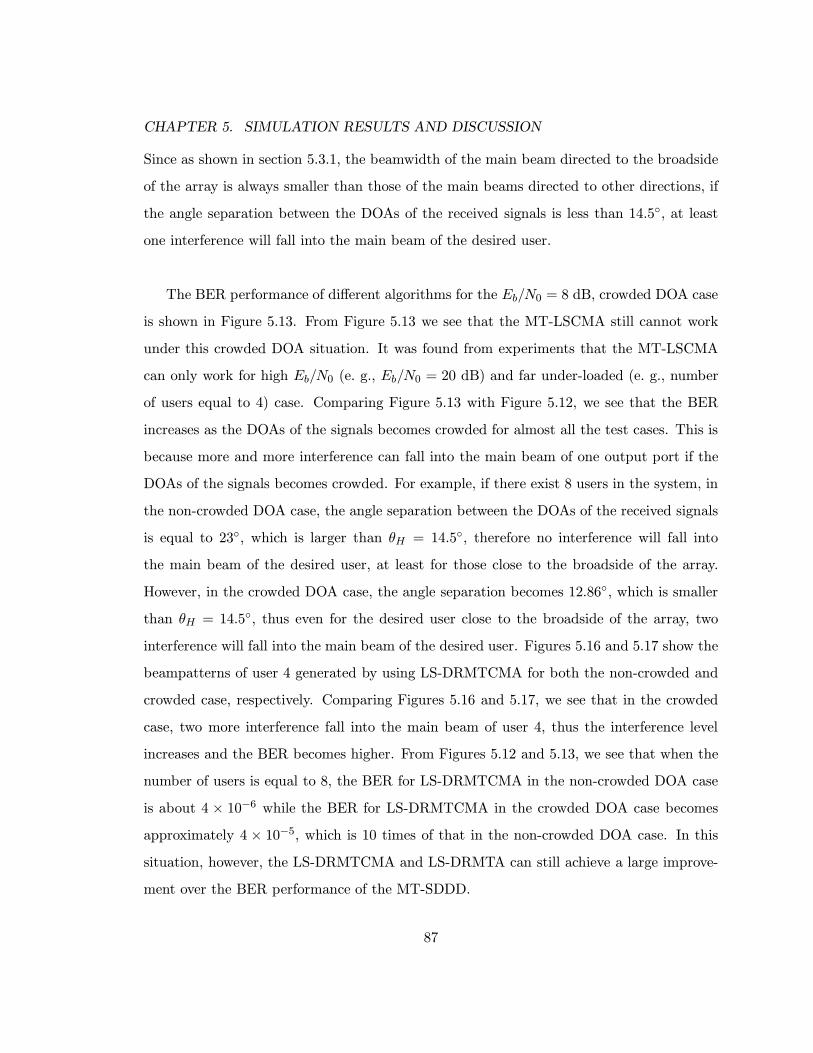
CHAPTER 5. SIMULATION RESULTS AND DISCUSSION
Since as shown in section 5.3.1, the beamwidth of the main beam directed to the broadside
of the array is always smaller than those of the main beams directed to other directions, if
the angle separation between the DOAs of the received signals is less than 14.5◦, at least
one interference will fall into the main beam of the desired user.
The BER performance of different algorithms for the Eb/N0 = 8 dB, crowded DOA case
is shown in Figure 5.13. From Figure 5.13 we see that the MT-LSCMA still cannot work
under this crowded DOA situation. It was found from experiments that the MT-LSCMA
can only work for high Eb/N0 (e. g., Eb/N0 = 20 dB) and far under-loaded (e. g., number
of users equal to 4) case. Comparing Figure 5.13 with Figure 5.12, we see that the BER
increases as the DOAs of the signals becomes crowded for almost all the test cases. This is
because more and more interference can fall into the main beam of one output port if the
DOAs of the signals becomes crowded. For example, if there exist 8 users in the system, in
the non-crowded DOA case, the angle separation between the DOAs of the received signals
is equal to 23◦, which is larger than θH = 14.5◦, therefore no interference will fall into
the main beam of the desired user, at least for those close to the broadside of the array.
However, in the crowded DOA case, the angle separation becomes 12.86◦, which is smaller
than θH = 14.5◦, thus even for the desired user close to the broadside of the array, two
interference will fall into the main beam of the desired user. Figures 5.16 and 5.17 show the
beampatterns of user 4 generated by using LS-DRMTCMA for both the non-crowded and
crowded case, respectively. Comparing Figures 5.16 and 5.17, we see that in the crowded
case, two more interference fall into the main beam of user 4, thus the interference level
increases and the BER becomes higher. From Figures 5.12 and 5.13, we see that when the
number of users is equal to 8, the BER for LS-DRMTCMA in the non-crowded DOA case
is about 4 × 10⁻⁶ while the BER for LS-DRMTCMA in the crowded DOA case becomes
approximately 4 × 10⁻⁵, which is 10 times of that in the non-crowded DOA case. In this
situation, however, the LS-DRMTCMA and LS-DRMTA can still achieve a large improve-
ment over the BER performance of the MT-SDDD.
87

CHAPTER 5. SIMULATION RESULTS AND DISCUSSION
−100 −80 −60 −40 −20 0 20 40 60 80 100−50
−45
−40
−35
−30
−25
−20
−15
−10
−5
0
DOA (degrees)
Bea
mpa
ttern
Gai
n (d
B)
Figure 5.16: Beampattern of user 4 generated by using LS-DRMTCMA. In this case,Eb/N0 = 8 dB, the number of users is equal to 8, the DOAs of all the users are equallyspaced between −70◦ and 90◦. The ratio of the coefficients aPN/aCM used in the LS-DRMTCMA is set to 2. This plot is generated by Programs [P4] and [P13].
−100 −80 −60 −40 −20 0 20 40 60 80 100−50
−45
−40
−35
−30
−25
−20
−15
−10
−5
0
DOA (degrees)
Bea
mpa
ttern
Gai
n (d
B)
Figure 5.17: Beampattern of user 4 generated by using LS-DRMTCMA. In this case,Eb/N0 = 8 dB, the number of users is equal to 8, the DOAs of all the users are equally spacedbetween 0◦ and 90◦. The ratio of the coefficients aPN/aCM used in the LS-DRMTCMA isset to 2. This plot is generated by Programs [P4] and [P13].
88

CHAPTER 5. SIMULATION RESULTS AND DISCUSSION
The BER performance of different algorithms for the Eb/N0 = 4 dB, non-crowded and
crowded DOA cases are shown in Figure 5.18 and Figure 5.19, respectively. Comparing
Figures 5.18 and 5.19 with Figures 5.12 and 5.13, we see that the BER increases as the
Eb/N0 decreases. From Figures 5.18 and 5.19, we see that in the low Eb/N0 case, the LS-
DRMTCMA and LS-DRMTA can still outperform the MT-SDDD for both non-crowded
and crowded DOA cases. Comparing the BER curves of LS-DRMTCMA and LS-DRMTA
in Figures 5.18 and 5.19, we see that the improvement of LS-DRMTCMA over LS-DRMTA
does not degrade very much as the number of users increases, which is different from that in
the Eb/N0 = 8 dB case. This is because for such a low Eb/N0, in addition to the interference,
the noise also plays an important role in determining the BER. Since the difference between
the abilities of the LS-DRMTCMA and LS-DRMTA to reduce the noise changes little as
the number of users increase, the improvement of LS-DRMTCMA over LS-DRMTA does
not degrade very much as the number of users increases. One point to note is that when
the number of users is equal to 4, the BER of the crowded DOA case is less than that of
the non-crowded DOA case. The reason is that when the number of users is equal to 4, the
angle separation between the users is large for both the crowded and non-crowded DOA
cases, so there is no interference falling into the main beam near the broadside of the array,
and only the users near the endfire of the array can affect each other. The beampattern of
user 4 which is near the endfire of the array for both the non-crowded and crowded cases are
illustrated in Figures 5.20 and 5.21, respectively. For the crowded DOA case, the DOAs of
the signals are equally spaced between 0◦ and 90◦, so there is only one user near the endfire
of the array. For the non-crowded case, on the other hand, the DOAs of the signals are
equally spaced between −70◦ and 90◦, thus there are two users near the endfire of the array
and they interference with each other, which results in a higher BER than in the crowded
DOA case.
89

CHAPTER 5. SIMULATION RESULTS AND DISCUSSION
4 5 6 7 8 9 10 11 12 13 1410
−6
10−5
10−4
10−3
10−2
10−1
Number of Users
BE
R
Conv. receiver
MT−LSCMA
MT−SDDD
LS−DRMTA
LS−DRMTCMA
Figure 5.18: BER performance of different adaptive algorithms. In this case, Eb/N0 = 4dB, the DOAs of all the users are equally spaced between −70◦ and 90◦. The ratio of thecoefficients aPN/aCM used in the LS-DRMTCMA is set to 2. This plot is generated byPrograms [P10] and [P12].
4 5 6 7 8 9 10 11 12 13 1410
−6
10−5
10−4
10−3
10−2
10−1
Number of Users
BE
R
Conv. receiver
MT−LSCMA
MT−SDDD
LS−DRMTA
LS−DRMTCMA
Figure 5.19: BER performance of different adaptive algorithms. In this case, Eb/N0 = 4dB, the DOAs of all the users are equally spaced between 0◦ and 90◦. The ratio of thecoefficients aPN/aCM used in the LS-DRMTCMA is set to 2. This plot is generated byPrograms [P10] and [P12].
90
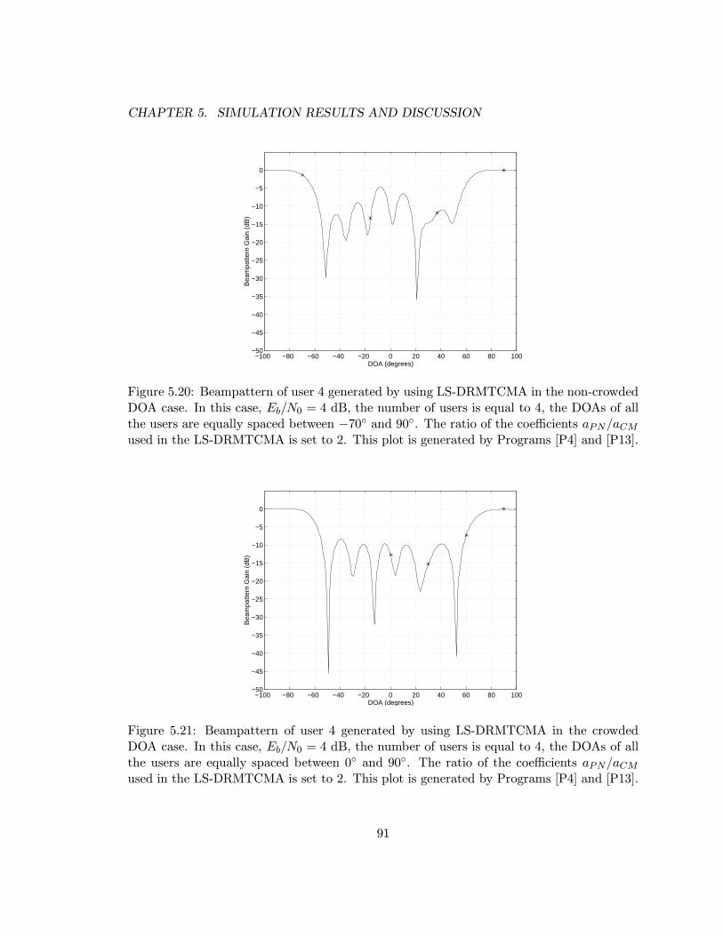
CHAPTER 5. SIMULATION RESULTS AND DISCUSSION
−100 −80 −60 −40 −20 0 20 40 60 80 100−50
−45
−40
−35
−30
−25
−20
−15
−10
−5
0
DOA (degrees)
Bea
mpa
ttern
Gai
n (d
B)
Figure 5.20: Beampattern of user 4 generated by using LS-DRMTCMA in the non-crowdedDOA case. In this case, Eb/N0 = 4 dB, the number of users is equal to 4, the DOAs of allthe users are equally spaced between −70◦ and 90◦. The ratio of the coefficients aPN/aCMused in the LS-DRMTCMA is set to 2. This plot is generated by Programs [P4] and [P13].
−100 −80 −60 −40 −20 0 20 40 60 80 100−50
−45
−40
−35
−30
−25
−20
−15
−10
−5
0
DOA (degrees)
Bea
mpa
ttern
Gai
n (d
B)
Figure 5.21: Beampattern of user 4 generated by using LS-DRMTCMA in the crowdedDOA case. In this case, Eb/N0 = 4 dB, the number of users is equal to 4, the DOAs of allthe users are equally spaced between 0◦ and 90◦. The ratio of the coefficients aPN/aCMused in the LS-DRMTCMA is set to 2. This plot is generated by Programs [P4] and [P13].
91

CHAPTER 5. SIMULATION RESULTS AND DISCUSSION
5.4 BER Performance in Timing Offset Case
In a CDMA system, due to the low SNR and high interference level, the synchronization
of the PN sequence in the receiver cannot be performed perfectly, therefore a timing offset
To exists between the local generated PN sequence and the received PN sequence. This
timing offset will degrade the performance of the system. In this section, we will examine
the BER performance of all the algorithms under different timing offset conditions. We will
consider two timing offset cases, To = 0.25Tc, and To = 0.5Tc, where Tc is the chip period
of the CDMA signal. For each timing offset case, we will also consider two different DOA
distribution cases, the non-crowded DOA case, and the crowded DOA case.
The BER performance of different algorithms for To = 0.25Tc in both non-crowded
and crowded DOA cases are shown in Figures 5.22 and 5.23, respectively. Comparing Fig-
ures 5.22 and 5.23 with Figures 5.12 and 5.13, we see that the BER performance of all the
algorithms in both the non-crowded and crowded DOA cases is degraded due to the timing
offset between the local generated PN sequence and the received PN sequence. However,
comparing the BER curves of LS-DRMTCMA and LS-DRMTA with that of the MT-SDDD,
we see that a big improvement can still be achieved by using the LS-DRMTCMA and LS-
DRMTA in this timing offset case. Also, we see that the LS-DRMTCMA outperforms
the LS-DRMTA. Comparing Figure 5.22 with Figure 5.23, we note that the BER in the
crowded DOA case is higher than that in the non-crowded DOA case for almost all the test
cases, except for the case where the number of users is equal to 4. The reason for this has
been explained in section 5.3.2.
The BER performance of different algorithms for To = 0.5Tc in both non-crowded and
crowded DOA cases is shown in Figures 5.24 and 5.25, respectively. From Figures 5.24 and
5.25 we can see that the improvement of LS-DRMTCMA and LS-DRMTA over the MT-
SDDD becomes very small. The reason is that the BER in this case is now mainly caused
92

CHAPTER 5. SIMULATION RESULTS AND DISCUSSION
4 5 6 7 8 9 10 11 12 13 1410
−6
10−5
10−4
10−3
10−2
10−1
100
Number of Users
BE
R
Conv. receiver
MT−LSCMA
MT−SDDD
LS−DRMTA
LS−DRMTCMA
Figure 5.22: BER performance of different adaptive algorithms in timing offset case. Inthis case, Eb/N0 = 8 dB, To = 0.25Tc, the DOAs of all the users are equally spaced between−70◦ and 90◦. The ratio of the coefficients aPN/aCM used in the LS-DRMTCMA is set to2. This plot is generated by Programs [P14] and [P15].
4 5 6 7 8 9 10 11 12 13 1410
−6
10−5
10−4
10−3
10−2
10−1
100
Number of Users
BE
R
Conv. receiver
MT−SDDD
LS−DRMTA
LS−DRMTCMA
MT−LSCMA
Figure 5.23: BER performance of different adaptive algorithms in timing offset case. Inthis case, Eb/N0 = 8 dB, To = 0.25Tc, the DOAs of all the users are equally spaced between0◦ and 90◦. The ratio of the coefficients aPN/aCM used in the LS-DRMTCMA is set to 2.This plot is generated by Programs [P14] and [P15].
93
CHAPTER 5. SIMULATION RESULTS AND DISCUSSION
by the timing offset, and the spatial filtering has little effect on the BER performance.
The BER vs. the timing offset for both the non-crowded and crowded DOA cases are
shown in Figures 5.26 and 5.27, respectively. In Figures 5.26 and 5.27, the number of users is
equal to 10, and the Eb/N0 is equal to 8 dB. From Figures 5.26 and 5.27 we see that the BER
of all the algorithms rises as the timing offset increases. When To ≤ 0.3Tc, the improvement
of LS-DRMTCMA and LS-DRMTA over other algorithms is large, but this improvement
decreases as the timing offset increases and the BER is dominated by the timing offset.
Therefore, if we can use the conventional receiver to perform the synchronization of the PN
sequence and reduce the timing offset to 0.3Tc, we can then use the beamformer adapted
by the LS-DRMTCMA to extract the signal, and the output of the beamformer can again
be used in the synchronization. Since the beamformer has rejected most of the interference,
the synchronization can be performed more accurately using the beamformer output, and
the smaller timing offset in turn can result in more improvement due to spatial filtering.
5.5 BER Performance in Frequency Offset Case
In a CDMA system, a frequency offset Fo may exist between the local oscillator output
and the carrier of the signals impinging on the array due to the variation of the electronic
components in the local oscillator. This frequency offset will cause a time-varying phase
shift between the base-band signal in the receiver and that in the transmitter. If this
frequency offset cannot be compensated in the receiver, the BER performance will be de-
graded. In this section, we will examine the BER performance of all the algorithms under
different frequency offset conditions. We will consider two frequency offset cases, Fo = 100
Hz, and Fo = 500 Hz. For each frequency offset case, we will also consider two different
DOA distribution cases, the non-crowded DOA case, and the crowded DOA case.
Since a phase shift in the received signal will cause a rotation of the received signal
94

CHAPTER 5. SIMULATION RESULTS AND DISCUSSION
4 5 6 7 8 9 10 11 12 13 1410
−3
10−2
10−1
100
Number of Users
BE
R
Conv. receiver
MT−LSCMA
MT−SDDD
LS−DRMTA
LS−DRMTCMA
Figure 5.24: BER performance of different adaptive algorithms in timing offset case. Inthis case, Eb/N0 = 8 dB, To = 0.5Tc, the DOAs of all the users are equally spaced between−70◦ and 90◦. The ratio of the coefficients aPN/aCM used in the LS-DRMTCMA is set to2. This plot is generated by Programs [P14] and [P16].
4 5 6 7 8 9 10 11 12 13 1410
−3
10−2
10−1
100
Number of Users
BE
R
Conv. receiver
MT−LSCMA
MT−SDDD
LS−DRMTA
LS−DRMTCMA
Figure 5.25: BER performance of different adaptive algorithms in timing offset case. Inthis case, Eb/N0 = 8 dB, To = 0.5Tc, the DOAs of all the users are equally spaced between0◦ and 90◦. The ratio of the coefficients aPN/aCM used in the LS-DRMTCMA is set to 2.This plot is generated by Programs [P14] and [P16].
95

CHAPTER 5. SIMULATION RESULTS AND DISCUSSION
0 0.1 0.2 0.3 0.4 0.5 0.6 0.7 0.8 0.9 110
−4
10−3
10−2
10−1
100
Timing Offset (Tc)
BE
R
Conv. receiver
MT−LSCMA
MT−SDDD
LS−DRMTA
LS−DRMTCMA
Figure 5.26: BER vs. timing offset for different adaptive algorithms. In this case, Eb/N0 = 8dB, the number of users is equal to 10, the DOAs of all the users are equally spaced between−70◦ and 90◦. The ratio of the coefficients aPN/aCM used in the LS-DRMTCMA is set to2. This plot is generated by Programs [P14] and [P17].
0 0.1 0.2 0.3 0.4 0.5 0.6 0.7 0.8 0.9 110
−4
10−3
10−2
10−1
100
Timing Offset (Tc)
BE
R
Conv. receiver
MT−LSCMA
LS−DRMTA
LS−DRMTCMA
MT−SDDD
Figure 5.27: BER vs. timing offset for different adaptive algorithms. In this case, Eb/N0 = 8dB, the number of users is equal to 10, the DOAs of all the users are equally spaced between0◦ and 90◦. The ratio of the coefficients aPN/aCM used in the LS-DRMTCMA is set to 2.This plot is generated by Programs [P14] and [P17].
96
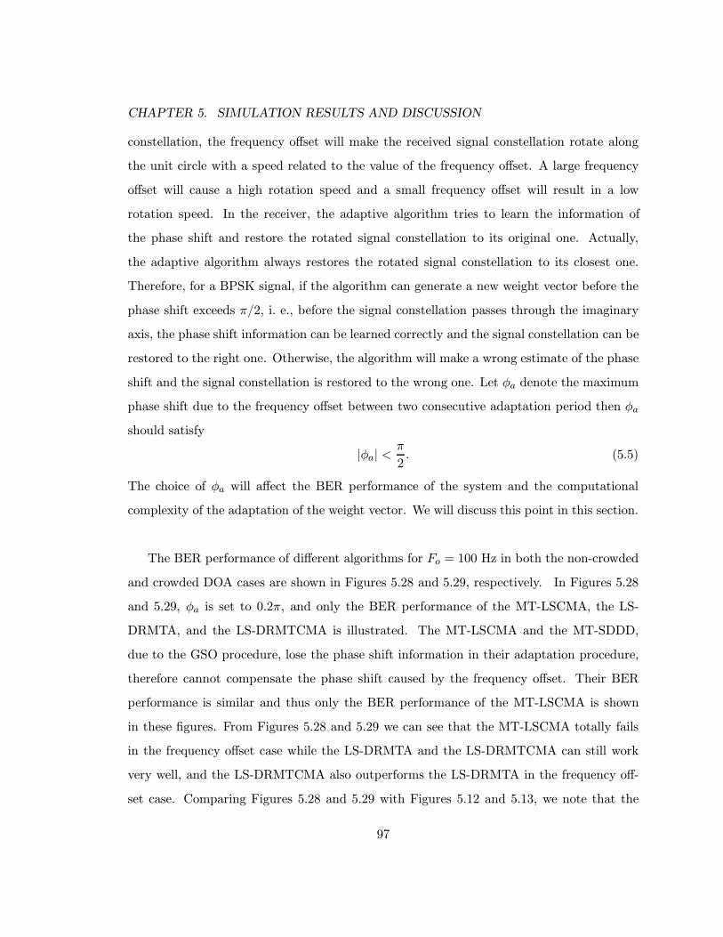
CHAPTER 5. SIMULATION RESULTS AND DISCUSSION
constellation, the frequency offset will make the received signal constellation rotate along
the unit circle with a speed related to the value of the frequency offset. A large frequency
offset will cause a high rotation speed and a small frequency offset will result in a low
rotation speed. In the receiver, the adaptive algorithm tries to learn the information of
the phase shift and restore the rotated signal constellation to its original one. Actually,
the adaptive algorithm always restores the rotated signal constellation to its closest one.
Therefore, for a BPSK signal, if the algorithm can generate a new weight vector before the
phase shift exceeds π/2, i. e., before the signal constellation passes through the imaginary
axis, the phase shift information can be learned correctly and the signal constellation can be
restored to the right one. Otherwise, the algorithm will make a wrong estimate of the phase
shift and the signal constellation is restored to the wrong one. Let φa denote the maximum
phase shift due to the frequency offset between two consecutive adaptation period then φa
should satisfy
|φa| <π
2. (5.5)
The choice of φa will affect the BER performance of the system and the computational
complexity of the adaptation of the weight vector. We will discuss this point in this section.
The BER performance of different algorithms for Fo = 100 Hz in both the non-crowded
and crowded DOA cases are shown in Figures 5.28 and 5.29, respectively. In Figures 5.28
and 5.29, φa is set to 0.2π, and only the BER performance of the MT-LSCMA, the LS-
DRMTA, and the LS-DRMTCMA is illustrated. The MT-LSCMA and the MT-SDDD,
due to the GSO procedure, lose the phase shift information in their adaptation procedure,
therefore cannot compensate the phase shift caused by the frequency offset. Their BER
performance is similar and thus only the BER performance of the MT-LSCMA is shown
in these figures. From Figures 5.28 and 5.29 we can see that the MT-LSCMA totally fails
in the frequency offset case while the LS-DRMTA and the LS-DRMTCMA can still work
very well, and the LS-DRMTCMA also outperforms the LS-DRMTA in the frequency off-
set case. Comparing Figures 5.28 and 5.29 with Figures 5.12 and 5.13, we note that the
97

CHAPTER 5. SIMULATION RESULTS AND DISCUSSION
4 5 6 7 8 9 10 11 12 13 1410
−6
10−5
10−4
10−3
10−2
10−1
100
Number of Users
BE
R
MT−LSCMA
LS−DRMTA
LS−DRMTCMA
Figure 5.28: BER performance of different adaptive algorithms in frequency offset case. Inthis case, Eb/N0 = 8 dB, Fo = 100 Hz, the DOAs of all the users are equally spaced between−70◦ and 90◦. The ratio of the coefficients aPN/aCM used in the LS-DRMTCMA is set to2. The maximum phase shift φa between two consecutive adaptation period is set to 0.2π.This plot is generated by Programs [P18] and [P19].
4 5 6 7 8 9 10 11 12 13 1410
−6
10−5
10−4
10−3
10−2
10−1
100
Number of Users
BE
R
MT−LSCMA
LS−DRMTA
LS−DRMTCMA
Figure 5.29: BER performance of different adaptive algorithms in frequency offset case. Inthis case, Eb/N0 = 8 dB, Fo = 100 Hz, the DOAs of all the users are equally spaced between0◦ and 90◦. The ratio of the coefficients aPN/aCM used in the LS-DRMTCMA is set to2. The maximum phase shift φa between two consecutive adaptation period is set to 0.2π.This plot is generated by Programs [P18] and [P19].
98

CHAPTER 5. SIMULATION RESULTS AND DISCUSSION
BER performance of all the algorithms in both the non-crowded and crowded DOA cases is
degraded due to the frequency offset. Comparing Figure 5.28 with Figure 5.29, we can see
that the BER in crowded DOA case is higher than that in the non-crowded DOA case for
almost all the test cases, except for the case where the number of users is equal to 4. This
phenomenon is the same as that shown in the timing offset case.
The BER performance of different algorithms for Fo = 500 Hz in both the non-crowded
and crowded DOA cases is illustrated in Figures 5.30 and 5.31, respectively. Comparing
Figures 5.30 and 5.31 with Figures 5.28 and 5.29, we see that the BERs of both algorithms
change little as the frequency offset increases. Figure 5.32 shows the BER vs. frequency
offset for all the algorithm with the number of users equal to 10. In Figure 5.32, the DOAs
of all the users are equally spaced between −60◦ and 60◦, and φa is set to 0.2π. From
Figure 5.32 we see that for LS-DRMTA and LS-DRMTCMA, the BER performance is al-
most independent of the frequency offset, which indicates that the phase shift caused by
the frequency offset is indeed compensated by the algorithms.
Figure 5.33 shows the BER vs. frequency offset for LS-DRMTA and LS-DRMTCMA
with different φa. From Figure 5.33 we see that by reducing φa, we can get a lower BER.
However, since a smaller φa means a short adaptation period, this small improvement is
paid by a higher computational complexity of the adaptation of the weight vectors. There
is a trade-off between the BER performance and φa (i. e., the computational complexity
of the adaptation). Figure 5.34 shows the BER vs. φa for different frequency offset using
LS-DRMTA. The same plot for LS-DRMTCMA is illustrated in Figure 5.35. From Fig-
ures 5.34 and 5.35 we can see that when φa ≤ 0.2π, the BER curves are flat, and increasing
φa only result in a small degradation of the BER performance. However, once φa > 0.2π,
increasing φa will cause larger degradation of the BER performance. Therefore, 0.2π is the
optimum value for φa.
99
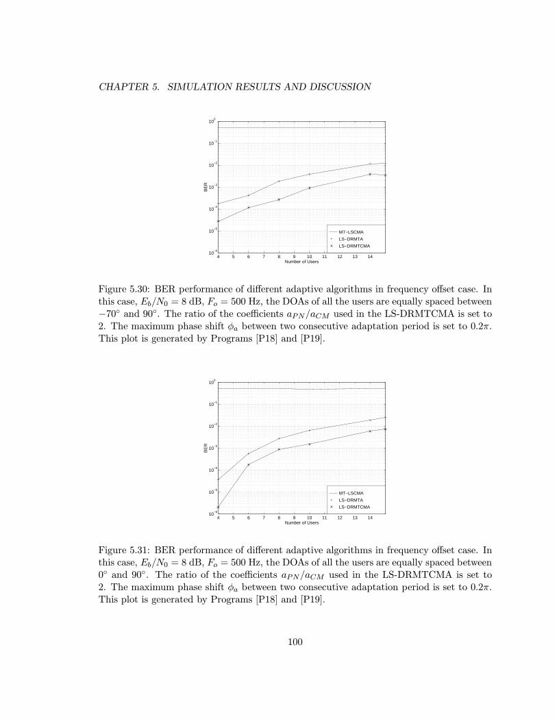
CHAPTER 5. SIMULATION RESULTS AND DISCUSSION
4 5 6 7 8 9 10 11 12 13 1410
−6
10−5
10−4
10−3
10−2
10−1
100
Number of Users
BE
R
MT−LSCMA
LS−DRMTA
LS−DRMTCMA
Figure 5.30: BER performance of different adaptive algorithms in frequency offset case. Inthis case, Eb/N0 = 8 dB, Fo = 500 Hz, the DOAs of all the users are equally spaced between−70◦ and 90◦. The ratio of the coefficients aPN/aCM used in the LS-DRMTCMA is set to2. The maximum phase shift φa between two consecutive adaptation period is set to 0.2π.This plot is generated by Programs [P18] and [P19].
4 5 6 7 8 9 10 11 12 13 1410
−6
10−5
10−4
10−3
10−2
10−1
100
Number of Users
BE
R
MT−LSCMA
LS−DRMTA
LS−DRMTCMA
Figure 5.31: BER performance of different adaptive algorithms in frequency offset case. Inthis case, Eb/N0 = 8 dB, Fo = 500 Hz, the DOAs of all the users are equally spaced between0◦ and 90◦. The ratio of the coefficients aPN/aCM used in the LS-DRMTCMA is set to2. The maximum phase shift φa between two consecutive adaptation period is set to 0.2π.This plot is generated by Programs [P18] and [P19].
100

CHAPTER 5. SIMULATION RESULTS AND DISCUSSION
0 50 100 150 200 250 300 350 400 450 50010
−6
10−5
10−4
10−3
10−2
10−1
100
Frequency Offset (Hz)
BE
R
MT−LSCMA
MT−SDDD
LS−DRMTA
LS−DRMTCMA
Figure 5.32: BER vs. frequency offset for different adaptive algorithms. In this case,Eb/N0 = 8 dB, the number of users is equal to 10, the DOAs of all the users are equallyspaced between −60◦ and 60◦. The ratio of the coefficients aPN/aCM used in the LS-DRMTCMA is set to 2. The maximum phase shift φa between two consecutive adaptationperiod is set to 0.2π. This plot is generated by Programs [P18] and [P20].
0 50 100 150 200 250 300 350 400 450 50010
−6
10−5
10−4
10−3
10−2
10−1
100
Frequency Offset (Hz)
BE
R
LS−DRMTA, max. phase shift = 0.2*pi
LS−DRMTCMA, max. phase shift = 0.2*pi
LS−DRMTA, max. phase shift = 0.05*pi
LS−DRMTCMA, max. phase shift = 0.05*pi
Figure 5.33: BER vs. frequency offset for different adaptive algorithms with different φa.In this case, Eb/N0 = 8 dB, the number of users is equal to 10, the DOAs of all the usersare equally spaced between −60◦ and 60◦. The ratio of the coefficients aPN/aCM used inthe LS-DRMTCMA is set to 2. This plot is generated by Programs [P18] and [P21].
101

CHAPTER 5. SIMULATION RESULTS AND DISCUSSION
0.05 0.1 0.15 0.2 0.25 0.3 0.35 0.4 0.4510
−6
10−5
10−4
10−3
10−2
10−1
100
Maximum Phase−shift (pi)
BE
R
Freq. offset = 100 HzFreq. offset = 500 Hz
Figure 5.34: BER vs. φa for different frequency offset using LS-DRMTA. In this case,Eb/N0 = 8 dB, the number of users is equal to 10, the DOAs of all the users are equallyspaced between −60◦ and 60◦. This plot is generated by Programs [P18] and [P22].
0.05 0.1 0.15 0.2 0.25 0.3 0.35 0.4 0.4510
−6
10−5
10−4
10−3
10−2
10−1
100
Maximum Phase−shift (pi)
BE
R
Freq. offset = 100 HzFreq. offset = 500 Hz
Figure 5.35: BER vs. φa for different frequency offset using LS-DRMTCMA. In this case,Eb/N0 = 8 dB, the number of users is equal to 10, the DOAs of all the users are equallyspaced between −60◦ and 60◦. The ratio of the coefficients aPN/aCM used in the LS-DRMTCMA is set to 2. This plot is generated by Programs [P18] and [P22].
102

CHAPTER 5. SIMULATION RESULTS AND DISCUSSION
In all the above simulation cases for LS-DRMTA and LS-DRMTCMA, we assume that
the random phase of each signal impinging on the array is known and is compensated before
the signal is used in the algorithms. However, the LS-DRMTA and the LS-DRMTCMA
can also work without this phase information. Figure 5.36 shows the BER performance
of different adaptive algorithms for Fo = 100 Hz without phase information. Comparing
Figure 5.36 with Figure 5.28, we see that without the phase information, the LS-DRMTA
and LS-DRMTCMA can still achieve almost the same BER performance as that with the
phase information.
4 5 6 7 8 9 10 11 12 13 1410
−6
10−5
10−4
10−3
10−2
10−1
100
Number of Users
BE
R
MT−LSCMA w/o phase inf.
LS−DRMTA w/o phase inf.
LS−DRMTCMA w/o phase inf.
Figure 5.36: BER performance of different adaptive algorithms in frequency offset casewithout phase information. In this case, Eb/N0 = 8 dB, Fo = 100 Hz, the DOAs of all theusers are equally spaced between −70◦ and 90◦. The ratio of the coefficients aPN/aCM usedin the LS-DRMTCMA is set to 2. The maximum phase shift φa between two consecutiveadaptation period is set to 0.2π. This plot is generated by Programs [P18] and [P23].
5.6 BER Performance and Coefficients in LS-DRMTCMA
In the above simulation cases, the ratio of aPN to aCM in the LS-DRMTCMA is always
set to 2. In this section, we will examine the effect of varying aPN/aCM on the BER per-
formance of LS-DRMTCMA.
103

CHAPTER 5. SIMULATION RESULTS AND DISCUSSION
Figure 5.37 shows the BER vs. aPN/aCM for the LS-DRMTCMA in different simulation
environments. From Figure 5.37 we see that without timing offset and frequency offset,
the LS-DRMTCMA can always achieve the best BER performance when aPN/aCM = 0.5
no matter what the number of users is and what the Eb/N0 will be. For the case with
timing offset and frequency offset, although the BER performance is not the best when
aPN/aCM = 0.5, the difference between the best BER performance and that obtained at
the point where aPN/aCM = 0.5 is very small. Therefore it is recommended that aPN/aCM
should be set to 0.5 for LS-DRMTCMA to obtain the best BER performance. In Fig-
ure 5.37, the points where aPN/aCM = 100 are actually corresponding to the LS-DRMTA,
and we see that the LS-DRMTCMA with aPN/aCM = 0.5 can achieve a large improvement
over the LS-DRMTA.
Someone may ask if the improvement obtained by varying the term aPN/aCM may have
resulted from the fact that the algorithm may not fully converge when the aPN/aCM is
changed. Figure 5.38 shows the BER vs. aPN/aCM for LS-DRMTCMA with different itera-
tion number. From Figure 5.38 we see that although we have increased the iteration number
from 5 to 8, the BER performance changes little, and the point where aPN/aCM = 0.5 is
still a local minimum of the BER curve. Thus we can conclude that the LS-DRMTCMA
can fully converge with 5 iterations for different aPN/aCM value, and 0.5 is the optimum
value of aPN/aCM for LS-DRMTCMA to achieve the best BER performance.
5.7 BER Performance in Multipath Environment
In a wireless radio channel, the transmitted signal may arrive at the receiver through
different paths with different time delays. These multipath will cause the intersymbol inter-
ference (ISI) and degrade the BER performance of the system. However, if these multipaths
are coming from different DOAs, we can use an adaptive array in the receiver to extract
104

CHAPTER 5. SIMULATION RESULTS AND DISCUSSION
10−2
10−1
100
101
102
10−7
10−6
10−5
10−4
10−3
10−2
10−1
100
a_PN/a_CM
BE
R
10 users, Eb/No = 8 dB, To = 0, Fo = 0
10 users, Eb/No = 4 dB, To = 0, Fo = 0
8 users, Eb/No = 4 dB, To = 0, Fo = 0
10 users, Eb/No = 8 dB, To = 0.25*Tc, Fo = 0
10 users, Eb/No = 8 dB, To = 0, Fo = 100 Hz
Figure 5.37: BER vs. aPN/aCM for LS-DRMTCMA in different simulation environments.The DOAs of all the users are equally spaced between −70◦ and 90◦. For frequency offsetcase, the maximum phase shift φa between two consecutive adaptation period is set to 0.2π.This plot is generated by Programs [P24] and [P25].
10−2
10−1
100
101
102
10−7
10−6
10−5
10−4
10−3
10−2
10−1
100
a_PN/a_CM
BE
R
5 iterations8 iterations
Figure 5.38: BER vs. aPN/aCM for LS-DRMTCMA with different iteration number. Inthis case, Eb/N0 = 8 dB, the number of users is equal to 10, the DOAs of all the users areequally spaced between −70◦ and 90◦. There is no timing offset and frequency offset. Thisplot is generated by Programs [P24] and [P26].
105

CHAPTER 5. SIMULATION RESULTS AND DISCUSSION
the path with the strongest power and reject the other ones, therefore reducing the ISI and
improving the BER performance. In this section, we will examine the BER performance of
different algorithms in the multipath environment.
The channel model we use in the simulation is the 2-ray resolvable channel where each
user has two multipaths. The reason for using the 2-ray resolvable channel is that the
bandwidth of the transmitted signal, i. e., the direct sequence spread spectrum signal, is
very high compared to the bandwidth of the wireless radio channel, therefore the multipaths
are resolvable in time. The first issue we need to consider for the channel model is the DOAs
of the multipaths. In the 2-ray channel model, the two multipaths have different DOAs, and
we want to investigate the effect of varying the angle separation between the multipaths
on the performance of different algorithms. In the simulation, we consider two different
multipath angle separation cases. In the first case, the DOA difference between the two
multipaths is set to 10◦ while in the second case, the DOA difference is set to 20◦. As shown
in section 5.3.2, for an 8-element uniform linear array with element spacing equal to half
wavelength, the peak-to-null beamwidth, θH , of the main beam directed to the broadside
of the array is approximately equal to 14.5◦. By setting the multipath angle separation
equal to 10◦ and 20◦, which are less and greater than θH , respectively, we can investigate
the performance of different algorithms under the condition when both multipaths fall into
the main beam and the condition when only one multipath fall into the main beam. The
second issue we need to consider for the channel model is the time delay between the two
multipaths. For different multipath angle separation cases, the time delay between the two
multipaths should be varied . It was shown in [56] and [57] that the time delay between
the multipaths with close DOAs tend to be small and that between the multipaths with
far separated DOAs tend to be large. Since we also want to investigate the performance of
different algorithms under the condition when the time delay between the two multipaths
is less and greater than the chip period Tc, for the first case with small DOA difference, we
set the time delay between the two multipaths to 0.5Tc while for the second case with large
106

CHAPTER 5. SIMULATION RESULTS AND DISCUSSION
DOA difference, we set the time delay between the two multipaths to 1.5Tc. The last issue
we need to consider for the channel model is the power ratio between the two multipaths.
As shown in [58], the amplitude of each single multipath varies little over a small range of
distance. Also, since the data bit rate of the system is very high (128kbps), we will consider
the amplitude of each multipath unchanged over the simulation period. In the simulation,
we want to investigate the effect of varying the power ratio between the multipaths on the
performance of different algorithms. So three different power ratios of the first path to the
second path, 0 dB, 6dB, and 10dB, are considered for each multipath angle separation case.
The signal parameters of the multipaths in different simulation cases are shown in Table 5.2.
Table 5.2: Signal Parameters of Multipaths
Case #DOA Difference Time Delay Power Ratio (dB)
Between Multipaths Between Multipaths (First Path/Second Path)
1 10◦ 0.5Tc 0
2 10◦ 0.5Tc 6
3 10◦ 0.5Tc 10
4 20◦ 1.5Tc 0
5 20◦ 1.5Tc 6
6 20◦ 1.5Tc 10
The BER performance of different algorithms for simulation case 1, 2 and 3 are illus-
trated in Figures 5.39, 5.40, and 5.41, respectively. Comparing Figures 5.39, 5.40, and 5.41
with Figure 5.12, we see that the BER performance is indeed degraded by the multipath in
all the cases. Comparing Figures 5.39, 5.40, and 5.41, we note that decreasing the power
ratio between the multipaths will result in a higher BER. This is what we expect since in
these three simulation cases, the angle separation between the multipaths is equal to 10◦,
which is less than θH = 14.5◦, hence both of the multipaths fall into the main beam of
the output port, and a lower power ratio between the multipaths means a higher ISI level,
which will result in a worse BER performance. However, from Figures 5.39, 5.40, and 5.41,
107

CHAPTER 5. SIMULATION RESULTS AND DISCUSSION
we see that even for such a small multipath angle separation, using the adaptive array in the
receiver can still reduce the multipath effect and improve the BER performance, although
the improvement becomes smaller when the power ratio between the multipaths decreases.
Also note that the LS-DRMTCMA with aPN/aCM = 0.5 can achieve a large improvement
over that with aPN/aCM = 2 for all the simulation cases. This has confirmed the conclusion
we draw in section 5.6.
The BER performance of different algorithms for simulation case 4, 5 and 6 are illus-
trated in Figures 5.42, 5.43, and 5.44, respectively. From Figures 5.42, 5.43, and 5.44, we
see that although the angle separation between the multipaths is now equal to 20◦, which
is greater than θH = 14.5◦, as in the close multipath DOA case, decreasing the power ratio
between the multipaths will also result in a higher BER. The reason is that the beamformer
cannot ideally form a null in the direction of the second path, so decreasing the power ratio
between the multipaths still will result in a higher ISI level. Also since the angle separation
is now equal to 20◦, the multipaths of one user may fall into the main beam constructed
for another user, hence decreasing the power ratio between the multipaths will increase the
interference level of the desired user. The higher ISI and interference level will then cause
a worse BER performance. Comparing Figures 5.42, 5.43, and 5.44 with Figures 5.39, 5.40,
and 5.41, we see that the BER of the well-separated multipath DOA case is lower than
that of the close multipath DOA case, and the improvement obtained by using the adaptive
array is larger in the well-separated DOA case. The reason is that in the close DOA case
where the DOAs of the multipaths are separated by only 10◦, all the multipaths tend to
fall into the main beam of the output port, and thus the adaptive array cannot rejected
the multipath effectively. However, in the well-separated multipath DOA case, for most of
the users, only one multipath can fall into the main beam of the output port, therefore the
multipath effect can be reduced by the array to a very low level.
108

CHAPTER 5. SIMULATION RESULTS AND DISCUSSION
4 5 6 7 8 9 10 11 12 13 1410
−7
10−6
10−5
10−4
10−3
10−2
10−1
100
Number of Users
BE
RConv. receiver
MT−SDDD
LS−DRMTA
LS−DRMTCMA, a_PN/a_CM = 2
LS−DRMTCMA, a_PN/a_CM = 0.5
Figure 5.39: BER performance of different adaptive algorithms in multipath environment.In this case, Eb/N0 = 8 dB, the DOAs of the first paths of all the users are equally spacedbetween −70◦ and 90◦. The DOA of the second path is 10◦ less than that of the first path.The power ratio of the first path to the second path is 0 dB, and the time delay betweenthese two paths is 0.5Tc. This plot is generated by Programs [P27] and [P29].
4 5 6 7 8 9 10 11 12 13 1410
−7
10−6
10−5
10−4
10−3
10−2
10−1
100
Number of Users
BE
R
Conv. receiver
MT−SDDD
LS−DRMTA
LS−DRMTCMA, a_PN/a_CM = 2
LS−DRMTCMA, a_PN/a_CM = 0.5
Figure 5.40: BER performance of different adaptive algorithms in multipath environment.In this case, Eb/N0 = 8 dB, the DOAs of the first paths of all the users are equally spacedbetween −70◦ and 90◦. The DOA of the second path is 10◦ less than that of the first path.The power ratio of the first path to the second path is 6 dB, and the time delay betweenthese two paths is 0.5Tc. This plot is generated by Programs [P27] and [P29].
109

CHAPTER 5. SIMULATION RESULTS AND DISCUSSION
4 5 6 7 8 9 10 11 12 13 1410
−7
10−6
10−5
10−4
10−3
10−2
10−1
100
Number of Users
BE
RConv. receiver
MT−SDDD
LS−DRMTA
LS−DRMTCMA, a_PN/a_CM = 2
LS−DRMTCMA, a_PN/a_CM = 0.5
Figure 5.41: BER performance of different adaptive algorithms in multipath environment.In this case, Eb/N0 = 8 dB, the DOAs of the first paths of all the users are equally spacedbetween −70◦ and 90◦. The DOA of the second path is 10◦ less than that of the first path.The power ratio of the first path to the second path is 10 dB, and the time delay betweenthese two paths is 0.5Tc. This plot is generated by Programs [P27] and [P29].
4 5 6 7 8 9 10 11 12 13 1410
−7
10−6
10−5
10−4
10−3
10−2
10−1
100
Number of Users
BE
R
Conv. receiver
MT−SDDD
LS−DRMTA
LS−DRMTCMA, a_PN/a_CM = 2
LS−DRMTCMA, a_PN/a_CM = 0.5
Figure 5.42: BER performance of different adaptive algorithms in multipath environment.In this case, Eb/N0 = 8 dB, the DOAs of the first paths of all the users are equally spacedbetween −70◦ and 90◦. The DOA of the second path is 20◦ less than that of the first path.The power ratio of the first path to the second path is 0 dB, and the time delay betweenthese two paths is 1.5Tc. This plot is generated by Programs [P28] and [P29].
110

CHAPTER 5. SIMULATION RESULTS AND DISCUSSION
4 5 6 7 8 9 10 11 12 13 1410
−7
10−6
10−5
10−4
10−3
10−2
10−1
100
Number of Users
BE
RConv. receiver
MT−SDDD
LS−DRMTA
LS−DRMTCMA, a_PN/a_CM = 2
LS−DRMTCMA, a_PN/a_CM = 0.5
Figure 5.43: BER performance of different adaptive algorithms in multipath environment.In this case, Eb/N0 = 8 dB, the DOAs of the first paths of all the users are equally spacedbetween −70◦ and 90◦. The DOA of the second path is 20◦ less than that of the first path.The power ratio of the first path to the second path is 6 dB, and the time delay betweenthese two paths is 1.5Tc. This plot is generated by Programs [P28] and [P29].
4 5 6 7 8 9 10 11 12 13 1410
−7
10−6
10−5
10−4
10−3
10−2
10−1
100
Number of Users
BE
R
Conv. receiver
MT−SDDD
LS−DRMTA
LS−DRMTCMA, a_PN/a_CM = 2
LS−DRMTCMA, a_PN/a_CM = 0.5
Figure 5.44: BER performance of different adaptive algorithms in multipath environment.In this case, Eb/N0 = 8 dB, the DOAs of the first paths of all the users are equally spacedbetween −70◦ and 90◦. The DOA of the second path is 20◦ less than that of the first path.The power ratio of the first path to the second path is 10 dB, and the time delay betweenthese two paths is 1.5Tc. This plot is generated by Programs [P28] and [P29].
111

CHAPTER 5. SIMULATION RESULTS AND DISCUSSION
5.8 Conclusion
In this chapter, we present the simulation results of different adaptive array algorithms
in a CDMA system. We compare the BER performance of different algorithms in various
channel environments (e. g., the AWGN channel, the timing offset case, the frequency
offset case, and the multipath environment). From the comparisons we see that the LS-
DRMTA and the LS-DRMTCMA, the two novel algorithms developed in this research, can
outperform the other algorithms in all the channel environments. The effect of varying the
term aPN/aCM in LS-DRMTCMA on the BER performance is also discussed.
112
Chapter 6
Conclusions and Future Work
6.1 Conclusions
In this thesis, we developed two novel adaptive algorithms for the beamformer used in a
CDMA system. We provide a detailed derivation of these two novel algorithms and create a
MATLABTM simulation testbed to compare the performance of these two novel algorithms
with that of the algorithms presented in the literature. The BER performance of all these
algorithms is compared under different conditions (e. g., the AWGN channel, the timing
offset case, the frequency offset case, and the multipath environment). It was shown from
the simulation results that the two novel algorithms, LS-DRMTA and LS-DRMTCMA,
can outperform the other algorithms in all the test conditions no matter if the system
is over-loaded (i. e., even if the number of users is greater than the number of antenna
elements of the array). It was also shown that the LS-DRMTA and LS-DRMTCMA does
not need to perform the GSO and sorting procedure which are required in the MT-LSCMA
and MT-SDDD, therefore can reduce the system complexity. We also show that unlike
that in the MT-LSCMA and MT-SDDD, the number of output ports is not limited by the
number of antenna elements in LS-DRMTA and LS-DRMTCMA, which can result in a
lower interference level in the beamformer output and make the expansion of the system
easier. We also examine the convergence property of different algorithms and show that the
two novel algorithms can converge faster than the other algorithms. In this thesis, we also
provide a detailed survey of the adaptive beamformer algorithms, which is very useful for
the researchers working in this area.
113

CHAPTER 6. CONCLUSIONS AND FUTURE WORK
6.2 Future Work
A number of possibilities exist for future work based on this thesis. These possibilities
are outlined below.
1. Currently the two novel algorithms are only simulated in the workstation using the
MATLABTM code. It will be useful if these two algorithms can be implemented
in a DSP chip and the 8-element antenna array can be constructed for field trial
measurement.
2. In this thesis, the performance of all the algorithms is evaluated by using a uniform
linear array. In the future, we can use different array geometries, e. g., a circular
array, to examine the performance of the algorithms.
3. The spreading signal used in this research is a short PN sequence (e. g., only 15 chips
per bit). In a realistic CDMA system, a longer PN sequence is always used. To
reduce the computational complexity of the algorithms, we can use only part of the
PN sequence in the LS-DRMTA and LS-DRMTCMA for the adaptation. The effect
of using only one segment of the PN sequence on the performance of the algorithms
should be examined in the future.
4. In this research, we only use a simple channel model to evaluate the performance of
the algorithms. It may be useful if a channel model including the DOA, the time
delay, the power level, and the time-varying property of each multipath can be used
in the simulation.
5. In the simulation of the multipath case, only the path with the strongest power is
extracted by the LS-DRMTA and LS-DRMTCMA. In the future, we can use several
time delayed versions of the respread signal in the LS-DRMTA and LS-DRMTCMA
to extract several multipaths of the transmitted signal, and combine the beamformer
with a RAKE receiver to further enhance the capacity of the system.
114

CHAPTER 6. CONCLUSIONS AND FUTURE WORK
6. In this research, we assume a perfect power control for all the users. In the future,
we can examine the performance of these algorithms under imperfect power control
conditions. It is believed that the algorithms should have the ability to combat the
power variation of the signals.
Finally, in this thesis, all the beamforming algorithms are only used in the base station for
the reverse link. It will be a challenge to use the weight vectors generated by the algorithms
in the reverse link for the beamforming in the forward link, since the reverse link and forward
link are always working at difference frequencies.
115
Appendix A
Differentiation with Respect to a Vector
An issue commonly encountered in the study of optimization theory is that of differ-
entiating a cost function with respect to a parameter vector of interest. The purpose of
Appendix A is to address the more difficult issue of differentiating a cost function with
respect to a complex-valued parameter vector. We begin by introducing some basic defini-
tions [10].
A.1 Basic Definitions
Consider a complex function f(w) that is dependent on a parameter vector w. When
w is complex valued, there are two different mathematical concepts that require individual
attention: (1) the vector nature of w, and (2) the fact that each element of w is a complex
number.
Dealing with the issue of complex numbers first, let xk and yk denote the real and
imaginary parts of the kth element wk of the vector w; that is,
wk = xk + jyk (A.1)
We thus have a function of the real quantities xk and yk. Hence, we may use equation (A.1)
to express the real part xk in terms of the pair of complex conjugate coordinates wk and w∗k
as
xk =1
2(wk + w∗k) (A.2)
116

APPENDIX A. DIFFERENTIATION WITH RESPECT TO A VECTOR
and express the imaginary part yk as
yk =1
2j(wk − w∗k) (A.3)
where ∗ denotes complex conjugation. The real quantities xk and yk are functions of both
wk and w∗k. It is only when we deal with analytic functions f that we are permitted to
abandon the complex-conjugated term w∗k by virtue of the Cauchy–Riemann equations.
However, most functions encountered in physical sciences and engineering are not analytic.
The notion of a derivative must tie in with the concept of a differential. In particular,
the chain rule of changes of variables must be obeyed. With these important points in mind,
we may define certain complex derivatives in terms of real derivatives, as shown by
∂
∂wk=
1
2
(∂
∂xk− j ∂
∂yk
)(A.4)
and∂
∂w∗k=
1
2
(∂
∂xk+ j
∂
∂yk
)(A.5)
The derivatives defined herein satisfy the following two basic requirements:
∂wk∂wk
= 1 (A.6)
∂wk∂w∗k
=∂w∗k∂wk
= 0 (A.7)
(An analytic function f must satisfy ∂f/∂z∗ = 0 everywhere, where z is a complex variable.)
The next issue to be considered is that of differentiation with respect to a vector. Let
w0, . . . , wM−1 denote the elements of an M × 1 complex vector w. We may extend the use
of equation (A.4) and (A.5) to deal with this new situation by writing
∂
∂w=
1
2
∂∂x0− j ∂
∂y0
∂∂x1− j ∂
∂y1
...
∂∂xM−1
− j ∂∂yM−1
(A.8)
117

APPENDIX A. DIFFERENTIATION WITH RESPECT TO A VECTOR
and
∂
∂w∗=
1
2
∂∂x0
+ j ∂∂y0
∂∂x1
+ j ∂∂y1
...
∂∂xM−1
+ j ∂∂yM−1
(A.9)
where we have wk = xk + jyk, for k = 0, 1, . . . ,M − 1. We refer to ∂∂w as a derivative with
respect to the vector w, and to ∂∂w∗ as a conjugate derivative also with respect to the vector
w. These two derivatives must be considered together. They obey the following relations
∂w
∂w= I (A.10)
and∂w
∂w∗=∂w∗
∂w= 0 (A.11)
where I is the identity matrix and 0 is the null matrix. For the subsequent use, we will
adopt the definition of (A.9) as the derivative with respect to a complex-valued vector.
A.2 Examples
In this section, we illustrate some applications of the derivative defined in equation (A.9).
Two examples will be considered.
Example 1 Let x and w denote two complex-valued M × 1 vectors. There are two inner
products, xHw and wHx, to be considered. Let c1 = xHw. The conjugate derivative of c1
with respect to the vector w is
∂c1∂w∗
=∂
∂w∗
(xHw
)= 0 (A.12)
where 0 is the null vector. Consider next c2 = wHx. The conjugate derivative of c2 with
respect to w is∂c2∂w∗
=∂
∂w∗
(wHx
)=
∂
∂w∗
(xTw∗
)= x. (A.13)
118

APPENDIX A. DIFFERENTIATION WITH RESPECT TO A VECTOR
Example 2 Consider next the quadratic form
c = wHRw (A.14)
where R is a Hermitian matrix. The conjugate derivative of c (which is real) with respect
to w is
∂c
∂w∗=
∂
∂w∗
(wHRw
)= Rw. (A.15)
119

REFERENCES
[1] K. S. Gilhousen, I. M. Jacobs, R. Padovani, A. Viterbi, L. A. Weaver, and C. Wheatly,“On the capacity of a cellular CDMA system,” IEEE Trans. on Veh. Technol., vol. 40,no. 2, pp. 303–312, May 1991.
[2] J. C. Liberti and T. S. Rappaport, “Analytical results for reverse channel perfor-mance improvements in CDMA cellular communications systems employing adaptiveantennas,” IEEE Trans. on Veh. Technol., vol. 43, no. 3, pp. 680–690, August 1994.
[3] S. C. Swales, M. A. Beach, D. J. Edwards, and J. P. McGeehn, “The performanceenhancement of multibeam adaptive base station antennas for cellular land mobileradio systems,” IEEE Trans. on Veh. Technol., vol. 39, no. 1, pp. 56–67, February1990.
[4] S. U. Pillai, Array Signal Processing, Springer-Verlag, New York, 1989.
[5] W. L. Stutzman and G. A. Thiele, Antenna Theory and Design, John Wiley & Sons,New York, 1981.
[6] Simon Haykin, Ed., Advances in Spectrum Analysis and Array Processing, vol. 3,Prentice Hall, Englewood Cliffs, New Jersey, 1995.
[7] B. D. Van Veen and K. M. Buckley, “Beamforming: A versatile approach to spatialfiltering,” IEEE ASSP Magazine, pp. 4–24, April 1988.
[8] Alan V. Oppenheim and Ronald W. Schafer, Discrete-Time Signal Processing, PrenticeHall, Englewood Cliffs, New Jersey, 1989.
[9] R. T. Compton, Jr., Adaptive Antennas, Concept and Performance, Prentice Hall,Englewood Cliffs, New Jersey, 1988.
[10] Simon Haykin, Adaptive Filter Theory, Prentice Hall, Englewood Cliffs, New Jersey,1991.
[11] B. Widrow, P. E. Mantey, L. J. Griffiths, and B. B. Goode, “Adaptive antenna sys-tems,” Proc. IEEE, pp. 2143–2159, December 1967.
[12] B. Widrow and Samuel D. Stearns, Adaptive Signal Processing, Prentice Hall, Engle-wood Cliffs, New Jersey, 1985.
120

REFERENCES
[13] T. S. Rappaport, Wireless Communications: Principles and Pratice, Prentice Hall,Englewood Cliffs, New Jersey, 1996.
[14] R. O. Schmidt, “Multiple emitter location and signal parameter estimation,” IEEETrans. Ant. and Prop., vol. AP-34, no. 3, pp. 276–280, 1986.
[15] R. Roy and T. Kailath, “ESPRIT–estimation of signal parameters via rotational in-variance techniques,” IEEE Trans. on Acoustics, Speech, and Signal Processing, vol.37, pp. 984–995, July 1986.
[16] Y. Wang and J. R. Cruz, “Adaptive antenna arrays for cellular CDMA communicationsystems,” Proc. IEEE ICASSP, pp. 1725–1728, July 1995.
[17] John R. Treichler and Brian G. Agee, “A new approach to multipath correction ofconstant modulus signals,” IEEE Trans. on Acoustics, Speech, and Signal Processing,vol. ASSP-31, no. 2, pp. 459–471, April 1983.
[18] John R. Treichler and M. G. Larimore, “New processing techniques based on theconstant modulus adaptive algorithm,” IEEE Trans. on Acoustics, Speech, and SignalProcessing, vol. ASSP-33, no. 2, pp. 420–431, April 1985.
[19] Takeo Ohgane, “Characteristics of CMA adaptive array for selective fading compen-sation in digital land mobile radio communications,” Electronics and Communicationsin Japan, Part 1, vol. 74, no. 9, pp. 43–53, 1991.
[20] M. G. Larimore and J. R. Treichler, “Convergence behavior of the constant modulusalgorithm,” Proc. IEEE ICASSP, pp. 13–16, April 1983.
[21] M. G. Larimore and J. R. Treichler, “Noise capture properties of the constant modulusalgorithm,” Proc. IEEE ICASSP, pp. 30.6.1–30.6.4, April 1985.
[22] J. O. Smith and B. Friedlander, “Global convergence of the constant modulus algo-rithm,” Proc. IEEE ICASSP, pp. 30.5.1–30.5.4, April 1985.
[23] B. G. Agee, “Convergent behavior of modulus-restoring adaptive arrays in Gaussianinterference environments,” Proc. 22nd Asilomar Conf. on Signals, Systems and Com-puters, pp. 818–822, 1988.
[24] R. Gooch and J. Lundell, “The CM array: An adaptive beamformer for constantmodulus signals,” Proc. IEEE ICASSP, vol. 4, pp. 2523–2526, April 1986.
[25] B. G. Agee, “The least-squares CMA: A new technique for rapid correction of constantmodulus signals,” Proc. IEEE ICASSP, pp. 19.2.1–19.2.4, 1986.
[26] C. S. Beightler, D. T. Phillips, and D. J. Wilde, Foundations of Optimizations, PrenticeHall, Englewood Cliffs, New Jersey, 1979.
121

REFERENCES
[27] B. G. Agee, “Blind separation and capture of communication signals using a multitargetconstant modulus beamformer,” Proc. IEEE Military Communication Conference, pp.19.2.1–19.2.7, 1989.
[28] M. J. Rude and L. J. Griffiths, “Incorporation of linear constraints into the constantmodulus algorithm,” Proc. IEEE ICASSP, pp. 968–971, 1989.
[29] M. Fujimoto, N. Kikuma, and N. Inagaki, “Performance of CMA adaptive arrayoptimized by the Marquardt method for suppressing multipath waves,” Electronicsand Communications in Japan, Part 1, vol. 75, no. 9, pp. 89–100, 1992.
[30] J. J. Shynk and R. P. Gooch, “Convergence properties of the multistage CMA adaptivebeamformer,” Proc. 27th Asilomar Conf. on Signals, Systems and Computers, pp. 622–626, 1993.
[31] A. Mathur, A. V. Keerthi, and J. J. Shynk, “Estimation of correlated cochannel signalsusing the constant modulus array,” Proc. IEEE Int. Conf. Commun., vol. 3, pp. 1525–1529, June 1995.
[32] A. Mathur, A. V. Keerthi, and J. J. Shynk, “Cochannel signal recovery using theMUSIC algorithm and the constant modulus array,” IEEE Signal Processing Letters,vol. 2, no. 10, pp. 191–194, October 1995.
[33] Raymond Pickholtz and Khairy Elbarbary, “The recursive constant modulus algo-rithm: A new approach for real-time array processing,” Proc. 27th Asilomar Conf. onSignals, Systems and Computers, pp. 627–632, 1993.
[34] I. Parra, G. Xu, and H. Liu, “A least squares projective constant modulus approach,”Proc. Sixth IEEE International Symposium on Personal, Indoor and Mobile RadioCommunications, vol. 2, pp. 673–676, 1995.
[35] I. Chiba, W. Chujo, and M. Fujise, “Beam-space CMA adaptive array antennas,”Electronics and Communications in Japan, Part 1, vol. 78, no. 2, pp. 85–95, 1995.
[36] I. Chiba, T. Takahashi, and Y. Karasawa, “Transmitting null beam forming with beamspace adaptive array antennas,” Proc. IEEE Veh. Technol. Conf., pp. 1498–1502, 1994.
[37] W. A. Gardner, “Exploitation of spectral redundancy in cyclostationary signals,” IEEEASSP Magazine, pp. 14–36, April 1991.
[38] B. G. Agee, S. V. Schell, and W. A. Gardner, “Spectral self-coherence restoral: A newapproach to blind adaptive signal extraction using antenna arrays,” Proc. IEEE, vol.78, no. 4, pp. 753–767, 1990.
[39] T. E. Biedka, “Subspace constrained SCORE algorithms,” Proc. 27th Asilomar Conf.on Signals, Systems and Computers, pp. 716–720, November 1993.
122

REFERENCES
[40] T. E. Biedka, “A method for reducing computations in cyclostationarity-exploitingbeamforming,” Proc. IEEE ICASSP, pp. 1828–1831, 1995.
[41] L. Castedo, C. Y. Tseng, and L. J. Griffiths, “A new cost function for adaptivebeamforming using cyclostationary signal properties,” Proc. IEEE ICASSP, vol. 4,pp. 284–287, April 1993.
[42] L. Castedo and C. Y. Tseng, “Behavior of adaptive beamformers based on cyclosta-tionary signal properties in multipath environments,” Proc. 27th Asilomar Conf. onSignals, Systems and Computers, vol. 1, pp. 653–657, November 1993.
[43] S. Talwar, M. Viberg, and A. Paulraj, “Blind estimation of multiple co-channel digitalsignals arriving at an antenna array,” Proc. 27th Asilomar Conf. on Signals, Systemsand Computers, vol. 1, pp. 349–353, November 1993.
[44] S. Talwar and A. Paulraj, “Performance analysis of blind digital signal copy algo-rithms,” Proc. IEEE Military Communication Conference, vol. 3, pp. 123–127, 1994.
[45] U. Grob, A. L. Welti, E.Zollinger, R. Kung, and H. Kaufmann, “Micro-cellular direct-sequence spread-spectrum radio system using N-path RAKE receiver,” IEEE J. Select.Areas Commun., vol. 8, no. 5, pp. 772–780, June 1990.
[46] A. Higashi and T. Matsumoto, “Combined adaptive RAKE diversity (ARD) and codingfor DPSK DS/CDMA mobile radio,” IEEE J. Select. Areas Commun., vol. 11, no. 7,pp. 1076–1084, September 1993.
[47] B. Suard, A. F. Naguib, G. Xu, and A. Paulraj, “Performance of CDMA mobilecommunication systems using antenna arrays,” Proc. IEEE ICASSP, vol. 4, pp. 153–156, April 1993.
[48] B. H. Khalaj, A. Paulraj, and T. Kailath, “2D RAKE receivers for CDMA cellularsystems,” Proc. IEEE Globecom, pp. 400–404, 1994.
[49] A. F. Naguib, A. Paulraj, and T. Kailath, “Capacity improvement with base-stationantenna arrays in cellular CDMA,” IEEE Trans. on Veh. Technol., vol. 43, no. 3, pp.691–698, August 1994.
[50] A. F. Naguib and A. Paulraj, “Effects of multipath and base-station antenna arrayson uplink capacity of cellular CDMA,” Proc. IEEE Globecom, pp. 395–399, 1994.
[51] R. W. Lucky, J. Salz, and E. J. Weldon, Jr., Principles of Data Communication,McGraw-Hill, New York, 1968.
[52] K. Hilal and P. Duhamel, “A blind equalizer allowing soft transition between theconstant modulus and decision-directed algorithm for PSK modulated signals,” Proc.IEEE Int. Conf. Commun., vol. 2, pp. 1144–1148, 1993.
123
REFERENCES
[53] R. Kohno, H. Imai, M. Hatori, and S. Pasupathy, “Combination of an adaptive arrayantenna and a canceller of direct-sequence spread-spectrum multiple-access system,”IEEE J. Select. Areas Commun., vol. 8, no. 4, pp. 675–682, May 1990.
[54] M. A. Jones and M. A. Wickert, “Direct-sequence spread-spectrum using direction-ally constrained adaptive beam forming to null interference,” IEEE J. Select. AreasCommun., vol. 13, no. 1, pp. 71–79, January 1995.
[55] J. G. Proakis, Digital Communications, McGraw-Hill, New York, 1995.
[56] J. C. Liberti and T. S. Rappaport, “A geometrically based model for line-of-sightmultipath radio channels,” Proc. IEEE Veh. Technol. Conf., vol. 2, pp. 844–853, 1996.
[57] J. P. Kennedy and S. W. Ellingson, “Smart antenna testbed for mobile wireless sys-tems,” Proc. Sixth Va. Tech Symposium on Wireless Personal Comm., pp. 2–1–2–12,1996.
[58] T. S. Rappaport, et. al., “Statistical channel impulse models for factory and open planbuilding radio communication system design,” IEEE Trans. on Communications, vol.COM-39, no. 5, pp. 794–806, May 1991.
124

Programs
The following programs were used in the preparation of this thesis. All these programs
may be found in ∼zhigang/glomo/simul on the MPRG workstation network.
[P1] postProc/plotBmPattn.m
[P2] postProc/genBmPattn.m
[P3] alg/gso.m
[P4] CMCurve/mtCurveConst.m
[P5] postProc/plotBmPattnNew.m
[P6] postProc/plotConst.m
[P7] postProc/plotWaveform.m
[P8] postProc/plotCMCurve.m
[P9] postProc/plotLSMSECurve.m
[P10] BERprog/AWGN/mtBERNewAWGN8dB.m
[P11] BERprog/AWGN/mtBERNewAWGN4dB.m
[P12] BERprog/BERplotNewA1.m
[P13] postProc/plotBmPattn1by1.m
[P14] BERprog/TimeOffset/mtBERNewTO8dB.m
125

PROGRAMS
[P15] BERprog/BERplotNewT1.m
[P16] BERprog/BERplotNewTBD1.m
[P17] BERprog/BERplotNewT10UAll1.m
[P18] BERprog/FreqOffset/mtBERNewFO8dB.m
[P19] BERprog/BERplotNewFOBC1.m
[P20] BERprog/BERplotNewFOSAAll1.m
[P21] BERprog/BERplotNewFOSAPS1.m
[P22] BERprog/BERplotNewFOSAMrPS1.m
[P23] BERprog/BERplotNewFONPSInf1.m
[P24] BERprog/AllWt/mtBERNewAllWt.m
[P25] BERprog/BERplotNewAllWtTot1.m
[P26] BERprog/BERplotNewAllWtMIt1.m
[P27] mtBERNewAllWtMuS.m
[P28] mtBERNewAllWtMuL.m
[P29] BERprog/BERplotNewAllWtMuT1.m
126

VITA
Zhigang Rong was born on January 25, 1972 in Nanning, China. He received his Bachelor
of Science Degree in Electrical Engineering in July 1993 from University of Science and
Technology of China, Hefei. He joined the Electrical Engineering Department of Virginia
Tech in Fall 1994 to pursue his M. S. In May 1995, he joined the Mobile and Portable Radio
Research Group, where he worked with Dr. T. S. Rappaport in the area of adaptive array
processing technique.
127