simulation of 2d transient viscoelastic flow using the connffessit approach

J. Non-Newtonian Fluid Mech. 127 (2005) 107–122

Simulation of 2D transient viscoelastic flow using theCONNFFESSIT approach

Xin Hu a, Zhongman Dinga,1, L. James Leeb,∗a Department of Mechanical Engineering, The Ohio State University,

650 Ackerman Road, Columbus, OH 43210, USAb Department of Chemical Engineering, The Ohio State University,

140 West 19th Ave., Columbus, OH 43210, USA

Received 30 June 2003; received in revised form 4 October 2004; accepted 17 March 2005

Abstract

In this paper, a modified form of the time-dependent DEVSS-G/SUPG scheme associated with the penalty function method was developedto simulate the viscoelastic flow under the high Weissenberg number by using the Calculation of Non-Newtonian Flow: Finite Elements andStochastic Simulation Technique (CONNFFESSIT) approach. The element condensation method is used to eliminate the velocity gradientt uation tor o verify thism esults. Thes flow arounda the secondc behind thec©

K Confinedc

1

iaItgvm(

1

om-s anribeslly.

ioncon-in all

Theontehile

d atian

iqueent

arlothe

0d

erm and still maintain good stability. The variance reduction method was also taken for the Brownian configuration field (BCF) eqeduce the noise level in calculating the polymer stresses. A planar 4:1 abrupt contraction flow was taken as a benchmark case todified scheme. The stress contours and vortex evolution with the Hookean dumbbell model were compared with the literature r

imulation was also extended to the finitely extendable non-linear elastic (FENE) dumbbell model. The second case is the planarconfined cylinder at non-zero Reynolds and Weissenberg numbers. Both the inertial and viscoelastic effects were examined in

ase. For the Hookean and FENE dumbbell models, it was found that without the convective term, the streamlines shift upstreamylinder compared with the Newtonian fluid flow, while an opposite result is observed at a high Reynolds number (i.e.,Re= 10).2005 Elsevier B.V. All rights reserved.

eywords: Transient; Viscoelastic flow; Modified DEVSS-G/SUPG; CONNFFESSIT; Weissenberg number; Reynolds number; Contraction flow;ylinder flow

. Introduction

Viscoelastic flows in complex geometries are of greatmportance in many polymer processing operations suchs extrusion, injection molding and composite processing.

n the simulation of viscoelastic flows, a main interest iso calculate the stress distribution from highly non-linearoverning equations coupled with the unknown velocityector. Both the macroscopic and the mesoscopic (oricro–macro) approaches are used to solve such problems

the pure microscopic approach for the viscoelastic flow

∗ Corresponding author. Tel.: +1 614 292 2408; fax: +1 614 292 9271.E-mail address:[email protected] (L.J. Lee).

1 Present address: Algor Incorporate, 150 Beta Drive, Pittsburgh, PA5238-2932, USA.

in the complex geometry would require tremendous cputational power). The macroscopic approach needappropriate closed-form constitutive equation that descthe rheological behavior of the fluid phenomenologicaThe simulation is difficult when the constitutive equatbecomes complicated. To date, only relatively simplestitutive equations have been used and none can explathe observed flow behaviors with most polymeric fluids.mesoscopic approach uses molecular models and the MCarlo method to calculate the local polymer stresses, wthe continuity and momentum equations are still solvethe macroscopic level. The Calculation of Non-NewtonFlow: Finite Elements and Stochastic Simulation Techn(CONNFFESSIT) approach combines the finite elemmethod and the dumbbell model with the Monte Cmethod. It computes the local polymer stresses using

377-0257/$ – see front matter © 2005 Elsevier B.V. All rights reserved.oi:10.1016/j.jnnfm.2005.03.005

108 X. Hu et al. / J. Non-Newtonian Fluid Mech. 127 (2005) 107–122

Nomenclature

b square of the dimensionless maximumextensibility

De Deborah numberF(c) dimensional spring force

F(c)dimensionless spring force

G velocity gradient term,uI identity matrixk Boltzmann’s constantL characteristic length scaleNf total number of dumbbells on one nodal pointp fluid pressureQ configuration vectorRe Reynolds number =−ρUL/µ0t timeT absolute temperatureT deviatoric stress tensor =β(u+ (u)T) +TpTp polymer stress tensoru velocity vector, (u, v)U characteristic velocityW Gaussian random vectorWe Weissenberg number =λHU/L

Greek lettersβ viscosity ratio,µs/µ0 penalty parameterηa artificial viscosity transpose of the velocity gradient

matrix = (u)T

λH relaxation timeµ0 zero-shear-rate total viscosity of the fluidµs solvent viscosityρ fluid densityσ total stress tensor =−pI +Tψ configurational probability distribution

functionζ bead friction coefficient

stochastic simulations of the Brownian dynamics[1]. In thisapproach, the polymer molecules are simplified as bead-spring, bead-rod chained dumbbells, or simply the singlebead-spring or bead-rod dumbbells. The 2D simulationswith the Lagrangian approach on the 4:1 abrupt contractionflow, journal bearing flow and the flow around an infinitearray of square-arranged cylinders have been reported in theliterature[2–4]. But this mesoscopic approach is much moretime-consuming than the macroscopic approach because itneeds to track all the dumbbell’s trajectories and the totalnumber of dumbbells is often very large in order to decreasethe statistical error associated with the Wiener’s process.Although the variance reduction method[5,6] was used todecrease the number of trajectories at the same tolerance

criteria, the Lagrangian approach for tracking the dumbbellmovements is still a complicated approach. To overcome thisproblem, Hulsen et al.[7] introduced a more efficient methodknown as the Brownian configuration field (BCF) methodby adding the advective term in the configuration fieldequation. This method is essentially a Eulerian approach thateliminates the need to track the movements of dumbbells. Bytaking a large number of fully spatially correlated ensemblesflowing with the fluid, both the noise level of the variablesand the number of dumbbells can be significantly reducedin the simulations[8]. Owens and Phillips[9] gave a goodand elaborate introduction on the CONNFFESSIT method.Many 1D and 2D applications with the BCF method usingdifferent dumbbell models are available in the literature[7–19].

Although the CONNFFESSIT approach needs morememory space and time for computation, it provides themeans to use various molecular models in simulations ofcomplex viscoelastic flow without requiring a closed-formconstitutive equation. The molecular models can be the bead-spring dumbbells such as the Hookean dumbbell (whichis equivalent to the Oldroyd-B model), finitely extendablenon-linear elastic (FENE) dumbbell and FENE-P (Peterlinapproximation) dumbbell, or the bead-rod dumbbell, thebead-spring chain (e.g. Rouse model) and bead-rod chainmodel, etc. By using the molecular models, more realisticfl am-p tionm sti-t SSITa thodi d ata t al.[ ularc ileda eds

isco-e asEGDm d int rdere or thes ions,i savec owfi theD sucha uatef domg ded int mers ln s

ow behavior can be described in the simulation. For exle, the FENE model and the Doi-Edward model (or reptaodel)[18–21] do not have equivalent closed-form con

utive equations, but they can be used in the CONNFFEpproach. Another advantage of the CONNFFESSIT me

s that it is more robust than the macroscopic methohigher Weissenberg or Deborah number. Hulsen e

7] showed that for the start-up flow passing a circylinder in two parallel plates, the Oldroyd-B equation fat De= 1.2, while the CONNFFESSIT method remaintable.

There are many schemes used in solving the vlastic fluid flow with the constitutive equations, suchEME/SUPG [22,23], EVSS/SUPG [24,25], EVSS-/SUPG [26], DEVSS/SU [27], DEVSS/DG [7,28,29],EVSS-G/SUPG[12,30,31] and DAVSS-G/DG [11,32]ethods. Although some of them have been applie

he CONNFFESSIT approach, they all used high olements such as the nine-noded quadrilateral elementix-node quadratic triangular element. In many applicatt can be beneficial to use the lower order elements toomputation time for simulation in a complicated fleld. In this study, we develop a modified form ofEVSS-G/SUPG method using lower order elements,s the bilinear quadrilateral element. We think it is adeq

or the CONNFFESSIT method because a pseudo-ranenerator is used to generate the random numbers nee

he simulation. The errors created by calculating the polytresses are of the order ofO(1/

√Nf ), whereNf is the tota

umber of dumbbells on one nodal point[6,7], and the error

X. Hu et al. / J. Non-Newtonian Fluid Mech. 127 (2005) 107–122 109

are usually larger than those coming from a polynomialinterpolation of the lower order element as long as the meshsize is small enough. To further reduce the computationtime, the penalty function is used for the pressure, allowingthe continuity equation to be neglected in the calculations.

This paper is organized as follows. In Section2, the gov-erning equations using the CONNFFESSIT approach areelaborated. Section3 describes a modified DEVSS-G/SUPGmethod for the lower order element in conjunction with thepenalty function method. In Section4, the time marching pro-cedures are given. In Section5, we carry out two benchmarkcase simulations. For the planar 4:1 abrupt contraction flow,the proposed scheme is tested with the Hookean dumbbellmodel and the results are compared with literature data forthe Oldroyd-B model. We also compare the transient vortexevolution for both Hookean and FENE dumbbell models. Thesecond case is the confined cylinder flow. We first compareour simulation with the literature results using the Hookeandumbbell model for the creeping flow. Then, the results forthe viscoelastic fluid flow atRe= 10 with both Hookeanand FENE dumbbell models are compared with the New-tonian fluid flow. The discussion and conclusion are given inSection6.

2. Governing equations

elas-t oft

∇

R

w nddR o-s citya ale isL alizedb twop romtip ni

E ers

toc ON-N ead-

spring dumbbell composed of two solid beads connected witha spring is applied. The configuration vectorQ is introducedto describe the instantaneous distance between the bead cen-ters and the angular orientation of the dumbbell in space. Theequation of motion for the dumbbell can then be written as[20,21]:

Q = · Q − 2kT

ζ

∂

∂Qlnψ − 2

ζF(c)(Q), (4)

where = (u)T, F(c)(Q) the dimensional spring force,ζ thebead friction coefficient,k Boltzmann’s constant,T the ab-solute temperature andψ is the configurational probabilitydistribution function. The second term on the right hand sideof equation(4) accounts for the Brownian force experiencedby the dumbbell. In fact, this equation is equivalent to theLangevin equation and we would have the following equa-tion for the configuration vector[4]:

dQ =[

· Q − 2

ζF(c)(Q)

]dt +

√4kT

ζdW(t), (5)

where dW(t) = √dtW(t) is the stochastic term called

Wiener’s process.W(t) is the Gaussian random vector withzero mean and unit variance. There are three terms on the righthand side of equation(5). The first term stands for the hy-d mb-b terms amicf e lastt ibeda d tos

l canb tionoc latedb hisi tem.Bcd thes ingd rmu

d

w

a ss rce

F ll,t

We consider an unsteady state, incompressible viscoic fluid flow without body force. The dimensionless formhe governing equations is given as follows:

· u = 0, (1)

e

(∂u∂t

+ u · ∇u)

= −∇p+ ∇ · T, (2)

hereu, p andT are the velocity vector, fluid pressure aeviatoric stress tensor, respectively. AndRe=ρUL/µ0 is theeynolds number, whereρ,µ0,U andL are the density, zerhear-rate total viscosity of the fluid, characteristic velond length scale, respectively. The characteristic time sc/U. Stress and pressure variables are non-dimensionyµ0U/L. The deviatoric stress tensor can be divided intoarts: the contributions from the Newtonian solvent and f

he polymer. Thus,T =β(u+ (u)T) +Tp, whereβ =µs/µ0s the viscosity ratio andµs is the solvent viscosity.Tp is theolymer stress tensor. Thus, equation(2) can be rewritte

nto:

Re

(∂u

∂t+ u · ∇u

)

= −∇p+ ∇ · Tp + ∇ · β(∇u + (∇u)T). (3)

quations(1) and (3) are not closed because the polymtress tensor is unknown.

A main goal of the viscoelastic fluid flow simulation isalculate the unknown polymer stress tensor. For the CFFESSIT approach used in this study, the simple b

rodynamic forces: the flow can rotate and stretch the duells, thus changing the configuration vector. The secondtands for the spring forces, which resists the hydrodynorces and tends to restore the spring to zero length. Therm is the Brownian motion force, which can be descrs a “random walk”, thus Wiener’s process can be useimulate this term[12,21].

The movement of the center of mass of the dumbbele determined by the velocity field, and the configuraf the dumbbell is governed by equation(5). Thus, thehange of the configuration vector needs to be calcuy tracking the movements of all of the dumbbells. T

s too complex and time-consuming for a large sysy using the Brownian configuration field method[7], wean take the Eulerian viewpoint (it has oneQ for eachumbbell, which is a continuous field governed bytochastic differential equation) and obtain the followimensionless form forQ by adding the extra advection te·Q:

Q =[−u · ∇Q + · Q − 1

2WeF(c)

(Q)

]dt

+√

1

WedW(t), (6)

hereWe=λHU/L is the Weissenberg number,λH the relax-

tion time for the spring andF(c)

(Q) is the dimensionlespring force. For the Hookean dumbbell, the spring fo

˜ (c)(Q) = Q is in a linear form. For the FENE dumbbe

he spring force is non-linear, i.e.,F(c)(Q) = Q

1−Q2/b, where


b is the square of the dimensionless maximum extensibility,0 ≤ |Q| ≤ √

b.The polymer stress can be calculated by Kramer’s expres-

sion[12,20,21]:

Tp = 1 − β

We∗(〈QF(c)

(Q)〉 − 〈QF(c)(Q)〉eqbm). (7)

For the Hookean dumbbell,We∗ =We, while for FENE dumb-bell, We∗ =We/(1 + 5/b) and 〈〉 is the ensemble average.

〈QF(c)(Q)〉eqbm is an ensemble average at the equilibrium

state, thus it equals the identity matrixI . So we can rewriteequation(7) into:

Tp = 1 − β

We∗(〈QF(c)

(Q)〉 − I ). (8)

The computation domain is first divided into many ele-ments. Then, we place a selected number of dumbbells onthe nodal points. For each dumbbell, one of its ends is fixedon the nodal point and the location of the other end canbe calculated by equation(6). Using the variance reductionmethod, the same number of dumbbells is generated at eachnode. The nodes are numbered from 1 toNf . In our simula-tions we setNf = 2000. Because of the large number of nodalpoints, there is a very large number of degrees of freedom.Consequently, it is necessary to reduce the level of noise inthe stochastic simulation of equations(6) and(8). The vari-a d forh r ofs n thesd havee s ofv odeh alueso inr

3

by am bi-l spliti ol-v sta-bm :

G

whereηa is the artificial viscosity that is constant for thewhole flow field. Here, we letηa = 1 in our simulation. Equa-tions (9a) and (9b) are equivalent to equation(3), but aremore stable in the FEM simulation after adding the velocitygradient termG.

Since the CONNFFESSIT approach needs very large com-puter memory and disk space, the number of unknownsshould be kept low. Here, we use the continuous bilinearpolynomial for the velocityu, configuration vectorQ andvelocity gradient termG. The discontinuous constant ele-ment pressure and polymer stresses are also assumed. Thisis one of the simplest elements and we can circumvent theLadyzhenskaya-Babuska-Brezzi (LBB) condition by usingthe penalty function method[33,34].

There are two available penalty function methods, namelythe consistent penalty method and the reduced integrationpenalty method. In this paper, we choose the selective re-duced integration (SRI) method to replace the pressure termp=−γ ·u. The penalty parameterγ is a very large constantnumber, usually 107 ∼ 109. The method used to select the val-ues of this parameter for Newtonian fluid flow can be foundelsewhere[33,34].

The streamline upwind Petrov–Galerkin (SUPG) methodis used to handle the case where the Reynolds number is largeor the convective term dominates. The Petrov–Galerkin in-terpolation functionW = N + α h u · ∇N is used[33,34],

w h

h

a osites fort

w entl

M

wG

M

nce reduction method based on the configuration fieligher dimensions[8] was used to generate a large numbetrongly correlated ensembles. The procedure is to assigame Brownian force (i.e., Wiener’s process) dW(t) to thoseumbbells having the same number, even though theyxperienced a different flow history (i.e., different valueelocity and velocity gradient). Dumbbells at the same nave an independent Wiener’s process, but the same vf velocity and velocity gradient. More details are giveneferences[8,10].

. Modified DEVSS-G/SUPG method

The continuity and momentum equations are solvedodified form of the DEVSS-G/SUPG method for the

inear quadrilateral element. First, the stress tensor isnto two parts from the contributions of the Newtonian sent and the polymer macromolecules, together with theilizing (velocity gradient) termG=u [30,31]. Thus, theomentum equation is changed into the following form

Re

(∂u∂t

+ u · ∇u)

= −∇p+ ∇ · Tp + ∇ · ηa(∇u + (∇u)T) − ∇ · (ηa − β)

×(G + GT), (9a)

= ∇u, (9b)

i i 2|u| i

hereα = coshχ2 − 2χ

with χ = Re|u|h, the element lengt¯ = 1

|u| (|h1| + |h2|) with h1 = r1·u andh2 = r2·u, wherer1ndr2 are the vectors that connect the midpoints of oppides in a quadrilateral element. So now the weak formhe momentum equation becomes:

∫Ωe

NiRe∂u∂t

dΩ+∫Ωe

∇Ni · (∇u + (∇u)T) dΩ

+∫Ωe

γ ∇Ni∇ · udΩ−∫Ωe

(1 − β) ∇Ni · (G+GT) dΩ

= −∫Ωe

WiReu · ∇udΩ−∫Ωe

Tp · ∇Ni dΩ

+∫Γ

Ni · ndΓ, (10)

here =−pI +T is the total stress tensor. At the elemevel, we obtain

(e)u + K (e)1 u − Q(e)

1 G = f(e), (11)

hereM (e) is the element mass matrix,u = [uj, vj]T and= [(G11)j , (G22)j , (G12)j , (G21)j ]T.

(e) =

∫Ω

NiNj dΩ 0

0∫Ω

NiNj dΩ

,


K (e)1 =

∫Ω

2∂Ni

∂x

∂Nj

∂x+ ∂Ni

∂y

∂Nj

∂ydΩ

∫Ω

∂Ni

∂y

∂Nj

∂xdΩ∫

Ω

∂Ni

∂x

∂Nj

∂ydΩ

∫Ω

∂Ni

∂x

∂Nj

∂x+ 2

∂Ni

∂y

∂Nj

∂ydΩ

+

∫Ω

γ∂Ni

∂x

∂Nj

∂xdΩ

∫Ω

γ∂Ni

∂x

∂Nj

∂ydΩ∫

Ω

γ∂Ni

∂y

∂Nj

∂xdΩ

∫Ω

γ∂Ni

∂x

∂Nj

∂ydΩ

,

Q(e)1 =

∫Ω

2(1− β)∂Ni

∂xNj dΩ 0

∫Ω

(1 − β)∂Ni

∂yNj dΩ

∫Ω

(1 − β)∂Ni

∂yNj dΩ

0∫Ω

2(1− β)∂Ni

∂yNj dΩ

∫Ω

(1 − β)∂Ni

∂xNj dΩ

∫Ω

(1 − β)∂Ni

∂xNj dΩ

,

f(e) = −∫Ωe

Wi Reu · ∇udΩ−∫Ωe

Tp · ∇Ni dΩ+∫Γ

Niσ · ndΓ.

We can use the lumped mass matrix for the calculation tosave the computation time when we assemble the elementmatrices into the global matrix.

In the original DEVSS-G/SUPG method, the velocity gra-dient termG is used to keep the scheme more stable, thusmore variables need to be considered. One way to reducethe number of unknowns and still maintain good stability isto use the element condensation method to eliminateG andleave one extra integral in the weak form. The detailed proce-dure of this modified form of the DEVSS-G/SUPG methodis given as follows:

kf

M

w

Q

∫Ω

Ni

e ethoda

M

LM ents thef

M

tteni

d

so the Galerkin weak form for equation(15) is given as fol-lows:

M (e)dQ

= −∫Ωe

Wiu · ∇Q dt dΩ

+∫Ωe

Ni

( · Q − 1

2WeF(c)

(Q)

)dt + 1√

WedW(t)

×dΩ (16)

A eo gd od:

M

w tion(

4

u-l tion[(

ion:

( umnletse orulditialthe

From the expression ofG=u, we can obtain its weaorm at the element level:

(e)G = Q(e)2 u (12)

here

(e)2 =

∫Ω

Ni

∂Nj

∂xdΩ 0 0

0∫Ω

Ni

∂Nj

∂ydΩ

∫Ω

Ni

∂Nj

∂xdΩ

By incorporating equation(12) into equation(11) at thelement level, we can apply the element condensation mnd obtain the following form at the element level:

(e)u + (K (e)1 − Q(e)

1 (M (e))−1

Q2)u = f(e). (13)

etting K (e) = K (e)1 − Q(e)

1 (M (e))−1

Q2, we will have(e)u + K (e)u = f(e). Then, by assembling the elem

tiffness matrix into the global one, we can obtainollowing equation groups:

U + KU = F. (14)

The Brownian configuration field equation can be wrin the following form:

Q = −u · ∇Q dt +(

· Q − 1

2WeF(c)

(Q)

)dt

+ 1√We

dW(t), (15)

∂Nj

∂ydΩ

0

T

.

fter assembling equation(15) into the global matrix, wbtainMdQ=S, or we can rewrite it into the followiniscrete form by using the first-order forward Euler meth

Qn+1 = MQn + S, (17)

hereS is the assembling of the right hand side of equa16).

. Time marching procedures

For equation(14), we use the first-order backward Eer as the time marching method to carry out the simula33,34].

M&t

+ K)un+1 = M

&tun + F. (18)

The following is the detailed procedure for the simulat

1) At the beginning, all of the dumbbells are in equilibriexcept those at the flow inlet. The distribution of the idumbbells can be calculated beforehand in the 1D cathe 2D fully developed flow, and their distribution shobe fixed in the calculations. And we can guess an invelocity field and impose the boundary conditions for


velocities. The element stresses and pressure can be setto zero at the beginning. Thus, we know the variables atthe first time stepn= 0.

(2) At time step (n+ 1), the BCF equation(17)can be solvedat the known velocity fieldun and BCF fieldQn at thelast time step. Thus, we can get the new distribution of alldumbbellsQn+1. For the FENE dumbbell model,|Qn+1|should be less than the square root of the maximum ex-tensibilityband we used the “reflecting” method by LasoandOttinger[1] when|Qn+1| > √

b. That is, we modify|Qn+1| with the value of 2

√b− |Qn+1|. A more sophisti-

cated method could be found in[12], but their differencesare of the order of

√&t.

(3) The polymer stress at time step (n+ 1) can be calculatedby using equation(8) at the element level, since the BCFvector has been calculated in step (2). We can use theleast-square fitting method to get the smoothed values atthe nodes. The formula is given as follows:[∫

Ωe

MiMj dΩ

](Tp)(n) =

∫Ωe

Mi(Tp)(e) dΩ. (19)

(4) Then, we can calculate the new velocity field at time step(n+ 1) by using equation(18), since the right hand sideof equation(18)is now known. For the matrix solver, weuse the symmetric skyline solver because the left hand

( g thes-thod

( stepver-ent

theiated

5

5

ch-m mmet ivee singtS h theH

t con-t ergn hestW lationi -

Fig. 1. Sketch of the lower half part geometry for the 4:1 abrupt contractionflow.

acteristic velocityU are the half height and average velocityat the outlet, respectively. By using the CONNFFESSIT ap-proach, it would be much easier to get a stable result.

Here, we choose the same geometry as the one in[37].That is, the upstream length (from the inlet to the contractioncorner) is 20 and the half upstream height is 4; the down-stream length (from the contraction corner to the outlet) is 50and the half downstream height is 1. The lower half part of thegeometry is shown inFig. 1. Also, the boundary conditionsfor dimensionless variables are given as follows:

(1) At the inlet AF, the velocity components are fixed. Thatis, x component velocityu= 0.125(1− y2/16),y compo-nent velocityv = 0; the Brownian configuration vectorsare fixed and their values need to be calculated before-hand.

(2) On the walls AB, BC and CD, the velocity conditions arethe no-slip conditions,u = v = 0.

(3) At the outlet DE, the velocity components are also fixed:u = 1.5(1− y2) andv = 0; so the average velocity at theoutlet is 1.

Table 1Mesh characteristic for planar 4:1 flow

Meshes Elements or control volumes Nodes Rmin

M 9N 1M 0

side of equation(18) is symmetric positive definite.5) We can solve the constant element pressure by usin

formulap=−γ ·u. Also, the nodal values for the presure can be calculated by the least-square fitting meas in step (3).

6) If the criterion is not satisfied, we should go back to(2) and add one time step. Here, the criterion for congence is to let the relative error of the velocity componbe less than 10−4. That is, if |un+1

j − unj |/|unj | < 10−4,we think the solution is satisfactory. It is difficult to setcriteria too high because of statistical errors assocwith the stochastic simulation.

. Simulation results

.1. Planar 4:1 abrupt contraction flow

The 4:1 abrupt contraction flow is a widely used benark case. Many researchers have calculated the axisy

ry or planar 4:1 contraction flow with various constitutquations such as UCM, Oldroyd-B and PTT models u

he finite element or finite volume method[27,28,35–40].everal papers use the CONNFFESSIT approach witookean, FENE and FENE-P dumbbell models[2,10,16].One of the important issues associated with the abrup

raction flow is the vortex evolution at a high Weissenbumber. To date, using the Oldroyd-B model, the higeissenberg number achieved in the macroscopic simu

s less than 10[37]. The characteristic lengthL and the char

-

3 1542 3279 0.01M3 2987 6220 0.014 1 3624 3797 0.02

Fig. 2. Mesh grid M41 near the contraction corner.


(4) On the symmetric line EF, we haveσxy = β(uy + vx) +(Tp)

xy= 0 andv = 0.

5.1.1. Hookean dumbbell or Oldroyd-B modelTo verify our simulation method, we compare our re-

sults with those from the paper by Aboubacar and Web-ster[39]. They studied the creeping flow of Oldroyd-B fluidwith different mesh grids at various Weissenberg numbers

(We≤ 3.7). In our study, the Reynolds number is not to-tally zero,Re= 0.001, but it is almost the same as that ofthe creeping flow. The geometry in[39] is slightly dif-ferent from ours, i.e., the upstream length is 27.5 andthe downstream length is 49. We compare the stress pat-terns and the asymptotic behavior of the velocity compo-nents and stresses near the re-entrant corner atWe= 1.0 andβ = 1/9.

F(

ig. 3. Stress patterns between the flow with the Hookean dumbbell model uon the right) from Aboubacar and Webster[39] atRe= 0.001,We= 1 andβ = 1/9.

sing mesh M41 (on the left) and that with the Oldroyd-B model using mesh NM3


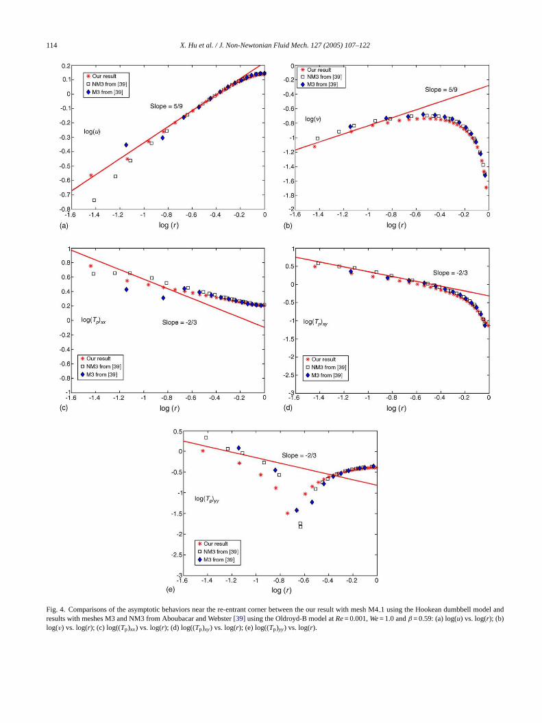
Fig. 4. Comparisons of the asymptotic behaviors near the re-entrant corner between the our result with mesh M41 using the Hookean dumbbell model andresults with meshes M3 and NM3 from Aboubacar and Webster[39] using the Oldroyd-B model atRe= 0.001,We= 1.0 andβ = 0.59: (a) log(u) vs. log(r); (b)log(v) vs. log(r); (c) log((Tp)xx) vs. log(r); (d) log((Tp)xy) vs. log(r); (e) log((Tp)yy) vs. log(r).


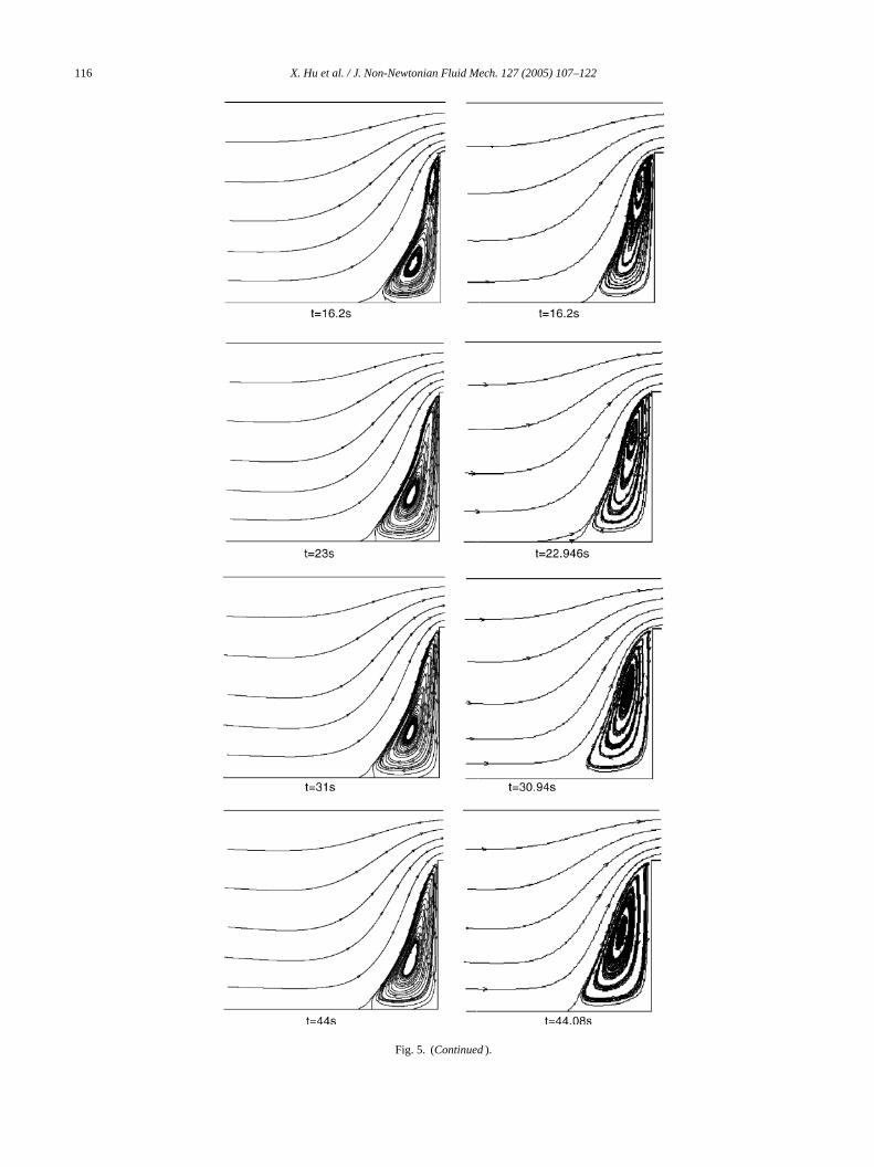
Fig. 5. Comparisons of the vortex evolution between our result with M41 (on the left) and that from Chung et al.[37] (on the right) atRe= 0.1,We= 9 andβ = 1/9.


Fig. 5. (Continued).


Fig. 6. Vortex evolution of the flow with the FENE dumbbell model atRe= 0.1,We= 9 andβ = 1/9.

In Table 1, we compare the mesh characteristics of thefollowing three meshes: M3 and NM3 from[39] and ourmesh M41 shown inFig. 2. Rmin is the minimum elementsize. In our study, we simply takeRmin = √

Smin, whereSminis the minimum element area.

In Fig. 3, we compare the stress patterns between our re-sult (on the left side) and their result with mesh NM3 (on theright side). There are some small differences between the tworesults, especially the zero-valued contour. But considering Fig. 7. Sketch of the upper half part geometry for the confined cylinder flow.


the errors from the stochastic processes of the CONNFFES-SIT approach, mesh density (especially the mesh densitynear the lower wall) and the order of our interpolation func-tion for stresses, it is fair to say that our result is reasonablygood.

Fig. 1also shows the geometry near the re-entrant corner.We set up a polar coordinate system by placing the originat the re-entrant corner. It was shown by Hinch[46] that thevelocity components would vanish asymptotically when ap-proaching the origin with the form ofr5/9, while the stresseswould be singular with the form ofr−2/3. Here,r is the mag-nitude of the radius vector pointing from the re-entrant cor-ner. We choose the velocities and stresses along the verticalline CO (θ =π/2) to compare our results with those fromAboubacar and Webster[39].

FromFig. 4(a–e), we see that our results and those from[39] based on the mesh grids M3 and NM3 are very closeand all agree with the analytical slope, as observed by theasymptotic behavior of the velocity components and stressesnear the re-entrant corner.

The next verification is to examine the evolutions andinteractions of the lip vortex and salient corner vortex. Weuse the same parameters (Re= 0.1, We= 9 andβ = 1/9) asAhn et al. [37]. Fig. 5 shows some differences betweenour result (on the left) and those from[37] (on the right)because they used a higher order time marching methoda t thes veryc texa ientc wille rgev

5be-

h r ther alentc m-p bellw theHβ ,W ni res ll att ellmt elsv

s isa ncesa arelsW

Fig. 8. Mesh grids Mesh3 and Mesh4 near the cylinder.

5.2. Confined cylinder flow (flow passing a cylinder in achannel)

This is also a classical benchmark case, which is a sim-plified form of the viscoelastic flow through the porous me-dia (usually the periodic boundary conditions are exerted atthe inlet and outlet). The results are useful for better un-derstanding mold filling in composite processing. Anotherusage can be found in the instrument technology for correct-ing the drag and heat transfer coefficient data when hot-wireprobes or sensors are placed in the non-Newtonian fluid flow-ing through a channel[9,41].

Table 2Mesh characteristic for confined cylinder flow

Meshes Elements orcontrol volumes

Nodes Rmin

Mesh3 5192 5395 0.015Mesh4 6632 6859 0.010M60 17400 – 0.00646M120 69600 – 0.00238M60(WR) – – 0.000613

F thMesh3 and Mesh4 and those from Alves et al.[44] and Fan et al.[45] withthe Oldroyd-B model atRe= 0.001,We= 0.7 andβ = 0.59.

nd a high-order element. Thus, the comparison aame time step may not be exact. Our results showlearly the evolutions and interactions of the lip vornd salient corner vortex. At first there is only the salorner vortex. When time increases, the lip vortexvolve and finally the two vortices merge into a single laortex.

.1.2. FENE dumbbell modelFor the FENE dumbbell model, the asymptotic

avior of the velocity components and stresses neae-entrant corner is also studied. Since there is no equivonstitutive equation for the FENE dumbbell, we coare our computational results from the FENE dumbith those of the Hookean dumbbell. We calculatedookean dumbbell model atRe= 0.001, We= 1.0 and= 1/9 and the FENE dumbbell model atRe= 0.001e= 1.0, β = 1/9 and b= 100 along the line CO show

n Fig. 1. All of the values for the FENE dumbbell alightly smaller than those for the Hookean dumbbehe same value of log(r). Since the Hookean dumbbodel can be achieved by settingb=∞, by increasing

he value ofb the differences between the two modanishes.

For the FENE dumbbell, the evolution of the vorticelmost the same as in the Hookean dumbbell. The differere that the sizes of the lip vortex and the final vortex

arger than those of the Hookean dumbbell. Results inFig. 6how the time evolutions for the FENE dumbbell atRe= 0.1,e= 9.0,β = 1/9 andb= 100.

ig. 9. Comparison of the stress component (Tp)xx between our results wi


Fig. 10. Comparisons of streamlines between the Newtonian fluid flow atRe= 0.001 and the flow with the Hookean dumbbell model atRe= 0.001,We= 0.7andβ = 0.59.

Many papers deal with this benchmark case using differentaspect ratios,Λ=R/H, whereR is the radius of the cylinderandH is the half distance between the two parallel plates.Here, we list some of them with the aspect ratio 1/2. Alves etal. [44] and Phan-Thien and Dou[47] used the finite volumemethod (FVM) to solve the confined cylinder flow with theUCM, Oldroyd-B and PTT fluid. Fan et al.[45] tested theMIX1/SUPG scheme in this benchmark case. Baaijens et al.[49] used the EVSS/DG method to calculate this flow with thePTT and Giesekus model. They also compared their modelwith experimental results. Hulsen et al.[7] and van Heel etal. [48] used the CONNFFESSIT approach to calculate thisflow with the Hookean, FENE, FENE-P and FENE-P∗ model.More literature can be found elsewhere[9].

Here, we are interested in the flow under non-zero Weis-senberg (We=λU/R, whereU is the average inlet velocityandR is the radius of the cylinder) and Reynolds numbers.The upper half geometry for this benchmark case is shownin Fig. 7. Both the upstream (from the inlet to the origin) andthe downstream lengths (from the origin to the outlet) are15. The gap of the channel is 4. Thus, the half height is 2.The radius of the cylinder is 1. The boundary conditions fordimensionless variables are given as follows:

(1) At the inlet AB, the velocity components are fixed. That2 t

heues

Fig. 11. Contours of the flow with the Hookean dumbbell model atRe= 0.001,We= 0.7 andβ = 0.59: (a)u contour, (b)v contour and (c) (Tp)xxcontour.

F 0 and the flow with the Hookean dumbbell model atRe= 10,We= 0.7 andβ = 0.59.

is, x component velocityu= 1.5(1− y /4), y componenvelocity v = 0; thus, the average inlet velocity is 1. TBrownian configuration vectors are fixed using valcalculated beforehand.

ig. 12. Comparisons of streamlines between Newtonian fluid flow atRe= 1


(2) On the walls CD and AF, the velocity conditions are theno-slip conditions,u = v = 0.

(3) At the outlet EF,σxx= 0,v = 0.(4) On the symmetric line BC and DE, we haveσxy= 0,v =

0.

The mesh characteristics for M60(WR), M120 and M60in [44] and our mesh grids of Mesh3 and Mesh4 shown inFig. 8 are listed inTable 2. Mesh4 is a wake-refined meshjust like the mesh M60(WR), while Mesh3 is more like themesh M120 or M60.

5.2.1. Hookean dumbbell modelFirst, we test our code by comparing the results at

Re= 0.001,We= 0.7 andβ = 0.59 with the Oldroyd-B fluidmodel[44,45]. Fig. 9shows one component of the polymerstresses (Tp)xx calculated from our mesh grids Mesh3 andMesh4 and M120 and M60(WR) from Alves et al.[44]. Theresult from Mesh4 is closer to the results from[44] in the wakethan that from Mesh3 because it has wake-refined mesh. Con-sidering the low mesh density in our calculations, our resultsappear very reasonable.

In Fig. 10, we compare the results with a Newtonianfluid atRe= 0.001 and with the Hookean dumbbell model atRe= 0.001,We= 0.7 andβ = 0.59 using the mesh grid Mesh4.It was found that the streamline for the Hookean dumbbelli ationp Ourr eta nt( yc -

FW

ilar results with the UCM and PTT model. The contour for(Tp)xx is similar to that from Owens et al.[50], although theyused different Deborah numbers.

We then increase the value of the Reynolds number andexamine the effect of the inertia term. Matallah et al.[38] andTownsend[43] carried out simulations on the flow passing acylinder in an infinite domain at high Reynolds number. Here,

Fig. 14. Comparisons of stress contours between two flows with the FENEdumbbell model at different Reynolds numbers: one is atRe= 0.001,We= 0.7andβ = 0.59 andb= 100 (on the top), the other is atRe= 10,We= 0.7,β = 0.59andb= 100 (on the bottom). (a) Contour comparison on (Tp)xx, (b) contourcomparison on (Tp)xy and (c) contour comparison on (Tp)yy.

s shifted upstream at a region close to the rear stagnoint, compared with the result for the Newtonian fluid.esults shown inFig. 10are similar to those given by Alvesl. [44]. The velocity componentsu, v and stress componeTp)xx contours are given inFig. 11(a–c). For the velocitomponent contours, Phan-Thien and Dou[47] showed sim

ig. 13. Contours of the flow with the Hookean dumbbell model atRe= 10,e= 0.7 andβ = 0.59: (a)u contour, (b)v contour and (c) (Tp)xx contour.


we study the differences between the Newtonian and non-Newtonian fluid flow using the same Reynolds number, buttwo different values of the Weissenberg number,We= 0.7 and1.0, for the Hookean dumbbell model. The Reynolds numberand the viscosity ratio are kept the same for the flow with theHookean dumbbell model, that is,Re= 10.0 andβ = 0.59.

When the Reynolds number is increased to 10, a second-order flow (vortex) behind the cylinder is observed as shownin Fig. 12. This second-order flow is shifted downstream be-hind the cylinder compared with the result for the Newtonianfluid [38,42,43].

When the Reynolds number is not zero, the convectioneffect propagates from upstream to downstream. The ve-locity patterns inFig. 13(a and b) shift further downstreamcompared withFig. 11(a and b). However, the stress patternaround the cylinder shifts upstream as shown inFig. 13(c).This occurs because as the Reynolds number increases, thevelocity gradient is larger at the front of the cylinder and thedumbbells stretch greatly there, giving higher stress values atthe front of the cylinder.

5.2.2. FENE dumbbell modelWe also compare the streamline patterns of the Newtonian

fluid flow atRe= 10 with those of the FENE dumbbell modelatRe= 10,We= 0.7 andβ = 0.59 andb= 100. The differencesare similar to those between the flow with Newtonian fluida thatt

hrees ENEdi theo chfi shiftu nationuh

6

thodu vis-c

e.g.,p us-i be-h heset onsb d-Bm

um-b ctioni Thise cantd

Acknowledgment

We are thankful to the Ohio Supercomputer Center forcomputation time.

References

[1] M. Laso, H.C.Ottinger, Calculation of viscoelastic flow using molec-ular models, J. Non-Newtonian Fluid Mech. 47 (1993) 1–20.

[2] K. Feigl, M. Laso, H.C.Ottinger, CONNFFESSIT approach for solv-ing a two-dimensional viscoelastic fluid problem, Macromolecules28 (1995) 3261–3274.

[3] M. Laso, M. Picasso, H.C.Ottinger, 2-D time-dependent viscoelasticflow calculations using CONNFFESSIT, AIChE J. 43 (4) (1997)877–892.

[4] C.C. Hua, J.D. Schieber, Viscoelastic flow through fibrous mediausing the CONNFFESSIT approach, J. Rheol. 42 (3) (1998) 477–491.

[5] M. Melchior, H.C.Ottinger, Variance reduced simulations of stochas-tic differential equations, J. Chem. Phys. 103 (21) (1995) 9506–9509.

[6] M. Melchior, H.C.Ottinger, Variance reduced simulations of polymerdynamics, J. Chem. Phys. 105 (8) (1996) 3316–3331.

[7] M.A. Hulsen, A.P.G. van Heel, B.H.A.A. van den Brule, Simulationof viscoelastic flows using Brownian configuration fields, J. Non-Newtonian Fluid Mech. 70 (1997) 79–101.

[8] H.C. Ottinger, B.H.A.A. van den Brule, M.A. Hulsen, Brownianconfiguration fields and variance reduced CONNFFESSIT, J. Non-Newtonian Fluid Mech. 70 (1997) 255–261.

ol-

[ ES-99)

[ sionnian

[ las-s, J.

[ sus-inter-

[ ticlepu-

[ tivecom-nian

[ La-on-

[ tionc ap-

[ s inoly-i. 51

[ ion99)

[ s of

nd the flow with the Hookean dumbbell model, excepthe differences are slightly smaller.

Fig. 14(a–c) compares the contour patterns of the ttress components between two results, both with the Fumbbell model atWe= 0.7,β = 0.59 andb= 100. One flow

s atRe= 0.001, which is shown on the top of each figure;ther flow is atRe= 10, which is shown on the bottom of eagure. Also, all the stress patterns around the cylinderpstream as the Reynolds number increases. The explased for the similar phenomenon in Section5.2.1) still holdsere.

. Conclusions

We have developed a modified DEVSS-G/SUPG mesing the CONNFFESSIT approach for handling theoelastic flow in complex geometry.

This method was applied to two benchmark cases,lanar 4:1 contraction flow and confined cylinder flow

ng the Hookean and FENE dumbbell models. The flowavior and vortex evolution were compared between t

wo dumbbell models and the Newtonian fluid. Comparisetween the Hookean dumbbell model and the Oldroyodel were satisfactory.The viscoelastic flow at the non-neglected Reynolds n

er was also examined. We found that the effect of conves important and changes the flow pattern significantly.ffect is important when the Reynolds number is signifiue to the very large characteristic velocity.

[9] R.G. Owens, T.N. Phillips, Computational Rheology, Imperial Clege Press, 2002.

10] J. Bonvin, M. Picasso, Variance reduction methods for CONNFFSIT like simulations, J. Non-Newtonian Fluid Mech. 84 (19191–215.

11] X.J. Fan, N. Phan-Thien, R. Zheng, Simulation of fiber suspenflows by the Brownian configuration field method, J. Non-NewtoFluid Mech. 84 (1999) 257–274.

12] M. Somasi, B. Khomami, Linear stability and dynamics of viscoetic flows using time-dependent stochastic simulation techniqueNon-Newtonian Fluid Mech. 93 (2000) 339–362.

13] N. Phan-Thien, X.J. Fan, R. Zheng, A numerical simulation ofpension flow using a constitutive model based on anisotropicparticle interactions, Rheol. Acta 39 (2000) 122–130.

14] P. Halin, G. Lielens, R. Keunings, V. Legat, The Lagrangian parmethod for macroscopic and micro–macro viscoelastic flow comtations, J. Non-Newtonian Fluid Mech. 79 (1998) 387–403.

15] X. Gallez, P. Halin, G. Lielens, R. Keunings, V. Legat, The adapLagrangian particle method for macroscopic and micro–macroputations of time-dependent viscoelastic flows, J. Non-NewtoFluid Mech. 80 (1999) 345–364.

16] P. Wapperom, R. Keunings, V. Legat, The backward-trackinggrangian particle method for transient viscoelastic flows, J. NNewtonian Fluid Mech. 91 (2000) 273–295.

17] Z. Ding, Numerical and experimental analysis on resin injecpultrusion (RIP) process—using macroscopic and microscopiproaches, Ph.D. Thesis, The Ohio State University, 2001.

18] C.C. Hua, J.D. Schieber, Application of kinetic theory modelspatiotemporal flows for polymer solutions, liquid crystals and pmer melts using the CONNFFESSIT approach, Chem. Eng. Sc(9) (1996) 1473–1485.

19] A.P.G. van Heel, M.A. Hulsen, B.H.A.A. van den Brule, Simulatof the Doi–Edwards model in complex flow, J. Rheol. 43 (5) (191239–1260.

20] R.B. Bird, C.F. Curtiss, R.C. Armstrong, O. Hassager, Dynamicpolymeric liquids, vol. 2, Wiley, New York, 1987.


[21] H.C. Ottinger, Stochastic Processes in Polymeric Fluids, Springer,Berlin, 1996.

[22] R.C. King, M.R. Apelian, R.C. Armstrong, R.A. Brown, Numeri-cally stable finite element techniques for viscoelastic calculations insmooth and singular geometries, J. Non-Newtonian Fluid Mech. 29(1988) 147–216.

[23] S.R. Burdette, P.J. Coates, R.C. Armstrong, R.A. Brown, Calcu-lations of viscoelastic flow through an axisymmetric corrugatedtube using the explicitly elliptic momentum equation formulation(EEME), J. Non-Newtonian Fluid Mech. 33 (1989) 1–23.

[24] D. Rajagopalan, R.C. Armstrong, R.A. Brown, Finite element meth-ods for calculation of steady viscoelastic flow using constitutiveequations with a Newtonian viscosity, J. Non-Newtonian Fluid Mech.36 (1990) 159–192.

[25] B. Khomami, K.K. Talwar, H.K. Ganpule, A comparative study ofhigher- and lower-order finite element techniques for computation ofviscoelastic flows, J. Rheol. 38 (2) (1994) 255–289.

[26] M.J. Szady, T.R. Salamon, A.W. Liu, D.E. Bornside, R.C. Arm-strong, R.A. Brown, A new mixed finite element for viscoelas-tic flows governed by differential constitutive equations, J. Non-Newtonian Fluid Mech. 59 (1995) 215–243.

[27] R. Guenette, M. Fortin, A new mixed finite element method for com-puting viscoelastic flows, J. Non-Newtonian Fluid Mech. 60 (1995)27–52.

[28] F.P.T. Baaijens, An iterative solver for the DEVSS/DG method withapplication to smooth and non-smooth flows of the upper convectedMaxwell fluid, J. Non-Newtonian Fluid Mech. 75 (1998) 119–138.

[29] A.C.B. Bogaerds, W.M.H. Verbeeten, G.W.M. Peters, F.P.T. Baaijens,3D viscoelastic analysis of a polymer solution in a complex flow,Comput. Methods Appl. Mech. Eng. 180 (1999) 413–430.

[30] A.W. Liu, D.E. Bornside, R.C. Armstrong, R.A. Brown, Viscoelasticers:on-

[ eardent99)

[ entvis-

thod:07.

[ in-n, J.

[ hod:99.

[35] M.A. Hulsen, Numerical simulation of the divergent flow regime ina circular contraction flow of a viscoelastic fluid, Theor. Comput.Fluid Dyn. 5 (1993) 33–48.

[36] Y. Fan, M.J. Crochet, High-order finite element methods forsteady viscoelastic flows, J. Non-Newtonian Fluid Mech. 57 (1995)283–311.

[37] K.H. Ahn, C.K. Chung, S.J. Song, S.J. Lee, Time Weissenberg Num-ber Superposition in a Vortex Growth Mechanism of a 4:1 PlanarContraction Flow, The 6th European Conference on Rheology, Ger-many, September 1–6, 2002.

[38] H. Matallah, P. Townsend, M.F. Webster, Recovery and stress-splitting schemes for viscoelastic flows, J. Non-Newtonian FluidMech. 75 (1998) 139–166.

[39] M. Aboubacar, M.F. Webster, A cell-vertex finite volume/elementmethod on triangles for abrupt contraction viscoelastic flows, J. Non-Newtonian Fluid Mech. 98 (2001) 83–106.

[40] S.J. Park, S.J. Lee, On the use of the open boundary conditionmethod in the numerical simulation of nonisothermal viscoelasticflow, J. Non-Newtonian Fluid Mech. 87 (1999) 197–214.

[41] D.F. James, A.J. Acosta, The laminar flow of dilute polymer so-lutions around circular cylinders, J. Fluid Mech. 42 (1970) 269–288.

[42] O. Manero, B. Mena, On the slow flow of viscoelastic liquids past acircular cylinder, J. Non-Newtonian Fluid Mech. 9 (1981) 379–387.

[43] P. Townsend, A numerical simulation of Newtonian and viscoelasticflow past stationary and rotating cylinders, J. Non-Newtonian FluidMech. 6 (1980) 219–243.

[44] M.A. Alves, F.T. Pinho, P.J. Oliverira, The flow of viscoelastic flu-ids past a cylinder: finite-volume high-resolution methods, J. Non-Newtonian Fluid Mech. 97 (2001) 207–232.

[45] Y. Fan, R.I. Tanner, N. Phan-Thien, Galerkin/least-square finite-nian

[ r, J.

[ co-266.

[ thenian

[ ters,low997)

[ ctralluid

flow of polymer solutions around a periodic, linear array of cylindcomparisons of predictions for microstructure and flow fields, J. NNewtonian Fluid Mech. 77 (1998) 153–190.

31] R. Sureshkumar, M.D. Smith, R.C. Armstrong, R.A. Brown, Linstability and dynamics of viscoelastic flows using time-depennumerical simulations, J. Non-Newtonian Fluid Mech. 82 (1957–104.

32] J. Sun, M.D. Smith, R.C. Armstrong, R.A. Brown, Finite elemmethod for viscoelastic flows based on the discrete adaptivecoelastic stress splitting and the discontinuous Galerkin meDAVSS-G/DG, J. Non-Newtonian Fluid Mech. 86 (1999) 281–3

33] T.J.R. Hughes, W.K. Liu, A. Brooks, Finite element analysis ofcompressible viscous flows by the penalty function formulatioComp. Phys. 30 (1979) 1–60.

34] J.C. Heinrich, D.W. Pepper, Intermediate Finite Element MetFluid Flow and Heat Transfer Applications, Taylor & Francis, 19

element methods for steady viscoelastic flows, J. Non-NewtoFluid Mech. 84 (1999) 233–256.

46] E.J. Hinch, The flow of an Oldroyd fluid around a sharp corneNon-Newtonian Fluid Mech. 50 (1993) 161–171.

47] N. Phan-Thien, H.-S. Dou, Viscoelastic flow past a cylinder: dragefficient, Comput. Methods Appl. Mech. Eng. 180 (1999) 243–

48] A.P.G. van Heel, M.A. Hulsen, B.H.A.A. van den Brule, Onselection of parameters in the FENE-P model, J. Non-NewtoFluid Mech. 75 (1998) 253–271.

49] F.P.T. Baaijens, S.H.A. Selen, H.P.W. Baaijens, G.W.M. PeH.E.H. Meijer, Viscoelastic flow past a confined cylinder of adensity polyethylene melt, J. Non-Newtonian Fluid Mech. 68 (1173–203.

50] R.G. Owens, C. Chauviere, T.N. Philips, A locally-upwinded spetechnique (LUST) for viscoelastic flows, J. Non-Newtonian FMech. 108 (2002) 49–71.

simulation of 2d transient viscoelastic flow using the connffessit approach

Documents