simulation environment for astrobee-rings system by
TRANSCRIPT

Simulation Environment for Astrobee-RINGS System
by
Tamerlan Yeleussizov
A thesis submitted to the college of engineering of
Florida Institute of Technology
in partial fulfillment of the requirements
for the degree of
Master
in
Mechanical Engineering
Melbourne, Florida
May, 2019

We the undersigned committee hereby approve the attached thesis, “Simulation
Environment for Astrobee-RINGS System” by Tamerlan Yeleussizov.
_________________________________________________
Hector Gutierrez, PhD
Professor
Mechanical and Civil Engineering
Major Advisor
_________________________________________________
Marius Silaghi, PhD
Associate Professor
Computer Engineering and Sciences
_________________________________________________
Beshoy Morkos, PhD
Associate Professor
Mechanical and Civil Engineering
_________________________________________________
Ashok Pand it, PhD
Professor and Head
Department of Mechanical and Civil Engineering

iii
Abstract
Title: Simulation Environment for Astrobee-RINGS System
Author: Tamerlan Yeleussizov
Advisor: Hector Gutierrez, Ph. D.
The thesis analyzes a flight software of a new free flying robot Astrobee, that will change
the current Synchronized Position Hold Engage Reorient Experimental Satellites
(SPHERES) on International Space Station (ISS). First, the main components of the flight
software were examined: Robotic Operating System (ROS), Gazebo and MATLAB.
During that phase, functionalities of ROS, Gazebo and MATLAB were analyzed, and it
was found how these components integrate between each other to build Astrobee flying
software.
Next, simulation of two Astrobees performing “in-home” and “torque” maneuvers was
executed. After a successful completion of simulation, results of Astrobee’s trajectory was
recorded. Then, by changing inertia matrix of Astrobees, Resonant Inductive Near-field
Generation System (RINGS) was added to the existing simulation. The same maneuvers
were performed, and the results were recorded. The last part of thesis developed a gazebo
model plugin that, according to the separation distance and angle of rotation of two
Astrobee-RINGS systems, calculated force and torque that must be applied to Astrobee-
RINGS system in the simulation. Then results of trajectory changes were recorded. They
were compared between original Astrobee and Astrobee-RINGS system, and between
gazebo force and torque plugin and Simulink force and torque plugin. It was concluded
that, Astrobee’s propulsion system is capable of moving Astrobee-RINGS system.
iv
Table of Contents
Table of Contents ................................................................................................... iv
List of Figures ........................................................................................................... v
Acknowledgement .................................................................................................. vi
Dedication .............................................................................................................. vii
Chapter 1 Background ............................................................................................ 1
Background: Astrobee .................................................................................................... 1 Background: RINGS ....................................................................................................... 2 Background: Flight Software and Simulation .............................................................. 4
Chapter 2 Simulation ............................................................................................... 8
Simulation: Description .................................................................................................. 8 Simulation: Changes to existing simulation .................................................................. 9 Simulation: Results ....................................................................................................... 10
Chapter 3 Discussion and Conclusion .................................................................. 14
Discussion ....................................................................................................................... 14 Conclusion ...................................................................................................................... 15
References ............................................................................................................... 16
Appendix A Installation and usage instructions for Astrobee flight software . 17
Appendix B Gazebo model plugin for electromagnetic force ............................ 21
Appendix C Gazebo model plugin for electromagnetic torque ......................... 23
Appendix D Code for plots generating ................................................................. 25
Appendix E Simulink diagram for force and torque model plugins ................. 27
v
List of Figures
Figure 1 — Rendering of Astrobee. ........................................................................... 2 Figure 2 — RINGS in tandem with SPHERES ......................................................... 3
Figure 3 — Gazebo window ...................................................................................... 5 Figure 4 — Simulink diagram of Astrobee's guidance, navigation and control ........ 6 Figure 5 — Interconnections of ROS nodes for Astrobee flight software ................. 6 Figure 6 — Simulation of Astrobee on ISS. .............................................................. 7
Figure 7 — 3-D model of Astrobee-RINGS system .................................................. 9 Figure 8 — Sample output of Gazebo model states. ................................................ 11
Figure 9 — X-positoin over time for original and changed inertia. ........................ 11 Figure 10 — Angle of rotation over time for original and changed inertia ............. 12
Figure 11 — X-position over time due to electromagnetic force ............................ 12
Figure 12 — Angle of rotation over time due to electromagnetic torque ................ 13
Figure 13 — X-position over time due to 1N force application .............................. 13

vi
Acknowledgement
I would first like to thank my thesis advisor Dr. Hector Gutierrez of the Mechanical and
Civil Engineering department at Florida Institute of Technology. The door to Dr. Gutierrez
office was always open whenever I ran into a trouble spot or had a question about my
research or writing. He consistently allowed this paper to be my own work but steered me
in the right the direction whenever he thought I needed it.
I must thank Astrobee flight software team at NASA Ames Research Center for their help
and guidance in my research.
I would also like to thank committee members who were involved in revision for this
research: Dr. Marius Silaghi and Dr. Beshoy Morkos. Without their participation and input,
revision could not have been successfully conducted.
Finally, I must express my very profound gratitude to my parents, my wife and to my
friends for providing me with unfailing support and continuous encouragement throughout
my years of study and through the process of researching and writing this thesis. This
accomplishment would not have been possible without them. Thank you.

vii
Dedication
I dedicate this to my mother and father.
1
Chapter 1
Background
Background: Astrobee
The Astrobee is a new free flying robot that has been in development phase since 2014 by
National Aeronautics and Space Administration (NASA). Astrobee will perform
Intravehicular Activity (IVA) on the International Space Station (ISS). Currently IVA free
flyers include: Synchronized Position Hold Engage and Reorient Experimental Satellites
(SPHERES), Int-Ball by Japan Aerospace Exploration Agency (JAXA), Crew Interactive
Mobile companioN (CIMON) by Airbus. The Astrobee will change the current SPHERES.
Astrobee is a cube shaped free flyer. The robot’s main purpose is to perform routine,
repetitive work for ISS crews, as well as help scientist in zero-g experiments. Some of the
Astrobee’s purpose will include conducting environment surveys, taking sensor readings,
and routine maintenance. Astrobee can autonomously navigate in US Orbital Segment
(USOS) using a fisheye sensor and a depth sensor. Also, an HD camera is present on
Astrobee to serve as a remotely controllable mobile camera platform. To benefit Human-
Robot Interaction (HRI) research the robot has touchscreen, multiple LED matrices,
microphones and speakers. On the other side of Astrobee, a detachable arm with gripper is
present to extend and hold to ISS handrails to minimize propulsion consumption. In the
future the robot can be used for research on satellite servicing. A picture of Astrobee is
shown on Figure 1. [1]
2
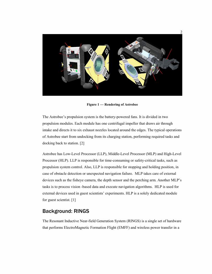
Figure 1 — Rendering of Astrobee
The Astrobee’s propulsion system is the battery-powered fans. It is divided in two
propulsion modules. Each module has one centrifugal impeller that draws air through
intake and directs it to six exhaust nozzles located around the edges. The typical operations
of Astrobee start from undocking from its charging station, performing required tasks and
docking back to station. [2]
Astrobee has Low-Level Processor (LLP), Middle-Level Processor (MLP) and High-Level
Processor (HLP). LLP is responsible for time-consuming or safety-critical tasks, such as
propulsion system control. Also, LLP is responsible for stopping and holding position, in
case of obstacle detection or unexpected navigation failure. MLP takes care of external
devices such as the fisheye camera, the depth sensor and the perching arm. Another MLP’s
tasks is to process vision -based data and execute navigation algorithms. HLP is used for
external devices used in guest scientists’ experiments. HLP is a solely dedicated module
for guest scientist. [1]
Background: RINGS
The Resonant Inductive Near-field Generation System (RINGS) is a single set of hardware
that performs ElectroMagnetic Formation Flight (EMFF) and wireless power transfer in a
3
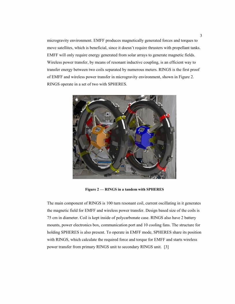
microgravity environment. EMFF produces magnetically generated forces and torques to
move satellites, which is beneficial, since it doesn’t require thrusters with propellant tanks.
EMFF will only require energy generated from solar arrays to generate magnetic fields.
Wireless power transfer, by means of resonant inductive coupling, is an efficient way to
transfer energy between two coils separated by numerous meters. RINGS is the first proof
of EMFF and wireless power transfer in microgravity environment, shown in Figure 2.
RINGS operate in a set of two with SPHERES.
Figure 2 — RINGS in a tandem with SPHERES
The main component of RINGS is 100 turn resonant coil, current oscillating in it generates
the magnetic field for EMFF and wireless power transfer. Design based size of the coils is
75 cm in diameter. Coil is kept inside of polycarbonate case. RINGS also have 2 battery
mounts, power electronics box, communication port and 10 cooling fans. The structure for
holding SPHERES is also present. To operate in EMFF mode, SPHERES share its position
with RINGS, which calculate the required force and torque for EMFF and starts wireless
power transfer from primary RINGS unit to secondary RINGS unit. [3]
4
Background: Flight Software and Simulation
The flight software for Astrobee consists of Robotic Operating System (ROS) and
MATLAB/Simulink. Gazebo is used as a robot simulation to demonstrate how the whole
system perform in real life.
The main purpose of ROS is to facilitate communication between ROS nodes. In other
words, it is a communication protocol for ROS nodes. Nodes are independent programs
that perform a given computation or task, meaning that they are software processes that can
register within ROS to communicate between each other. For example, one ROS node can
capture camera images, and then send it to another node for processing. The main
mechanism of ROS communication is done through passing and receiving messages. ROS
messages are defined by type of message and data format. Messages are organized into
topics. Each node can publish or subscribe to a topic. For example, one node can publish a
topic on system’s readiness to move, outputting message of a string type stating if system
is ready or not.[4]
Gazebo is a simulation environment, which mimics the robot behavior in real life. The
environment serves the following functions: Design of robot models, prototyping and
testing algorithms, simulation of sensors, cameras, forces and torques, 3-D object
utilization, modeling real-world dynamics. Gazebo makes use of SDF, which is XML
format describing robots and environments for robot simulators. In other words, it will
have description of kinematic, dynamics, as well as physical properties of an object in
simulation. An example of Gazebo window is shown in Figure 3. [4]

5
Figure 3 — Gazebo window
In the flight software MATLAB/Simulink code is responsible for guidance, navigation and
control. C++ code is auto-generated from Simulink forming one separate node of ROS.
The Simulink diagram is shown in Figure 4. Guidance, navigation and control consist of
following components: Extended Kalman filter for position estimation, control loop for
calculating desired forces and torques and force allocation module for translating control
loop commands to propulsion system.

6
Figure 4 —Simulink diagram of Astrobee’s guidance, navigation and control
Astrobee flight software performs a set of tasks, which include: Localization, motion
control and collision avoidance, autonomous docking and perching on handrails. Tasks are
done by having 46 ROS nodes, grouped into 14 processes, which communicate between
each other. The interconnections between nodes are shown in Figure 5.
Figure 5 — Interconnections of ROS nodes for Astrobee flight software
7
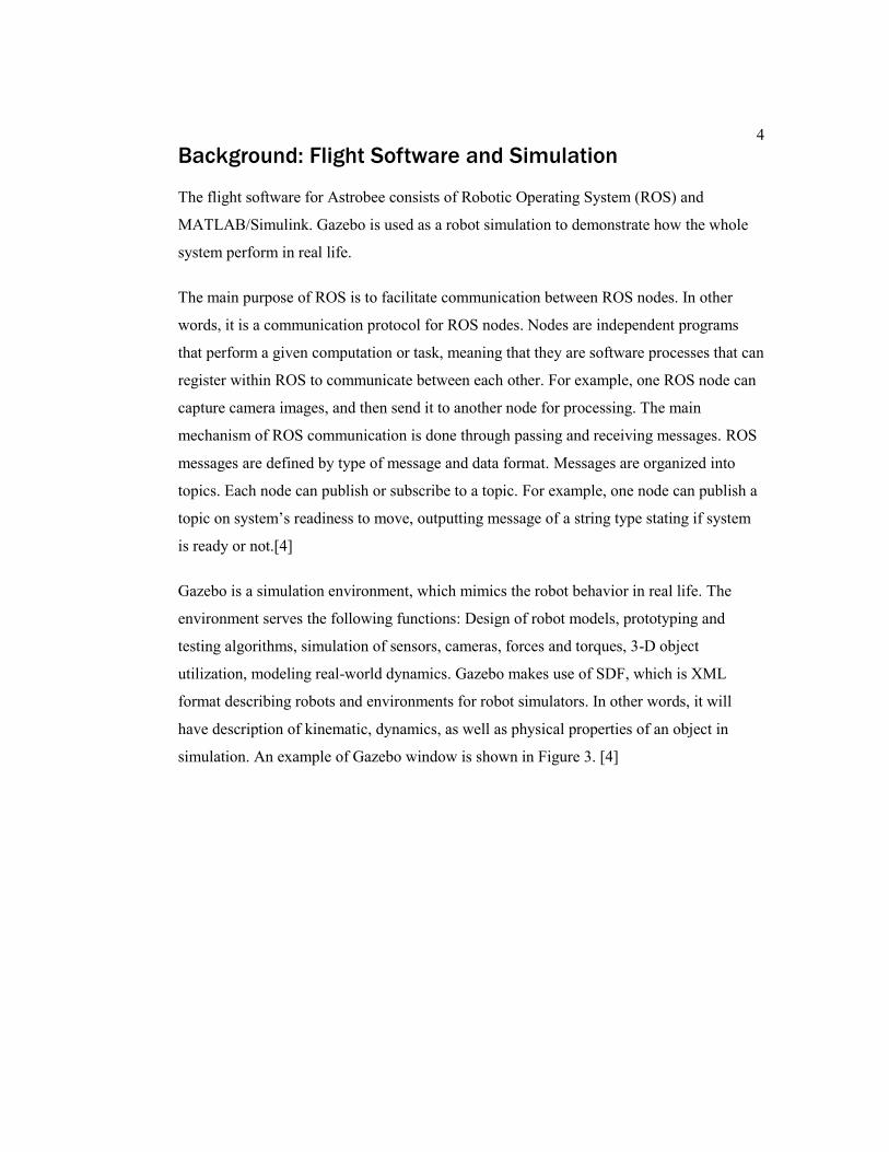
Since the software development is done virtually, before uploading it to actual prototype of
the robot, the simulator plays major role in the software. Gazebo is used to simulate the
Astrobee robot on ISS. The simulation allows to control the whole robot and get realistic
measurements for further analysis. Window of a single Astrobee is shown on Figure 6.[5]
Figure 6 —Simulation of Astrobee on ISS

8
Chapter 2
Simulation
Simulation: Description
The thesis work included three phases of simulation. The first was to start the Gazebo
simulation of ISS, spawn two Astrobees, and perform two maneuvers. The first maneuver
is “in home”. One of the Astrobees that was spawned was passive and held its position.
Another Astrobee was spawned at an axial separation distance of 1 meter, and it was
prompted to start the motion along the X axis to move closer to the passive Astrobee. The
second maneuver consisted of one Astrobee being passive and the other one performing
“torque maneuver”. The active Astrobee would rotate around Z axis to change its rotation
angle. After performing maneuver, trajectory along X axis of moving Astrobee and the
angle of rotation around of Z axis were recorded.
The mobility module of the Astrobee flight software is used to perform the above
maneuvers. The module allows users to move the designated Astrobee to a desired
position. Astrobees are distinguished by the namespace that was defined in the time of
spawning. The desired position was typed in the format X Y Z, where X Y Z are the
positions along the axes from the origin in meters. The desired angle of rotation was typed
in the format of W X Y Z, where W defines the angle of rotation in radians about the
X Y Z vector. Full instructions on software and simulation installations and operation of
the simulation are shown in Appendix A.
The second phase of the simulation consisted of changing inertia matrix, which implements
the addition of RINGS to simulation and performs same maneuvers as in phase one. In the
second phase the results of trajectory change were also recorded.
9
The third phase of simulation consisted of developing a Gazebo model plugin to simulate
the electromagnetic force and torque from RINGS and performing the same maneuvers as
in previous phases.
Simulation: Changes to existing simulation
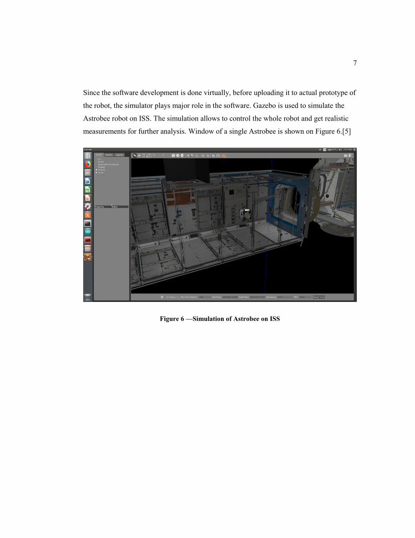
In order to execute the second phase of the simulation, the Astrobee’s inertia matrix was
changed from the original one. Changing the inertia matrix was completed to add RINGS
into the existing simulation. The Astrobee-RINGS system’s 3-D model is shown in
Figure 7.
Figure 7 —3-D model of Astrobee-RINGS system
The inertia matrix was changed in the SDF file that describes the Astrobee robot. The
original inertia matrix was as follows:

10
I=⟦0.187 0 0
0 0.187 00 0 0.187
⟧
It was changed to the following:
I=⟦0.999 0.045 0.1980.045 1.079 0.1290.198 0.129 0.711
⟧
Several equations were used to execute the third phase of simulation. First, for colinear and
coaxial translational motion, the following equation was used:
𝐹𝑥 =3𝜇0(𝑛𝐼𝜋𝑅𝑐
2)2
2𝜋𝑟4
Where 𝜇0 is magnetic permeability of free space, 4𝜋 × 10−7 𝐻/𝑚, n is a number of coil
turns, 𝑅𝑐 is the average radius of RINGS, 𝐼 is the current in coils, which is set to 13.7 A on
both coils, r is the axial distance between two coils.[6] For rotational motion, the following
formula was used:
𝑇𝑥 =𝜇0(𝑛𝐼𝜋𝑅𝑐
2)2
2𝑟4sin (𝛽)
Where 𝛽 is the angle of rotation around the Z axis. Two Gazebo model plugins were
developed according to equations for electromagnetic force and torque. The complete
codes can be found in Appendixes B and C. [7]
Simulation: Results
The results were recorded using the “echo” command for outputting the Gazebo model
states. Before outputting the results, a log file was started to record all the data. An
example of output is shown in Figure 8. After the data was processed in Excel by picking
desired data points, namely X position and angle of rotation around Z, of only active the
Astrobee-RINGS system. After all the data was recorded, MATLAB was used to plot
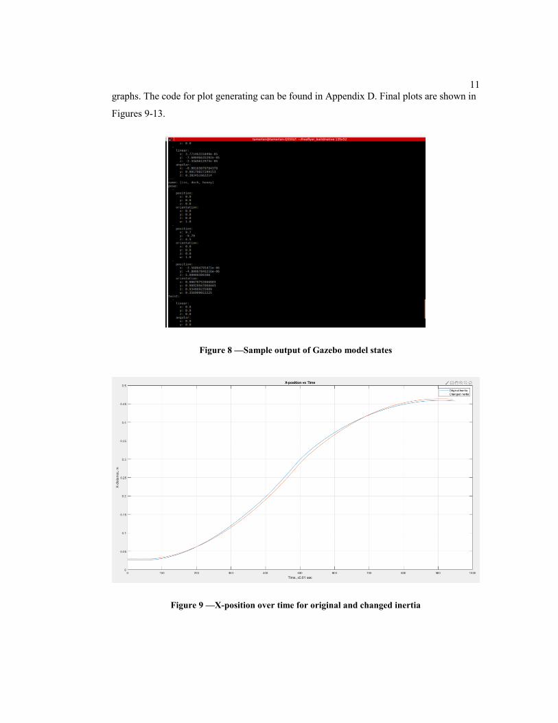
11
graphs. The code for plot generating can be found in Appendix D. Final plots are shown in
Figures 9-13.
Figure 8 —Sample output of Gazebo model states
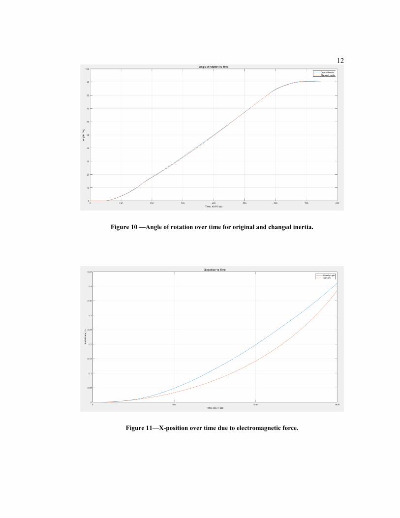
Figure 9 —X-position over time for original and changed inertia
12
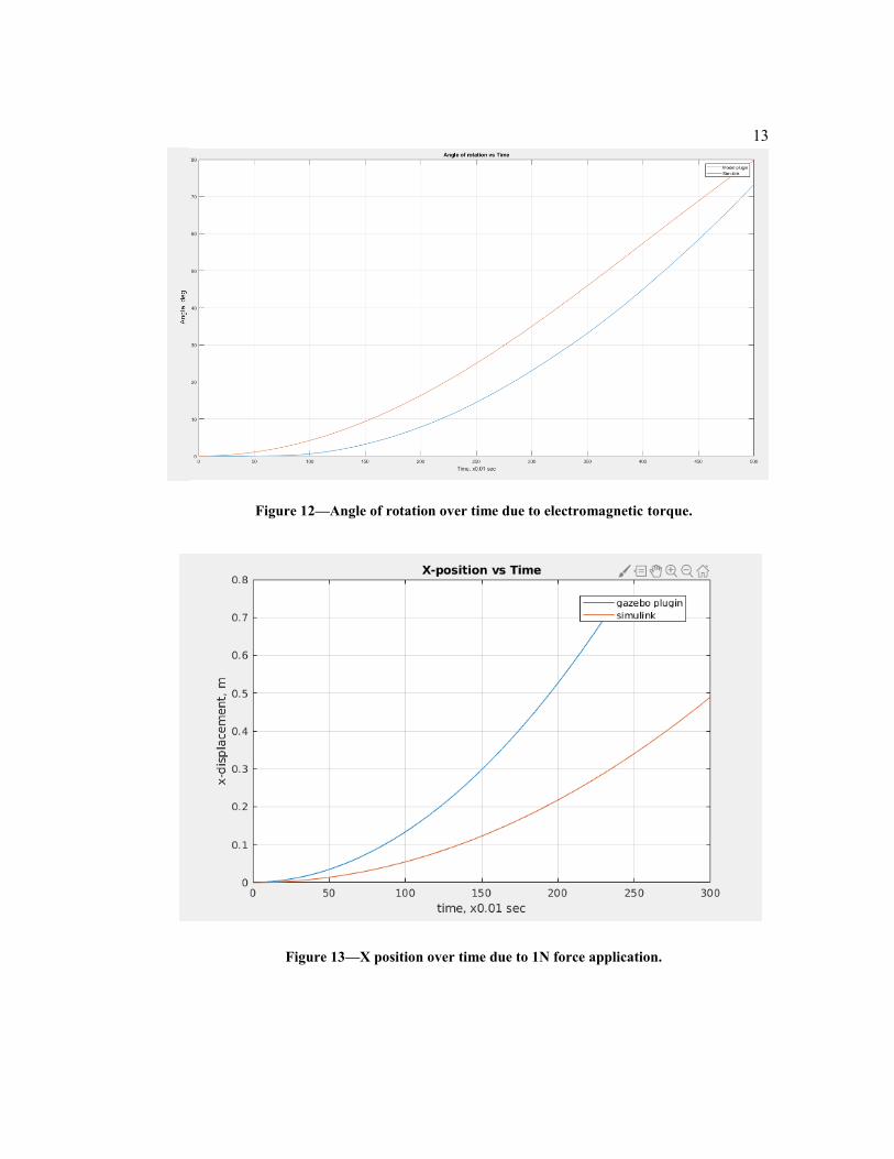
Figure 10 —Angle of rotation over time for original and changed inertia.
Figure 11—X-position over time due to electromagnetic force.
13
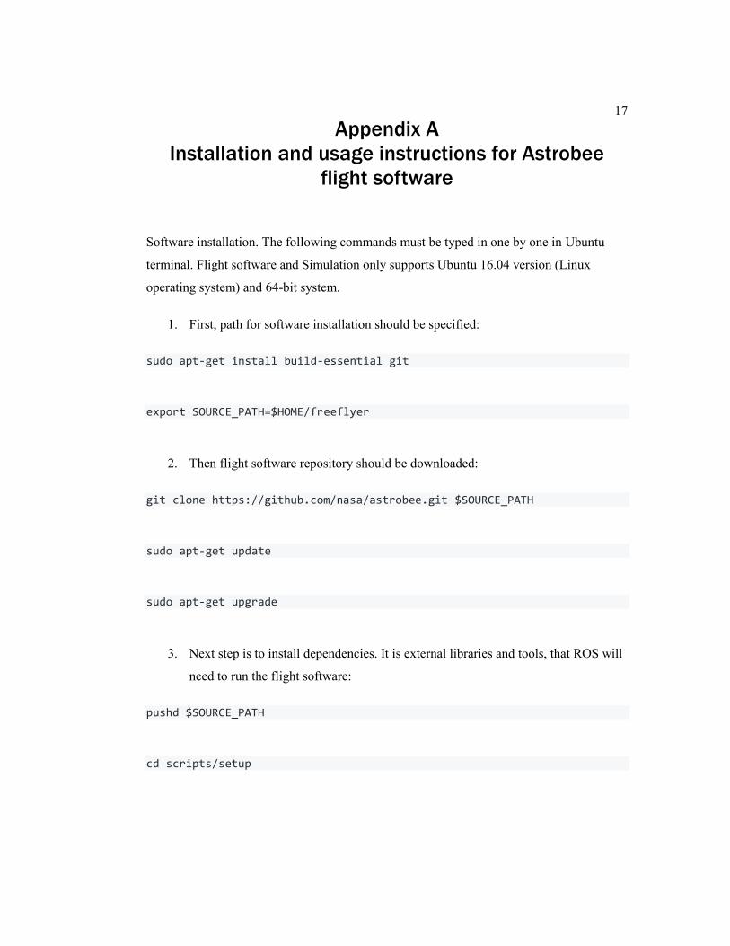
Figure 12—Angle of rotation over time due to electromagnetic torque.
Figure 13—X position over time due to 1N force application.

14
Chapter 3
Discussion and Conclusion
Discussion
The plot shown in Figure 9, represents the comparison between Astrobee and Astrobee-
RINGS system. Figure 9 shows X position of two systems over time. Two systems are
following the same trends. This is because the whole motion is carried by the Astrobee’s
propulsion system. Meaning that the Astrobee by itself can move Astrobee-RINGS system.
During the simulation Astrobee’s impeller speed was set at highest rate.
The plot shown in Figure 10, represents the same comparison between two systems.
However, in this case graphs represent the rotational angle around Z axis over time. Both
graphs have the same trend as previous X position plots. In this case, as in the previous
one, Astrobee’s propulsion system was responsible for the whole motion. One key
difference from the translational motion is that the rotational motion was carried out more
quickly. The translational and the rotational motion graphs show how Astrobee’s mobility
module commands to move slowly at the start, then speeds up and slows down by the
desired position.
The plot shown in Figure 11 represents the X position of Astrobee-RINGS system over
time. The motion was carried out by the Gazebo model plugin that applies electromagnetic
force to the system. The trajectory was compared to the X position changes due to
Newton’s second law. There were no other forces acting on the system, making Newton’s
second law a good benchmark. Simulink diagram was constructed to plot the X position as
a result of double integration of acceleration calculated from Newtons second law. The
diagram can be found in Appendix E. One of the difference form the Figure 9 is that the
total time of getting to the same position is greater in Figure 11. One of the reasons of such
results can be that for plotting Figure 11 Astrobee’s propulsion system was not used.
Propulsion system stayed in idle mode.

15
The plot shown in Figure 12 represents the angle of rotation around Z axis over time under
the application of the electromagnetic torque. The torque was applied by Gazebo model
plugin. The result was also compared to theoretical one as in Figure 11. However, for this
case torque equivalent of Newton’s second law was used. The Simulink diagram also can
be found in Appendix E. The graphs for the torques follow the same trends as the graphs
for the force. However, compared to Figure 10, it took shorter time getting to the same
position.
The graphs for Gazebo model plugin and Simulink models are not perfectly matching each
other. Another test was carried out to justify that trends are correct. Simple Gazebo model
plugin that applies 1N force in the X direction was compared to the Simulink model of 1N
force application. The result shown in Figure 13, both graphs are not matching as in
previous cases. The plot shows that there is discrepancy between the Gazebo model
plugins and the Simulink models. It possible that Astrobee’s air drag plugin, that was used
as a starting point for developing electromagnetic force and torque plugins, could have an
error. However, air drag plugin’s effect during normal Astrobee settings is almost
insignificant and might have been overlooked. The second reason of having discrepancy
can be the fact that Gazebo and Simulink are using different physics engine
Conclusion
To conclude, the Astrobee flight software has a complex architecture. However, it is still
possible to add changes to the software and to simulate the motion of the system.
Astrobee’s propulsion system is capable of moving Astrobee-RINGS system. However,
there are some limitations on the Gazebo model plugin, which can be the reason of creating
difference between the Gazebo model and the Simulink model, Another limitation is that
the MATLAB/Simulink are responsible for the guidance, navigation and control, which
cannot serve as a separate program. MATLAB/Simulink requires the full flight software in
order to operate. The Future work can include the development of the separate RINGS
model inside of Astorbee simulation environment. And adding other functionalities into the
simulation using plugins, as it was done in this thesis.

16
References
Jongwoon, Y., In-Won P., Vinh T., Jason Q. H. L., Trey S. (2015). Avionics and Perching
Systems of Free-Flying Robots for the International Space Station. 2015 IEEE
International Symposium.
Trey S., Jonathan B., Maria B., Terrence F., Christopher P., Hugo S., Ernest S. (2016).
Astrobee: A New Platform for Free-Flying Robotics on the International Space
Station. iSAIRAS.
Allison K.P., Dustin J.A., Raymond J. S., John M., Roedolph A. O., Alexander B., Gregory
E., Peter F., David W. M., Elisenda B. (2014). Demonstration of Electromagnetic
Formation Flight and Wireless Power Transfer. Journal of Spacecraft and Rockets,
Vol.51 (issue 6)
Thomas L. H., Carol F. (2016). ROS Robotics by Example.
Lorenzo F., Kathryn B., Brian C., Jesse F., Theodore M., Andrew S. (2018). Astrobee
Robot Software: Enabling Mobile Autonomy on the ISS.
Zeng G. and Hu M. (2012) Finite-time control for electromagnetic satellite formations.
Acta Astronautica, Vol.74.
Lafitte A. (2019) Electromagnetic Formation Flight with Resonant Inductive Near-Field
Generatoin System
17
Appendix A
Installation and usage instructions for Astrobee
flight software
Software installation. The following commands must be typed in one by one in Ubuntu
terminal. Flight software and Simulation only supports Ubuntu 16.04 version (Linux
operating system) and 64-bit system.
1. First, path for software installation should be specified:
sudo apt-get install build-essential git
export SOURCE_PATH=$HOME/freeflyer
2. Then flight software repository should be downloaded:
git clone https://github.com/nasa/astrobee.git $SOURCE_PATH
sudo apt-get update
sudo apt-get upgrade
3. Next step is to install dependencies. It is external libraries and tools, that ROS will
need to run the flight software:
pushd $SOURCE_PATH
cd scripts/setup

18
./add_ros_repository.sh
cd debians
./build_install_debians.sh
cd ../
./install_desktop_16_04_packages.sh
sudo rosdep init
rosdep update
popd
4. Next, preparing the build directory for compiling the code is required by running
configure script:
export BUILD_PATH=$HOME/freeflyer_build/native
export INSTALL_PATH=$HOME/freeflyer_install/native
pushd $SOURCE_PATH
./scripts/configure.sh -l -F -D

19
popd
5. Building the code. It is important step, since at this step codes are compiled. If any
changes made to the software, these commands should be run again.
cd freeflyer_build
cd native
make -j2
popd
6. Setting up environment. This step should be noted, since environment set up
should occur every time computer turns on.
cd freeflyer_build
cd native
source devel/setup.bash
7. Usage instructions. Only after the environment set up, following commands can
run. The software should be used by following: having several terminals open is
required, since once terminal is running a process, it can not run second one at the
same window.
Termianl A: Starts a simulation of ISS in Gazebo

20
roslaunch astrobee sim.launch dds:=false sviz:=true
Terminal B: Spawns an Astrobee robot to running ISS simulation under the namespace
Honey (now all the commands dedicated to Honey, should be differentiated by “-ns
honey”) at the position of X=0 m Y=0 m Z=5 m
roslaunch astrobee spawn.launch ns:=honey pose:="0 0 0"
Terminal C: Spawns an Astrobee robot to running ISS simulation under the namespace
Bumble at the position X=5 m Y=0 m Z=5m
roslaunch astrobee spawn.launch ns:=bumble pose:="5 0 5"
Terminal D: Moves the Honey Astrobee to a new position X=3 m Y=0 m Z=5 m
rosrun mobility teleop -ns honey -move -pos "3 0 5"
Terminal E: Rotates the Bumble Astrobee around Z-axis to 90 degrees. Note, there are
four entries, W=1.5 (angle of rotation in radians) X=0 Y=0 Z=1 (vector around which the
robot will rotate).
rosrun mobility teleop -move -att "-1.5 0 0 1"
Terminal F: Creates log file and outputs all existing in simulation model states
script log.txt rostopic echo gazebo/model_states exit

21
Appendix B
Gazebo model plugin for electromagnetic force
#include <ros/ros.h>
// Gazebo includes
#include <astrobee_gazebo/astrobee_gazebo.h>
#include <math.h>
namespace gazebo {
// This class is a plugin that calls the GNC autocode to predict
// the forced to be applied to the rigid body
class GazeboModelPluginEMForce : public FreeFlyerModelPlugin {
public:
GazeboModelPluginEMForce() : FreeFlyerModelPlugin("gazebo_emforce", "")
~GazeboModelPluginEMForce() {
event::Events::DisconnectWorldUpdateBegin(update_);
}
protected:
// Called when the plugin is loaded into the simulator
void LoadCallback(
ros::NodeHandle *nh, physics::ModelPtr model, sdf::ElementPtr sdf) {
// Called before each iteration of simulated world update
next_tick_ = GetWorld()->GetSimTime();
update_ = event::Events::ConnectWorldUpdateBegin(
std::bind(&GazeboModelPluginEMForce::WorldUpdateCallback, this));
}
// Called on simulation reset
void Reset() {
next_tick_ = GetWorld()->GetSimTime();
}

22
// Called on each sensor update event
void WorldUpdateCallback() {
// Calculate EMforce
double x;
gazebo::math::Pose pose;
pose = this->GetModel()->GetWorldPose();
math::Vector3 v(0, 0, 0);
v = pose.pos;
x=v.x;
//Calculating force
double f;
f=(3*0.00000047*100*100*13.7*13.7*3.14*pow(4,0.35))/(2*3.14*pow(4,(abs(1-
x))));
math::Vector3 emforce(f,0,0);
// Apply the force to the model
GetLink()->AddForce(emforce_);
}
private:
common::Time next_tick_;
event::ConnectionPtr update_;
};
// Register this plugin with the simulator
GZ_REGISTER_MODEL_PLUGIN(GazeboModelPluginEMForce)
} // namespace gazebo

23
Appendix C
Gazebo model plugin for electromagnetic torque
#include <ros/ros.h>
// Gazebo includes
#include <astrobee_gazebo/astrobee_gazebo.h>
#include <math.h>
namespace gazebo {
// This class is a plugin that calls the GNC autocode to predict
// the forced to be applied to the rigid body
class GazeboModelPluginEMTorque : public FreeFlyerModelPlugin {
public:
GazeboModelPluginEMTorque() : FreeFlyerModelPlugin("gazebo_emforce", "")
~GazeboModelPluginEMTorque() {
event::Events::DisconnectWorldUpdateBegin(update_);
}
protected:
// Called when the plugin is loaded into the simulator
void LoadCallback(
ros::NodeHandle *nh, physics::ModelPtr model, sdf::ElementPtr sdf) {
// Called before each iteration of simulated world update
next_tick_ = GetWorld()->GetSimTime();
update_ = event::Events::ConnectWorldUpdateBegin(
std::bind(&GazeboModelPluginEMTorque::WorldUpdateCallback, this));
}
// Called on simulation reset
void Reset() {
next_tick_ = GetWorld()->GetSimTime();

24
}
// Called on each sensor update event
void WorldUpdateCallback() {
// Calculate EMTorque
double x;
gazebo::math::Pose pose;
pose = this->GetModel()->GetWorldPose();
math::Vector3 v(0, 0, 0);
v = pose.rot;
x = v.w;
double angle,a;
angle=2*asin(x));
a=angle*(180/3.14);
double t;
t_ =
(0.00000047*100*100*13.7*13.7*3.14*0.35*0.35*0.35*0.35*sin(a))/(2*pow(3,1))
;// Calculating torque
// Apply the torque to the model
math::Vector3 emtorque(t,0,0);
GetLink()->AddTorque(emtorque);
}
private:
common::Time next_tick_;
event::ConnectionPtr update_;
};
// Register this plugin with the simulator
GZ_REGISTER_MODEL_PLUGIN(GazeboModelPluginEMTorque)
} // namespace gazebo

25
Appendix D
Code for plots generating
clc; t1=0:951; t2=0:733; t3=0:943; t4=0:746; t5=0:1500; t6=0:500; P1M2=2*acosd(P1M2r); P2M2=2*acosd(P2M2r); P3M2=2*acosd(P3M2r); figure (1) plot (t1,P1M1); hold on; grid on; plot (t3,P2M1); title 'X-position vs Time'; legend('Original inertia', 'Changed inertia') xlabel ('Time, x0.01 sec'); ylabel ('X-distance, m') figure (2) plot (t2,P1M2); hold on; grid on; plot (t4,P2M2); title 'Angle of rotation vs Time'; legend('Original inertia', 'Changed inertia') xlabel ('Time, x0.01 sec'); ylabel ('Angle, deg') figure (3) plot (t5,P3M1);
26
hold on; title 'X-position vs Time'; plot (t5,NLdistance1); legend('Model plugin', 'Simulink') xlabel ('Time, x0.01 sec'); ylabel ('X-distance, m') grid on; figure (4) plot (t6,P3M2); hold on; title 'Angle of rotation vs Time'; plot (t6,NLangle1); legend('Model plugin', 'Simulink') xlabel ('Time, x0.01 sec'); ylabel ('Angle, m') grid on;
27
Appendix E
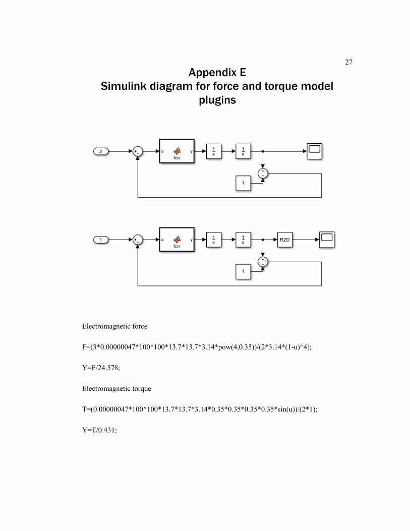
Simulink diagram for force and torque model
plugins
Electromagnetic force
F=(3*0.00000047*100*100*13.7*13.7*3.14*pow(4,0.35))/(2*3.14*(1-u)^4);
Y=F/24.578;
Electromagnetic torque
T=(0.00000047*100*100*13.7*13.7*3.14*0.35*0.35*0.35*0.35*sin(u))/(2*1);
Y=T/0.431;