simulation basics - university of...

Module 8, Slide 1 ECE/CS 541: Computer System Analysis. ©2005 William H. Sanders. All rights reserved. Do not copy or distribute to others without the permission of the author.

Simulation Basics


Motivation

•  High-level formalisms (like SANs) make it easy to specify realistic systems, but they also make it easy to specify systems that have unreasonably large state spaces.

•  State-of-the-art tools (like Mobius) can handle state-level models with a few ten’s of million states, but not more.

•  When state spaces become too large, discrete event simulation is often a viable alternative.

•  Discrete-event simulation can be used to solve models with arbitrarily large state spaces, as long as the desired measure is not based on a “rare event.”

•  When “rare events” are present, variance reduction techniques can sometimes be used.


Simulation as Model Experimentation •  State-based methods (such as Markov chains) work by enumerating all possible

states a system can be in, and then invoking a numerical solution method on the generated state space.

•  Simulation, on the other hand, generates one or more trajectories (possible behaviors from the high-level model), and collects statistics from these trajectories to estimate the desired performance/dependability measures.

•  Just how this trajectory is generated depends on the: –  nature of the notion of state (continuous or discrete) –  type of stochastic process (e.g., ergodic, reducible) –  nature of the measure desired (transient or steady-state) –  types of delay distributions considered (exponential or general)

•  We will consider each of these issues in this module, as well as the simulation of systems with rare events.


Types of Simulation Continuous-state simulation is applicable to systems where the notion of state is continuous and typically involves solving (numerically) systems of differential equations. Circuit-level simulators are an example of continuous-state simulation.

Discrete-event simulation is applicable to systems in which the state of the system changes at discrete instants of time, with a finite number of changes occurring in any finite interval of time.

Since we will focus on validating end-to-end systems, rather than circuits, we will focus on discrete-event simulation.

There are two types of discrete-event simulation execution algorithms: –  Fixed-time-stamp advance –  Variable-time-stamp advance


Fixed-Time-Stamp Advance Simulation •  Simulation clock is incremented a fixed time Δt at each step of the simulation. •  After each time increment, each event type (e.g., activity in a SAN) is checked

to see if it should have completed during the time of the last increment. •  All event types that should have completed are completed and a new state of the

model is generated. •  Rules must be given to determine the ordering of events that occur in each

interval of time. •  Example:

•  Good for all models where most events happen at fixed increments of time (e.g., gate-level simulations).

•  Has the advantage that no “future event list” needs to be maintained. •  Can be inefficient if events occur in a bursty manner, relative to time-step used.

2Δt Δt 3Δt 4Δt 5Δt 0 e1 e2 e5

e4 e3 e6


Variable-Time Step Advance Simulation

•  Simulation clock advanced a variable amount of time each step of the simulation, to time of next event.

•  If all event times are exponentially distributed, the next event to complete and time of next event can be determined using the equation for the minimum of n exponentials (since memoryless), and no “future event list” is needed.

•  If event times are general (have memory) then “future event list” is needed. •  Has the advantage (over fixed-time-stamp increment) that periods of inactivity

are skipped over, and models with a bursty occurrence of events are not inefficient.


Basic Variable-Time-Step Advance Simulation Loop for SANs

A) Set list_of_active_activities to null. B) Set current_marking to initial_marking. C) Generate potential_completion_time for each activity that may complete in the

current_marking and add to list_of_active_activities. D) While list_of_active_activities ≠ null:

1) Set current_activity to activity with earliest potential_completion_time. 2) Remove current_activity from list_of_active_activities. 3) Compute new_marking by selecting a case of current_activity, and executing

appropriate input and output gates. 4) Remove all activities from list_of_active_activities that are not enabled in

new_marking. 5) Remove all activities from list_of_active_activities for which new_marking is a

reactivation marking. 6) Select a potential_completion_time for all activities that are enabled in

new_marking but not on list_of_active_activities and add them to list_of_active_activities.

E) End While.


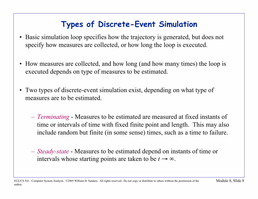
Types of Discrete-Event Simulation •  Basic simulation loop specifies how the trajectory is generated, but does not

specify how measures are collected, or how long the loop is executed.

•  How measures are collected, and how long (and how many times) the loop is executed depends on type of measures to be estimated.

•  Two types of discrete-event simulation exist, depending on what type of measures are to be estimated.

–  Terminating - Measures to be estimated are measured at fixed instants of time or intervals of time with fixed finite point and length. This may also include random but finite (in some sense) times, such as a time to failure.

–  Steady-state - Measures to be estimated depend on instants of time or intervals whose starting points are taken to be t → ∞.


Issues in Discrete-Event Simulation 1) How to generate potential completion times for events

2) How to estimate dependability measures from generated trajectories –  Transient measures –  Steady-state measures

3) How to implement the basic simulation loop –  Sequential or parallel


Generation of Potential Completion Times 1) Generation of uniform [0,1] random variates

–  Used as a basis for all random variate samples –  Types

•  Linear congruential generators •  Tausworthe generators •  Other types of generators

–  Tests of uniform [0,1] generators

2) Generation of non-uniform random variates –  Inverse transform technique –  Convolution technique –  Composition technique –  Acceptance-rejection technique –  Technique for discrete random variates

3) Recommendations/Issues


Generation of Uniform [0,1] Random Number Samples Goal: Generate sequence of numbers that appears to have come from uniform [0,1]

random variable.

Importance: Can be used as a basis for all random variates.

Issues: 1) Goal isn’t to be random (non-reproducible), but to appear to be random. 2) Many methods to do this (historically), many of them bad (picking

numbers out of phone books, computing π to a million digits, counting gamma rays, etc.).

3) Generator should be fast, and not need much storage. 4) Should be reproducible (hence the appearance of randomness, not the

reality). 5) Should be able to generate multiple sequences or streams of random

numbers.


Linear Congruential Generators (LCGs) •  Introduced by D. H. Lehmer (1951). He obtained

xn = an mod m xn = (axn - 1) mod m

•  Today, LCGs take the following form:

xn = (axn - 1 + b) mod m, where

xn are integers between 0 and m - 1 a, b, m non-negative integers

•  If a, b, m chosen correctly, sequence of numbers can appear to be uniform and have large period (up to m).

•  LCGs can be implemented efficiently, using only integer arithmetic.

•  LCGs have been studied extensively; good choices of a, b, and m are known. See, e.g., Law and Kelton (1991), Jain (1991).


Tausworthe Generators

•  Proposed by Tausworthe (1965), and are related to cryptographic methods.

•  Operate on a sequence of binary digits (0,1). Numbers are formed by selecting bits from the generated sequence to form an integer or fraction.

•  A Tausworthe generator has the following form: bn = cq - 1bn - 1 ⊕ cq - 2bn - 2 ⊕ . . . ⊕ c0bn - q where bn is the nth bit, and ci (i = 0 to q - 1) are binary coefficients.

•  As with LCGs, analysis has been done to determine good choices of the ci.

•  Less popular than LCGs, but fairly well accepted.


Generation of Non-Uniform Random Variates •  Suppose you have a uniform [0,1] random variable, and you wish to have a

random variable X with CDF FX. How do we do this?

•  All other random variates can be generated from uniform [0,1] random variates.

•  Methods to generate non-uniform random variates include: –  Inverse Transform - Direct computation from single uniform [0,1] variable

based on observation about distribution. –  Convolution - Used for random variables that can be expressed as sum of

other random variables. –  Composition - Used when the distribution of the desired random variable

can be expressed as a weighted sum of the distributions of other random variables.

–  Acceptance-Rejection - Uses multiple uniform [0,1] variables and a function that “majorizes” the density of the random variate to be generated.


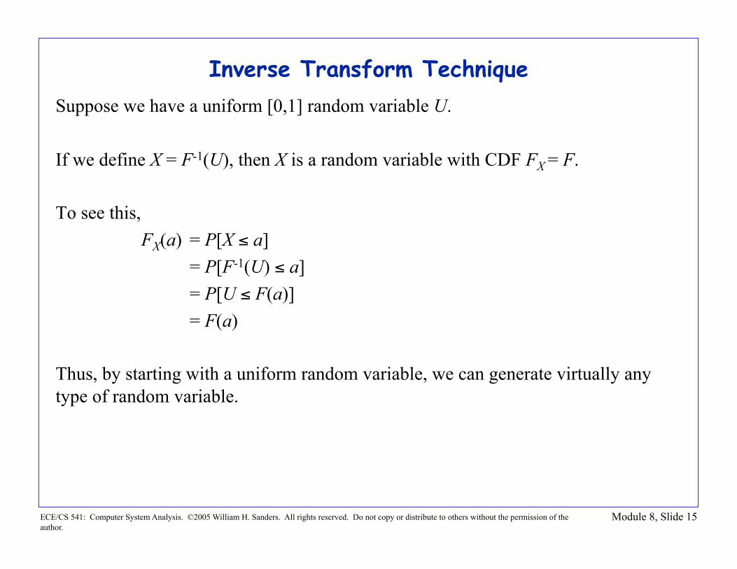
Inverse Transform Technique Suppose we have a uniform [0,1] random variable U.

If we define X = F-1(U), then X is a random variable with CDF FX = F.

To see this, FX(a) = P[X ≤ a] = P[F-1(U) ≤ a] = P[U ≤ F(a)] = F(a)

Thus, by starting with a uniform random variable, we can generate virtually any type of random variable.


Inverse Transform Technique : Examples Technique is to set up equation F(x) = U, and solve for x

Exponential

Uniform [a,b]


Inverse Transform Technique : Examples Weibull


Convolution Technique •  Technique can be used for all random variables X that can be expressed as the

sum of n random variables X = Y1 + Y2 + Y3 + . . . + Yn

•  In this case, one can generate a random variate X by generating n random variates, one from each of the Yi, and summing them.

•  Examples of random variables: –  Sum of n Bernoulli random variables is a binomial random variable. –  Sum of n exponential random variables is an n-Erlang random variable.


Composition Technique •  Technique can be used when the distribution of a desired random variable can

be expressed as a weighted sum of other distributions.

•  In this case F(x) can be expressed as

•  The composition technique is as follows: 1) Generate random variate i such that P[I = i] = pi for i = 0, 1, . . . (This can be done as discussed for discrete random variables.) 2) Return x as random variate from distribution Fi(x), where i is as chosen

above.

•  A variant of composition can also be used if the density function of the desired random variable can be expressed as weighted sum of other density functions.

( ) ( )

∑

∑∞

=

∞

=

=≥

=

0

0

.1 ,0 where

iii

iii

pp

xFpxF


Acceptance-Rejection Technique •  Indirect method for generating random variates that should be used when other

methods fail or are inefficient. •  Must find a function m(x) that “majorizes” the density function f(x) of the

desired distribution. m(x) majorizes f(x) if m(x) ≥ f(x) for all x. •  Note:

•  If random variates for m(x) can be easily computed, then random variates for f(x) can be found as follows: 1) Generate y with density m′(x) 2) Generate u with uniform [0,1] distribution

3)

( ) ( ) ( )

( ) function.density a is )(but

function,density ay necessarilnot is so ,1

cxmxm

xmdxxfdxxmc

=′

=≥= ∫∫∞

∞−

∞

∞−

1. goto else ,return ,)()( If yymyfu ≤


Generating Non-homogeneous Poisson Process •  A NHPP has independent increments and time-dependent rate

–  Means that probability of one event in (t-h/2,t+h/2) is

•  Suppose there exists with for all t •  Sample a homogeneous Poisson process with rate

–  event occurs at time t, accept with probability


Generating Discrete Random Variates

•  Useful for generating any discrete distribution, e.g., case probabilities in a SAN. •  More efficient algorithms exist for special cases; we will review most general

case. •  Suppose random variable has probability distribution p(0), p(1), p(2), . . . on

non-negative integers. Then a random variate for this random variable can be generated using the inverse transform method:

1) Generate u with distribution uniform [0,1] 2) Return j satisfying

( ) ( )∑∑=

−

=

<≤j

i

j

iipuip

0

1

0

Module 8, Slide 23

Generating Discrete Random Variables using Alias Table

•  Create an “alias” table with N entries. Entry i has the form •  To sample,

–  Choose entry i with probability 1/N (i.e., uniformly sample table entry) –  –  The magic part is building the table to work right

•  Notice that original values with probability greater than 1/N appear more than once in the alias table

•  Making the alias table –  Sort values into sets G (those with probability < 1/N) and H (all others) –  Initialize each with “residual probability” equal to original probability

ECE/CS 541: Computer System Analysis. ©2005 William H. Sanders. All rights reserved. Do not copy or distribute to others without the permission of the author.

Module 8, Slide 24

Generating Discrete Random Variables using Alias Table

•  Making the alias table –  Sort values into sets G (those with probability < 1/N) and H (all others) –  Initialize each with “residual probability” r equal to original probability p –  For i=1 to N

•  Choose some in G –  Set –  Make first component –  Choose , make 2nd component –  Set –  Reclassify to be in H or G

ECE/CS 541: Computer System Analysis. ©2005 William H. Sanders. All rights reserved. Do not copy or distribute to others without the permission of the author.


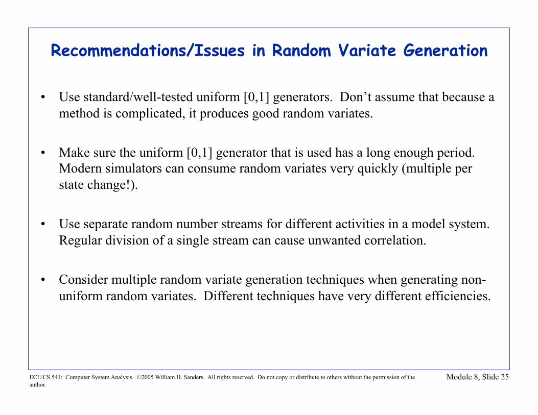
Recommendations/Issues in Random Variate Generation

•  Use standard/well-tested uniform [0,1] generators. Don’t assume that because a method is complicated, it produces good random variates.

•  Make sure the uniform [0,1] generator that is used has a long enough period. Modern simulators can consume random variates very quickly (multiple per state change!).

•  Use separate random number streams for different activities in a model system. Regular division of a single stream can cause unwanted correlation.

•  Consider multiple random variate generation techniques when generating non-uniform random variates. Different techniques have very different efficiencies.


Estimating Dependability Measures: Estimators and Confidence Intervals

•  An execution of the basic simulation loop produces a single trajectory (one possible behavior of the system).

•  Common mistake is to run the basic simulation loop a single time, and presume observations generated are “the answer.”

•  Many trajectories and/or observations are needed to understand a system’s behavior.

•  Need concept of estimators and confidence intervals from statistics: –  Estimators provide an estimate of some characteristic (e.g., mean or

variance) of the measure. –  Confidence intervals provide an estimate of how “accurate” an estimator is.


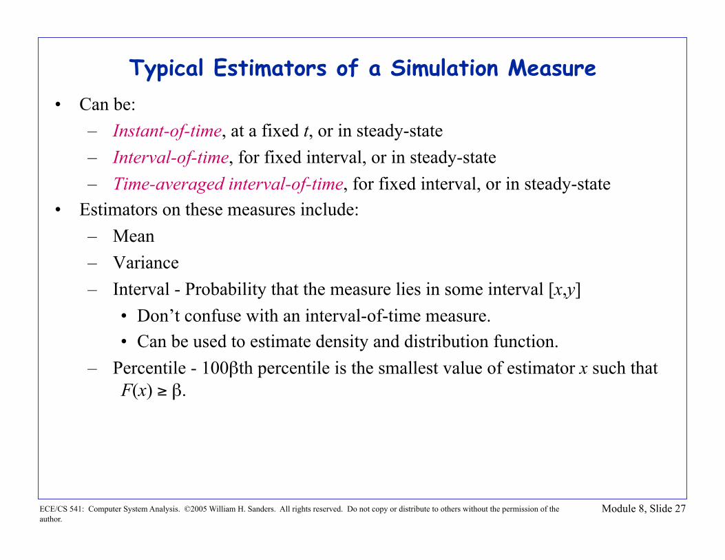
Typical Estimators of a Simulation Measure •  Can be:

–  Instant-of-time, at a fixed t, or in steady-state –  Interval-of-time, for fixed interval, or in steady-state –  Time-averaged interval-of-time, for fixed interval, or in steady-state

•  Estimators on these measures include: –  Mean –  Variance –  Interval - Probability that the measure lies in some interval [x,y]

•  Don’t confuse with an interval-of-time measure. •  Can be used to estimate density and distribution function.

–  Percentile - 100βth percentile is the smallest value of estimator x such that F(x) ≥ β.


Different Types of Processes and Measures Require Different Statistical Techniques

•  Transient measures (terminating simulation): –  Multiple trajectories are generated by running basic simulation loop multiple

times using different random number streams. Called Independent Replications.

–  Each trajectory used to generate one observation of each measure. •  Steady-State measures (steady-state simulation):

–  Initial transient must be discarded before observations are collected. –  If the system is ergodic (irreducible, recurrent non-null, aperiodic), a single

long trajectory can be used to generate multiple observations of each measure.

–  For all other systems, multiple trajectories are needed.


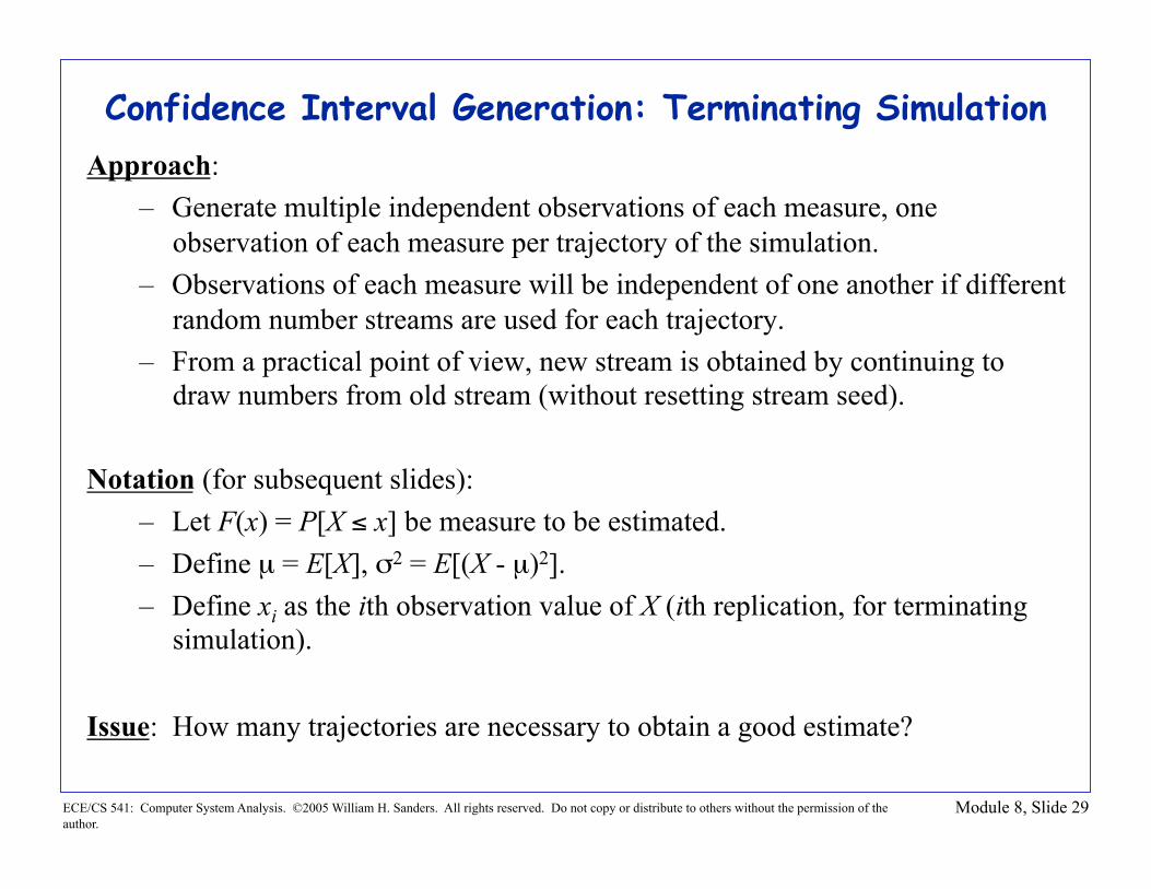
Confidence Interval Generation: Terminating Simulation Approach:

–  Generate multiple independent observations of each measure, one observation of each measure per trajectory of the simulation.

–  Observations of each measure will be independent of one another if different random number streams are used for each trajectory.

–  From a practical point of view, new stream is obtained by continuing to draw numbers from old stream (without resetting stream seed).

Notation (for subsequent slides): –  Let F(x) = P[X ≤ x] be measure to be estimated. –  Define µ = E[X], σ2 = E[(X - µ)2]. –  Define xi as the ith observation value of X (ith replication, for terminating

simulation).

Issue: How many trajectories are necessary to obtain a good estimate?


Terminating Simulation: Estimating the Mean of a Measure I

•  Wish to estimate µ = E[X]. •  Standard point estimator of µ is the sample mean

•  To compute confidence interval, we need to compute sample variance:

∑=

=µN

nnxN 1

1ˆ

[ ] [ ] [ ]) where,ˆ and ,ˆ i.e., unbiased, is ˆ( 22

XVarN

VarE === σσ

µµµµ

( ) ( )21

2

1

22 ˆ11

1ˆ1

1µ

−−

−=µ−

−= ∑∑

== NNx

Nx

Ns

N

nn

N

nn


Terminating Simulation: Estimating the Mean of a Measure II

•  Then, the (1 - α) confidence interval about x can be expressed as:

Where – 

–  –  N is the number of observations.

•  Equation assumes xn are distributed normally (good assumption for large number of xi).

•  The interpretation of the equation is that with (1 - α) probability the real value (µ) lies within the given interval.

( ) ( )N

stN

st NN 2121 1ˆ

1ˆ

α−

α− −

+µ≤µ≤−

−µ

( ) ( ).in tables) found becan on distributi thisof (values freedom of degrees 1

on with distributi sstudent' theof percentileth 1100 theis 1 221

−

−−−

NttN αα

deviation. standard sample theis 2ss =


Terminating Simulation: Estimating the Variance of a Measure I

•  Computation of estimator and confidence interval for variance could be done like that done for mean, but result is sensitive to deviations from the normal assumption.

•  So, use a technique called jackknifing developed by Miller (1974).

•  Define

Where

( )22 ˆ21

21ˆ i

inni N

NxN

µ−−

−−

=σ ∑≠

∑≠−

=µinni x

N 11ˆ


Terminating Simulation: Estimating the Variance of a Measure II

•  Now define

(where s2 is the sample variance as defined for the mean)

•  And

•  Then

is a (1 - α) confidence interval about σ2.

( ) NiZN

ZNNsZN

iiii ,...,2,1for ,1 and ˆ 1

1

22 ==−−= ∑=

σ

( )∑=

−−

=N

iiZ ZZ

Ns

1

22

11

( ) ( )Nst

ZNst

Z ZNZN 21221 11 α−

α− −

+≤σ≤−

−


Terminating Simulation: Estimating the Percentile of an Interval About an Estimator

•  Computed in a manner similar to that for mean and variance.

•  Formulation can be found in Lavenberg, ed., Computer Performance Modeling Handbook, Academic Press, 1983.

•  Such estimators are very important, since mean and variance are not enough to plan from when simulating a single system.


Confidence Interval Generation: Steady-State Simulation

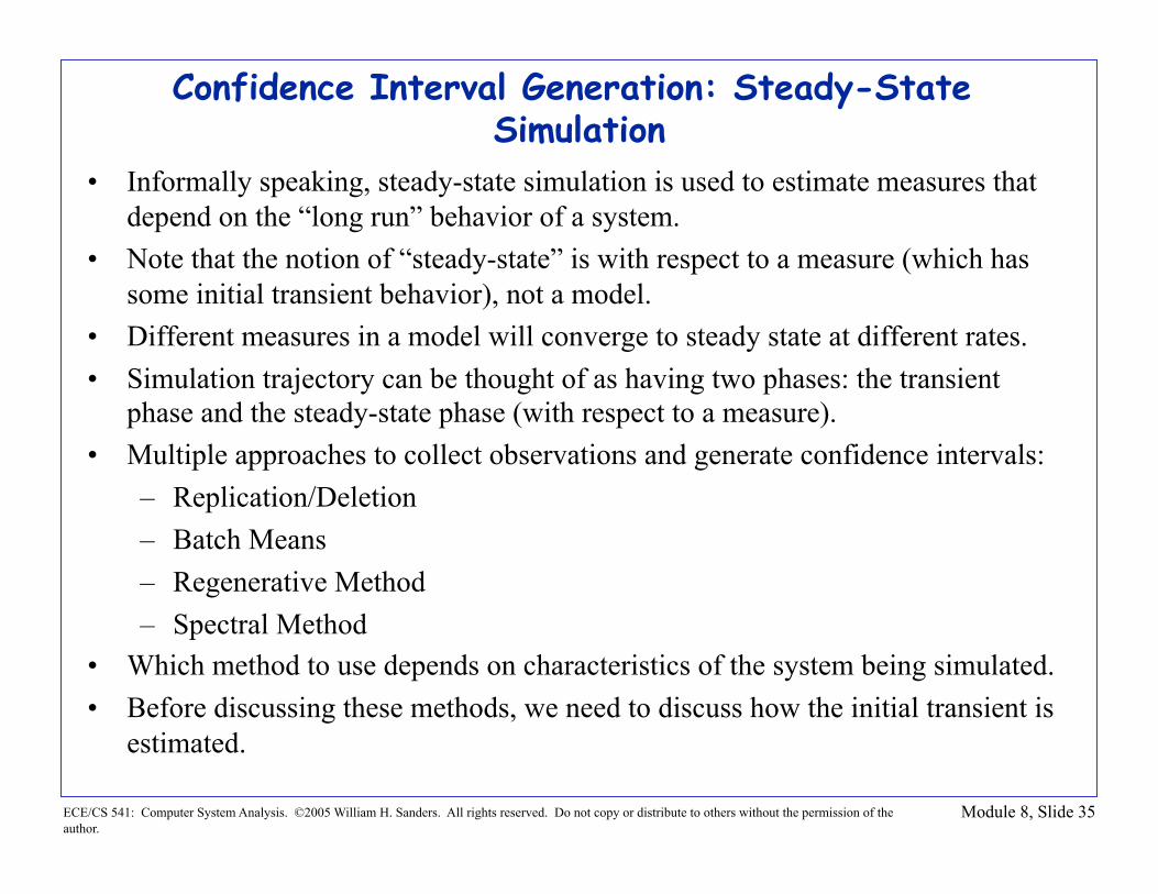
•  Informally speaking, steady-state simulation is used to estimate measures that depend on the “long run” behavior of a system.

•  Note that the notion of “steady-state” is with respect to a measure (which has some initial transient behavior), not a model.

•  Different measures in a model will converge to steady state at different rates. •  Simulation trajectory can be thought of as having two phases: the transient

phase and the steady-state phase (with respect to a measure). •  Multiple approaches to collect observations and generate confidence intervals:

–  Replication/Deletion –  Batch Means –  Regenerative Method –  Spectral Method

•  Which method to use depends on characteristics of the system being simulated. •  Before discussing these methods, we need to discuss how the initial transient is

estimated.


Estimating the Length of the Transient Phase

Problem: Observations of measures are different during so-called “transient phase,” and should be discarded when computing an estimator for steady-state behavior.

Need: A method to estimate transient phase, to determine when we should begin to collect observations.

Approaches: –  Let the user decide: not sophisticated, but a practical solution. –  Look at long-term trends: take a moving average and measure differences. –  Use more sophisticated statistical measures, e.g., standardized time series

(Schruben 1982).

Recommendation: –  Let the user decide, since automated methods can fail.


Methods of Steady-State Measure Estimation: Replication/Deletion

•  Statistics similar to those for terminating simulation, but observations collected only on steady-state portion of trajectory.

•  One or more observations collected per trajectory:

•  Compute

as ith observation, where Mi is the number of observations in trajectory i.

•  xi are considered to be independent, and confidence intervals are generated. •  Useful for a wide range of models/measures (the system need not be ergodic),

but slower than other methods, since transient phase must be repeated multiple times.

transient phase O11 O12

O21 O22

O31 O32 O33 O34

O23 O24

O13 O14 trajectory 1

trajectory 2

trajectory n

. . .

i

M

jij

i M

Ox

i

∑== 1


Methods of Steady-State Measure Estimation: Batch Means

•  Similar to Replication/Deletion, but constructs observations from a single trajectory by breaking it into multiple batches.

•  Example

•  Observations from each batch are combined to construct a single observation; these observations are assumed to be independent and are used to construct the point estimator and confidence interval.

•  Issues: –  How to choose batch size? –  Only applicable to ergodic systems (i.e., those for which a single trajectory

has the same statistics as multiple trajectories). –  Initial transient only computed once.

•  In summary, a good method, often used in practice.

initial transient O11 O12 O21 O22

O31 O32 O23

O13 11nO

33nO

22nO

...

... ... ...


Other Steady-State Measure Estimation Methods I •  Regenerative Method (Crane and Iglehart 1974, Fishman 1974)

–  Uses “renewal points” in processes to divide “batches.” –  Results in batches that are independent, so approach used earlier to generate

confidence intervals applies. –  However, usually no guarantee that renewal points will occur at all, or that

they will occur often enough to efficiently obtain an estimator of the measure.

•  Autoregressive Method (Fishman 1971, 1978) –  Uses (as do the two following methods) the autocorrelation structure of

process to estimate variance of measure. –  Assumes process is covariance stationary and can be represented by an

autoregressive model. –  Above assumption often questionable.


Other Steady-State Measure Estimation Methods II •  Spectral Method (Heidelberger and Welch 1981)

–  Assumes process is covariance stationary, but does not make further assumptions (as previous method does).

–  Efficient method, if certain parameters chosen correctly, but choice requires sophistication on part of user.

•  Standardized Time Series (Schruben 1983) –  Assumes process is strictly stationary and “phi-mixing.” –  Phi-mixing means that Oi and Oi + j become uncorrelated if j is large. –  As with spectral method, has parameters whose values must be chosen

carefully.


Summary: Measure Estimation and Confidence Interval Generation

1) Only use the mean as an estimator if it has meaning for the situation being studied. Often a percentile gives more information. This is a common mistake!

2) Use some confidence interval generation method! Even if the results rely on assumptions that may not always be completely valid, the methods give an indication of how long a simulation should be run.

3) Pick a confidence interval generation method that is suited to the system that you are studying. In particular, be aware of whether the system being studied is ergodic.

4) If batch means is used, be sure that batch size is large enough that batches are practically uncorrelated. Otherwise the simulation can terminate prematurely with an incorrect result.


Summary/Conclusions: Simulation-Based Validation Techniques

1) Know how random variates are generated in the simulator you use. Make sure: –  A good uniform [0,1] generator is used –  Independent streams are used when appropriate –  Non-uniform random variates are generated in a proper way.

2) Compute and use confidence intervals to estimate the accuracy of your measures. –  Choose correct confidence interval computation method based on the nature

of your measures and process

simulation basics - university of...

Documents