simulation and analysis of power system transients and... · · 2014-04-22wrocław university of...
TRANSCRIPT

Wrocław University of Technology
Control in Electrical Power Engineering
Marek Michalik, Eugeniusz Rosołowski
Simulation and Analysis of Power System Transients
Simulation and Analysis of Power System Transients
Wrocław 2010

Copyright © by Wrocław University of Technology Wrocław 2010
Reviewer: Mirosław Łukowicz
Project Office
ul. M. Smoluchowskiego 25, room 407 50-372 Wrocław, Poland Phone: +48 71 320 43 77
Email: [email protected] Website: www.studia.pwr.wroc.pl

CONTENTS
PREFACE................................................................................................................ 5 1. DISCRETE MODELS OF LINEAR ELECTRICAL NETWORK................... 7
1.1. Introduction ............................................................................................................ 7 1.2. Numerical solution of differential equations ......................................................... 8
1.2.1. Basic algorithms ........................................................................................................ 8 1.2.2. Accuracy of operation and stability ........................................................................... 12
1.3. Numerical models of network elements ................................................................ 14 1.3.1. Resistance.................................................................................................................. 14 1.3.2. Inductance ................................................................................................................. 14 1.3.3. Capacitance ............................................................................................................... 16 1.3.4. Complex RLC branches............................................................................................. 17 1.3.5. Controlled sources ..................................................................................................... 18 1.3.6. Frequency properties of discrete models ................................................................... 19 1.3.7. Distributed parameters model (long line model) ....................................................... 21
1.4. Nodal method ........................................................................................................ 28 1.4.1. Derivation of basic nodal equations........................................................................... 28 1.4.2. Simulation algorithm ................................................................................................. 31 1.4.3. Initial conditions........................................................................................................ 33
1.5. Numerical stability of digital models..................................................................... 35 1.5.1. Numerical oscillations in transient state simulations ................................................. 35 1.5.2. Suppression of oscillations by use of a damping resistance....................................... 37 1.5.3. Suppression of numerical oscillations by change of integration method ................... 40 1.5.4. The root matching technique ..................................................................................... 41
Exercises........................................................................................................................ 46 2. NON-LINEAR AND TIME-VARYING MODELS ......................................... 49
2.1. Solution of non-linear equations............................................................................ 49 2.1.1. Newton method ........................................................................................... 49
2.1.2. Newton–Raphson method ........................................................................................ 52 2.2. Models of non-linear elements .............................................................................. 53
2.2.1. Resistance................................................................................................................. 54 2.2.2. Inductance ................................................................................................................ 57 2.2.3. Capacitance .............................................................................................................. 59
2.3. Models of non-linear and time-varying elements .................................................. 60 2.3.1. Non-linear and time-varying scheme ....................................................................... 60 2.3.2. Compensation method.............................................................................................. 60 2.3.3. Piecewise approximation method............................................................................. 64
Exercises........................................................................................................................ 66

4 CONTENTS
3. STATE-VARIABLES METHOD ..................................................................... 67 3.1. Introduction ........................................................................................................... 67 3.2. Derivation of state-variables equations.................................................................. 69 3.3. Solution of state-variables equations ..................................................................... 72 Exercises........................................................................................................................ 74
4. OVER-HEAD LINE MODELS......................................................................... 75 4.1. Single-phase Line Model....................................................................................... 75
4.1.1. Line Parameters........................................................................................................ 75 4.1.2. Frequency-dependent Model .................................................................................... 77
4.2. Multi-phase Line Model ........................................................................................ 91 4.2.1. Lumped Parameter Model ........................................................................................ 91 4.2.2. Distributed Parameters Model.................................................................................. 98
Exercises........................................................................................................................ 111 5. TRANSFORMER MODEL............................................................................... 113
5.1. Introduction ........................................................................................................... 113 5.2. Single-phase Transformer...................................................................................... 114
5.2.1. Equivalent Scheme................................................................................................... 114 5.2.2. Two-winding Transformer ....................................................................................... 117 5.2.3. Three-winding Transformer ..................................................................................... 123 5.2.4. Autotransformer Model............................................................................................ 125 5.2.5. Model of Magnetic Circuit ....................................................................................... 126
5.3. Three-phase Transformer ...................................................................................... 132 5.3.1. Two-winding Transformer ....................................................................................... 132 5.3.2. Multi-winding Transformer...................................................................................... 140 5.3.3. Z (zig-zag)-connected Transformer.......................................................................... 145
Exercises........................................................................................................................ 148 6. MODELLING OF ELECTRIC MACHINES.................................................... 151
6.1. Synchronous Machines.......................................................................................... 151 6.1.1. Model in 0dq Coordinates ........................................................................................ 152 6.1.2. Model in Phase Coordinates..................................................................................... 168
6.2. Induction Machines ............................................................................................... 169 6.2.1. General Notes........................................................................................................... 169 6.2.2. Mathematical Model ................................................................................................ 171 6.2.3. Electro-mechanical Model ....................................................................................... 176 6.2.4. Numerical Models .................................................................................................... 180
6.3. Universal Machine................................................................................................. 181 Excersises ...................................................................................................................... 182
REFERENCES ........................................................................................................ 183 INDEX ..................................................................................................................... 189
PREFACE
The availability of modern digital computers has stimulated the use of computer simulation techniques in many engineering fields. In electrical engineering the computer simulation of dynamic processes is very attractive since it enables observation of electric quantities which can not be measured in live power system for strictly technical reasons. Thus the simulation results help to analyse the effects which occur in transient (abnormal) state of power system operation and also provide the valuable data for testing of new design concepts.
In case of computer simulation the continuous models have to be transformed into the discrete ones. The transformation is not unique since differentiation and integration may have many different numerical representations. Thus the selection of the numerical method has the essential impact on the discrete model properties. The basic difference between continuous and discrete models is observed in frequency domain: the frequency spectrum of signals in discrete models is the periodic function of frequency and the period depends on simulation time step applied. Another problem is related to numerical instability of discrete models which manifests itself in undamped oscillations even though the corresponding continuous models are stable. The arithmetic roundup affecting digital calculation accuracy may also contribute to the discrete models instability.
In this book all the aforementioned topics are concerned for discrete linear and nonlinear models of basic power system devices like: overhead transmission lines, cable feeders, transformers and electric machines. The relevant examples are presented with special reference to ATP-EMTP software package application.
We hope that the book will come in useful for both undergraduate and postgraduate students of electrical engineering when studying subjects related to digital simulation of power systems.
Wroclaw, September 2010 Authors

1. DISCRETE MODELS OF LINEAR ELECTRICAL NETWORK
1.1. Introduction
The simulation of power networks is aimed at detailed analysis of many problems and the most important of them are:
determination of power and currents flow in normal operating conditions of the network,
examination of system stability in normal and abnormal operating conditions, determination of transients during disturbances that may occur in the network, determination of frequency characteristics in selected nodes of the network.
The network model is derived from differential equations that relate currents and voltages in network nodes according to Kirchhoff’s law. The simulation models are usually based upon equivalent network diagrams derived under simplified assumptions (which sometimes can be significant) that are applied to the network elements representation. In this respect models can be divided into two basic groups: 1. Lumped parameter models. 3D properties of elements are neglected and
sophisticated electromagnetic relations that include space geometry of the network are not taken into account.
2. Distributed parameter models. Some geometrical parameters are used in the model describing equations (usually the line length). In classic theory relations between currents and voltages on the network elements
are continuous functions of time. In digital simulations the numerical approach must be applied. Two ways are applied for this purpose:
– transformation of continuous differential relations into discrete (difference) ones,
– state variable representation in continuous domain and its solution by use of numerical methods.
Consequences of transformation from continuous to discrete time domain: – problem of accuracy - discrete representations are always certain (more or less
accurate) approximation of continuous reality, – frequency characteristics become periodic according to Shannon’s theorem,

8 1. DISCRETE MODELS OF LINEAR ELECTRICAL NETWORK
– problem of numerical stability - numerical instability may appear even though the continuous representation of the network is absolutely stable.
1.2. Numerical solution of differential equations
1.2.1. Basic algorithms
In electric networks with lumped parameters the basic differential equation that describes dynamic relation between physical quantities observed in branches with linear elements (R, L, C) takes the form:
)()(d
)(d tbwtytty =+ λ (1.1)
where y(t), w(t) denotes electric quantities (current, voltage) and λ, b are the network parameters. In case of a single network component (inductor, capacitor) (1.1) simplifies into:
)(d
)(d tbwtty = (1.2)
Laplace transformation of (2) yields:
)()( sbWssY = (1.3)
To obtain discrete representation of (1.2) the continuous operator in s-domain must be replaced by the discrete operator z in z-domain (‘shifting operator’). The basic and accurate relation between those two domain is given by the fundamental formula:
sTez = (1.4)
where T - calculation step. Approximate rational relations between z and s can be obtained from expansions of
(1.4) into power series. Let’s consider the following three most obvious cases:
1. ......!)(...
!2)(1
2
+++++==n
TsTsTsezn
Ts (1.5)
Neglecting terms of powers higher than 1 results in approximation:
Tsz +≅ 1 (1.6)
and further:
T
zs 1−≅ (1.7)

1.2. Numerical solution of differential equations 9
2. Ts
TsTsTsez nTs
−=+++++≈=
11......)(...)(1 2 (1.8)
Again, if the higher power terms are neglected then:
Ts
z−
≅1
1 (1.9)
and
Tz
zs 1−≅ (1.10)
3. sTez = (1.11)
⎥⎦
⎤⎢⎣
⎡+
+−+
+−== ......
)1(3)1(
112ln1
3
3
zz
zz
Tz
Ts (1.12)
Again, if terms of power higher than 1 are neglected then:
)1()1(2
+−≅
zTzs (1.13)
The approximation (1.13) is the well known Bilinear Transformation or Tustin’s operator.
Applying the derived approximations of s to differential equation (1.3) three different discrete algorithms for numerical calculation of w(k) integral can be obtained.
Using the first approximation of s (1.7) in (1.3):
)()(1 zbWzYT
z =− (1.14)
and, in discrete time domain:
)()()1( kbwT
kyky =−+ (1.15)
The obtained formula (1.15) is the Euler’s forward approximation of a continuous derivative. The corresponding integration algorithm takes the form:
)()()( 11 zbTWzzYzzY −− += (1.16)
and

10 1. DISCRETE MODELS OF LINEAR ELECTRICAL NETWORK
)1()1()( −+−= kbTwkyky (1.17)
The algorithm (1.17) realizes iteration that within a single step T can be written as:
ττ d)()()(1
1 ∫−
+= −
k
k
t
tkk wbTtyty (1.18)
The algorithm (1.17) is of explicit type since the current output in k-th calculation step depends only on past values of the input and output in (k–1) instant.
Using the second approximation of s (1.6):
)()(1 zbWzYzT
z =− (1.19)
and
)()1()( kbwT
kyky =−− (1.20)
Now the obtained formula (1.20) is the Euler’s backward approximation of a continuous derivative. The resulting integration algorithm takes the form:
)()()( 1 zbTWzYzzY += − (1.21)
and
)()1()( kbTwkyky +−= (1.22)
This algorithm is of implicit type since the current output in k-th instant depends on present value of the input in the same instant.
The algorithm (1.9) which realizes integration within a single step T, can now be written as:
ττ d)()()(1
1 ∫+
+= −
k
k
t
tkk wbTtyty (1.23)
Using the third approximation of s (1.7) in (1.3) we get:
)()()1()1(2 zbWzY
zTz =
+−
(1.24)
( )
2)()()()(
11 zWzzWTbzYzzY
−− ++= (1.25)

1.2. Numerical solution of differential equations 11
( )
2)1()()1()( −++−= kwkwTbkyky (1.26)
This algorithm (1.26) realizes numerical integration based upon trapezoidal approximation of the input function w(k).
Graphical representation of all derived integrating algorithms is shown in Fig.1.1.
Fig.1.1. Numerical integration; 1 - Euler’s ‘step back’ (explicit) approximation.;2 - Euler’s ‘step forward’ (implicit) approx.; 3 - trapezoidal approximation
Examination of Fig.1.1 leads to the following conclusions: Forward approximation of derivative results in ‘step backward’ (explicit)
integrating algorithm and vice versa. The explicit algorithm tends to underestimate while the implicit one overestimates the integration result.
The algorithm based on trapezoidal approx. reduces the integration error since its output yTR(k) (1.10) is an average of outputs of both aforementioned algorithms yE(k) (1.8), yI(k) (1.10) at any instant k, i.e.
2
)()()( kykyky IETR
+= (1.27)
In general, the numerical integration methods depend on approximations of continuous derivative (or integral) and can be divided into two groups, namely:
– single step integration methods (self-starting), – multi-step methods. All algorithms considered belong to the first group. As an example of a multi-step
numerical integrator the 2-nd order Gear algorithm can be shown:

12 1. DISCRETE MODELS OF LINEAR ELECTRICAL NETWORK
3
)()2()1(4)( kTbwkykyky +−−−= (1.28)
The algorithm is not self-starting one and must be started by use of a single step algorithm but reveals stiff stability properties.
1.2.2. Accuracy of operation and stability
Accuracy of numerical integration for the algorithms considered can be estimated from homogenous form of the eqn.(1.1), i.e.:
0)(d
)(d =+ tytty λ (1.29)
which yields the accurate solution:
tetyty λ−= )()( 0 (1.30)
where y(t0) – initial condition at t0 ; λ >0 Applying s approximations (1.7, 1.10, 1.13) to (1.29) the following numerical
expressions are obtained [18]: – Explicit Euler’s method (‘step backward’) (1.7)
)1()1()( −−= kyTky λ (1.31)
– Implicit Euler’s method (‘step forward’) (1.10)
T
kykyλ+−=
1)1()( (1.32)
– Trapezoidal approximation (1.13)
)1(22)( −
+−= ky
TTky
λλ
(1.33)
Accurate result of integration at the instant tk=kT is:
TaL ekyky λ−−= )1()( (1.34)
Thus the local integration error for one interval T=tk– tk-1 can be defined as:
)()( kykyaLL −=Δ (1.35)
This local error can easily be determined for each algorithm considered. Let’s take for example the method (1.7):

1.2. Numerical solution of differential equations 13
)1)(1()1()1()1( TekykyTeky TTL λλ λλ +−−=−−−−=Δ −− (1.36)
Expansion of the exponential term into power series yields:
.....)
!3)(
2)()(1(
32
+−−=Δ TTkyLλλ
(1.37)
Putting the constraint λT < 1 and using some mathematics the local error can be estimated by the approximate formula:
)2()2(
)(1
1
TT
p
p
L λλ
+=Δ −
+
(1.38)
where p is the order of the algorithm(in this case p = 1). The global error ΔG is defined as the difference between accurate and approximate
integration result in a longer time span i.e. from the first step (k = 1) to the arbitrary step k > 1 so that:
)(0 kyey TkG −=Δ − λ (1.39)
The respective integration results of (1.29) for the algorithms considered are (order of presentation as in previous case):
– Explicit Euler’s method (‘step backward’) (1.7):
0)1()( yTky kλ−= (1.40)
– Implicit Euler’s method (‘step forward’) (1.10):
kTyky
)1()( 0
λ+= (1.41)
– Trapezoidal approximation (1.13):
022)( y
TTky
k
⎥⎦⎤
⎢⎣⎡
+−=
λλ
(1.42)
Discussion of results
Algorithms (1.31) and (1.40). The integration method is convergent and the algorithms remain stable if:
11 <− Tλ (1.43)
Thus, the stability of the algorithms is ensured if:

14 1. DISCRETE MODELS OF LINEAR ELECTRICAL NETWORK
λ2<T (1.44)
The remaining algorithms are stable regardless of the value of T. If the algorithm is stable the global error tends to zero even though the local
error may attain significant values. Illustration of the errors discussed is shown in Fig.1.2. The plots presented have
been calculated for: y0 = 10; λ = 2; T = 0.987 [76].
–2
–1
0
1
2
3
ΔL
1
2
3
T, s
–10
–5
0
5
10
0 4 8 12 16 20k
31
2
ΔG
a) b)
10–4 10–3 10–2 10–1 100
Fig. 1.2. Local ΔL and global ΔG error values for the algorithms considered: 1 – trapezoidal approx.; 2 – Euler’s ‘step forward’ ; 3 – Euler’s ‘step backward’
1.3. Numerical models of network elements
1.3.1. Resistance
As the resistive elements do not have the energy storing capacity the discrete relation between current and voltage drop across resistance R can be obtained directly from the continuous relation and:
)()(1)( kGukuR
ki == (1.45)
1.3.2. Inductance
The energy stored in magnetic field produced by current has the impact on voltage across the element so its continuous model is described by the equation:
)(1d
)(d tuLt
ti = (1.46)

1.3. Numerical models of network elements 15
Using the transformation (1.6) or (1.9) the Euler’s implicit discrete model of the element is obtained:
LTGkGukiku
LTkiki =+−=+−= ),()1()()1()( (1.47)
Note that T/L has the conductance unit. For the trapezoidal transformation (1.7) or eqn.(1.10) the discrete model takes the
form:
[ ])()1(2
)1()( kukuL
Tkiki +−+−= (1.48)
or
L
TGkGukikGuki2
),1()1()()( =−+−+= (1.49)
The eqn. (1.49) can be rearranged in the following way:
)1()1()()( −+−+= kGukikGuki (1.50)
or
)1()()( −+= kjkGuki (1.51)
where
)1()1()1( −+−=− kGukikj (1.52)
The calculations in step k employ the values calculated in step k–1 which are constant and can be considered as the constant current sources j(k–1). Thus the inductance can be represented by equivalent numerical model corresponding to (1.52) which is shown in Fig.1.3.
a)
u(k)
i(k)
G j(k-1)i(t)
u(t)
L
b)
Fig. 1.3. Discrete model of inductance; a) symbol; b) numerical model

16 1. DISCRETE MODELS OF LINEAR ELECTRICAL NETWORK
1.3.3. Capacitance
This element also reveals the energy storing capacity in form of electric charge and the relation between voltage and current in the element is given by the formula:
)(1d
)(d tiCt
tu = (1.53)
Using the same transformations as for the inductance the discrete models of capacitance can be derived:
)()1()( kiCTkuku +−= (1.54)
Introducing the conductance notation (1.54) takes the form:
TCGkGukGuki =−−= ),1()()( (1.55)
and
)1()1(),1()()( −−=−−+= kGukjkjkGuki (1.56)
Using the trapezoidal integration method the discrete model of capacitance takes the similar form:
( ))()1(2
)1()( kikiCTkuku +−+−= (1.57)
The companion discrete model for capacitance can be derived as:
)1()()( −+= kjkGuki (1.58)
TCGkGukikj 2),1()1()1( =−+−−=− (1.59)
The respective representation is shown in Fig.1.4:
u(k)
i(k)
G j(k-1)i(t)
u(t)
C
a) b)
Fig. 1.4. Discrete model of capacitance; a) symbol; b) numerical model

1.3. Numerical models of network elements 17
In the very similar way the parameters of circuit representations for any integration method used can be derived. In Table 1.1 the example of those parameters for three selected methods are shown.
Table 1.1. Companion circuit parameters for selected numerical integration methods.
Integration method Model of inductance L Model of capacitance C Euler’s implicit
method )1()1( −=− kikj ,
LTG = )1()1( −−=− kGukj ,
TCG =
Trapezoidal approximation
)1()1()1( −+−=− kGukikj , L
TG2
= ( ))1()1()1( −+−−=− kGukikj , TCG 2=
Gear’s 2nd order ( ))2()1(4
31)1( −−−=− kikikj ,
LTG
32=
⎟⎠⎞
⎜⎝⎛ −+−−=− )2(
31)1(2)1( kukuGkj
TCG
23=
Basic numerical algorithm: )1()()( −+= kjkGuki
1.3.4. Complex RLC branches
The equivalent discrete model of in series connected RLC branch can be obtained by series connection of basic models of each particular element in the branch as it is shown in Fig.1.5b.
u(k)
GR
i(t)
uR(t)
L
a) b)
jC(k-1)C
c)
R
GL
GC
uL(t)
uC(t)
jL(k-1) j(k-1)G
i(k)
i(k)
uR(k)
uL(k)
uC(k)
u(t)
Fig. 1.5. Discrete model of RLC branch; a) the continuous model; b) discrete models of particular elements; c) the equivalent discrete model of the branch.

18 1. DISCRETE MODELS OF LINEAR ELECTRICAL NETWORK
To derive the equivalent discrete model (Fig. 1.5c) of the overall circuit consider the basic equation for voltage across the branch (Fig. 1.5b):
)()()()( kukukuku CLR ++= (1.60)
in which the particular terms can be expressed by their basic models:
( ) ( ).)1()(1)(,)1()(1)(
),(1)(
−−=−−=
=
kjkiG
kukjkiG
ku
kiG
ku
CC
CLL
L
RR
(1.61)
After substitution and appropriate rearrangement of (1.60) the equivalent model equation is obtained:
)1()()( −+= kjkGuki (1.62)
in which, for trapezoidal approximation:
2242
TRCTLCCT
GGGGGGGGGG
CLCRLR
CLR
++=
++=
)1()1()1()1()1( −+−=++
−+−=− kjGGkj
GG
GGGGGGkjGGkjGGkj C
CL
LCLCRLR
CLRLCR ,
and R
GR1= ,
LTGL 2
= , TCGC
2= .
If capacitance C is not present in a branch then C→∞ must be put into the above equations. For missing R or L, R = 0 or L = 0 must be used, respectively. For example, in case of the R L branch the respective relations are:
RTL
TG+
=2
)1()1(11)1(
22)1( −+−
+−=−
+=− kGuki
RGRGkj
RTLLkj
L
LL (1.63)
1.3.5. Controlled sources
Controlled sources are used very often in electronic and electric network models. Generally there are four basic types of such sources (Fig.1.6) [18, 70]:
Voltage controlled current sources xkuj = controlled by voltage xu applied to control terminals.
Current controlled current sources xkij = controlled by current xi injected into control terminals.
Voltage controlled voltage sources xkuu = .

1.3. Numerical models of network elements 19
Current controlled voltage sources xkiu = .
j=kuxux
u=kix
ix
j=kix
ix
u=kuxux
a) b)
c) d)
Fig. 1.6. Diagrams of controlled sources; a) voltage controlled current source; b) current controlled current source; c) current controlled voltage source;
d) voltage controlled voltage network.
Models of controlled sources are very simple; however, their implementation in simulation programs may sometimes be cumbersome.
1.3.6. Frequency properties of discrete models
The frequency properties of discrete models are uniquely determined by the method used for approximation of derivatives that appear in the continuous model of a given element. Comparison of the continuous and the discrete models frequency properties provides very useful information on how to select the calculation period T in order to obtain the accurate enough transient component waveform of specified frequency fmax which is present in the frequency spectrum of continuous transient voltages or currents.
As an example let’s consider the discrete model of inductance obtained by use of trapezoidal approximation. Using the already known relations (1.46, 1.13) we get:
)(1)()1()1(2 zu
Lzi
zTz =
+− (1.64)
)(11
2)( zu
zz
LTzi
−+= (1.65)
Now using (1.4) and remembering that in frequency domain s=jω :
)j(11
2)j( j
j
ωω ω
ωu
ee
LTi T
T
−+= (1.66)

20 1. DISCRETE MODELS OF LINEAR ELECTRICAL NETWORK
Applying rudimentary trigonometry knowledge the magnitude of the equation (1.66) can be written in the following form:
)j(
2tan
2)j( ωωω uTL
T
i = (1.67)
Introducing the complex discrete admittances Yd(jω) and the continuous Yc(jω) we get:
)j(
2tan
2
2tan2
2tan
2)j()j(
)j( ωω
ω
ωω
ω
ωωω
ω cd YT
T
TL
T
TL
T
ui
Y ==== (1.68)
where Yc(jω) = 1/jLω is the admittance of the continuous model of inductance. Thus, the ratio of the discrete admittance to the continuous one is given by:
2tan
2)j()j(
T
T
YY
c
d
ω
ω
ωω
= (1.69)
and changes with frequency as it is shown in Fig. 1.7.
0 0.1 0.2 0.3 0.4 0.50
0.1
0.2
0.3
0.4
0.5
0.6
0.7
0.8
0.9
πω2
T
YYd
Fig. 1.7. Frequency response of discrete inductance model.

1.3. Numerical models of network elements 21
From eqn. (1.69) and from Fig. 1.7 one can notice that Yd(jω) reaches zero if
∞→2
tan Tω This limit is reached when:
ff
TorT21
222====
ππ
ωππω (1.70)
So if fmax is the frequency of the highest harmonic to be observed in current or voltage signals then the calculation step T should be small enough according to following condition:
max21f
T << (1.71)
Practically, if required number of data samples within the period max
max fT 1= is N
then (1.71) implies:
max
1Nf
T ≤ (1.72)
in which N must not be less than 2 (usually N > 20).
1.3.7. Distributed parameters model (long line model)
Distinction between lumped and distributed models of electric elements is made on the basis of mutual relation between three basic parameters of the environment in which the electromagnetic wave is propagated. These parameters are:
specific electric conductivity γ relative magnetic permeability μ relative electric permittivity ε
In case of lumped elements it is assumed that only one of the above listed parameters is dominant and the remaining ones can be neglected. Thus particular elements are deemed as lumped under following conditions:
μ = ε = 0 – lumped resistance γ = ε = 0 – lumped inductance γ = μ = 0 – lumped capacitance.
Additionally in case of lumped parameters model of an electric network the electromagnetic field must be quasi-stationary; it means that in each point of the network the electromagnetic field is practically the same or the differences are negligibly small. In this respect the length of the electric conductor l is considered as
22 1. DISCRETE MODELS OF LINEAR ELECTRICAL NETWORK
the distinctive parameter. As the boundary value the length lgr equal to ¼ of the electromagnetic wavelength propagated is assumed.
Thus, if the frequency of the propagated wave is f, than the lgr can be estimated as:
f
clgr 44== λ , (1.73)
where c is the velocity of light and fc=λ is the wavelength.
If grll << then the length of the line can be neglected and can be modelled as the lumped parameter element. Otherwise ( grll ≈ ) the line should be considered as the long one.
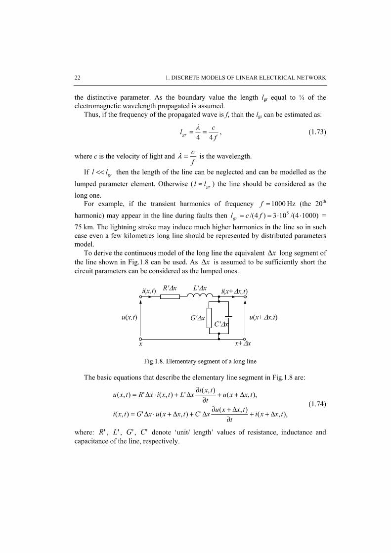
For example, if the transient harmonics of frequency 1000=f Hz (the 20th harmonic) may appear in the line during faults then )10004/(103)4/( 5 ⋅⋅== fclgr = 75 km. The lightning stroke may induce much higher harmonics in the line so in such case even a few kilometres long line should be represented by distributed parameters model.
To derive the continuous model of the long line the equivalent xΔ long segment of the line shown in Fig.1.8 can be used. As xΔ is assumed to be sufficiently short the circuit parameters can be considered as the lumped ones.
R'Δx L'Δx
G'ΔxC'Δx
u(x,t) u(x+Δx,t)
i(x,t) i(x+Δx,t)
x x+Δx
Fig.1.8. Elementary segment of a long line
The basic equations that describe the elementary line segment in Fig.1.8 are:
),,(),('),('),(
),,(),('),('),(
txxit
txxuxCtxxuxGtxi
txxut
txixLtxixRtxu
Δ++∂
Δ+∂Δ+Δ+⋅Δ=
Δ++∂
∂Δ+⋅Δ= (1.74)
where: 'R , 'L , 'G , 'C denote ‘unit/ length’ values of resistance, inductance and capacitance of the line, respectively.

1.3. Numerical models of network elements 23
Dividing both equations by xΔ and taking the limes ( 0→Δx ) the following relations are obtained:
.),('),('),(
,),('),('),(
ttxuCtxuG
xtxi
ttxiLtxiR
xtxu
∂∂+=
∂∂−
∂∂+=
∂∂−
(1.75)
If the line is homogenous then (1.75) can be separated with respect to current and voltage (for simplicity: ),( txuu = , ),( txii = ):
tx
iLtuCRuGR
xu
∂∂∂+
∂∂−−=
∂∂−
2
2
2
''''' (1.76)
and
( ) 2
2
2
2
''''''''tuCL
tuLGCRuGR
xu
∂∂+
∂∂++=
∂∂ (1.77)
Applying the same simplifying procedure to the second equation in (1.75) the
respective relation for current can be obtained:
( ) 2
2
2
2
''''''''tiCL
tiLGCRiGR
xi
∂∂+
∂∂++=
∂∂ (1.78)
Both (1.75) and (1.76) are the second order hyperbolic partial differential equations known as telegraph equations [80].
a) Lossless (non-dissipating) long line
This case is obtained under assumption that 0'=R and 0'=G and the resulting simplification of (3.4) and (3.5) is:
.01
,01
2
2
22
2
2
2
22
2
=∂∂−
∂∂
=∂∂−
∂∂
ti
vxi
tu
vxu
(1.79)
in which:
''
1CL
v = (1.80)

24 1. DISCRETE MODELS OF LINEAR ELECTRICAL NETWORK
The general solution of (3.6) has been found by d’Alembert [24, 28]. For the following boundary conditions:
)(),( 0 ttxu x ϕ== , )(),(
0t
xtxu
xψ=
∂∂
=
the solution of (1.79) takes the form:
( ) ∫+
+−++=x/vt
x/v-td)(
2)/()/(
21),( ααψϕϕ vvxtvxttxu (1.81)
The loci of points const)/( =− vxt and const)/( =+ vxt known as propagation characteristics of (1.81) [6, 39] show the propagation mechanism of ),( txϕ waves in a long line.
x
t
x1 x2xp
tp
t-x/v=constt+x/v=const
Fig. 1.9. Propagation characteristics of a lossless long line
The boundary conditions expressed in terms of voltage )(1 tu and current )(1 ti at the beginning of the lossless ( 0=R' ) line (1.75) yields:
)(),0()( 1 tutut ==ϕ , ttiL
ttiL
xtut
d)(d'),0('),0()( 1−=
∂∂−=
∂∂=ψ
and the solution (1.81) takes the form:
( ) ∫+
−−++=x/vt
x/v-t11 )(d21)/()/(
21),( tiZvxtuvxtutxu if (1.82)
where ''
CLZ f = is the wave (surge) impedance of the line.
For lx = (end of the line) solution of (1.82) is given by the equation:
1.3. Numerical models of network elements 25
( ) ( ))()(21)()(
21)( 11112 ττττ −−+−−++= titiZtututu f (1.83)
where: vl /=τ is the line propagation time. Similarly, the wave equation for current can be obtained and:
( ) ( ))()(2
1)()(21)( 11112 ττττ −−++−++−= tutu
Ztititi
f (1.84)
Note that it was assumed that the current at the end of the line flows in reverse direction with respect to the current at the line beginning (see Fig.1.8) and that is why it bears the opposite sign.
Subtracting (1.83) from (1.84) the model of the long lossless line is obtained:
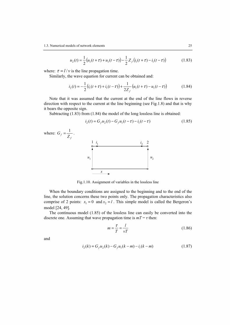
)()()()( 1122 ττ −−−−= tituGtuGti ff (1.85)
where: f
f ZG 1= .
u1 u2
i1 i2 21
x
Fig.1.10. Assignment of variables in the lossless line
When the boundary conditions are assigned to the beginning and to the end of the line, the solution concerns these two points only. The propagation characteristics also comprise of 2 points: 01 =x and lx =2 . This simple model is called the Bergeron’s model [24, 49].
The continuous model (1.85) of the lossless line can easily be converted into the discrete one. Assuming that wave propagation time is mT = τ then:
vTl
Tm == τ (1.86)
and
)()()()( 122 mkimkuGkuGki iff −−−−= (1.87)

26 1. DISCRETE MODELS OF LINEAR ELECTRICAL NETWORK
By analogy the discrete model for the current at the beginning of the line can be derived, so the respective input and output line currents are:
),()()(
),()()(
222
111
mkjkuGki
mkjkuGki
f
f
−+=
−+= (1.88)
where
),()()(
),()()(
112
221
mkimkuGmkj
mkimkuGmkj
f
f
−−−−=−
−−−−=− (1.89)
The equivalent circuits corresponding to (1.88) and (1.89) are shown in Fig. 1.11.
u1(k)
1 i1(k)
Gf
j1(k-m)u2(k)
2i2(k)
Gf
j2(k-m)
Fig.1.11. Equivalent circuit of the long line discrete model
b) The long line model with dissipation losses
The dissipation losses are uniquely attributed to heating of the line resistance which was neglected in derivation of the lossless line model. The inclusion of the resistance to the long line model is based upon assumption that its value is relatively small with respect to the line reactance. This assumption justifies the inclusion of the lumped resistance at both ends of the line as it is shown in Fig. 12.
When the resistance is connected as shown in Fig.1.12a the equations (1.88), (1.89) refer to voltages at nodes 1’and 2’ for which the following relations are valid:
),(
2)()('
),(2
)()('
222
111
kiRkuku
kiRkuku
−=
−= (1.90)
where: 'lRR = As the result the conductance fG and history of calculation changes so that:
),()()(
),()()(
112
221
mkihmkuGmkj
mkihmkuGmkj
ff
ff
−−−−=−
−−−−=− (1.91)

1.3. Numerical models of network elements 27
where:
2/1
RZG
ff +
= , RZRZ
hf
ff +
−=
22
.
a)
b)
u1(k)
1 i1(k) R/2
u2(k)
2i2(k)R/2
u'2(k)u'1(k)
1' 2'
u1(k) u2(k)
1R/4
2R/4R/4 R/4i1(k) i2(k)
R/2
Fig.1.12. Inclusion of resistance into the long line model
More accurate model can be obtained when the resistance is connected into the line model as it is shown in Fig.1.12b. In this case all the line parameters connected to the middle node of the line can be eliminated and the resulting equations obtained are:
),()()()(
),()()()(
1222
2111
mkjhmkjhkuGki
mkjhmkjhkuGki
fbfaf
fbfaf
−+−+=
−+−+= (1.92)
where: fffa GZh = , ffb GRh4
= , and 4/
1RZ
Gf
f += .
In general the dissipating long line models can be written in the compact matrix form so that:
⎥⎦
⎤⎢⎣
⎡−−
⎥⎦
⎤⎢⎣
⎡+⎥
⎦
⎤⎢⎣
⎡⎥⎦
⎤⎢⎣
⎡=⎥
⎦
⎤⎢⎣
⎡)()(
)()(
)()(
2
1
2
1
2
1
mkjmkj
hhhh
kuku
GG
kiki
fafb
fbfa
f
f (1.93)

28 1. DISCRETE MODELS OF LINEAR ELECTRICAL NETWORK
and the matrixes ff G=G and ff h=h . The form of the matrixes depends upon the considered representation of the
dissipating long line (as in Fig. 1.12a or as in Fig. 1.12.b).
1.4. Nodal method
The method is frequently used for network node equations formulation mainly because its application is easy and the algorithms of nodal equations solution are well known and fast. Below, the fundamentals of nodal method are presented which refer to the admittance representation of network branches with current and voltage controlled sources. Extension of the method for networks containing voltage and current controlled voltage sources branches is known as the modified nodal method and will not considered here since the method is mainly applied to simulation of transients in electronic networks [8, 36].
1.4.1. Derivation of basic nodal equations
The equivalent diagram of the network branch typical for the nodal method is shown in Fig.1.13. The mathematical model of the branch is described by the following equation:
anmbalkaabbaaaa juuGuuGjuGuGi +−+−=++= )()( (1.94)
where bu is the current source controlling voltage with the control coefficient baG , located in the other network branch It must be noted that aj may refer to the independent current source as well as to the source related to the past values of current (history) in the branch.
ua
ja
Gia
Gbaub
k l
Fig. 1.13. Equivalent diagram of the conductance branch typical for nodal method
Let's consider a network comprising of gn branches and 1+wn nodes with one of the nodes being the reference one. Such a network can be described by equation (1.94) written in matrix form:

1.4. Nodal method 29
gT
gg juAGi += (1.95)
where: – ( )gg nng ×
G is the conductance matrix which contains branch conductances aG (at
the diagonal) and conductances of controlled current sources baG (outside the diagonal);
– gw nn ×A = aij is the incidence matrix which takes the following values : 1=ija
– if the branch j is connected to the node i and is directed to that node, 1−=ija – if the branch is of opposite direction, 0=ija – if the branch j is not
connected to the node i ; – u is the vector of potentials in wn independent network nodes (it is the vector
of voltage difference between particular nodes and the reference node); – gj is the vector of nodal current sources.
Multiplication of (1.94) by the incidence matrix A transforms the branch currents into the nodal ones. The sum of the branch currents in each node is always equal to zero (the first Kirchhoff’s law) so that:
0=gAi (1.96)
and, for the right side of (1.94): iGu = (1.97)
where: Tgnn ggAAGG =× is the matrix of nodal conductance , gnw
Aji −=×1 is the
vector of the nodal currents (positive sign is assigned to elements of the vector i if the corresponding source is directed to the node).
Due to the matrix A definition particular elements of the vector i are the sum of branch currents which are directed to a given node.
Relation (1.97) is known as the equation of nodal potentials. For a given matrix G and for the known excitation vector i solution of (1.97) yields the vector u which determines voltages between the independent nodes and the reference one. To facilitate the network transient calculations some modifications are applied to (1.97). Two such modifications are of extreme importance in power system networks calculations since they enable:
– inclusion of voltage sources connected to the reference node; – improvement of calculation in case of parameter changes in selected branches. If independent voltage sources connected in series with impedance appear in
branches then they should be transformed into the equivalent current sources according to the Norton's theorem. In power networks the reference node is usually

30 1. DISCRETE MODELS OF LINEAR ELECTRICAL NETWORK
assigned to earth In such case all voltage sources connected to earth are no longer independent. To avoid this the following procedure can be applied [24, 87]:
• Select the set of nodes A (excluding the reference node) for which nodal voltages are not determined.
• Nodes with determined voltages belong to the set B. The sum of both set makes the total set of all independent nodes in the network: BAw nnn += .
• Vector of nodal voltages u in (1.97) can now be presented as:
⎥⎦
⎤⎢⎣
⎡=
B
A
uu
u (1.98)
in which only the vector Au is to be determined. • Now (1.97) can be written as:
⎥⎦
⎤⎢⎣
⎡=⎥
⎦
⎤⎢⎣
⎡⎥⎦
⎤⎢⎣
⎡
B
A
B
A
BBBA
ABAA
ii
uu
GGGG
(1.99)
where: AAG is the conductance matrix of that part of the network which has no nodes connected to the branches with voltage sources, BBG contains self and mutual conductances of nodes for which voltages are known, while ABG and
BAG represent matrixes of mutual conductances of sets A and B; node current vector is divided similarly.
• The unknown node voltage vector Au can be determined from the equation:
BABAAAA uGiuG −= (1.100)
while the node current vector in the set B can be found from the lower part of (1.99):
BBBABAB uGuGi += (1.101)
Elements of the vector Bi are the sum of sources current flowing into the respective nodes in the set B, including branches obtained for the voltage sources.
Another important issue related to calculation of transients is the possibility of an easy change of network configuration without necessity of matrix G calculation. This problem appears, for instance, when switches in the network being analyzed change their positions. In such case any switch can be represented by the conductance branch for which the value of wylG depends upon the switch position: maxwyl FG = – the
switch closed, 0wyl =G – the switch open; maxF – very big real value. Thus, when the switches change position the overall network configuration remains unchanged, only

1.4. Nodal method 31
the values of matrix G elements change. That is why the nodes connected to the switch branches should be located in lower part of matrix G [22]. The example illustrating the nodal method application is shown in [76].
In existing simulation programs the Gaussian elimination method is applied in versions which differ mainly in representation of elements with variable parameters (switches). It should be noted that the representation of a switch by the element of variable conductance may bring about some numerical problems when the conductance value is very small (closed switch) since the matrix may become singular.
1.4.2. Simulation algorithm
The detailed algorithm of transient simulation depends mainly upon how the numerical problems are solved. However, in general, all algorithms comprise of the three basic stages (Fig. 1.14):
Yes
Data inputSet initial conditions
t=0
Set up matrix G(the upper triangular part of the matrix)
Set up the lower partof the triangular matrix G
Switch position change?
Determine vector of source currentsfor independent sources and history
No
Calculate node voltages: reversesubstitution (Gauss method)
Determine output
t=t+T
t>tmax?
Output file
StopNo
Yes
Fig. 1.14. Basic structure of algorithms for transient calculation using the nodal method

32 1. DISCRETE MODELS OF LINEAR ELECTRICAL NETWORK
• Data and initial conditions setup • Calculations • Results record
The results of the algorithm operation can be illustrated by the following example.
Example 1.1. Simulate the transients generated in the network shown in Fig.1.15a which is the part of the 400 kV power system drawn for the positive sequence impedances. Assume that all current and voltage initial conditions for (t<0) are equal to zero.
System parameters: sE = 330 kV, sZ = 0.5 + j10 Ω, 1Z = 4700 + j2800 Ω, 2Z = 415 + j200 Ω.
Line: 'R = 0.0288 Ω/km, 'L =1.0287 mH/km, 'C =11.232 nF/km, length l =180 km. Calculation step: T = 5⋅10–5 s. Using the respective digital models for the system elements the equivalent network shown in Fig.1.15b is obtained. The switch W is closed (GW = 106 S). Simulation starts (t = 0) when the voltage ES is switched on.
jZs(k–1)
GZs
es(k)
1
jL1(k–m)
GfjZ1(k–1)GZ1
jL2(k–m)Gf
jZ2(k–1)
GZ2
2 4is(k)iZ1(k)
iL1(k) iL1(k)iZ2(k)
GW 3 b)
Fig.1.15. Illustration of the simulation algorithm operation; a) analyzed system; b) equivalent network of the analyzed system
Simulation is based on step by step solving of (1.100) and (1.101).The selected waveforms of currents and voltages in the network are shown in Fig. 1.16. The intensive transient state caused by charging of the line can be noticed in the first period of fundamental frequency. The oscillation period is equal to the propagation time necessary for the electromagnetic wave to travel along the line in both directions. Relatively slow decay of those oscillations can partly be attributed applied trapezoidal integration method which is
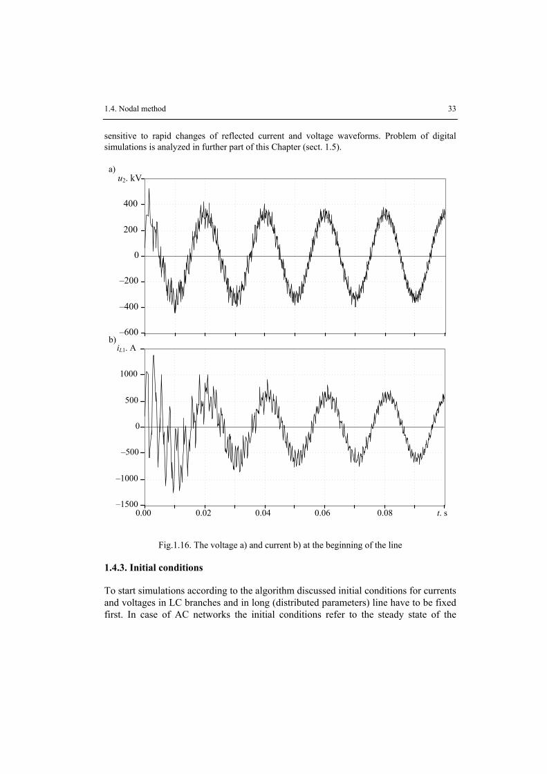
1.4. Nodal method 33
sensitive to rapid changes of reflected current and voltage waveforms. Problem of digital simulations is analyzed in further part of this Chapter (sect. 1.5).
–1500
–1000
–500
0
500
1000
iL1. A
0.00 0.02 0.04 0.06 0.08 t. s
–600
–400
–200
0
200
400
u2. kVa)
b)
Fig.1.16. The voltage a) and current b) at the beginning of the line
1.4.3. Initial conditions
To start simulations according to the algorithm discussed initial conditions for currents and voltages in LC branches and in long (distributed parameters) line have to be fixed first. In case of AC networks the initial conditions refer to the steady state of the

34 1. DISCRETE MODELS OF LINEAR ELECTRICAL NETWORK
network before calculation of transients starts. Thus, the initial conditions are determined for complex network model with sinusoidal excitation sources and with all switches set to positions corresponding to the network normal operating conditions.
If the network includes nonlinear elements then, initial conditions calculations are carried out for linear approximation of their nonlinear transition characteristics. In case of long lines which are modelled as elements of distributed parameters initial conditions are calculated using the simplified model in which the line is represented by a single Π cell as it is shown in Fig. 1.17.
1
ppY21
LY 21I 2I
ppY21
Fig. 1.17. Equivalent circuit of along line for steady state calculations
The values of admittances in the circuit shown in Fig. 1.17 can be determined from 'unit per length' parameters of the line according to the following equations:
LL Z
Y 1= , where: ( )l
lL'R'lZ L γγω sinhj+= , ( )( )C'G'L'R' ωωγ jj ++= (1.102)
( )2
2tanh
j22
1l
l
C'G'lY pp γ
γ
ω+= (1.103)
where l – line length. Complex parameter γ is the line propagation constant. The steady state equation of the network in Fig. 1.17 takes the following form:
⎥⎦
⎤⎢⎣
⎡=⎥
⎦
⎤⎢⎣
⎡
⎥⎥⎥
⎦
⎤
⎢⎢⎢
⎣
⎡
+−
−+
21
12
2
1
21
21
II
UU
YYY
YYY
ppLL
LppL (1.104)
The admittances located in the matrix diagonal can be simplified so that:
lYYY LppL γcos21 =+ (1.105)
In case of the long and lossless line ( 0== G'R' ) the respective values of admittances in boundary conditions are:
1.4. Nodal method 35
( )L'C'l
L'C'lL'lZ L ωωω sinj= ,
L'C'l
L'C'lClY pp
2
2tan
2j
21
ω
ωω ⎟
⎠⎞
⎜⎝⎛
= (1.106)
The short line, for which the related functions ( xx /sinh , xx /tanh , xx /sin , 0→x ) take the values close to 1, can be considered as an element of lumped
parameters so that:
LR
Y L ωj+= 1 , CGY pp ωj+= (1.107)
where lR'R = similarly to the rest of the line parameters. The results of steady state calculations are in general complex numbers. If the real
part of the obtained result is taken as the initial condition for transients calculation then all excitation current and voltage sources should be of cosine type.
1.5. Numerical stability of digital models
Numerical models used for simulation of transient processes in power networks can be deemed as satisfactory if the simulation results are adequate to processes observed in real networks. There are two basic sources of errors that can make the simulation results inadequate, namely,
omission of the elements which are essential for the network operation application of numerical methods that are inadequate to calculation of
analyzed effects. The problems concerned may appear in some specific situations only. For example,
the ideal switch that is represented by two limit values of conductance (0 and ∞) can be used as a circuit breaker if the values of the current to be broken are relatively low. Similar problems may occur due to application of inadequate numerical methods resulting in numerical instability.
Numerical instability appears when the errors caused by numerical round up of calculation results sum up in each calculation step.
Practically, the both considered types of errors are related very closely as the further analysis shows.
1.5.1. Numerical oscillations in transient state simulations
As the typical illustration of the problem let’s consider the following example.
Example 1.2. Simulate the transient effects that appear in the network shown in Fig. 1.18 when the switch opens at topen =0.012s. Assume that the models of elements used are companion to trapezoidal approximation method.

36 1. DISCRETE MODELS OF LINEAR ELECTRICAL NETWORK
R1E Wi(k)
u(k)
L1
R2
C
The element parameters: 1R =1Ω, 1L =100mH, 2R =1000Ω, C =4.7μF, E =100cos(100πt).
Fig.1.18. The simulated network
The respective waveforms of the current flowing through the switch and the voltage drop across the inductance L1 are shown in Fig. 1.19.
Fig. 1.19. The results of simulation; a) the current in the switch; b) the voltage across the inductance L1
As one can see the network current drops to zero when the switch opens but the voltage across inductance oscillates with constant non-decaying amplitude of relatively small value since the value of the current at the breaking moment is also very small. A closer look at the oscillating voltage (Fig. 1.20) reveals that it changes its sign in each calculation step. The oscillations appear since the energy stored in the coil cannot be dissipated (the circuit is broken). Thus the observed error in simulation result can be credited to inadequate model applied. Such errors may appear in less obvious situations (some model parameters drastically change their values within one calculation step).
To analyze the described numerical effect let’s consider the voltage drop across the inductance which, in case of numerical model derived for trapezoidal approximation, can be expressed as (derive this equation):
)1()1(1)(1)( −−−−−+= kukiGRGki
GRGku
L
L
L
L (1.108)

1.5. Numerical stability of digital models 37
Fig.1.20. Oscillating inductance voltage
When the switch opens at k-1 instant the current attains zero in two consecutive steps ( 0)1()( =−= kiki ). Thus, )1()( −−= kuku for all further calculation steps.
There are many methods that can be applied to damp such oscillations; they are known as critical damping adjustment methods (CDA) [56, 59].
1.5.2. Suppression of oscillations by use of a damping resistance
The most obvious way of oscillation suppression is the use of nonlinear model that matches reality. However, sometimes this approach may be very difficult or even impossible to apply. In such cases the use of linear resistance can bring the satisfactory effects.
The analysis of the network in Fig. 1.19 immediately brings to the conclusion that the use of resistance connected in parallel with the coil should result in suppression of voltage oscillations. In such case the modified inductance model takes the form (Fig. 1.21):
( ) ( ))1()(1)1()1()(2
)( −−+−+−+= kukuR
kikukuL
Tki (1.109)
Fig. 1.21. Modified inductance model
In standard notation it is:

38 1. DISCRETE MODELS OF LINEAR ELECTRICAL NETWORK
)1()()( −+= kjkGuki (1.110) where:
LRLTRG
22+= , )1(
22)1()1( −−+−=− ku
LRLTRkikj .
Voltage across the modified inductance is:
( ) )1()1()(1)( −−−−= kukikiG
ku α (1.111)
where:
TL
R
TL
R
2
2
+
−=α
The coefficient α is responsible for damping of oscillations. If ∞=R , 1=α . The lower the value of R the lower the value of α. The oscillations on inductance in the example circuit for different values of α are shown in Fig. 1.22.
Fig.1.22. Oscillations on the inductor for different values of α. α=0.818 (a) and α=0.333 (b)
The similar effects can be observed on capacitances in case of rapid decrease of the capacitance voltage. In such case the modified capacitance model takes the form as in Fig. 1.23.

1.5. Numerical stability of digital models 39
Fig. 1.23. Series RC model.
The respective relations are:
( ) ( ))1()1(2)1()()(2)( −−−−−−−= kRikuTCkikRiku
TCki (1.112)
( ) )1()1()()( −−−−= kikukuGki α (1.113)
where: RCT
CG2
2+
= , R
CT
RC
T
+
−=
2
2α .
In this case the oscillations of current occur for 1=α (R=0) at the moment when u(k)=u(k–1)=0.
It must be noted that the damping resistor changes the frequency response of the model considered. For example, in case of inductance, the eqn. (1.66) now takes the form:
πω2
T0 0.1 0.2 0.3 0.4 0.500.20.40.60.8
11.2
YYd
a)
12
3
4
πω2
T0 0.1 0.2 0.3 0.4 0.50
/2
⎟⎟⎠
⎞⎜⎜⎝
⎛Y
Y darg
/4
b)
23
4
Fig.1.24. Frequency response for magnitude and argument of the relation cd YY / ;1 - α = 1, 2 - α = 0.818, 3 - α = 0.333, 4 - α = 0.

40 1. DISCRETE MODELS OF LINEAR ELECTRICAL NETWORK
)j()j(1
)j( j
j
ωωαω ω
ω
ddT
T
UYueeGi =
−+= (1.114)
and G and α are as in (1.110) and (1.111), respectively. The relation between the digital Yd and continuous Yc admittances for different
values of α are shown in Fig. 1.24.
1.5.3. Suppression of numerical oscillations by change of integration method
The analysis carried out above shows that numerical oscillations are related directly to the method of continuous derivative approximation.
Using the three different approximations considered, namely:
– ( ))1()()( −−= kikiTLku implicit Euler's method,
– ( ) )1()1()(2)( −−−−= kukikiTLku trapezoidal approximation,
– ( ))2()1(4)(32
)( −+−−= kikikiTLku Gear's 2nd order.
for the same network model (example) different intensity of numerical oscillations can be observed. It is shown in Fig. 1.25.
Fig.1.25. Oscillations at the inductor (sample network); 1 – implicit Euler's method, 2 – Gear's 2nd order
The Euler's method reveals the best oscillation damping property since they are suppressed in one calculation step (critical damping). The Gear's method is slightly worse. On the other hand the trapezoidal method that is least stable offers simplicity and good accuracy of calculations in steady state (no rapid changes of the network parameters) [2].

1.5. Numerical stability of digital models 41
Thus, in practice, the combination of Euler's and trapezoidal methods are applied in the following way:
if step there are no rapid changes of the network parameters in the current calculation the trapezoidal method is used;
otherwise the Euler's implicit method takes the calculations over for 2 consecutive steps but of twice shorter duration (T/2) to avoid the model parameter change.
1.5.4. The root matching technique
Another approach to the numerical network representation that results in suppression of numerical oscillation is the use of the root matching technique [88, 89]. In this approach the network model is based on the continuous transfer function relating current and voltage in the network considered. In general such a transfer function has the form:
))...()(())...()(()(
21
21
pNpp
zMzz
sssssssssssssH
−−−−−−= (1.115)
Transformation to the discrete domain is obtained by replacement of continuous zeros and poles by their discrete counterparts:
Tsi
iez = i - the number of respective zero and pole (1.116)
so that:
))...()(())...()(()(
21
21
TsTsTs
TsTsTs
d pNpp
zMzz
ezezezezezezDzH
−−−−−−= (1.117)
This operation is called a matched Z transform [42]. The constant D is determined by comparison of steady state response for specified
excitation which should be the same for the continuous and the discrete system. Since the calculations are carried out in off-line mode the input signals can be
represented (sampled) in many different ways. Some of them are shown in Fig. 1.26.
tktk-1 tk+1
u(t)
tktk-1 tk+1
u(t)a) b)
tktk-1 tk+1
u(t) c)
Fig.1.26. The ways of the continuous input signal representation (sampling).

42 1. DISCRETE MODELS OF LINEAR ELECTRICAL NETWORK
Thus the final discrete transfer function H(z) must be corrected accordingly by use of the sampling function Hs(z) related to the applied signal sampling operation:
)()()( zHzHzH sd= (1.118)
and zzHs =)( for Fig. 1.26a
1)( =zHs for Fig. 1.26b
( )121)( += zzH s for Fig. 1.26c
Thus the algorithm of the matched Z transform application can be summarized as follows:
determine the continuous transfer function H(s) of the network considered, transform H(s) into H(z) replacing all continuous zeros and poles by use of
(1.116), determine the constant D so that L )(ty t→∞ = Z )(ky k→∞ for specified input
signal - y denotes the output variable (current or voltage).
Example 1.3. Using the root matching technique determine the digital model of the circuit shown Fig. 1.27a
u(t)
i(t) R La)
τs1 K
U(s) I(s)b)
+ -
Fig.1.27. The network considered a) and its equivalent block diagram b)
The network considered is described in continuous Laplace domain by the following equation:
( ) )()( sIsLRsU += and its transfer function is like below:
τs
K
RLs
RsUsIsH
+=
+==
11
1
)()()(
and can be represented by the block diagram like in Fig. 1.27b. The transfer function obtained has no finite zeros and only one pole LRsp //11 −=−= τ .

1.5. Numerical stability of digital models 43
Assuming that the input signal (voltage) is sampled as in Fig. 1.27a and using the transformation (1.118) the resulting discrete transfer function is obtained:
( ) ( )LTRLTR ezDzz
ezDzH //)( −− −
=−
=
To determine D let's assume that u(t) is a unit step function u(t) = 1[t] for which U(s)=1/s, and:
( )τssKsi+
=1
)( .
The steady state response is now:
K
sKssIti
sst=
+==
→→∞→ τ1lim)(lim)(
00.
Similarly for u(k)=1(k) and Z1(k) =z/(z-1) :
( ) )1()( /
2
−−= − zez
DzzI LTR
and
LTRLTRzzk e
Dez
DzzIzki //
2
11 1lim)()1(lim)( −−→→→∞ −
=−
=−= .
By comparison of steady state responses we get:
( )KeD LTR.1 −−= .
So, finally:
( )( )LTR
LTR
ezRze
zUzIzH /
/1)()()( −
−
−−== .
Now in few steps the numerical algorithm for calculation of i(k) can be written:
( ) ( )LTRLTR ezUzezRI /1/ 1)(1)( −−− −=−
)1()()( −+= kjkGuki ,
where:
( )R
eGLTR /1 −−= , )1()1( / −=− − kiekj LTR .
It can be noted that the past history of the algorithm depends upon the current only so the voltage oscillations on inductance due to the rapid change of current will not occur. In the similar way the numerical algorithms corresponding to the typical first and the higher order transfer functions and related to them electrical elements can be developed.

44 1. DISCRETE MODELS OF LINEAR ELECTRICAL NETWORK
It also must be noted that the method considered can be applied to the transfer functions that have at least one zero or pole located outside the origin of the s plane. Thus the single L, C elements must be modelled using the trapezoidal method.
The comparison of oscillation suppression properties for the root matching and the trapezoidal method is shown Fig. 1.28. The obtained current waveforms are evidently in favour of the root-matching algorithm.
Fig. 1.28. The current I(k) waveform after closing of W; 1- accurate values; 2- trapezoidal method; 3 - the root matching method.
Table 1.2. Parameters of digital models obtained by use of root matching method [88]
Nr Element transmittance:
)(/)()( sUsIsH = Model parameters )1()()( −+= kjkGuki
1 )1/()( τsKsH += )e1( /τTKG −−= , )1(e)1( / −=− − kikj T τ
2 )1()( τsKsH += )e1/( /τTKG −−= , )1(e)1( / −−=− − kGukj T τ
3 )1/()( τsKssH += TKG T /)e1( /τ−−= , )1()1(e)1( / −−−=− − kGukikj T τ
4 )1/()1()( 21 ττ ssKsH ++= )e1/()e1( 21 // ττ TTKG −− −−= ,
)1(e)1(e)1( 12 // −−−=− −− kGukikj TT ττ
5 )2/()( 222nnn ssKsH ωξωω ++=
)1( BAKG +−= , )2()1()1( −−−=− kBikAikj
6 )2/()( 222nnn sssKsH ωξωω ++=
TBAKG /)1( +−= , )2()1()1()1( −−−−−=− kBikGukAikj
7 )2()( 22nnn sssKsH ωξωω ++=
( ))1(/ BAKTG +−= , )2()1()1()1( −+−−−=− kBGikAGukikj
The coefficients A i B depend upon roots of the transmittance characteristic equation:
1>ξ : ⎟⎠⎞⎜
⎝⎛ += −−−− 11 22
eee2 ξωξωξω wwn TTTA , TnB ξω2e−=
1=ξ : TnA ω−= e2 , TnB ω2e−=
1<ξ : ⎟⎠⎞⎜
⎝⎛ −= − 21cose2 ξωξω TA n
Tn , TnB ξω2e−=

1.5. Numerical stability of digital models 45
The root matching method lends itself very well to networks described by transmittances. The examples of digital models corresponding to typical transmittances are shown in Table 1.2 while the examples of electric circuits related to transmittances in Table 1.2 are shown in Table 1.3.
Table 1.3. Examples of electric circuits of transmittances shown in Table 1.2
Nr Diagram Parameters of digital model Model w Table 1.2
1a u(t)
i(t) R L
RK /1= , RL /=τ 1
1b
u(t)
i(t)R
C
RK = , RC=τ 1, inverse
2a u(t)
i(t)R
L
LK = , RL /=τ 3
2b u(t)
i(t) RC
CK = , RC=τ 3, inverse
3a u(t)
i(t) RCL
CK = , LCn12 =ω ,
LCR
2=ξ 6
3b
u(t)
i(t)
R
C
L
RLK = , LCn12 =ω ,
LCR
2=ξ 6,
inverse
3c u(t)
i(t)R
LC
LK = , LCn12 =ω ,
CL
R21=ξ 6,
inverse
Term ‘inverse’ in the last column means, current and voltage in the transmittance )(/)()( sIsUsH = in the corresponding numerical algorithm in Table 1.2, should be inversed. In such case G in the equivalent circuit denotes resistance and )1( −kj corresponds to voltage.

46 1. DISCRETE MODELS OF LINEAR ELECTRICAL NETWORK
Exercises
1.1. Solution of differential equation:
),()( tyftty =
dd
by use of the second order Adams–Bashforth’s numerical method is as follows:
( ) ( )( )1),1(),(32
)1()( −−−+−= kk tkyftkyfTkyky .
Using this method determine numerical models of: –inductance L, – capacitance C, – in series connected R and the L.
1.2. Using the trapezoidal integration method determine the numerical models of the following branches:
u(t)
i(t)R
C
u(t)
i(t)
R
C
La) b)
Fig. Z1.1
1.3. Consider the single phase long line (1.93) and, assuming that the line is supplied by an ideal voltage source, derive the respective numerical models for the line output being: a) short-circuited, b) open.
1.4. Prove that the use of bilinear transformation:
112
+−=
zz
Ts
in transmittance )(sH of the first order system is equivalent to application of trapezoidal integration method.
1.5. Using the root matching technique determine the numerical models of the circuits shown in Fig.Z1.2. Assume the signal sampling like in Fig. 1.25a.

Exercises 47
u(t)
i(t) L
u(t)
i(t) R1
R
C
R2
C
u(t)
i(t)R
C
L
u(t)
i(t)RC
L
a)
b)
c)
d)
Fig. Z1.2
1.6. In steady state the circuits shown in Fig. Z1.3a, b are supplied by: )cos(100)( ϕω += ttu , ω = 100π, 3/π=ϕ and the switches W are open. Simulate transients for switches being closed at the instant tz = 0.02 s in the following steps: – determine the equivalent numerical model of the circuit considered like in Fig. Z1.3c, using the Euler explicit method (rectangular integration method). Hint: the switch can be represented as variable resistance R2 or R3). – determine the initial conditions (the values of j(0)); – simulation time: 0.1 s; Repeat the simulation for model derived by use of trapezoidal integration method.
R1
u(t)
L R1
W
CR2
i(t)
R2
R3
i(t)
u(t)
a) b)
W
c)
u(k)
i(k)
Gj(k–1)
R1 = 10 Ω, R2 = 200 Ω, L = 0,1 H R1 = 10 Ω, R2 = R3 = 200 Ω, C = 4.7 μF
Fig. Z1.3
1.7. Simulate the transient overvoltages generated when the switch W in the d.c. circuit (Fig. Z1.4) opens. Calculate the initial conditions from the circuit node equation and for this purpose assume that the input is a low frequency a.c. voltage (instead of Uu = use
)π2cos( ftUu = , f = 5–10 Hz).

48 1. DISCRETE MODELS OF LINEAR ELECTRICAL NETWORK
Rs
uLo
Ls
Ro
RpW
CoCp
Fig. Z1.4
Solve the node equations using MATLAB or similar program. The circuit parameters: U = 24 V, Rs = 1 Ω, Ls = 64 mH, Rp = 0,5 Ω, R0 = 10 Ω, L0 = 95 mH, C0 = 0.5 μF, Cp = 0.2 μF. The switch opens at tw = 0.
1.8. Determine the numerical model of the network shown in Fig. Z1.4 for trapezoidal integration method. Write the node equations for the numerical model obtained. Show the equations describing the nodal current vector in each calculation step. Simulate transients when the switch W opens (use MATLAB program). Assume the calculation step T = 1 μs. Calculate the initial conditions as in problem 1.7.

2. NONLINEAR AND TIME-VARYING MODELS
2.1. Solution of nonlinear equations
Elements of electric networks are said to be nonlinear if their physical parameters R, L or C are not constant but depend on either currents flowing through or voltage drop across them. Additionally, if their parameters also change in time such elements are said to be the time varying ones. Generally, digital modelling of the nonlinear elements is much more sophisticated than modelling of the time varying ones.
The numerical models of on nonlinear elements are described by nonlinear differentia equations which must be solved in each calculation step by simulation programs in the process of transients’ calculation. There are many methods by which the nonlinear equations can be solved but, excluding some rare cases, all that methods yield approximate solutions which are obtained by use of iterative procedures. Below the short description of the method for single variable nonlinear equation solution known as the Newton’s method is presented along with extension of the method to multivariable case
2.1.1. Newton's method
If a function is smooth enough it can be represents by a straight line tangent to the function (linear approximation of the higher order functions).
If the variable 1x is located in vicinity of the root α of the function )(xf , then its value can be determined from the Taylor’s series [32, 83]:
...))((21))(()()( 2
11111 +−+−+= xxf''xxf'xff ααα (2.1)
Limiting the above series to the first two terms determination of the root can be obtained by solution of the following equation:
0))(()( 11 =−+ xz'fxf α (2.2)
Using (2.2) the iteration formula can be derived under assumption that α is the better approximation of the solution sought (subsequent n-th solution) than the one

50 2. NON-LINEAR AND TIME-DEPENDENT MODELS
obtained for z in previous n-1 iteration. Generalizing, the following formula can be obtained:
( )( )1
11
−
−− −= n
nnn
x'fxfxx (2.3)
Formula (2.3) is known as the Newton’s method of nonlinear equation solution [31, 32, 83] and is advantageous to the other methods used for the purpose since, in particular:
– the method is strongly convergent, – it covers the wide class of functions for which the iteration process is
convergent as compared to the methods using direct iteration. Application of the method discussed can be explained by the following example:
Example 2.4. Using the Newton’s method determine the current flowing in the circuit shown in Fig. 2.1a.
u
i Ra)
Rwuw
0 10 20 30 40 50 60 uw, V0
0.2
0.4
0.6
0.8
1
1.2
i, Ab)
)( wufi =
( ) Ruui w /−=
Fig 2.1. Example of the nonlinear network: a) the diagram and b) graphical method of the working point estimation
The nonlinear resistor represents a varistor whose v-i characteristic is given by the following equation:
q
ref
wi u
uki ⎟
⎟⎠
⎞⎜⎜⎝
⎛= (2.4)
For which: 001.0=ik A, 48=refu V, 29=q , 50=R Ω. Supply voltage 60=u V. Let’s discuss the Newton’s method for current and voltage equations which describe the circuit shown in Fig.2.1a. Note that in Newton’s method the function considered must take the form:

2.1. Solution of non-linear equations 51
0)( =xf (2.5)
so (2.4) can be written in the following voltage form:
( ) w
q
ref
wiw u
uuRkuuf −⎟
⎟⎠
⎞⎜⎜⎝
⎛−= (2.6)
The resulting iterative algorithm is:
( )( )1
11
' −
−− −= n
w
nwn
wnw uf
ufuu , where: ( ) 11
1 −−
− −⎟⎟⎠
⎞⎜⎜⎝
⎛−= n
w
q
ref
nw
inw u
uuRkuuf , ( ) 1'
11
1 −⎟⎟⎠
⎞⎜⎜⎝
⎛−=
−−
−
q
ref
nw
ref
inw u
uuqRkuf .
The result of calculations is shown in Fig. 2.2a. The iteration process is convergent. For the current equation we get:
q
iref k
iuRiuif
1
)( ⎟⎟⎠
⎞⎜⎜⎝
⎛−−= (2.7)
from which: ( )( )1
11
' −
−− −= n
nnn
ifif
ii ,
where: q
i
n
refnn
k
iuRiuif
11
11)( ⎟⎟
⎠
⎞
⎜⎜
⎝
⎛−−=
−−− , R
k
i
iq
uif
q
i
n
nrefn −⎟
⎟
⎠
⎞
⎜⎜
⎝
⎛−=
−
−−
11
11)(' .
0
0.2
0.4
0.6
0.8
1 2 3 41 2 3 4–10
0
10
20
30
40
50
n n
u, V i, Aa) b)
nwu
nwuΔ
ni
niΔ
Fig. 2.2. Iteration process according to the Newton’s method: a) for the voltage equation and b) for the current equation
The calculation process is shown in Fig. 2.2b. Again, the iteration process is convergent.

52 2. NON-LINEAR AND TIME-DEPENDENT MODELS
The Newton’s method is very effective tool in numerical solution of nonlinear equations and is widely applied to iterative algorithms designs which are used in simulation programs.
2.1.2. Newton–Raphson's method
In general any set of nonlinear equations can be written as follows:
0
)...,,,(...
)...,,,()...,,,(
)(
21
212
211
=⎥⎥⎥⎥
⎦
⎤
⎢⎢⎢⎢
⎣
⎡
=
mm
m
m
xxxf
xxxfxxxf
f x (2.8)
in which at least one function is nonlinear. Solution of this set is obtained by determination of vector [ ]T
mxxx ...21=x for which (2.5) is satisfied. The solution can be obtained by means of the method used for a single nonlinear equation extended to a multi-variable case. Thus the equation (2.1) can be now written as:
0...)(')()()( 000 =+−+≈ xxξxξ fff (2.9)
where the vector ξ represents coordinates of the point in multivariable space for which (2.8) is satisfied.
Matrix which determines the derivative )( 0x'f is known as Jacobean (Jacoby’s matrix) and:
( )
⎥⎥⎥⎥⎥⎥⎥⎥
⎦
⎤
⎢⎢⎢⎢⎢⎢⎢⎢
⎣
⎡
∂∂
∂∂
∂∂
∂∂
∂∂
∂∂
∂∂
∂∂
∂∂
=∂
∂==
m
mmm
m
m
xf
xf
xf
xf
xf
xf
xf
xf
xf
ff'f
L
MLMM
L
L
21
2
2
2
1
2
1
2
1
1
1
)()()(xxxxJ (2.10)
By analogy to (2.2) expansion of (2.9) leads to the following iterative procedure which ca be applied to solution of the set (2.8):
( ) )()( 1111 −−−− −= nnnn ff xxJxx (2.11)
providing ( )[ ] 0)(det 1 ≠−nf xJ , and ( ) ( ) nff nxx
xJxJ=
= )()( .

2.1. Solution of non-linear equations 53
The algorithm (2.11) is known as Newton–Raphson’s method and is widely used for iterative solving of nonlinear equation sets. In computer programs the procedure (2.11) is realized according to the following sequence:
– calculate )( 1−nf x ,
– calculate ( ) )()( 11 −− = nn 'ff xxJ ,
– solve the set on resulting linear equations: ( ) )()( 111 −−− = nnn ff xzxJ ,
– determine the subsequent approximation 11 −− −= nnn zxx . Conversion of the process is determined on the basis of vector 1−nz norm related to
the norm of 1−nx :
ε<−
−
1
1
n
n
x
z (2.12)
Due to the limited accuracy of function )( 1−nf x and Jacobean ( ))( 1−nf xJ determination the overall accuracy of the algorithm is also limited. It is manifested by further increase of vector 1−nz norm after reaching the minimum value. It is the indication that further calculations should be ended and the algorithm terminating calculations has the form:
1−> nn zz ρ (2.13)
where the value of the ρ coefficient is close to one. In the similar way the other methods of the nonlinear equations solution can be
extended to multi-variable case. In general each model of any electric network comprises of both linear and nonlinear elements. So, in overall model, the set of known linear elements must be complemented by the nonlinear models of resistances, inductances and capacitances. Below the general rules of the combined model setup are presented. Similarly to the linear models the nonlinear ones are expressed in current- conductance form which matches the nodal method.
2.2. Models of non-linear elements
The typical nonlinear i-v transition characteristics encountered in electric networks are shown in Fig. 2.3. The most typical one is show in Fig.2.3a: resistance (conductance) of such an element is positive and unique in the entire voltage domain. The characteristics in Fig. 2.3b, c reveal the intervals of negative resistance (conductance) while the case in Fig.2.3d, typical for nonlinear magnetic elements (hysteresis), is not a function but relation.

54 2. NON-LINEAR AND TIME-DEPENDENT MODELS
u0
i
0 u0
i
0 u0
i
0
u
0
i
0
a) b) c) d)
Fig. 2.3. Characteristics )(ufi = of nonlinear electric elements : a) monotonic, b) type N, c) type S, d) with hysteresis
2.2.1. Resistance
Functional relation between current and voltage is valid for characteristics show in Fig. 2.3a,b,c The basic way of the respective numerical model formulation for such elements is shown in Fig. 2.4.
u
i
u n–1 u n
i ni n–1
I n–1
)(ufi =
11)( −− += nn IuuGi
Fig. 2.4. The idea of iterative model formulation for nonlinear conductance
The considered characteristic )(ufi = is the continuous and smooth function. In the point of coordinates 11, −− nn iu conductance of the element can be determined by the following relation:
( )
11
)(11
−− ==
−− ===nn uuuu
nn
uuf
uiGuG
dd
dd (2.14)
The straight line tangent to the function considered in the point 11, −− nn iu (Fig. 2.4) is described by the equation:
11 −− += nn IuGi (2.15)

2.2. Models of non-linear elements 55
The value of )( nn ufi = can be estimated for small change of voltage to the value nu according to (2.15):
11 −− += nnnn IuGi (2.16)
in which the value of the current 1−nI in n–1 calculation step is:
1111 −−−− −= nnnn uGiI (2.17)
where: )( 11 −− = nn ufi . Relations (2.16) and (2.17) determine the iterative model of nonlinear conductance.
The corresponding equivalent circuit is like in Fig. 2.5.
un
in
Gn–1 In–1i
u
G(u)
a) b)
Fig. 2.5. Iterative model of conductance: a) conductance branch; b) equivalent diagram
The method shown can be used for calculations in nonlinear networks if the mapping of nu across conductance in subsequent calculation step, made on the basis of the current 1−ni estimation, is correct. It can be illustrated by the following example.
Example 2.5. Apply model (2.16) to the circuit considered in Example 2.1.
The principle of electric diagrams formulation for linier and nonlinear elements is the same as in previous case. So, in the circuit (Fig. 2.1a) the voltage source is converted into the equivalent current one and the nonlinear element is replaced by circuit show in Fig. 2.5b. The resulting diagram is show in Fig.2.6. It is a 2-node network with the reference node earthed.
in
Gn–1 In–1
R1
Ru n
wu
Fig. 2.6. Equivalent diagram of the circuit in Fig. 2.1a
Using the nodal method the following circuit equation can be obtained:

56 2. NON-LINEAR AND TIME-DEPENDENT MODELS
( ) 11 //1 −− −=+ nnw
n IRuuRG (2.18)
where: 1111 −−−− −= nw
nnn uGiI , q
ref
nw
in
uuki ⎟
⎟⎠
⎞⎜⎜⎝
⎛=
−−
11 (see (2.3) and
11
1
1
−−
=
−
⎟⎟⎠
⎞⎜⎜⎝
⎛==
−
q
ref
nw
ref
i
uuw
n
uu
uqk
uiG
nww
dd .
Calculations are carried out in the following way:
1. Set initial conditions: 00
ww uu = , n = 0. 2. Put n = n + 1. 3. Calculate: 1−ni , 1−nG , 1−nI .
4. Calculate nwu from (2.18):
RGIRuu n
nnw /1
/1
1
+−= −
−
.
5. If ε>− −1nw
nw uu , go to 2.
The algorithm is equivalent to the Newton’s method which was used in Example 2.4 [18] since in both cases the same results are obtained.
In case of characteristic like in Fig. 2.3c the solution for the specified voltage may not be unique. Therefore resistance related to the function )(ifu = should be considered instead of conductance (Fig. 2.7). Again, assuming that the function
)(ifu = is smooth and continuous, the value of u is obtained in n-th approximation from the equation of the straight line which is tangent to the curve in n–1-th point so that:
( ) 1111 −−−− +=+= nnnn UiRUiiRu (2.19)
in which: 1111 −−−− −= nnnn iRuU , 1
)(1
−=
− =nii
n
iifR
dd .
u
i
un–1
un
)(ifu =
11)( −− += nn UiiRuUn–1
in–1 in
Fig. 2.7. The idea of iterative model formulation for nonlinear conductance
Using (2.19) the following approximation for subsequent iteration is obtained:

2.2. Models of non-linear elements 57
11 −− += nnnn UiRu (2.20)
which can be transformed into (like in (2.16)):
11 −− += nnnn IuGi (2.21)
where:
1
)(11
11
−=
−− ==
nii
nn
iifR
G
dd
, 1111 −−−− −= nnnn uGiI .
As it can be seen the nonlinear conductance model expressed in current-conductance form is independent of the nonlinear characteristic shape The difference only concerns the way in which the equivalent conductance is calculated.
2.2.2. Inductance
Basic mathematical model of inductance is determined by the equation:
tttu
dd )()( ψ= (2.22)
where: ψ is a magnetic flux. Alternative form of (2.22) is:
ttiiLtu
dd )()()( = (2.23)
where: iiiL
dd )()( ψ= and )()()( tiiLt =ψ .
If )(iψ is nonlinear then inductance is a function of current then )(iLL = . In order to obtain the digital model of inductance related to (2.23) the numerical
model (1.31)can be used:
)1()()( −+= kjkGuki (2.24)
in which, for trapezoidal method: )1()1()1( −+−=− kGukikj , L
TG2
= .
In this case, however, the conductance G is not constant:
( ) ( ))(2)(
kiLTkiG = (2.25)
and the equation (2.24) should be written as:

58 2. NON-LINEAR AND TIME-DEPENDENT MODELS
( ) ( ) )1()1(2
)1()()(2
)( −−
+−+= kukiLTkiku
kiLTki (2.26)
In k-th calculation step inductance ( ))1( −kiL is known along with history of the process which is determined by the current ).1( −kj The first term of (2.26) is the
model of nonlinear resistance ( ) ( )T
kiLkiR )(2)( = so that:
( ) )1()()(
1)( −+= kjkukiR
ki (2.27)
where: ( ) )1()1(
1)1()1( −−
+−=− kukiR
kikj , ( ) ( )TkiLkiR )1(2)1( −=− .
To solve this equation the iterative method (2.21) can be applied and the value of )1( −kj in the k-th calculation step is:
( ) )1()()()()( 11 −++= −− kjkIkukiGki nnnn (2.28)
where: ( ) )()()()( 1111 kukiGkikI nnnn −−−− −= , ( ) ( ))(2)( 1
1
kiLTkiG n
n−
− = (for trapezoidal
integration method). It can be noted that modelling of nonlinear inductance comprises of two calculation
processes: digital integration which is denoted by calculation step number k and iterative approximation of solution carried out in each calculation step which is denoted in (2.28) by index n. As the initial value of the current in current calculation step the value calculated in the previous step can be taken i.e.: )1()(0 −= kiki . Equation (2.28) represents the iterative model of nonlinear inductance in which the selected method of numerical integration is arbitrary.
The equivalent circuit of the nonlinear inductance is shown in Fig. 2.8.
i(t)
u(t)
La)
un(k) Gn–1(k) j(k–1)In–1(k)
in(k)b)
)(ki nG
Fig. 2.8. Digital iterative model of the nonlinear inductance a) symbol of nonlinear inductance, b) the equivalent diagram of the digital model

2.2. Models of non-linear elements 59
2.2.3. Capacitance
In the similar manner the numerical model of a nonlinear capacitance can be derived. Starting from the fundamental equations:
ttqti
dd )()( = (2.29)
where q is the electric charge: )()()( tuuCtq = , and:
)()(
1)( tiuCt
tu =d
d (2.30)
where: uuquC
dd )()( = ,
the numerical model for trapezoidal integration method (1.37) takes the form:
( ) ( )( ) )1(
)1()()()()( −
−+= kj
kuGkuGkukuGki (2.31)
in which: ( ) ( )T
kuCkuG )(2)( = , ( ) )1()1()1()1( −−+−=− kukuGkikj .
Since the conductance is now a function of voltage solution of this equation can be obtained by use of the iterative method (2.16) and in such case:
( ) )()()( 11 kIukuGki nnnn −− += (2.32)
where: ( ) 1111 )()()( −−−− −= nnnn ukuGkikI . It should be noted that solution of (2.31) calls for application of the iterative
method like it was done for solution of (2.27) (in his case voltage and current must be mutually altered). The equivalent diagram of the nonlinear capacitance model is shown in Fig. 2.9.
i(t)
u(t)
C
a)
un(k) Gn–1(k) j(k–1)In–1(k)
in(k)b)
)(kinG
Fig. 2.9 Equivalent diagram: a) nonlinear capacitance and b) digital iterative model

60 2. NON-LINEAR AND TIME-DEPENDENT MODELS
2.3. Models of non-linear and time-varying elements
2.3.1. Non-linear and time-varying scheme
Any electric network becomes nonlinear if at least one of the network elements is nonlinear. In such case the network can be analyzed by use of Newton–Raphson’s algorithm rather than by direct use of the nodal method. In this approach the network equations should be written in form of (2.8) and the resulting calculation algorithms become very complex.
The nodal method can be applied if the network is represented by discussed above linear and nonlinear models. The method, in case of linear network, leads to the general equation (1.97) which for the nonlinear network can be written as:
nnn iuG =−1 (2.33)
The set of matrix 1−nG elements comprises of linear conductances (constant values from linear network models) and the variable ones which are updated in each calculation step by iterative procedures. The elements of vector ni are: independent current sources (I(k) – constant with respect to the iteration step n), equivalent current sources of linear network models L, C ( jL(k – 1), ( jC(k – 1) and equivalent current sources related with nonlinear network models: )(),(),( 111 kIkIkI n
LnG
nR
−−− so that in general form:
( ))(),(),(),(),1(),1(),( 1111 kIkIkIkIkjkjkIf nC
nL
nG
nRCL
n −−−−−−=i (2.34)
If some network elements are time-varying then fundamental equation of the nodal method takes more general form:
)1,()()(1 −=− kkkk nnn iuG (2.35)
The double index indicates that vector in the right side of the equation comprises of independent sources determined in k-th calculation step and in the previous ones (history of calculations).
Solution of (2.35) is cumbersome; matrix )(1 kn−G cannot be factorized since it contains variable elements. Thus the method considered is ineffective in application to vast nonlinear and time-varying networks.
2.3.2. Compensation method
The compensation method is directly related to the Thevenin theorem concerning representation of selected fragment of electric network by equivalent voltage source and the source impedance [23, 52].

2.3. Models of non-linear and time-dependent elements 61
a) Network with one non-linear element
The idea of the method considered is presented for the network with a single nonlinear element (Fig. 2.10).
ET
ikmRT
b)
Rkmukm
k
m
a)
Rkm
k
m
Linear network ET
Fig. 2.10 Compensation method: a) linear network with removed branch km and b) the equivalent circuit
The linear part of the network, excluding the branch km (Fig. 2.10a), is transformed into the equivalent circuit according to the Thevenin theorem (Fig. 2.10b). The equations describing the equivalent network are easy to derive:
kmTTkm
kmT
Tkm iREu
RREi −=+
= , , (2.36)
where ⎟⎠⎞
⎜⎝⎛= ...,
dd
,t
iigR kmkmkm .
In case of nonlinear inductance or capacitance the equivalent circuit model is complemented by the current or voltage sources which come from the numerical models of the nonlinear element used. The nonlinear element can also be represented by the model with voltage dependent conductance kmG . If the function determining resistance kmR (conductance kmG ) is given explicitly then the above equations can be solved by use of Newton’s method. Sometimes the nonlinear characteristic is given in a piece-wise form (Fig. 2.11). In such case the solution is linear for the segment which is intersected by the linear characteristic of the equivalent circuit.
In order to solve (2.36) the parameters of the equivalent circuit TE and TR have to be determined first. TE can be calculated by means of the nodal method applied to the circuit in which the branch km has been removed (that implies that 0=kmG in the conductance matrix G ) [23]. Let’s denote this matrix by 0
kmG . The voltage source TE can be obtained by solution of the following equation:
iuG =00km (2.37)

62 2. NON-LINEAR AND TIME-DEPENDENT MODELS
in which: 00mkT uuE −= , and 0
ku , 0mu are elements of vector 0u related to nodes k and
m, respectively ; i is the vector of nodal currents in the equivalent circuit.
0 ikm
ukm
kmTTkm iREu −=
)( kmkm ifu =
ET
Fig. 2.11. The meth of the nonlinear equation solution for piece- wise approximation of the nonlinear characteristic
Resistance RT is calculated by subtraction of vector r elements k and m and the vector r is obtained by subtraction of columns k and m in matrix ( ) 10 −
kmG [23]. The vector r can also be determined by solution of the following equation:
prG =0km (2.38)
where the vector p elements are:
⎪⎩
⎪⎨
⎧=−=
=otherwise0
f11
mlkl
pl i if
and the condition ml = is important only when voltage in m-th node is not defined (or is not the reference node).
Finally the vector of node voltages in the nonlinear network is determined by solution of the following equation [23]:
kmiruu −= 0 (2.39)
Calculations according to the compensation method are carried out in each calculation step in the following order: 1. Calculation vector 0u and voltage TE according to (2.37).
2. Calculation vector r and resistance TR according to (2.38).

2.3. Models of non-linear and time-dependent elements 63
3. Calculation the current kmi solving the nonlinear equation (2.36). 4. Calculation the corrected vector of node voltages according to (2.39).
The second step of the algorithm is repeated only if the configuration of the linear part of the network has been changed. The only difference in numerical calculations for linear and nonlinear network concerns the step 3 (calculation of kmi in the nonlinear branch). That is why the compensation method is advantageous to the Newton-Raphson’s one.
b) General non-linear network
The presented algorithm can also be applied with certain limitations to networks comprising of more than one nonlinear element. Let’s assume that the number of nonlinear elements in the network is M. In the first step of the algorithm vector 0u is
determined according to (2.37) for the matrix 0kmG in which all elements related to M
branches connected to nodes 1k – 1m , 2k – 2m , ..., Mk – Mm are removed. As a result the following set of voltage sources 00
iii mkT uuE −= , Mi ...,,2,1= is obtained. In the second step vectors ir are calculated according to (2.38) and calculation
have to be repeated for each pair of nodes for different vectors ip .in the right side of (2.38). Most complex calculations are carried out in the third step since the set of nonlinear equations has to be solved for all nonlinear elements in the network. The significant simplification of those calculations can be obtained if the characteristics on nonlinear elements are given in linear piecewise approximation form.
The final form of the node voltage vector is obtained in the fourth step of the algorithm but (2.39) must be updated for all nonlinear branches:
MM mkMmkmk iii rrruu −−−−= ...
2211 210 (2.40)
Matrix 0kmG should be non-singular in all stages of calculation process. Otherwise
the network with removed nonlinear branches cannot be solved. Problem may also appear if nonlinear elements are located in adjacent branches. However, this problem can be solved by separation of adjacent nonlinear branches by one calculation step delay using the long line element).
Another problem which may appear in modelling of nonlinear networks is related to unwanted oscillations caused by dummy hysteresis (Fig. 2.12) especially in nonlinear inductances [23]. To limit this negative effect the calculation step should be sufficiently small.

64 2. NON-LINEAR AND TIME-DEPENDENT MODELS
0 ikm
ukm
1
2
3
Fig. 2.12 Dummy hysteresis (shadowed area)
2.3.3. Piecewise approximation method
Effective calculation methods used for linear networks can be applied to the nonlinear ones if characteristics of nonlinear elements can be represented by their linear piecewise approximations. In general case a nonlinear characteristic can be approximated by an arbitrary number if the straight line segments thus making the network linear in intervals. The basic problem which appears in this approach concerns calculations in points located on the boundary of two adjacent segments of the approximated nonlinear characteristic since the solution obtained in a given calculation step may go off the characteristic. The problem mainly concerns vast networks comprising of many nonlinear elements [18, 23, 85].
In EMTP program the nonlinear elements are of monotonic type (magnetizing characteristic, nonlinear characteristic of MOV and others) so further simplifications increasing calculation effectiveness can be applied. The basic limitations which have to be controlled by the program user are:
– the calculation step as well as the characteristic approximating segments should be selected in such way that the solutions obtained in consecutive steps do not lay outside the adjacent segments of the characteristic ('off characteristic' solution). Warning is displayed if it happens so - Fig. 2.13.
– the ‘off characteristic’ solutions have to be neglected (solution k′'′ in Fig. 2.13). Thus the approximated characteristic should not comprise of too many segments if
the calculation step value is to be reasonable [29]. Change of conductance in nonlinear elements and new factorization of matrix G is carried out in the consecutive calculation step [52].

2.3. Models of non-linear and time-dependent elements 65
0 i
ψ acceptable solutions
'off characteristic'solutions
k–1k'k''
k'''
Fig. 2.13. Illustration of solutions which can be obtained in two consecutive steps for piecewise
approximated characteristic
Such simplification (small number of linear segments in piecewise approximation of the nonlinear characteristic) does not significantly affect the accuracy of calculations thus making the piecewise approximation very attractive in design of simulation programs. It is illustrated by waveforms in Fig. 2.14 – i2(k) and i3(k) are practically identical even though the current i2(k) was calculated for accurate nonlinear magnetizing characteristic and i3(k) (dotted line)for the approximated one comprising of 2 segments only.
–100
–50
0
50
100
150
i, A
0 0.02 0.04 0.06 0.08
i1(t)i2(t)
t, s
i3(t)
Fig. 2.14. Results of transients simulation in CT: the primary current i1(k); the secondary current for accurate magnetizing characteristic (i2(k)); the secondary current for two-segmented
piecewise approximation of the characteristic (i3(k))

66 2. NON-LINEAR AND TIME-DEPENDENT MODELS
Exercises
2.1. Using the Newton’s method determine the current i in the nonlinear circuit shown in Fig. Z2.1. Resistance Rw is described by the function: i = 10(uw)3 . The supply voltage: u =100 V, R = 5 Ω.
u
i R
Rwuw
Fig. Z2.1
2.2. In the circuit shown in Fig. Z2.2 the input voltage is applied at the instant t = 0 with the zero initial conditions. Using the nodal method formulate the dynamic equations of the circuit taking the trapezoidal integration model of inductance. Show the algorithm for solution of the derived equations. Implement the algorithm in MATLAB environment. Data: L =100 mH, the rest like in problem 2.1.
u
i R
Rwuw
L 1
Fig. Z2.2
2.3. Consider the network shown in Fig. Z2.3a. The piecewise approximation of the nonlinear resistance characteristic is like in Fig. Z2.3b. Show the way of the current i calculation. and determine the value of this current for R1 = 1 Ω and u1 = 20 V.
Fig. Z2.3

3. STATE-VARIABLES METHOD
3.1. Introduction
This method is based on the mathematical model of a network in which vector of input variables )(tf (sources) is related with the output variable vector )(ty (selected currents and voltages) by the fundamental equations [21, 36, 70, 80]:
)()()()()()(
tttttt
DfCxyBfAxx
+=+=&
(3.1)
where: nn×A , rn×B , nm×C , rm×D - matrixes of parameters, )(tx - state vector.
lumped circuitx1, x2, ..., xn
f1
f2
f3
fr
y1
y2
y3
ym
Fig. 3.1. Network state variable representation
In general the matrices of parameters can change in time (time-variant network) or can be functions of the state variables (non-linear network).
The first equation in (3.1) is called the state equation and the second one is the output equation. The state variables in (3.1) are related with energy preserving elements (inductances, capacitances) for which:
( ) )()( titCut CC =
dd (3.2)
and
( ) )()( tutLit LL =
dd (3.3)

68 3. STATE VARIABLES METHOD
so the voltages on capacitances and currents flowing through inductances are always selected as state variables. Thus any network can be represented as it is shown in Fig. 3.2. Parameters L, C can be nonlinear.
static network
iS
uS
C L
iLiC
uC uL
Fig. 3.2. Network represented by state variables
The energy preserving elements (Fig. 3.2) can be described by the following general equations:
( )( )tt
tt
SSLCLL
SSLCCC
,,,,)(,,,,)(
iuiuguiuiugi
==
(3.4)
which lead to the state equation. The number of state variable doesn't always have to be equal to the sum of
capacitors and inductors in the network since all loop and node equations should be linearly independent. That is why, in some network configurations, one voltage across capacitor in circuit loop or one coil current in the node can be eliminated from the state variable equation as it is shown in Fig. 3.3.
L1
iL1
L2
iL2
L3
iL3
iS
b)uS
C1uC1 C2
C3
uC2
uC3
a)
Fig. 3.3. Example of independent loop CE (a) and independent node LJ (b)

3.1. Introduction 69
For the circuit loop in Fig. 3.3a there is:
0)()()()( 321 =+++ tutututu CCCS (3.5)
To make the circuit loop equations independent one of the prospective state variables in (3.5) should be eliminated.
The same concerns the node in Fig. 3.3b for which:
0)()()()( 321 =+++ titititi LLLS (3.6)
a) iL1
u1 i2
iL2
iL3 iL4
iL5
iL6
iL7
R1
i1
C
R2
L1 L2
R1
u1R2L1
C1
C2
C3
R1
R3R2 C3
u1
C1
R4
C2
C4
b)
Fig. 3.4. Examples of independent nodes LJ a) and circuit loops CE b)
In case of linear, time invariant lumped networks the number of indispensable state variables n can be determined from the equation [18, 80]:
( )LJCELC nnnn +−= (3.7)
where: nLC - the number of all condensers and coils in the network nCE - the number of independent circuit loops CE in the network nLJ - the number of independent circuit nodes LJ in the network
Examples of independent nodes LJ and loops CE are shown in Fig. 3.4. Reduction of state variable number according to (3.7) results in the presence of
input sources derivatives in the input vector [18].
3.2. Derivation of state-variables equations
State space representation of an electric network is obtained by application of Kirchhoff’s rules to the network diagram for state variables assigned to reactive

70 3. STATE VARIABLES METHOD
elements (condensers, coils) in the number selected according to (3.7). It is illustrated by the following example:
Example 3.1. Determine the state space representation of the circuit shown in Fig. 3.5. Assign state variables to energy preserving elements.
The circuit contains 3 LC ( LCn = 3) components but CEn = 1 since one loop (e, C1, C2) is linearly dependent and LJn = 0. Thus the number of independent equations in overall state equation is n = 2. The selected state variables are the current Li and the voltage 2Cu . As the output variables the currents Li , ic1 and ic2 are selected. The respective circuit equations are:
02 =−− RL iij , 011
1 =−+ iit
uC RR
dd ,
021 =−− CR uue , 022 =− RL iRtiL
dd , 0111 =− RuiR .
Eliminating all variables, save for selected state variables Li , 2Cu and excitation sources e and j, we get:
R1
e
R2
L
C1
C2j
i
iC1
iR1 iC2iL
iR2
uC2
uR1 uR2
Fig. 3.5. The circuit diagram of considered network
jLRi
LR
ti
LL 22 +−=
dd , ( ) ( ) t
eCC
CeCCR
jCC
uCCRt
uC
C
dd
dd
21
1
211212
211
2 111+
++
++
++
−= .
The output variables (aside of iL) are:
( ) ( ) te
CCCe
CCRCj
CCCu
CCRCi CC d
d
21
21
211
1
21
12
211
11 +
++
−+
−+
= ,
( ) ( ) te
CCCCe
CCRCj
CCCu
CCRCi CC d
d
21
21
211
2
21
22
211
22 +
++
++
++
−= .
In matrix notation:

3.2. Derivation of state-variable equations 71
( ) ( )⎥⎦
⎤⎢⎣
⎡⎥⎥
⎦
⎤
⎢⎢
⎣
⎡
++⎥
⎦
⎤⎢⎣
⎡
⎥⎥⎥⎥
⎦
⎤
⎢⎢⎢⎢
⎣
⎡
++
+⎥⎦
⎤⎢⎣
⎡
⎥⎥⎥⎥
⎦
⎤
⎢⎢⎢⎢
⎣
⎡
+−
−=⎥
⎦
⎤⎢⎣
⎡ej
tCCC
ej
CCRCC
LR
ui
CCR
LR
ui
t C
L
C
L
dd
dd
21
1
21121
2
2
211
2
20
0011
0
10
0
= fBBfAxtd
d1++ ,
( )
( )
( )
( )
⎥⎦
⎤⎢⎣
⎡
⎥⎥⎥⎥⎥⎥⎥
⎦
⎤
⎢⎢⎢⎢⎢⎢⎢
⎣
⎡
+
++⎥
⎦
⎤⎢⎣
⎡
⎥⎥⎥⎥⎥⎥⎥
⎦
⎤
⎢⎢⎢⎢⎢⎢⎢
⎣
⎡
++
+−
+−+⎥
⎦
⎤⎢⎣
⎡
⎥⎥⎥⎥⎥⎥⎥
⎦
⎤
⎢⎢⎢⎢⎢⎢⎢
⎣
⎡
+−
+=
⎥⎥⎥
⎦
⎤
⎢⎢⎢
⎣
⎡
ej
t
CCCC
CCC
ej
CCRC
CCC
CCRC
CCC
ui
CCRC
CCRC
iii
C
L
C
C
L
dd
21
21
21
21
2211
2
21
2
2211
1
21
1
2
211
2
211
1
2
1
0
0
0000
0
0
01
= fDDfCxtd
d1++ .
Elimination of source variable derivatives from the state equation can be obtained by substitution:
eCC
Cuu Ce21
12 +
−= .
As a result the state equation takes the form (3.1)in which:
⎥⎦
⎤⎢⎣
⎡=
e
L
ui
x ,
( )⎥⎥⎥⎥
⎦
⎤
⎢⎢⎢⎢
⎣
⎡
+−
−=
211
2
10
0
CCR
LR
A ,
( ) ⎥⎥⎥⎥
⎦
⎤
⎢⎢⎢⎢
⎣
⎡
++
=2
211
2
21
2
1
0
CCRC
CC
LR
B , ⎥⎦
⎤⎢⎣
⎡=
ej
f , ⎥⎥⎥
⎦
⎤
⎢⎢⎢
⎣
⎡=
2
1
C
C
L
iii
y ,
( )
( )⎥⎥⎥⎥⎥⎥⎥
⎦
⎤
⎢⎢⎢⎢⎢⎢⎢
⎣
⎡
+−
+=
211
2
211
1
0
0
01
CCRC
CCRCC , ( )
( ) ⎥⎥⎥⎥⎥⎥⎥
⎦
⎤
⎢⎢⎢⎢⎢⎢⎢
⎣
⎡
++
+−
+−=
2211
22
21
2
2211
21
21
1
00
CCRC
CCC
CCRCC
CCCD ,
⎥⎥⎥⎥⎥⎥⎥
⎦
⎤
⎢⎢⎢⎢⎢⎢⎢
⎣
⎡
+
+=
21
21
21
21
1
0
0
00
CCCCCC
CD .
In general, the derivatives of excitation signals can be eliminated from the state equation (but not from the output one) by use of suitable substitution.
In general form the state equations are:
)(...)()()()( 1 tt
tt
ttt p
p
p fBfBBfAxxdd
dd ++++=& (3.8)
)(...)()()()( 1 tt
tt
ttt p
p
p fDfDDfCxydd
dd ++++= (3.9)

72 3. STATE VARIABLES METHOD
where LJCE nnp +≤≤0 . Applying subsequent substitutions:
)()()( 1
1
tt
tt p
p
p fBxz −
−
−=dd (3.10)
(like in Example 3.1) the derivatives can be eliminated from the state equation (3.8). The output equation in general form may contain derivatives of excitation sources.
State variable equations can be formulated for a given network diagram automatically by use of dedicate computer programs [18].
3.3. Solution of state-variables equations
The intrinsic feature of the state variables approach is that the transients in all nodes and branches of the network considered can uniquely and entirely be determined by solution of the state equation (3.1). In case of linear networks the accurate solution of the state equation is possible and relatively simple.
By analogy to the method of the first order linear differential equation solution first the solution of homogenous differential equation written in vector (multivariable) notation:
)()( tt Axx =& (3.11)
has to be determined and this solution, as it can easily be checked by simple substitution to (3.11), is given by the equation:
)(e)( tt tkx A= (3.12)
where: )(tk is a certain functional vector which should also satisfy the non-homogenous solution (3.1).
To substitute (3.12) into (3.1) the derivative of (3.12) should be determined first:
)(e)(e)( ttt tt kkAx AA && += (3.13)
After substitution we get:
)()(e)(e)(e tttt ttt BfkAkkA AAA +=+ & (3.14)
and, noting that [18]:
ttt
tAAA AA e
ddee == (3.15)
we get finally:

3.3. Solution of state-variable equations 73
)(e)( tt tBfk A−=& (3.16)
Solution of the above equation can be obtained by integration so that:
)()()( 0
0
ttt
t
kBfk A += ∫ − τττ de (3.17)
Substituting the result to (3.12), we get:
⎟⎟
⎠
⎞
⎜⎜
⎝
⎛+= ∫ − )()()( 0
0
ttt
t
t kBfx AA τττ dee (3.18)
Now the initial value of the state equation solution can be determined. By substitution of ,0tt = into (3.18) we get: )(e)( 00 tt kx Aτ= , and finally:
)(e)( 00 tt xk Aτ−= (3.19)
Thus the final solution of the state equation (3.1) is given by the formula:
∫ −− +=t
t
ttt tt0
0 )()()( 0)( xBfx AAA edee τττ (3.20)
Having the state variables determined the solution of the output equation (3.9) is obtained as a linear combination on of respective state variables and excitation sources according to the output equation form.
The solution (3.20) is valid for the continuous time domain. To get the solution in discrete form integration (3.20) should be carried out by use of one of the numerical integration methods [32, 83].
To calculate the exponential function in (3.20) the expansion into power series can be used:
( ) ( ) ...!
1...!2
1e 2 +++++= mt tm
tt AAA1A (3.21)
Unfortunately, to get the sufficient accuracy of calculation remarkable number of terms in the series has to be calculated (slowly convergent series). However, there are some other much more effective approximations of tAe , for instance, the Pade approximation [18].

74 3. STATE VARIABLES METHOD
Exercises
3.1. Formulate the state variable equations (in minimal form) for the given (Fig Z3.1) electric circuits. Assign outputs to voltage drops across resistors
R1
u
R2
CL
R1
R2CuCu
Li1 i3
i2
i1 i2
iL
R2C2u
Li1 i3
i2
C1 R1
u
R2
CL2
i1i2
iL2
L1
a) b)
c) d)
Fig. Z3.1
3.2. Determine the initial conditions ( 0=t ) for state equations in problem 3.1 assuming the following inputs: a) u =10 V, b) ( )ϕω += tu sin10 V, ω = 100π, 0=ϕ .
3.3. Determine the state variable model for the network with CT in Example 2.6. Carry out transient simulation for conditions as specified in the Example. Use the R–K IV algorithm for digital integration [83]. Note: After reduction the network is described by a single differential equation.

4. OVER-HEAD LINE MODELS
4.1. Single-phase Line Model
The fundamentals of a distributed parameter line modelling are shown in sect. 1.3.6. In this Chapter various detailed problems related to a single phase power line modelling are presented including the basic information on application of geometrical parameters to the line modelling. The frequency dependent model of the line is considered in detail. The discussed approach to modelling is then extended to the multi-phase line case.
4.1.1. Line Parameters
In general the electric parameters of overhead lines and cable feeders depend on geometrical dimensions, physical properties of design materials and surrounding environment. The parameters can be calculated from fundamental equations [3, 14, 24]. The equations are used by special parameters calculating procedures provided by most of professional transient simulation programs. However, to apply those procedures the program user needs many, sometimes very detailed, data of the line or cable modelled. It is illustrated by the following example:
Example 4.1. Using the geometrical parameters and the respective material constants determine the electric parameters of the overhead 400 kV line. Use the LINE CONSTANTS procedure available in ATP–EMTP [7].
The geometrical dimensions of the line are shown in Fig. 4.1. The midspan data are shown under the bar. The relevant entries are formatted as shown below: BEGIN NEW DATA CASE C Line 400 kV LINE CONSTANTS METRIC C Data for LINE CONSTANTS C 345678901234567890123456789012345678901234567890123456789012345678901234567890 1 .231 .0564 4 3.15 -10.3 24.5 12.0 40.0 0.0 2 2 .231 .0564 4 3.15 0.0 24.5 12.0 40.0 0.0 2 3 .231 .0564 4 3.15 10.3 24.5 12.0 40.0 0.0 2 0 0.5 .2388 4 1.565 -6.87 31.0 23.5 0 0.5 .2388 4 1.565 6.87 31.0 23.5 BLANK CARD ENDING CONDUCTOR CARDS OF "LINE CONSTANTS" CASE
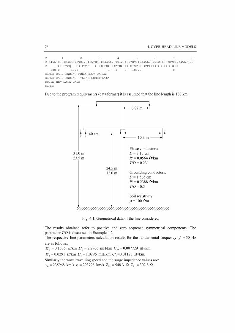
76 4. OVER-HEAD LINE MODELS
C 1 2 3 4 5 6 7 8 C 345678901234567890123456789012345678901234567890123456789012345678901234567890 C >< Freq >< FCar > <ICPR> <IZPR> =< DIST > <PP>==< >< >< ><><> 100.0 50.0 1 1 0 180.0 0 BLANK CARD ENDING FREQUENCY CARDS BLANK CARD ENDING "LINE CONSTANTS" BEGIN NEW DATA CASE BLANK
Due to the program requirements (data format) it is assumed that the line length is 180 km.
24.5 m12.0 m
31.0 m23.5 m
6.87 m
10.3 m40 cm
Phase conductors:D = 3.15 cmR' = 0.0564 /kmT/D = 0.231
Grounding conductors:D = 1.565 cmR' = 0.2388 /kmT/D = 0.5
Soil resistivity:= 100 m
Fig. 4.1. Geometrical data of the line considered
The results obtained refer to positive and zero sequence symmetrical components. The parameter T/D is discussed in Example 4.2. The respective line parameters calculation results for the fundamental frequency 501 =f Hz are as follows:
1576.00 =R' Ω/km 2966.20 =L' mH/km 772900.00 =C' μF/km 0291.01 =R' Ω/km 1.0296=1L' mH/km 1C' =0.01123 μF/km.
Similarly the wave travelling speed and the surge impedance values are: 235968=0v km/s 293798=1v km/s 548.3=cZ0 Ω 8.021 3=cZ Ω.

4.1. Single Line 77
Parameters for zero and positive symmetrical components differ since the physical parameters of the earthing conductor and phase conductors are different. The transverse line conductivity G' is usually neglected in such calculations.
4.1.2. Frequency-dependent Model
The frequency dependence of the conductor electric parameters is the result of the skin effect which is caused by pushing of the electromagnetic field outside the conductor when the frequency of the current grows. As a result the effective current conducting cross-section of the wire decreases and the wire resistance grows. Decreasing current reduces the magnetic flux ψ around the conductor thus decreasing the conductor inductance L ( iL /ψ= ) [24].
The frequency dependant parameters depend upon many factors and the most important of them are: the distance between phase and earth conductors and the applied model of the earth which is also the current conductor. The phase conductors in the overhead line can be bundled thus comprising of many wires in various geometrical arrangements being spaced by few tens of centimetres. Also the models of the earth used in calculations may differ significantly since the earth is non-homogenous conducting environment. Thus the calculation of frequency dependent parameters becomes a complex task.
The next example shows how the input data are prepared for subroutine of frequency dependent parameters calculation which is available in ATP–EMTP.
Example 4.2. Determine the frequency dependent parameters of 400 kV line from Example 4.1. Coefficient DT/ (Thickness/Diameter) is necessary for calculation of the skin effect (Fig. 4.1) since the conductor is represented by a pipe of external diameter D and thickness T. For the homogenous wire T/D = 0.5.
Again the LINE CONSTANTS procedure is used and the input data are arranged as follows: BEGIN NEW DATA CASE C Line 400 kV C LINE CONSTANTS METRIC FREQUENCY C Data for LINE CONSTANTS C 345678901234567890123456789012345678901234567890123456789012345678901234567890 1 .231 .0564 4 3.15 -10.3 24.5 12.0 40.0 0.0 2 2 .231 .0564 4 3.15 0.0 24.5 12.0 40.0 0.0 2 3 .231 .0564 4 3.15 10.3 24.5 12.0 40.0 0.0 2 0 0.5 .2388 4 1.565 -6.87 31.0 23.5 0 0.5 .2388 4 1.565 6.87 31.0 23.5 BLANK CARD ENDING CONDUCTOR CARDS OF LINE CONSTANTS CASE C 345678901234567890123456789012345678901234567890123456789012345678901234567890

78 4. OVER-HEAD LINE MODELS
100.0 0.1 1 5 5 BLANK CARD ENDING FREQUENCY CARDS BLANK CARD ENDING "LINE CONSTANTS" BEGIN NEW DATA CASE BLANK
The parameters versus frequency characteristics obtained are shown in Fig. 4.2. The plots show that the zero sequence parameters ( 0R' – Fig. 4.2a and 0L' – Fig. 4.2b) change more intensively with frequency than the positive sequence ones ( 1R' – Fig. 4.2a and 1L' – Fig. 4.2b).
L'0m /km
L'1m /km
L'0
L'1
f, Hz0.1 1 10 100 10001.52.02.53.03.54.04.55.0
0.30.40.50.60.70.80.91.0
b)R'/km
R'0 R'1
f, Hz0.1 1 10 100 1000
a)
0.01
0.1
1.0
Fig. 4.2. Frequency characteristics of the 400 kV line: a) resistance and b) inductance
The difference can be attributed to the fact that the skin effect in return (earthing) wire which is of much greater diameter than the phase wires is much more effective. The transverse parameters (capacitances and conductances) are practically frequency independent. However for the sake of calculation stability usually the small value of one of those parameters is used for instance G'= 003 μS/km [3].
Application of frequency dependent parameters to the line model setup is not simple since equations (1.75) are functions of time. Thus the frequency dependent model must be based on Fourier transform.
The Fourier transform of (1.75) can be determined by use of the following fundamental relations:
x
xUttxux
tx
txu tt
dj(dde
ddde jj ),),(),(
00
ωωω ==∂
∂∫∫∞
−∞
− (4.1)
)j,(jde),(je),(de),(
0
jj
0
j ωωω ωωω xUttxutxutt
txu ttt =+∂=∂
∂∫∫∞
−∞
∞−
−∞
− (4.2)

4.1. Single Line 79
The function ), ωj(xU is complex. For fixed frequency ), ωj(xU is the voltage phasor as used in steady state analysis of electric networks.
Formulas (4.1) (4.2) can also be applied to the current equations in (1.75). Thus the line equations (1.75) in frequency domain are now:
( )
( ) )j,(jd
)j,(d
)j,(jd
)j,(d
ωωω
ωωω
xUC'G'x
xI
xIL'R'x
xU
+=−
+=−
and using the substitution:
C'G'Y'L'R'Z'
ωωωω
jjjj
+=+=
)()(
(4.3)
finally:
)j,()j(
d)j,(d
)j,()j(d
)j,(d
ωωω
ωωω
xUY'x
xI
xIZ'x
xU
=−
=− (4.4)
The first of the above equations describe the longitudinal line model. Impedance )( ωjZ' is frequency-dependent since )(ωR'R' = and )(ωL'L' = . The second
equation describes the line model for transverse parameters. Usually the components of the admittance )( ωjY' are frequency independent.
The equation (4.4) can also be split into the current and voltage parts. Differentiating the first equation in (4.4) with respect to x and applying the result to the second one we get:
),()()(),2 ωωωω jjj
dj(d2
xUY'Z'xxU = (4.5)
Using notation )()(2 ωωγ jj Y'Z'= the final form of (4.5) is:
),(), 22 ωγω j
dj(d2
xUxxU = (4.6)
The general solution of (4.6) is as below [77]:
)sinh()cosh()j,( 11 xBxAxU γγω += (4.7)
where: 1A 1B – constants calculated from boundary conditions and

80 4. OVER-HEAD LINE MODELS
βαωωγ jjj +== )()( Z'Y' (4.8)
Out of the two the square root values only the one for which 0≥α is valid. The parameter γ [1/km] is known as the line propagation velocity constant; α is the line attenuation constant (Np/km)1 and β is the phase propagation constant (rad/km).
Substituting (4.7) into the second equation in (4.4) we get:
( ))cosh()sinh(1)j,( 11 xBxAZ
xIf
γγω +−= (4.9)
where: γ
ωωωω )(
)()()( j
jjj Z'
Y'Z'ZZ ff === (4.10)
is the complex surge impedance of the line. Constants 1A 1B can be determined from the boundary conditions: at beginning of
the line 0=x (subscript 1) and at the end lx = (subscript 2) and in such case (4.7) (4.9) are as follows:
101101 )sinh()cosh()j,()j( AxBxAxUU xx =+== == γγωω (4.11)
)sinh()cosh()sinh()cosh()j,()j( 11112 lBlAxBxAxUU lxlx γγγγωω +=+== ==
(4.12)
( )f
xf
x ZBxBxA
ZxII 1
01101 )cosh()sinh(1)j,()j( −=+−====
γγωω (4.13)
( )
( ))cosh()sinh(1
)cosh()sinh(1)j,()j(
11
112
lBlAZ
xBxAZ
xII
f
lxf
lx
γγ
γγωω
+−=
+−== ==
(4.14)
Assuming that the voltage and current at the end of the line are known and )j(1 ωU )j(1 ωI are to be determined then the respective solution, for the line output currents
flowing in directions as shown in Fig. 4.3, is:
⎥⎦
⎤⎢⎣
⎡−
⎥⎥⎥
⎦
⎤
⎢⎢⎢
⎣
⎡=⎥
⎦
⎤⎢⎣
⎡)j()j(
)cosh()sinh()j(
1)sinh()j()cosh(
)j()j(
2
2
1
1
ωω
γγω
γωγ
ωω
IU
llZ
lZl
IU
f
f
(4.15)
1 Np (neper) is the unit of attenuation.1 Np = 8.686 dB.
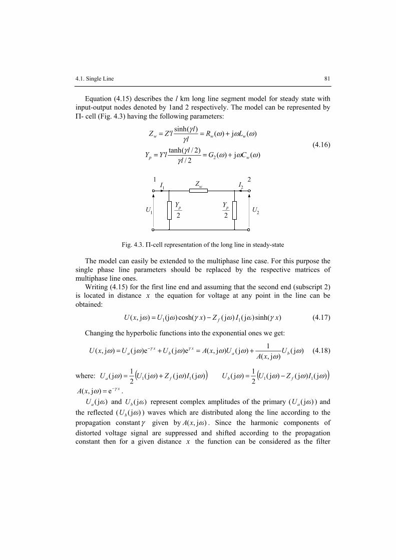
4.1. Single Line 81
Equation (4.15) describes the l km long line segment model for steady state with input-output nodes denoted by 1and 2 respectively. The model can be represented by Π- cell (Fig. 4.3) having the following parameters:
)(j)(
2/)2/(tanh
)(j)()(sinh
2 ωωωγ
γ
ωωωγ
γ
wp
www
CGl
lY'lY
LRl
lZ'lZ
+==
+== (4.16)
Zw
U1 U2
I1
1I2
2
2pY
2pY
Fig. 4.3. Π-cell representation of the long line in steady-state
The model can easily be extended to the multiphase line case. For this purpose the single phase line parameters should be replaced by the respective matrices of multiphase line ones.
Writing (4.15) for the first line end and assuming that the second end (subscript 2) is located in distance x the equation for voltage at any point in the line can be obtained:
)sinh()j()j()cosh()(j)j,( 11 xIZxUxU f γωωγωω −= (4.17)
Changing the hyperbolic functions into the exponential ones we get:
)(),(
1)(),()()(),( ωω
ωωωωω γγ jj
jjejejj bax
bx
a UxA
UxAUUxU +=+= − (4.18)
where: ( ))()()(21)( 11 ωωωω jjjj IZUU fa += ( ))()()(
21)( 11 ωωωω jjjj IZUU fb −=
xxA γω −= ej ),( . )( ωjaU and )( ωjbU represent complex amplitudes of the primary ( )j( ωaU ) and
the reflected ( )j( ωbU ) waves which are distributed along the line according to the propagation constantγ given by )j,( ωxA . Since the harmonic components of distorted voltage signal are suppressed and shifted according to the propagation constant then for a given distance x the function can be considered as the filter

82 4. OVER-HEAD LINE MODELS
transmittance of frequency response determined by xxA αω −= e)j,( and the phase response given by ( ) xxA βω je)j,(arg −= . In case of the overall line ( lx = ) we get:
llAA γωω −== ejj ),()( lA αω −= ej )( ( ) lA βω jej −=)(arg (4.19)
The next example explains the discussed line characteristics.
Example 4.3. Analyse the considered frequency characteristics for the 400 kV line from Example 4.1.
The example of imaginary component distribution for wave of frequency 2000=pf Hz in the 300=l km long 400 kV line is shown in Fig. 4.4. Two standing waves for positive and zero
sequence voltage components are presented for comparison. The waveforms correspond to the following functions::
( ))j()j,(Re)( 111 pap UxAxU ωω= ( ))j()j,(Re)( 000 pap UxAxU ωω=
and: )j(1
11e)j,( pppxA βαω +−= )j(
000e)j,( pp
pxA βαω +−= 1)()( 01 == papa UU ωω jj ; subscript p
refers to the selected frequency while respective components are denoted by 0 and 1. The line parameters for frequency 2000=pf Hz (Example 4.1) are given in Table 4.1.
xe 1α−
xe 0α−
Fig. 4.4. Distribution of the wave along the line
Table 4.1. 400 kV line parameters for frequency 2 kHz
Parameter Positive sequence component Zero sequence component R' Ω/km 0.09619 2.0075
L' mH/km 1.0194 1.968 C' μF 0.01123 0.00779
α Np/km 1.596⋅10–4 0.0020 β rad/km 0.0425 0.0491

4.1. Single Line 83
The wavelength can be determined by examination of arguments of functions )j,(1 pxA ω
and ),(0 pxA ωj . The resulting general relation is: β
λ π2= , which for the considered example
yields: 097.1280 =λ km and 776.1471 =λ km. According to the known relation the wave propagation velocity is:
βωλ == fv and: 5
0 10562.2 ⋅=v km/s 51 10955.2 ⋅=v km/s.
The wave propagation velocity depends mainly on the line parameters. The attenuation of the phase-phase loop is much lower than for phase –earth one (zero sequence component).
Multiplying the current equation in (4.15) by fZ and subtracting it from the first (voltage) one we get:
( ) lff IZUIZU γωωωωωω −+=− e)j()j()j()j()j()j( 2211 (4.20)
or in alternative voltage and current notations:
( ) )j()j()j()j()j()j()j( 2211 ωωωωωωω AIZUIZU ff ++= (4.21)
( ) )j()j()j(/)j()j(/)j()j( 2211 ωωωωωωω AIZUZUI ff +−= (4.22)
where: A(jω) is like in (4.19). If (4.20) is applied to the lossless line with frequency independent parameters then
we have:
C'L'ZZ ff /)( ==ωj L'C'ωγ j= ωτγ jee −− =l
After inverse Fourier transformation of (4.20) we get:
)()()()( 2211 ττ −+−=− tiZtutiZtu ff
and: ωτωτ je)j()( −=− XtxF . being is the same as (1.83) which describes the lossless line in time domain. Thus (4.21) can be considered as an operator equation in the line model. Parameters Zf (jω) and A(jω) are now the filter transmittances revealing the respective frequency responses. The complex propagation function A(jω) can be deemed as a product of lumped parameter transmittance P(jω) and the delay line so that:
fPA ωτωω je)j()j( −= (4.23)
where: fτ is the propagation time of the fastest wave component. The delay fτ can be determined from the equation:

84 4. OVER-HEAD LINE MODELS
( ) ( ) ( ) lPAPf βωωωωτ +=−= )(arg)(arg)(arg jjj (4.24)
and P(jω) comes from (4.19) and (4.23):
lAP αωω −== e)j()j( (4.25)
The filters based on the above equations represent the frequency dependent line model with parameters expressed by functions Zf (jω) and A(jω) in (4.21) (4.22). The frequency properties of those functions are illustrated by the following example.
Example 4.4. Examine the frequency characteristics of positive and zero sequence components for 400 kV line discussed in Example 4.1. Assume that the line is 180 km long.
Like in Example 4.1 calculations have been carried out by use of the LINE CONSTANTS auxiliary program in ATP–EMTP for the frequency range 0.001 Hz–1 MHz. The frequency response of the propagation function A(jω) is shown in Fig. 4.5. The continuous line (1) denotes the positive sequence component and the dotted line (2) – refers to the zero sequence one. The phase displacement of the function ( ) βω lA −=)j(arg is nearly linear since v/ωβ = and the propagation velocity v is practically constant in the considered frequency range so the coefficient βl (the total phase displacement between the line input and output) is proportional to the wave length.
Fig. 4.5. Frequency characteristic of the propagation function A(jω): a) frequency response b) phase response
For the lossless line there is L'C'v ωωβαγ jjj ==+= / that implies L'C'A ωω jej −=)( and the function A(jω) represents the signal distortion caused by the frequency dependent line parameters. The phase characteristic comprises of two parts. The first part is related to the phase response of the filter and the second one reflects the phase displacement fωτ caused by wave propagation time (delay) (4.23).

4.1. Single Line 85
The propagation time fτ should have the least value which corresponds to the highest frequency in the considered frequency range [58]. The phase response =)j(arg ωP lf βωτ − of the function P(jω) for positive sequence (curve 1) and zero sequence (2) component of the line considered are shown in Fig. 4.6.
– /2
0
10–2 100 102 104 f, Hz
1
2arg(
P(j
)), r
ad
Fig. 4.6. Phase response of P(jω) for 400 kV line: 1 – positive sequence component 2 – zero sequence component
The values of propagation time τf for both components have been estimated for the frequency fgr for which = )( ωjP drops below 0.01 (Fig. 4.5a) according to the relation: ( ) ==
= grfff vl /τ
( )grff
l=
ωβ / . The respective frequency response of wave impedance is shown in Fig. 4.7. Thus
the equivalent wave impedance can be considered as the lumped element of adequate frequency response.
200300400500600700800900
10–2 100 102 104 f, Hz 10–2 100 102 104 f, Hz
0
|Zf(j
ω)|,
Ω
1000
arg(
Z f(jω)
), °
a) b)
2
1
2
1
–30
–25
–20
–15
–10
–5
Fig. 4.7. Frequency characteristics of the line surge impedance a) frequency response b) phase characteristic; 1 – for positive sequence 2 – for zero sequence

86 4. OVER-HEAD LINE MODELS
The respective filter transmittances in Laplace sense corresponding to line parameters Zf(s)
sfZ=
=ω
ωj
j )( ands
PsP=
= ωωj
j )()( can be determined by rules of
minimum-phase system design known from the control system theory [21, 24] if the frequency response )( ωjfZ and )( ωjP are known (they can be determined as in
Example 4.1). If the transmittance considered can be expressed in the factor form which, for instance, in case of wave impedance is:
))..()(())..()((
..
..)()()(
21
211
10
110
m
n
m
mm
n
nn
k
kZ
kkk
kkk
f bsbsbszszszs
kbsbsbasasa
sMsLsZ
−−−−−−
=++++++
== −
−
(4.26)
then zeroes and poles of such a transmittance can be determined by use of the Bode plot (logarithmic) method [58].
Then the transmittance can be implemented by chain of parallel RC cells. The conditions of such implementation is that poles and zeros alternate on the real axis of the s plane and one pole is located closest to the origin as it is shown in Example 4.5.
Example 4.5. Design the chain of parallel RC cells which approximate the wave impedance of 400 kV line for zero sequence component Zf0(jω). The line parameters are as in Example 4.1.
The frequency response of the wave impedance considered is shown in Fig. 4.7 plot 2. The following transmittance is obtained (calculated in MATLAB) [66] for the fifth order approximation:
))()()()(())()()()(()(
54321
543210 bsbsbsbsbs
zszszszszsksZ Zf −−−−−−−−−−=
where: 15.446=Zk 37112 −=1z 1266.4 −=2z 18.708 −=3z 4.469 −=4z 088.15 −=z
33789 −=1b 1165.5 −=2b 14.013 −=3b 3.929 −=4b 0.9057 −=5b . The implementation requirements are met so after partial fraction decomposition of )(0 sZ f we get:
5
5
4
4
3
3
2
2
1
10 )(
bsK
bsK
bsK
bsK
bsKksZ Zf −
+−
+−
+−
+−
+= where: ibsifi bssZK
=−= ))((0 .
and also: 6
1 10478.1 ⋅=K 42 10935.4 ⋅=K 2.23353 =K 0.3964 =K 86.1555 =K .
Now using the Foster’s method the required RC circuit is obtained (Fig. 4.8) for which the respective parameters are [66]:
ZkR =0 iii bKR /−= ii KC /1= i = 1 ... 5. After relevant substitution we get: R0 = 44615 Ω R1 = 43738 Ω R2 = 42345 Ω R3 = 16665 Ω R4 = 10078 Ω R5 =17210 Ω C1 = 06766 μF C2 = 2026 μF C3 = 4282 μF C4 = 2525 μF C5 = 6416 μF.

4.1. Single Line 87
R0
R1
C1
R2
C2
R3
C3
R4
C4
R5
C5
Fig. 4.8. The RC chain representing transmittance )(0 ωjfZ
Comparison of wave impedance frequency response obtained from calculations and from the RC model is shown in Fig. 4.9.
|Zf0
(jω)|,
Ω
10–2 100 102 104 f, Hz
1
2
arg(
Z f0(jω
)), °
10–2 100 102 104 f, Hz
1
2
a) b)
400
500
600
700800
9001000
–12
–10
–8
–6
–4
–2
0
Fig. 4.9. Frequency response of zero sequence wave impedance Zf0 (jω): a) magnitude; b) phase 1 – calculations 2 – frequency response of the RC model
The numerical model of the equivalent RC circuit can be derived using the model setup rules for lumped element circuit. A single i-th RC cell in the chain is described by the following continuous differential equation:
)(1)(1)( tiC
tuCRt
tufZ
ii
ii
i +−=d
d (4.27)
and the known solution of the equation is:
ττταα dee ∫ −−−− +=t
tZ
t
ii
tti f
iiii iC
tutu0
0 )(1)()( )(0
)( (4.28)
where: iii CR/1=α 0t denotes calculation starting time. Using the trapezoidal integration method we get ( Ttt =− 0 – calculation step):
( ))()1(e2
)1(e)( kikiCTkuku
ff
iiiiZZ
T
ii
Ti +−+−= −− αα

88 4. OVER-HEAD LINE MODELS
and after rearrangement: )1()()( −+= kvkiRku iZeii f
(4.29)
where: 22
i
iei
TKCTR == ( ))1()1(e)( −+−=− − kiRkuikv
f
iZeii
Ti
α .
Series connection of m RC cells along with resistance R0 results in the following numerical model:
)1()()( −+= kvkiRkufff ZZZ (4.30)
where: ∑=
+=m
f
k
ieiZ RRR
10 ( )∑
=
− −+−=−m
f
i
f
k
iZeii
TZ kiRkukv
1
)1()1(e)1( α .
Writing (4.30) in alternative current form we get: )1()()( −+= kjkuGki
ff ZfZ (4.31)
where: fZf RG /1= )1()1( −−=− kvGkj
ff ZfZ .
In case of propagation function A(jω) the model can be applied to approximation of P(jω) (4.23) as it is illustrated by the following example.
Example 4.6. Design the numerical model of function P0(jω) (zero sequence component) for 400 kV line considered in Example 4.4.
The frequency response of P0(jω) is shown in Fig. 4.5a plot 2. Again applying the fifth order approximation we get:
))()()()(())()()(()(
54321
43210 bsbsbsbsbs
zszszszsksP P −−−−−−−−−=
where: 0465.0=Pk 29424 −=1z 659.99 −=2z 12.89 −=3z 0.1915 −=4z 9842.8 −=1b 3089.5 −=2b 4.5693 −=b 12.58 −=4b 0.1908 −=5b . Partial fraction decomposition leads to the equation:
5
5
4
4
3
3
2
2
1
10 )(
bsK
bsK
bsK
bsK
bsKksP P −
+−
+−
+−
+−
+=
where: ibsii bssPK
=−= ))((0 ,
and: 6.23721 −=K 3.31062 =K 41.923 =K 2916.04 =K 4
5 100.6 −⋅=K . The approximation of the logarithmic frequency response used [34] yields the negative 1K so the in RC circuit model cannot be applied. However calculations can be carried out according to (4.27)–(4.30) for ii b−=α . (4.31) can be written in changed form for the current excitation
)(kiPw (the input current):

4.1. Single Line 89
)1()()( −+= kjkiki PPwP
where: ∑=
−=−=−5
1
)1()1()1(i
PiPPP kikvGkj and by analogy to (4.30):
∑=
+= 5
1
2
2
iiP
P
KTkG ∑
=
− ⎟⎠
⎞⎜⎝
⎛ −+−=−5
1
)1(2
)1()1(i
Pwi
iT
P kiTKkuekv iα .
After simplification the equation for the current )(kiPi is: )1()()( −+= kjkiLki PiPwiPi i = 1 ... 5
where: )1()1()1()1( −−+−=− kikLkiekj PwiPiTb
Pii iPi KGTL
2= .
Comparison of respective frequency responses is shown in Fig. 4.10.
Relatively big difference in phase characteristics (Fig. 4.10b) can be attributed to large error in estimation of the original characteristic for high frequency. If )(sP is the correct representation of P(jω) then fτ can be determined from (4.24). Referring calculations to the fundamental frequency ω1 and using (4.8) we get:
( ) ( )( ))()(arg)(arg1111
1
ωωωω
τ jjj Y'Z'lPf += (4.32)
arg(
P 0(j
)), r
ad
|P0(j
)|
Fig. 4.10. Frequency response of zero sequence surge impedance P0 (jω)): a) magnitude; b) phase 1 – calculations 2 – frequency response of the fifth order model
Both functions Zf (jω) and A(jω) can now be represented by the equivalent lumped parameter circuits described by the respective transmittances )(sZ f )(sP and time delay fτ . The equation (4.22) takes the following form in time domain:
)()()( 111 mkjkikifZ −+= (4.33)

90 4. OVER-HEAD LINE MODELS
where: fZi1 corresponds to (4.31) for node 1; )(1 mkj − is the current 'seen' from the
other end of the line; m is the discrete time delay calculated from fτ . Taking into account (4.31) the value of excitation in node 2 of the line is given by
the following sum of currents:
)1()()()()()( 222222 −++=+= kjkikuGkikikiff ZfZPw (4.34)
Introducing the delay m and including )(sP we get (see Example4.6):
)1()()( 221 −−+−=− mkjmkimkj PPw (4.35)
where: ∑=
−−=−−mk
iPiP mkimkj
122 )1()1(
)1()()( 222 −+= kjkiLki PiPwiPi mki ..,,1=
)1()1(e)1( 222 −+−=− kiLkikj PwiPiTb
Pii iPi KGTL
2=
∑=
+=
mk
iiP
P
KTkG
1
2
2 .
mk denotes the number of poles ib in )(sP while Pk and iK come from the partial fraction decomposition.
Relations (4.31)–(4.35) describe the digital model of the line with frequency dependent parameters. (Fig. 4.11).
The currents )(1 mkj − )(2 mkj − ‘seen’ from the other side of the line should be calculated from (4.34) (4.35).
u1(k)
1 i1(k)
Gf
j1(k–m)
i1Z (k)f
j1Z (k–1)f
u2(k)
2i2(k)
Gf
j2(k–m)
i2Z (k)f
j2Z (k–1)f
Fig. 4.11. The equivalent circuit of the line with frequency dependent parameters.
The currents )1(1 −kjfZ )1(2 −kj
fZ along with the conductance fG represent the
wave impedance Zf (jω) according to (4.31).

4.2. Multi-phase Line Model 91
4.2. Multi-phase Line Model
4.2.1. Lumped Parameter Model
The generalized model of multi-phase line was developed by Carson [14]. In the model the multi-conductor arrangement of phase wires along with equivalent arrangement of identical and symmetrical with respect to earth surface return wires (Fig. 4.12) is considered.
Parameters of the equivalent line circuit can be determined under assumption that the sum of currents in all conductors (Fig. 4.122 ) is equal to zero. The equivalent circuit of the considered line segment is shown in Fig. 4.13. Vector of voltage drop across that segment is given by the following equation:
( )
⎥⎥⎥⎥⎥⎥⎥⎥⎥
⎦
⎤
⎢⎢⎢⎢⎢⎢⎢⎢⎢
⎣
⎡
+=
⎥⎥⎥⎥⎥⎥⎥⎥⎥
⎦
⎤
⎢⎢⎢⎢⎢⎢⎢⎢⎢
⎣
⎡
ΔΔΔ
NM
N
N
C
B
A
C
B
A
I
IIIII
UUU
MM
2
1
0
00 LR ωj (4.36)
where:
⎥⎥⎥⎥⎥⎥⎥⎥
⎦
⎤
⎢⎢⎢⎢⎢⎢⎢⎢
⎣
⎡
+
++
++
=
DNMDDDD
DDNDDD
DDDCDD
DDDDBD
DDDDDA
RRRRRR
RRRRRRRRRRRRRRRRRRRRRRRR
L
MMMMMM
L
L
L
L
1
R kmL=L
AR ... NMR – conductor resistances (in general temperature, frequency and current dependent)
lfRD ⋅×= −710869.9 (Ω) f – frequency (Hz) l – conductor length (m);
km
kmkm d
DlL ln2
0
πμ= (H) 7
0 104 −×= πμ H/m – magnetic permeability mk , – conductor
numbers kkd – conductor radius (equivalent for bunch wires).

92 4. OVER-HEAD LINE MODELS
dkm
k
m
k'
m'
Dkm
Fig.. 4.12. Conductor arrangement for equivalent overhead line
In analysis of three-phase lines the simplified line model is applied in which M return conductors is replaced by one equivalent wire.
Fig 4.13. The equivalent circuit of the multiphase line
In more detailed notation (4.36) takes the form:

4.2. Multi-phase Line Model 93
⎥⎥⎥⎥⎥⎥⎥⎥
⎦
⎤
⎢⎢⎢⎢⎢⎢⎢⎢
⎣
⎡
⎥⎥⎥⎥⎥⎥⎥⎥
⎦
⎤
⎢⎢⎢⎢⎢⎢⎢⎢
⎣
⎡
=
⎥⎥⎥⎥⎥⎥⎥⎥
⎦
⎤
⎢⎢⎢⎢⎢⎢⎢⎢
⎣
⎡
ΔΔΔ
+++++
+
+
+
+
NM
N
C
B
A
MMMMMM
M
M
M
M
C
B
A
I
IIII
ZZZZZ
ZZZZZZZZZZZZZZZZZZZZ
UUU
M
L
MMMMMM
L
L
L
L
M
1
)3(4)3(3)3(2)3(1)3(
)3(444434241
)3(334333231
)3(224232221
)3(114131211
0
0 (4.37)
where: kkDkkk LRRZ ωj++= kmDkm LRZ ωj+= .
The equation (4.37) can be written in compact form as:
⎥⎦
⎤⎢⎣
⎡⎥⎦
⎤⎢⎣
⎡=⎥
⎦
⎤⎢⎣
⎡
N
f
DC
BA
II
ZZZZ
0ΔU
(4.38)
Basing on (4.38) the following equations can be written:
NDfC
NBfA
IZIZ0
IZIZΔU
+=
+= (4.39)
The second equation yields: fCDN IZZI 1−−= (4.40)
Substituting (4.40) to the first equation in (4.39) we get:
ff IZΔU = (4.41)
where:
⎥⎥⎥
⎦
⎤
⎢⎢⎢
⎣
⎡=−= −
CCBCAC
BCBBAB
ACABAA
CDBAf
ZZZZZZZZZ
ZZZZZ 1 (4.42)
is the parameter matrix of the equivalent three-phase line (Fig. 4.14). The following relations are valid for transposed line in frequency domain:
SCCBBAA ZZZZ === MBCACAB ZZZZ === .

94 4. OVER-HEAD LINE MODELS
Fig. 4.14. Simplified circuit of three-phase line
In time domain voltage drop across the considered line segment is given by:
)()()( tt
tt ffff ILIRΔUdd+= (4.43)
where:
⎥⎥⎥
⎦
⎤
⎢⎢⎢
⎣
⎡
−−−
=)()()()()()(
)(
21
21
21
tutututututu
t
CC
CB
AA
ΔU ⎥⎥⎥
⎦
⎤
⎢⎢⎢
⎣
⎡=
)()()(
)(tititi
t
C
B
A
fI
⎥⎥⎥
⎦
⎤
⎢⎢⎢
⎣
⎡=
CCBCAC
BCBBAB
ACABAA
f
RRRRRRRRR
R ⎥⎥⎥
⎦
⎤
⎢⎢⎢
⎣
⎡=
CCBCAC
BCBBAB
ACABAA
f
LLLLLLLLL
L .
Using the generalized line model (Fig 4.12) the equivalent transverse line model can be derived under general assumption that all conductors are isolated one from each other entirely. The electric charges q in physical conductors and in the equivalent ones located under the earth (mirror reflection) are equal and opposite so it can be assumed that the voltage between k-th conductor and the earth surface is equal to the half of the voltage between the conductor and its mirror reflection under the earth [36]. If so then:
km
kmM
iikmkN d
DqUU ln2
121 3
10∑+
=
==επ
(4.44)
where: 122
00 10854.81 −×==
cμε F/m – electric permeability, iq – charge in i-th
conductor (C/m), c – light velocity (m/s).

4.2. Multi-phase Line Model 95
Similar equations can be written for each isolated phase conductor while the other conductors are earthed and connected to the zero reference potential. Using the matrix-vector notation the equations take the form:
⎥⎥⎥⎥⎥⎥⎥⎥
⎦
⎤
⎢⎢⎢⎢⎢⎢⎢⎢
⎣
⎡
⎥⎥⎥⎥⎥⎥⎥⎥
⎦
⎤
⎢⎢⎢⎢⎢⎢⎢⎢
⎣
⎡
=
⎥⎥⎥⎥⎥⎥⎥⎥
⎦
⎤
⎢⎢⎢⎢⎢⎢⎢⎢
⎣
⎡
+++++
+
+
+
+
NM
N
C
B
A
MMMMMM
M
M
M
M
C
B
A
q
qqqq
PPPPP
PPPPPPPPPPPPPPPPPPPP
UUU
M
L
MMMMMM
L
L
L
L
M
1
)3(4)3(3)3(2)3(1)3(
)3(444434241
)3(334333231
)3(224232221
)3(114131211
0
0 (4.45)
where:
km
kmkm d
DP ln2
1
0επ= (m/F) (4.46)
kmP is known as Maxwell coefficient. Similarly to (4.37) the equation (4.45) can be simplified and:
⎥⎦
⎤⎢⎣
⎡⎥⎦
⎤⎢⎣
⎡=⎥
⎦
⎤⎢⎣
⎡
N
f
DC
BAf
PPPP
0U
(4.47)
from which:
( ) fCDBAf qPPPPU 1−−= (4.48)
or alternatively
( ) fffCDBAf UCUPPPPq =−=−− 11 (4.49)
where:
( )⎥⎥⎥
⎦
⎤
⎢⎢⎢
⎣
⎡=−=
−−
CCBCAC
BCBBAB
ACABAA
CDBAf
CCCCCCCCC
11PPPPC (F/m) (4.50)
is the capacitance matrix of the equivalent three-phase system. Conductance is an active element of the transverse line model. Confining
considerations to linear case the corresponding model will be described by the following equation:

96 4. OVER-HEAD LINE MODELS
ffG UGI = , ⎥⎥⎥
⎦
⎤
⎢⎢⎢
⎣
⎡=
CCBCAC
BCBBAB
ACABAA
f
GGGGGGGGG
G (S/m) (4.51)
In power line models conductance is not taken into account as being negligibly small with respect to line susceptance. Thus the line model looks like it is shown in Fig. 4.15.
RA LAiA1
RB LBiB1
RC LCiC1
LAB
LAC LBC
C11 –CAC–CAB
–CBC
C33
C22
C11–CAC–CAB
–CBC
C33
C22
iA2
iB2
iC2
A1
B1
C1
A2
B2
C2
Fig. 4.15. The equivalent circuit of the three-phase line
The current flowing through the transverse elements at any side of the three-phase line model can be determined by the following equation:
ffY UYI = , fff CGY ωj+= (S/m) (4.52)
in frequency domain or by:
)()()( tt
tt ffffY UCUGIdd+= (4.53)
in time domain. It should be noted that the respective capacitances in the line model are divided
into two equal parts connected to each end of the line. The values of phase-to-phase capacitances are negative while the respective phase-to- ground capacitance values are:
.,,
33
22
11
BCACCC
BCABBB
ACABAA
CCCCCCCCCCCC
−−=−−=−−=
and if the line is transposed then:

4.2. Multi-phase Line Model 97
SCCBBAA CCCC === MBCACAB CCCC === .
In the model of transposed line the parameters in all phases can be assumed as being equal and then the line parameters for symmetrical components can be used. The respective relations can be obtained after transformation of phase coordinates into the symmetrical ones by use of the fundamental formula:
sf SUU = (4.54)
for voltages (the same formula holds for currents) where:
⎥⎥⎥
⎦
⎤
⎢⎢⎢
⎣
⎡=
aaaa
2
2
11
111
31S
23
213/2 jea πj +−== (4.55)
⎥⎥⎥
⎦
⎤
⎢⎢⎢
⎣
⎡=
2
1
0
UUU
sU – symmetrical voltage(current) component vector.
Applying transformation (4.54) to (4.41) the relation between phase fZ and
symmetrical sZ component impedance matrices is obtained and:
SZSZ fs1−= (4.56)
If the three-phase system is transposed then the matrix of symmetrical impedance components is diagonal:
⎥⎥⎥
⎦
⎤
⎢⎢⎢
⎣
⎡=
2
1
0
ZZ
Z
sZ (4.57)
In case of power line: 21 ZZ = , and (4.56) shows that for the transposed line the following relations hold:
MS ZZZ 20 += MS ZZZ −=1
32 10 ZZZ S
+= 3
10 ZZZ M−= .
It should be born in mind that transformation into symmetrical components refers to complex vectors of currents and voltages which represent fixed frequency harmonic functions of time in steady state. Therefore the transformation is not applied directly to transient analysis of electric networks. However all the relations shown are important

98 4. OVER-HEAD LINE MODELS
for the model setup since line and cable parameters are very frequently available in symmetrical component form.
4.2.2. Distributed Parameters Model
Derivations of the multi-phase distributed parameter line model and of the single phase one are very much alike. In case of n phases (1.75) takes the form:
ttx'tx'
xtx
ttx'tx'
xtx
∂∂+=
∂∂−
∂∂+=
∂∂−
),(),(),(
),(),(),(
UCUGI
ILIRU
(4.58)
where:
⎥⎥⎥⎥
⎦
⎤
⎢⎢⎢⎢
⎣
⎡
=
),(
),(),(
),( 2
1
txu
txutxu
tx
n
MU
⎥⎥⎥⎥
⎦
⎤
⎢⎢⎢⎢
⎣
⎡
=
),(
),(),(
),( 2
1
txi
txitxi
tx
n
MI – voltages and currents of n-phase line;
⎥⎥⎥⎥
⎦
⎤
⎢⎢⎢⎢
⎣
⎡
=
nnnn
n
n
R'R'R'
R'R'R'R'R'R'
'
L
MLMM
L
L
21
22212
11211
R (Ω/km) – matrix of ‘per unit’ line resistance (similarly to
'G 'L 'C ). In general, parameters in (4.58) are frequency dependent but for the sake of model
simplicity this effect can be neglected.
a) Constant Parameters Model
In case of lossless multiphase line (4.58) can be written as (by analogy to (1.79)):
0
0
2
2
2
2
2
2
2
2
=∂∂−
∂∂
=∂∂−
∂∂
t''
x
t''
xILCI
UCLU
(4.59)
The matrices:
''u CLA = ''i LCA =
are complete and symmetrical. Therefore:
( )Tui AA = (4.60)

4.2. Multi-phase Line Model 99
Subscripts i and u indicate either current or voltage matrix in (4.59). The line model will be simplified significantly if the matrices in (4.59) are diagonal
since in such case the multiphase system gets uncoupled and the model of n-phase line splits into n single phase ones.
Diagonalization of matrix iA is described by the equation:
iiii TATA 1mod
−= (4.61)
where: iT is the square eigenvalue matrix in which the k-th column ks (the eigenvector2 of iA ) is the function of k-th eigenvalue kλ of the matrix iA so that the following equation is satisfied [21]:
( ) 0=− kki s1A λ (4.62)
Relation (4.61) is known as similarity transformation in which the eigenvalues of iA and modiA are the same. For the voltage equation in (4.59) we get similarly:
uuuu TATA 1mod
−= (4.63)
The respective inverse transformations yield:
1mod
1mod
−
−
==
==
iiii
uuuu
''
''
TATLCA
TATCLA (4.64)
Substitution of (4.64) to (4.59) results in multiphase line equation for modal components:
0
0
2mod
2
mod2mod
2
2mod
2
mod2mod
2
=∂
∂−∂
∂
=∂
∂−∂
∂
tx
tx
i
u
IAI
UAU
(4.65)
where: fii ITITI 11
mod−− == fuu UTUTU 11
mod−− == ;
subscript f indicates phase components. Further, using (4.60) and (4.64) we can write:
( ) ( ) Ti
Ti
Ti
Tiiiuuu TATTATTAT mod
11mod
1mod
−−− == (4.66)
and:
2 Eigenvalues of the square matrix A are equal to the roots of the equation: det(A–λ1) = 0;
Eigenvector x is related to the eigenvalue λ by equation: Ax = λx [21, 83].

100 4. OVER-HEAD LINE MODELS
( ) modmod1
mod11
mod iiuTi
Ti
Tiuu ADADTTATTA === −−− (4.67)
where:
1TTD duT
i == 0≠d (4.68)
is the diagonal matrix of identical elements and modmod iTi AA = .
In many cases it can be assumed that d = 1 and as implication: 1−= uTi TT .
If matrix iA ( uA ) is real (like in (4.59) the eigenvalue matrices iT ( uT ) are also real. Moreover if the parameter matrix is symmetrical then the following relation holds:
1TT =iTi and: T
ii TT =−1 (4.69)
The same applies to matrix Tu. Matrix which satisfies (4.69) is said to be orthogonal3. In such case for d = 1 both matrices are equal:
TTT == ui (4.70)
The condition is also satisfied for transposed lines. If the current and voltage transformation matrices satisfy (4.69) then current and
voltage wave propagation velocities are identical and
⎥⎥⎥⎥⎥⎥⎥⎥
⎦
⎤
⎢⎢⎢⎢⎢⎢⎢⎢
⎣
⎡
==
2
22
21
modmod
1
1
1
n
iu
v
v
v
M
AA (4.71)
kkk C'L'
v 1= – wave propagation velocity for the k-th mode,
kL' kC' – parameters of the k-th mode. Similar relations are valid for wave impedance (1.82).
To include resistance into the line model the line equation in frequency domain can be used (for steady state – see (4.5)):
3 In case of complex form the orthogonal matrix is called the unitary one.

4.2. Multi-phase Line Model 101
0
0
2
2
=−
=−
IZYI
UYZU
''x
''x
dddd
2
2
(4.72)
where: LRZ ωj+=' CGY ωj+=' (conductance G usually neglected),
vectors U and I are function of distance x and by analogy to (4.4):
UYI
IZU
'x
'x
=−
=−
dddd
(4.73)
For complex model (4.72) eigenvalue matrices uT and iT are, generally, also complex and:
iiii
uuuu
TATA
TATA1
mod
1mod
−
−
=
= (4.74)
where: ''u YZA = ''u ZYA = . Using the diagonal matrices of parameters (4.72) takes the form:
0
0
modmod2mod
modmod2mod
=−
=−
IAI
UAU
i
u
x
x
ddd
d
2
2
(4.75)
Interpretation of parameters located in the matrix diagonal is the same as for (4.6):
⎥⎥⎥⎥⎥
⎦
⎤
⎢⎢⎢⎢⎢
⎣
⎡
==
2
22
21
modmod
n
iu
γ
γγ
MAA (4.76)
where: kkkkk Y'Z' βαωωγ jjj +== )()( is the propagation constant for the k-th mode. Comparison of (4.71) and (4.76) yields βk = ω/vk. Substitution of (4.74) to (4.4)
leads to the following relations:
ui
iu
'
'
TYTY
TZTZ1
mod
1mod
−
−
=
= (4.77)

102 4. OVER-HEAD LINE MODELS
The matrices uT and iT in (4.77) are usually complex what makes further calculations cumbersome. To avoid this drawback the matrices are approximated by the respective real ones. This is usually obtained by rotation of the complex matrix to minimize the imaginary parts of complex elements. The respective algorithm of such approximation is shown in [24]: 1. Determine the matrix uuw TT = (the matrix is complex) assuming that the
admittance matrix 'Y comprises of reactance ( imaginary elements) only. 2. Calculate uw
Tuww ' TYTY =mod using (4.77) for 1−= iw
Tuw TT (d = 1 in (4.68)).
3. Since the matrix uwT is complex the real parts appear in elements of modwY . Such elements can be written as: k
kC αω jej mod . To get the normalized (rotated) form of the matrix uwT → uT the columns should be multiplied by the complex
operator 2/kαje . As a result the imaginary elements of the new matrix modY become very small and can be neglected. It must be stressed that the line model in frequency domain (4.72) is meant for
determination of the model parameters and the eigenvalue matrices only while the modelling algorithm remains the same as for the lossless line and can be complemented by the lumped resistance model if necessary (in EMTP the total line resistance is divided into four parts– see Fig. 4.10b). The diagram of the model considered is shown in Fig. 4.16.
The model is realized for each mode according to the algorithm discussed in sect. 1.3.6. The phase vectors of currents and voltages at both sides of the line are transformed into the modal ones in each calculation step. Then after processing by (1.91) and (1.92) the original phase voltages and currents are recovered.
Fig 4.16. Multiphase line in modal arrangement

4.2. Multi-phase Line Model 103
The following example illustrates how the diagonal matrices are calculated in ATP–EMTP.
Example 4.7. Calculate the line parameters of the line in Example 4.1 for phase and modal components assuming that the line is untransposed. Use the LINE CONSTANTS supporting program available in ATP–EMTP.
The line cross section (Fig. 4.1) indicates that the parameters of the middle phase (capacitance and inductance ) (B) differ from the parameters of other phases. The input file for parameter calculating subroutine in ATP–EMTP is also different as compared to the file used in Example 4.1 (the bold typed control line) The control lines read as follows: col. 34: 1 – calculate capacitances for the equivalent three-phase system. col. 38: 1 – calculate impedances for the equivalent system col. 44: 1 – capacitance in (F) units not as ω C (S) – like before; col. 70: 1 – line is untransposed – the current eigenvalue matrix iT .must be calculated BEGIN NEW DATA CASE C Line 400 kV LINE CONSTANTS METRIC C Data for LINE CONSTANTS C 345678901234567890123456789012345678901234567890123456789012345678901234567890 1 .231 .0564 4 3.15 -10.3 24.5 12.0 40.0 0.0 2 2 .231 .0564 4 3.15 0.0 24.5 12.0 40.0 0.0 2 3 .231 .0564 4 3.15 10.3 24.5 12.0 40.0 0.0 2 0 0.5 .2388 4 1.565 -6.87 31.0 23.5 0 0.5 .2388 4 1.565 6.87 31.0 23.5 BLANK CARD ENDING CONDUCTOR CARDS OF "LINE CONSTANTS" CASE C 1 2 3 4 5 6 7 8 C 345678901234567890123456789012345678901234567890123456789012345678901234567890 C >< Freq >< FCar > <ICPR> <IZPR> =< DIST > <PP>==< >< >< ><><> 100.0 50.0 1 1 1 180.0 1 BLANK CARD ENDING FREQUENCY CARDS BLANK CARD ENDING "LINE CONSTANTS" BEGIN NEW DATA CASE BLANK
The relevant fragment of the output file is shown in the next page. Here comes the short comment of results: Capacitance matrix refers to the phase-to- earth capacitances fC (F) (4.50). The lower part of these matrices is given only since the matrix is symmetrical. The same refers to the impedance matrix ff LR ωj+ (Ω). Further the modal parameters are printed: resistance, reactance, wave impedance propagation velocity v : in lossless actual line α (attenuation). All three modal components are of different values. The current eigenvector matrix iT is complex but in this case the normalized imaginary form is given.

104 4. OVER-HEAD LINE MODELS
It can be verified that iT is not orthogonal: 1TT ≠iTi so equation (4.70) does not hold.
Assuming d = 1 calculation of: ( ) 1−= T
iu TT yields:
⎥⎥⎥
⎦
⎤
⎢⎢⎢
⎣
⎡
−−−−−−−−−−−−−
=017084001e3.76012805011865482e7.07106781 011013300e5.80217429014204246e8.48391748 151006496e2.24877083 019739805e5.73790282017084046e3.76012805011865468e7.07106781 011013298e5.80217429
uT .
Let’s follow – using MATLAB - calculation of the eigenvalue matrices uT iT The matrix ''u YZA = is:
⎥⎥⎥
⎦
⎤
⎢⎢⎢
⎣
⎡
−−−−−−−−−−−−−−−−−−−−−−−−−−−
=5j0.0197E + 50.1353E5j0.0085E + 50.0195E5j0.0100E + 50.0205E5j0.0095E +5E 0.02185j0.0192E + 50.1310E5j0.0095E +5E 0.02185j0.0100E + 50.0205E50.0085E j+ 50.0195E5j0.0197E + 50.1353E
'' YZ .
The function eig() calculates eigenvalues and eigenvectors of '' YZ : [TuV]=eig(ZY) where: Tu is the desired matrix uT and V (= V ) is the diagonal eigenvalue matrix:
⎥⎥⎥
⎦
⎤
⎢⎢⎢
⎣
⎡
⋅⋅−⋅⋅−
⋅⋅−=
−−
−−
−−
55
55
55
10j0.0108 + 100.111810j0.0097 + 100.1148
10j0.0383 + 100.1751V .
Columns ks k = 1 2 ... n of the eigenvector matrix [ ]nu sssT L21= are obtained by solution of the following equations (4.62): ( ) 0=− kki s1A λ where: kλ k = 1 2 ... n are the subsequent eigenvalues of '' YZ . MATLAB returns the following result:
⎥⎥⎥
⎦
⎤
⎢⎢⎢
⎣
⎡
−−−−
−−−=
j0.0105 + 0.3754j0.0003 + 0.70710.0179 j 0.5792j0.0280 0.8469j0.0000 + 0.0000j0.0195 0.5727j0.0105 + 0.3754j0.0003 0.70710.0179 j 0.5792
uT .
which is different from that obtained in ATP–EMTP (different sign in the last column). Now the modal admittance matrix modY can be calculated:
5mod 10−⋅
⎥⎥⎥
⎦
⎤
⎢⎢⎢
⎣
⎡
+−++
+==
j0.3769 + 0.0000j0.0000 0.0000j0.0001 + 0.0011j0.0000 0.0000j0.3270 + 0.0000j0.0000 0.00000.0001 j+ 0.0011j0.0000 0.0000j0.2429 + 0.0000
uTu ' TYTY (S/km).
The matrix is not diagonal and not entirely reactive due to the calculation errors and needs to be normalized [24]. Further we skip this stage assuming that the matrix is diagonal and reactive:
⎥⎥⎥
⎦
⎤
⎢⎢⎢
⎣
⎡
⋅⋅
⋅=
−
−
−
5
5
5
10j0.3769 10j0.3270
10j0.2429
modY (S/km).

4.2. Multi-phase Line Model 105 Fr
agm
ent o
f out
put f
ile L
400_
PAR
_PH
.LIS
. … Capacitance matrix, in units of [farads/kmeter ] for the system of equivalent phase conductors.
Rows and columns proceed in the same order as the sorted input.
1 9.962258E-09
2 -1.526980E-09 1.026383E-08
3 -4.467067E-10 -1.526980E-09 9.962258E-09
Impedance matrix, in units of [ohms/kmeter ] for the system of equivalent phase conductors.
Rows and columns proceed in the same order as the sorted input.
1 7.161787E-02
4.594878E-01
2 4.331943E-02 7.258155E-02
1.448813E-01 4.494188E-01
3 4.185105E-02 4.331943E-02 7.161787E-02
1.082764E-01 1.448813E-01 4.594878E-01
Modal parameters at frequency FREQ = 5.00000000E+01 Hz
Mode Resistance Reactance Susceptance The surge impedance in units of [ohms] Lossless and actual Attenuation
ohms/km ohms/km s/km real imag lossless velocity in [km/sec] nepers/km
1 1.570727E-01 7.187872E-01 2.435554E-06 5.464474E+02 -5.900984E+01 5.432519E+02 2.374383E+05 2.360498E+05 1.437217E-04
2 2.976682E-02 3.512114E-01 3.270073E-06 3.280156E+02 -1.387556E+01 3.277220E+02 2.931480E+05 2.928856E+05 4.537410E-05
3 2.846724E-02 2.958356E-01 3.778321E-06 2.801410E+02 -1.344745E+01 2.798181E+02 2.971497E+05 2.968071E+05 5.080878E-05
Eigenvector matrix [Ti] for current transformation: I-phase = [Ti]*I-mode. First the real part, row by row:
5.991431833176021E-01 -7.071067811865462E-01 -4.052167378310909E-01
5.310884029689407E-01 -2.670468863295909E-15 8.195113121629626E-01
5.991431833176025E-01 7.071067811865489E-01 -4.052167378310873E-01
Finally, the imaginary part, row by row:
0.000000000000000E+00 0.000000000000000E+00 0.000000000000000E+00
0.000000000000000E+00 0.000000000000000E+00 0.000000000000000E+00
0.000000000000000E+00 0.000000000000000E+00 0.000000000000000E+00

106 4. OVER-HEAD LINE MODELS
The modal impedance matrix can be calculated using the eigenvalue matrix V and the relation modmodYZV = :
modmod
k
kk Y
Z λ= where subscript k indicates the mode number kλ is the k-th element of the
matrix V. Thus we get:
⎥⎥⎥
⎦
⎤
⎢⎢⎢
⎣
⎡=
j0.2966 + 0.0285 j0.3512 + 0.0298
j0.7206 + 0.1575
modZ (Ω/km).
The modal wave impedance (4.10) is:
mod
modmod
k
kfk Y
ZZ = and further:
⎥⎥⎥
⎦
⎤
⎢⎢⎢
⎣
⎡
−−
−=
j13.48 280.85 j13.88 328.02
j59.16 547.83
modfZ (Ω).
The matrix modfZ elements should be real since they are physical parameters of the actual line. so their imaginary parts can be neglected as coming from the calculation errors. [24]. Now the wave impedance matrix in phase coordinates can be determined using (4.77):
⎥⎥⎥
⎦
⎤
⎢⎢⎢
⎣
⎡== −
387.58 92.5559.5692.55381.5592.5659.5692.56387.58
1mod ifuf TZTZ (Ω)
The eigenvalue matrix T can be calculated using algorithms available in many software packages [66]. The eigenvalue matrices are always real for transposed lines and the relations (4.69) (4.70) hold. Then one of the known from the three-phase circuit theory transformations can be applied for the purpose.
In Clarke transformation4 (also known as 0αβ transformation) the following matrices are applied [19]:
⎥⎥⎥
⎦
⎤
⎢⎢⎢
⎣
⎡
−−−=
312312022
21T
⎥⎥⎥
⎦
⎤
⎢⎢⎢
⎣
⎡
−−−=−
330112111
311T (4.78)
which after normalization to (4.69) yield the following transformation pair:
4 Edith Clarke (1883–1959).

4.2. Multi-phase Line Model 107
⎥⎥⎥⎥⎥⎥⎥
⎦
⎤
⎢⎢⎢⎢⎢⎢⎢
⎣
⎡
−−
−=
23
211
23
211
021
31T
⎥⎥⎥⎥⎥⎥⎥
⎦
⎤
⎢⎢⎢⎢⎢⎢⎢
⎣
⎡
−
−−=−
23
230
21
212
111
311T (4.79)
The parameters of line models derived for (0αβ) modal coordinates and for symmetrical components are the same. If, for instance, matrices (4.79) are used for transformation of transposed line resistance matrix then the result according to (4.77) and (4.69) is:
TTR⎥⎥⎥
⎦
⎤
⎢⎢⎢
⎣
⎡=
⎥⎥⎥
⎦
⎤
⎢⎢⎢
⎣
⎡= −
SMM
MSM
MMS
RRRRRRRRR
RR
R1
1
1
0
0αβ (4.80)
and similarly for the other parameters. Moreover the components αβ are orthogonal in steady state. The αβ coordinates make the base for definition of the space vector [76]:
( )*
2123 fffff
s+=+= βα j (4.81)
which relates the modal coordinates (via (4.79))with the phase ones (ABC):
⎥⎥⎥
⎦
⎤
⎢⎢⎢
⎣
⎡=
⎥⎥⎥
⎦
⎤
⎢⎢⎢
⎣
⎡−
C
B
A
fff
fff
10
T
β
α
and also with the symmetrical components: positive– 1
f i and negative – 2
f ;
superscript * denotes the complex conjugate function. The space vector plays an important role in analysis of three-phase AC circuits [24,
76].
b) Frequency-dependent Line Model
There are many algorithms applied to modelling of multiphase circuits with frequency dependent distributed parameters.
All of them employ of two basic methods of transients representation in the long line:
– calculation of transients by use of the Bergeron’s model (see sect. 1.3.7 that refers to the lossless line),

108 4. OVER-HEAD LINE MODELS
– application of the line model in frequency domain and return to the time domain by use of the inverse Fourier transform.
In case of multiphase line the mutual coupling between particular phases have to be taken into account. To solve this problem one of the following techniques is used: 1. By diagonalization of the multiphase line parameters the line model splits into
many uncoupled single line modal models (the aforementioned approach). 2. The line model is derived for phase coordinates with full parameter matrices under
assumption that the line is untransposed [3 24 58 87]. Below the approach to frequency dependent model of the multiphase line setup as
used in ATP–EMTP is discussed. Application of this approach to a single-phase line is shown sect. 4.1.2.
The multi-phase line model is as shown in Fig. 4.18) and the constant resistances in particular models for modal coordinates are replaced by filters of frequency responses Zf (jω) and A(jω) – like in (4.20) and (4.21) – which are represented by in series connected linear RC cells of transmittances )(sZ f and )(sA respectively.
The models for particular modal components are as shown in Fig. 4.10. The following example shows how the line parameters are calculated.
Example 4.8. Calculate phase and modal parameters of the line in Example 4.1 Assume that the line is untransposed and the line parameters are frequency dependent. Use the JMARTI SETUP procedure available in ATP–EMTP [3].
Model of the frequency dependent long line offered by ATP–EMTP is known as JMARTI [24 58]. The input data for the model are calculated by MARTI SETUP support along with LINE CONSTANTS procedure (Example 4.7) which calculates the basic line parameters. The respective input file is shown below. BEGIN NEW DATA CASE JMARTI SETUP 1.0 Note use of PDT0 = 1 to allow reduction of order $ERASE C Line 400 kV BRANCH PA KA PB KB PC KC LINE CONSTANTS METRIC C Data for LINE CONSTANTS C 345678901234567890123456789012345678901234567890123456789012345678901234567890 1 .231 .0564 4 3.15 -10.3 24.5 12.0 40.0 0.0 2 2 .231 .0564 4 3.15 0.0 24.5 12.0 40.0 0.0 2 3 .231 .0564 4 3.15 10.3 24.5 12.0 40.0 0.0 2 0 0.5 .2388 4 1.565 -6.87 31.0 23.5 0 0.5 .2388 4 1.565 6.87 31.0 23.5 BLANK CARD ENDING CONDUCTOR CARDS OF "LINE CONSTANTS" CASE C 1 2 3 4 5 6 7 8 C 345678901234567890123456789012345678901234567890123456789012345678901234567890 C >< Freq >< FCar > <ICPR> <IZPR> =< DIST > <PP>==< >< >< ><><>

4.2. Multi-phase Line Model 109
100.0 5000.0 180.0 1 1 100.0 50.0 180.0 1 1 100.0 .01 180.0 1 3 4 1 BLANK CARD ENDING FREQUENCY CARDS BLANK CARD ENDING "LINE CONSTANTS" DEFAULT $PUNCH BLANK card ending JMARTI SETUP data cases BEGIN NEW DATA CASE BLANK
The file is very much alike to that in Example 4.7. The notable differences are: – Template JMARTI SETUP indicates the procedure type. – Declaration of nodes for both sides of the line (BRANCH). – Declaration of frequencies (5000, 50 and 0.01 Hz) for which the frequency response is
to be calculated. – The numbers 3 (col. 62) and 4 (col. 65) in the last line. The former indicates that the
frequency response is to be limited to 3 decades on the logarithmic frequency scale and the latter means that the frequency response will be approximated in 4 points within each decade (the numbers should be much greater, say 9, 10; here the small values are used to reduce the output file size).
– Line: $PUNCH means request for the output file *.PCH printout. The output file obtained is as below: -1 PA KA 2. 1.00 -2 3 9 7.3615544019279970000E+02 5.16160970375891200E+03 -4.62836678876982000E+03 2.34908920073601300E+02 2.21428884708777900E+02 4.37807446832278400E+02 3.04928174781558700E+02 2.24591087014093900E+02 4.55263702130293400E+02 1.02771805987124600E+03 2.54324867047940400E-01 2.58267247958202700E-01 4.75266615734256900E-01 7.43821799922729000E-01 1.32805685385736000E+00 1.97949231121861500E+00 2.90622851912841100E+00 6.69971775060332200E+00 1.50030074511141000E+01 1 1.0175027775544130000E-03 4.96285426218186400E+02 4.96823791675659200E+02 -2 PB KB 2. 1.00 -2 3 9 3.4134523824302410000E+02 5.30870510194876300E+02 2.02556181590067800E+01 2.68086180404834000E+02 3.50337060561525300E+02 6.29292421363313800E+02 4.27034282349728200E+02 2.48049348808883800E+03 -1.24353670385984700E+03 3.20930281998335600E+02 1.97752951677736800E-01 2.77134426872770100E-01 5.53515928524456700E-01 1.06867294826728000E+00 2.21360731622174100E+00 3.74655773786376000E+00 8.95197627537033100E+00 9.97585888710791700E+00 1.65795393675722400E+01 1 6.2796878107565830000E-04 4.68508344800458900E+02 4.69023674409433600E+02 -3 PC KC 2. 1.00 -2 3 12 2.9404800772668510000E+02 4.05546694218969000E+02 5.42993557914113500E+01 -1.04056571557813800E+02

110 4. OVER-HEAD LINE MODELS
1.28675981115441400E+02 3.02482667071249200E+02 3.59727123238581600E+02 3.84565069398721800E+02 7.79608344392276500E+02 2.12278761695224800E+03 -1.19401802383945500E+03 1.92613893168671900E+02 2.99694164961513600E+02 1.75763316432903900E-01 2.65010489469351300E-01 2.77287520425178000E-01 2.19898614965812600E-01 5.56134028988414100E-01 1.08558003958717100E+00 2.02757957168211700E+00 4.44555679851210300E+00 9.65825030962793800E+00 1.10764943326363400E+01 1.13569798059043500E+01 1.81281850219694700E+01 1 6.2206229083791410000E-04 4.22175997238486200E+02 4.22644824279796200E+02 0.58407538 -0.70710678 -0.41958805 0.00000000 0.00000000 0.00000000 0.56365939 0.00000000 0.80491722 0.00000000 0.00000000 0.00000000 0.58407538 0.70710678 -0.41958805 0.00000000 0.00000000 0.00000000
The file comprises of three parts which refer to the modal components of the line model and are numbered –1 … – 2 ... –3 ... respectively. In the subsequent line in each part the order of )(sZ f transmittance (9 for the first and the
second mode and 12 for the third one) and the limit value of the respective impedance for infinite frequency is printed. The subsequent three lines show zeroes of the approximating function (9 in total) and in the next three lines the poles of that function are shown. Further the information about parameters of )(sA transmittance which approximates the propagation function for the first mode is shown including the order of the transmittance (1 in this case) and the wave propagation time for infinite frequency. The next 2 lines show zeroes and poles of )(sA respectively (in this case it is the first order function). In the last part of the output file the eigenvector matrix Ti is printed.
The essential simplification of the line model discussed in the example shown is that the transformation between phase and modal coordinates is assumed to be frequency independent. In fact if the line parameters depend upon frequency then the eigenvector matrix )(ωii TT = becomes frequency dependent too (4.74). This dependence is particularly strong for cable feeder models [62]. The solution to the problem is based on representation of the eigenvector matrix elements by respective transmittances as it as applied in case of wave impedance and propagation function. Such approximation is possible after normalization of the diagonalization matrix. [62].
The most adequate is the model based on direct solution of (4.72). In application to multi-phase line the equations yield:

Exercises 111
( )( ))()()()()()(
)()()()()()(
221
11
1
2211
ωωωωωω
ωωωωωω
jjjjjj
jjjjjj
IUZAUZI
UIZAIZU
+−=
++=−−ff
ff (4.82)
where by analogy to (4.19): l'' ZYA −= ej )( ω and the wave impedance matrix(4.10) is:
( ) 1)( −= ''f YZZ ωj . The subscripts 1, 2 refer to the respective line ends. The parameters of the frequency model obtained (matrices )( ωjfZ and )( ωjA ) must be determined for the specified frequencies so that they can be approximated in the considered frequency range [71]. The model excitation functions (input – output) should be transformed into frequency domain [72].
Exercises
4.1. Check that the equivalent long line Π circuit shown in Fig 4.3 and the equations (4.16) correspond to the line model described by equations (4.15).
4.2. In Example 4.3 the 400 kV line is analysed for the fortieth harmonic (at fundamental 50 Hz) for which the respective wavelength is 776.1471 =λ km. Determine the steady state output current for the metallic short-circuit at the end of the line if the positive sequence line input voltage is:
( )ttu 11 40cos40032)( ω= kV.
Repeat calculations for two values of the line length: a) l = λ1 b) l = 0.75 λ1. Hint: Write the input voltage as a phasor and use (4.15) assuming that the output voltage is equal to zero. Note that voltage U1 waveform in Fig. 4.4 shows the envelope of the steady state AC voltage.
4.3. In three-phase transposed line models the parameter matrices comprise of two different elements – those located in the matrix diagonal and those located aside. The matrices can be transformed in many different ways including the symmetrical component transformation. In practice only the matrices with real elements are used, like (4.79), or the Karrenbauer’s transformation [29, 78]:
⎥⎥⎥
⎦
⎤
⎢⎢⎢
⎣
⎡
−−=
211121111
T ⎥⎥⎥
⎦
⎤
⎢⎢⎢
⎣
⎡
−−=−
101011111
311T .
Check that in all cases the obtained diagonal matrices for modal components are the same.


5. TRANSFORMER MODEL
5.1. Introduction
The transformer is a device in which the electric power is conveyed between two electric circuits by means of magnetic induction. The magnetic circuit of the transformer comprises the ferromagnetic core with nonlinear characteristic of magnetic induction B versus inducing magnetic field H, whose characteristic feature is the hysteresis loop. In such a circuit, aside of losses related to heat dissipation in windings resistance, the magnetic losses caused by the core hysteresis loop (magnetization of the transformer core) and the losses due to eddy currents which heat the transformer core are observed.
The electric and magnetic circuits of power transformers may have various designs depending on purpose which the transformer unit is applied for. Thus we have: the single phase transformers (usually used as measuring CTs and VTs or the auxiliary transformers) and three-phase two- and multi-winding ones. The windings in three phase transformers can be connected in Δ or Y arrangement so that many various groups of connections are possible.
The windings at both sides of the transformer can be separated or connected – the latter arrangement is characteristic for autotransformers.
Making the transformer model the frequency range in which the transformer works must be taken into account. From this point of view the low and the high frequency models are considered. For the latter the turn-to turn and turn-to ground capacitances as well as the frequency dependence of the transformer parameters (the skin effect) must be taken into account when formulating the model equations.
Another classification is related to the structure of the transformer models. Here the two approaches are applied. In the first one the windings create the ideal transformer in required connection arrangement and the magnetizing branch is connected to one of the windings. In the second the transformer model is represented as multi- terminal circuit.
In this Chapter the various aspects of power transformers computer modelling are presented.

114 5. TRANSFORMER MODEL
5.2. Single-phase Transformer
5.2.1. Equivalent Scheme
The basic diagram of the single phase two-winding transformer is shown in Fig 5.1 where the main magnetic flux φM along with the stray fluxes φ1 and φ2 related to transformer windings of turn numbers N1 and N2, respectively, are marked. The fluxes induced by the currents in the windings ( 1i , 2i ) have the same direction so they add since the winding direction is also the same. The beginnings of the respective windings are marked with asterisks. In this respect the common rule is applied: if the current flows towards the asterisk in one of the winding then it must flow out of the asterisk in the second one (Fig. 5.1).
Let’s recall the basic equations of the transformer equations.
φμ
φ1 φ2 u2
i1 i2
N1 N2
*
*
Fig. 5.1. The single phase two-winding transformer
The voltages at both sides of the ideal transformer for which the stray fluxes and winding resistances are neglected, i.e.: 021 == φφ and 021 == RR , are described by the following equations:
t
tNtu
tt
Ntud
dd
d )()(,
)()( 2211
μμ φφ== (5.1)
from which the transformer turn ratio is obtained and: ϑ==2
1
2
1
NN
uu
The magnetic force related to the winding currents is given by [8]:
μφmRiNiNF =+= 2211 (5.2)

5.2. Single-phase Transformer 115
where Rm is the reluctance of the magnetic circuit. In an ideal transformer the reluctance is infinite due to the infinite value of magnetic permeability assumed. In such case we have:
ϑ==−
2
1
1
2
NN
ii (5.3)
and this means that in the ideal transformer the current and voltage transformations remain in inversely proportional relation.
If the winding resistances and the stray fluxes are taken into account the transformer terminal voltage equations are:
tttiRtu
tttiRtu
M
M
dd
dd
)()()(
)()()(
2222
1111
ψ
ψ
+=
+= (5.4)
where: ( )1111 φφψψψ +=+= MMM N – for electromagnetic flux (Wb) coupled with the first winding and, similarly: ( )2222 φφψψψ +=+= MMM N for the second one.
Moreover, noting that:
Li=ψ (5.5)
L – inductance (H), and splitting in (5.4) terms related to the main and mutual flux Mφ we get:
ttN
ttiLtiRtu
ttN
ttiLtiRtu
M
M
dd
dd
dd
dd
)()()()(
)()()()(
22
2222
11
1111
φ
φ
++=
++= (5.6)
After further manipulations we get finally:
⎟⎠⎞
⎜⎝⎛−−++=
ϑϑ
ϑϑϑ )()()()()()( 2
222
22
21
1111ti
tLtiRtu
ttiLtiRtu
dd
dd (5.7)
The equation (5.7) can also be written in the following form:
tti'L'ti'R'tu'
ttiLtiRtu
dd
dd )()()()()()( 2
22221
1111 −−++= (5.8)
where:
)()( 22 tutu' ϑ= , ϑ
)()( 22
titi' = , 22
2 RR' ϑ= , 22
2 LL' ϑ= (5.9)

116 5. TRANSFORMER MODEL
are the quantities and parameters at the secondary side of the transformer ‘seen’ from the primary side. The equivalent transformer circuit corresponding to (5.8) is shown in Fig. 5.2a while the circuit in Fig. 5.2b corresponds to (5.7).
In the next step towards the real transformer model formulation the reluctance in (5.2) is assumed to be finite and greater than zero: 0>mR (magnetic permeability is finite). In such case:
221
111 iii
NR
i m
ϑϑφ
μμ −=−= (5.10)
where: 1N
Ri m μμ
φ= is the magnetizing current inducing the flux in the transformer core.
The magnetizing current is related to voltage via flux (5.4) i.e.:
tti
Lt
tNtu
dd
dd )()(
)( 1μ
μμ
μφ
== (5.11)
where: mR
NL2
1=μ (compare with (5.5)).
R1
u1
L1 R'2
u'2
L'2 R1
u1
L1 R2
u2
L2N1 : N2
R1
u1
L1 R2
u2
L2N1 : N2
RFe Lμ
a) b)
d)R1
u1
L1 R'2
u'2
L'2c)
RFe Lμ
i1 i'2
i1 i'2
i1 i2
i1 i2
*
iFe iμiFe iμ
*
*
Fig. 5.2. The equivalent circuits of the single phase two-winding transformer: a) calculated for the common voltage, b) with ideal transformer
and c), d) with magnetizing branch
The eddy currents and the hysteresis losses are represented by the resistance .FeR (Fig. 5.2c and 5.2d).

5.2. Single-phase Transformer 117
5.2.2. Two-winding Transformer
a) The Equivalent Circuit
The equivalent diagram of the transformer considered (Fig 5.2) can be represented as the two-port circuit. Neglecting the resistance FeR the following relation between currents and voltages at the transformer terminals is valid (Fig. 5.2d):
)()()( tt
tt iLRiudd+= (5.12)
where:
⎥⎦
⎤⎢⎣
⎡=
)()(
)(2
1
tutu
tu , ⎥⎦
⎤⎢⎣
⎡=
)()(
)(2
1
titi
ti , ⎥⎦
⎤⎢⎣
⎡= 2
2
1
/ϑRR
R , ( ) ⎥⎦
⎤⎢⎣
⎡+
+= 2
2
1
///
ϑϑϑ
μμ
μμ
LLLLLL
L .
The respective digital model can be obtained by analogy to a single RL branch. Solving (5.12) for the derivative of current vector we get the equation:
)()()( 11 tttt
RiLuLi −− −=dd (5.13)
which can be represented by use of one of the known digital models. In some cases problems with determination of matrix 1−L may appear since the
inductance of magnetizing branch is much greater than the stray inductance of transformer windings: 21, LLL >>μ and, for 1=ϑ , all matrix L elements are nearly identical. Thus very high accuracy of those parameters is required.
Matrix L becomes singular if the magnetizing current is neglected (or is negligibly small - ∞=μL ) In order to avoid numerical problems the inverse matrix 1−L 5 for nodes 1 and 2 can be determined directly, by analogy to the admittance matrix in nodal method [11, 24]:
( ) ( )⎥⎦⎤
⎢⎣
⎡+−
−+++
=−
μμ
μμ
μ ϑϑϑ
LLLLLL
LLLLL 12
2
2121
1 1L (5.14)
To relate the transformer parameters with the transformer ‘plate data’ solution of (5.12) for fundamental frequency in steady state is used:
IZU = (5.15)
5 In ATP–EMTP it is called AR notation in distinction to RL notation which refers to the
inductance representation like in (5.12) [11, 24].

118 5. TRANSFORMER MODEL
where: ⎥⎦
⎤⎢⎣
⎡=
2
1
UU
U , ⎥⎦
⎤⎢⎣
⎡=
2
1
II
I , LRZ ωj2221
1211 +=⎥⎦
⎤⎢⎣
⎡=
ZZZZ
,
or, in admittance form:
IUY = (5.16)
where: 1−= ZY . Due to the problems of inverse matrix L calculation for coupled RL circuits which
are encountered in computer programs the circuit parameters are represented by matrices R and 1−L instead of impedance and admittance ones. In such case only reactance (susceptance) appears in (5.15) and (5.16) and the resistance is processed separately. (The simplification is justified if the resistance is much smaller than the reactance) [24]. Neglecting resistance in (5.16) we get:
IUB =− j (5.17)
where: ⎥⎦
⎤⎢⎣
⎡+−
−+== −
12212
1212111BBB
BBBLB
ω.
The equation is represented by the Π circuit as in Fig 5.3. with parameters ((5.14) and (5.17)):
( )( ) μ
μϑω LLLLL
LLB
2121
21
11++
−+= ,
( )( ) μ
μϑϑϑω LLLLL
LLB
2121
21
2
21
++−+
= , ( ) μ
μϑω LLLLL
LB
212112
1++
= .
jB12
U1
I1 I2
U2
jB1 jB2
1 2
Fig. 5.3. The equivalent Π circuit of the transformer
The values of those parameters can be determined from the ‘plate data’ of the transformer:
21
21
1 21
r
r
SUPR CuΔ= (under assumption that 2
21 RR ϑ= ),

5.2. Single-phase Transformer 119
21
21
1
21
1 10021 XR
SUuZ
r
rk +=⋅
= , 12
1211 LRZX ω=−= (under assumption that
22
1 XX ϑ= ), The transverse (magnetizing) branch parameters (referred to the primary side1):
FeFe P
UR r
Δ=
21 ,
10
21100
r
rp Si
UZ⋅⋅= , μμ ωL
ZR
ZRX
p
p =−
=22
Fe
Fe ,
where: 1rS – nominal power for the side 1, (MVA),
1rU – nominal voltage –side 1, (kV),
CuPΔ – active(dissipation) losses at both sides, (kW),
FePΔ – active losses in the core, (kW),
0i – the idle current, (%) referred to the nominal one. In more general approach the two-winding transformer is represented by the five-
terminal element. The fifth terminal is earth. This terminal is necessary in case of multi-winding or multiphase transformers since any winding can be connected to earth.
The extended representation of the transformer with the earth terminal is shown in Fig. 5.4. The circuit is said to have the primary form [11, 24]. The resulting conductance matrix is singular and the circuit can be solved if one of the two-terminal circuit nodes is earthed.
G
1I1
GI1 I21 2
U1 U1 U2
Fig. 5.4. Illustration of extended transformer representation
By analogy, (5.17) can be extended to the following form:
11 IGU = → ⎥⎦
⎤⎢⎣
⎡=⎥
⎦
⎤⎢⎣
⎡⎥⎦
⎤⎢⎣
⎡−
−
2
1
2
1
II
UU
GGGG
⎥⎥⎥⎥
⎦
⎤
⎢⎢⎢⎢
⎣
⎡
=⎥⎥⎥⎥
⎦
⎤
⎢⎢⎢⎢
⎣
⎡
⎥⎥⎥⎥
⎦
⎤
⎢⎢⎢⎢
⎣
⎡
+−−+
−−−−
−−−−
+−−+
−
4
3
2
1
4
3
2
1
12212
12121
12212
12121
12212
12121
12212
12121
j
IIII
UUUU
BBBBBB
BBBBBB
BBBBBB
BBBBBB
(5.18)

120 5. TRANSFORMER MODEL
The corresponding equivalent circuit is shown in Fig. 5.5. Terminals 1–2 refer to the primary winding and 3–4 – to the secondary one. Also in this case the circuit can not be solved without additional earthing which is realized by admittances marked with dotted line. The admittance values have to be added to the respective elements located in the diagonal of the conductance matrix in (5.18). This way the winding-to-earth capacitances or other resistive earthing can be included into the transformer model [6].
j(B1+B12)
U34jB12
1 3
2 4
-jB12
I3
I4
U12
I1
I2
Y1
Y2
Y3
Y4
j(B2+B12)
jB12-jB12
Fig 5.5. 5-terminal equivalent circuit of the two winding transformer
The resistance representing the losses in the core is not included into the transformer model discussed. Also, the magnetizing inductance is usually neglected ( ∞=μL ) and the transverse branches of the circuit in Fig. 5.2 are connected to one of the two sides of the circuit in Fig. 5.5. In ATP–EMTP the discussed transformer model is realized by BCTRAN procedure [7].
b) Structural Model
In another approach to the transformer model setup the circuit in Fig. 5.2d is split into two equal parts as shown in Fig. 5.6.
R1
u1
L1 R2
u2
L2N1 : N2
RFe Lμ
i1 i2
uS
S iS
Fig. 5.6. The equivalent circuit of the structural transformer model

5.2. Single-phase Transformer 121
The first part which includes the transverse (magnetizing) branch is represented by the Γ-type circuit described by the equation:
⎥⎦
⎤⎢⎣
⎡
⎥⎥⎥⎥
⎦
⎤
⎢⎢⎢⎢
⎣
⎡
+−
−
−⎥⎦
⎤⎢⎣
⎡
⎥⎥⎥⎥
⎦
⎤
⎢⎢⎢⎢
⎣
⎡
+−
−
=⎥⎦
⎤⎢⎣
⎡)()(
1
11
)()(
1
11
)()( 1
1
1
1
111
1
1
1
111
titi
LLLL
L
LLtutu
RRRR
R
RRtiti
t SSS
μ
μ
Fe
Fedd (5.19)
while the equation of the second one with connected ideal transformer is [24]:
⎥⎦
⎤⎢⎣
⎡
⎥⎥⎥⎥
⎦
⎤
⎢⎢⎢⎢
⎣
⎡
−⎥⎦
⎤⎢⎣
⎡
⎥⎥⎥
⎦
⎤
⎢⎢⎢
⎣
⎡
−
−
=⎥⎦
⎤⎢⎣
⎡)()(
0
0
)()(
11
111
)()(
2
2
2
2
2
2
2
22 titi
LR
LR
tutu
Ltiti
tSSS
ϑ
ϑϑdd (5.20)
The resistance FeR is included into the model. The presented approach can easily be extended for the multi-winding transformer
model in which (5.19) refers to the primary side (High Side) while the particular secondary (Low Side) windings are represented by (5.20). In the model the additional node S appears (Fig. 5.6).
The discussed equations describe linear and continuous transformer model. The digital model can be obtained using one of the derivative numerical approximation methods. The following example illustrates the transformer parameters calculation.
Example 5.1. A three phase transformer 400/15.75 kV comprises of the three single phase units. Determine the digital model of the single phase unit and simulate the short-circuit at the HS
Parameters of the three phase transformer: Nominal power rS = 250 MVA, the short-circuit voltage Ku = 12%, the active losses
CuPΔ = 500 kW, losses in the core FePΔ = 240 kW, the idle current 0i = 0,7%, nominal turn
ratio of the single unit rϑ = 400/ 3 /15,75 kV/kV. We assume that the magnetizing branch is connected the HS winding. and the transformer parameters have to be determined for both HS and LS. The HS parameters can be calculated from the following equations:
( )( )
( ) 92.13/250
3/4005.021
3/21
2
2
2
2
=⋅=Δ=r
rHH S
UPR Cu Ω,
( ) 4.383/2501003/40012
21
3/10021
22
=⋅
⋅=⋅
=r
rHkH S
UuZ Ω,

122 5. TRANSFORMER MODEL
35.3892.14.38 2222 =−=−= HHH RZX Ω. The coefficients ½ indicate that the longitudinal transformer parameters are divided into two equal parts for both sides of the transformer. The same parameters as ‘seen’ from’ the LS are:
0089.0/ 2 == ϑHL RR Ω,
178.0/ 2 == ϑHL XX Ω. The transverse (magnetizing) branch parameters at the HS:
( ) 2.22224.0
3/40022
==Δ
=Fe
Fe PUR rH kΩ,
( ) 43.913/2507.03/400100
3/100
2
0
2
=⋅
=⋅
⋅=r
rHp Si
UZ kΩ,
3.10022
=−
=p
p
ZR
ZRX
Fe
Feμ kΩ.
To simulate the short-circuit let’s assume that the supply source of source impedance 069.0j008.0 +=SZ Ω is connected to the LS of the transformer and short-circuit via
resistance 5.0=FR Ω is incepted at the HS. In normal operating conditions the transformer is loaded by impedance 450j610 +=oZ Ω (Fig. 5.7).
RH LH RLLL
RFe Lμ
i
RF
tF
Ro Lo RSLS
US
Fig. 5.7. The analysed circuit diagram
The short-circuit current waveform at the LS of the transformer is shown in Fig. 5.8. The short-circuit occurs at the time instant Ft = 25 ms when the instantaneous value of the supply voltage is equal to zero. In such case the large decaying DC. component appears in the short-circuit current. The circuit modelled by use of ATPDraw program is shown in Fig. 5.9. The linear transformer model is applied for which inductance μL is determined by only one point on the linear
magnetizing characteristic μψ i− : ψ =15971 Vs, μi =1 A (another point is located at the origin 0,0). The absolute values of that point coordinates are not essentially important - the important thing is that the value of the inductance μL (5.5) obtained satisfies the relation:
μμ ωLX = .

5.2. Single-phase Transformer 123
i, kA
0,00 0,02 0,04 0,06 0,08 t, s–100
–75
–50
–25
0
25
Fig. 5.8. The current waveform at the LS of the transformer
U
I
P S
I
Fig. 5.9. ATPDraw diagram of the circuit model
The magnetizing branch in ATP-EMTP model is always connected to the primary (HS) side of the transformer (P in Fig. 5.9).
5.2.3. Three-winding Transformer
The three winding transformer circuit is usually presented as it is shown in Fig. 5.10. The magnetizing branch model can be assigned to any of the three transformer windings. All windings are magnetically coupled by the transformer core.
The subscript digits in Fig. 5.10 refer to the winding numbers. (P, S, T (tertiary) or H, L, M (medium) notations are also used).
Parameters of the equivalent circuit are determined experimentally from idle run and from short-circuit tests of the transformer. Power and highest winding voltage are usually the base values.

124 5. TRANSFORMER MODEL
R1
u1
L1
R2
u2
L2
N1
RFe Lμ
i1
i2
uS
S iS
R3
u3
L3 i3
N2
N3
Fig. 5.10. The equivalent circuit diagram of the three winding transformer
The equivalent transformer circuit for longitudinal parameters is shown in Fig. 5.11a. The respective impedances are determined from the equations
r
rHKHLHL S
UuZ⋅
=100
2
, r
rHKHTHT S
UuZ⋅
=100
2
, r
rLKLTLL S
UuZ⋅
=100
2
, (5.21)
where: KHLu , KHTu , KLTu are the respective short-circuit voltages (%); rHU , rLU , rTU are the nominal voltages across the respective windings (kV); rS is the base nominal power (MVA) (usually at the HS).
HZHL
ZTL
ZHT
L
T
H ZH ZL
ZT
L
T
a) b)
Fig. 5.11. The equivalent circuit of the three winding transformer a) in Δ arrangement and b) in Y arrangement
Similarly, knowing the power dissipated in the transformer windings their resistances can be calculated from the equations:
2
2
r
rHHLHL S
UPR CuΔ
= , 2
2
r
rHHTHT S
UPR CuΔ
= , 2
2
r
rLLTLT S
UPR CuΔ
= (5.22)

5.2. Single-phase Transformer 125
Using (5.21) and (5.22) the reactance of the respective windings can be determined. Note that LTZ and LTR refer to the low side (LS) voltage. The respective HS values can be obtained from:
LTHT ZZ 2ϑ= (5.23)
and in the same way for resistances. The parameters of the circuit in Fig. 5.10 can be determined by transformation of
the diagram in Fig. 5.11a into Y arrangement (Fig. 5.11b):
( )( )( )HLLTHTT
HTLTHLL
LTHTHLH
Z'Z'ZZ
Z'Z'ZZ
Z'ZZZ
−+=
−+=
−+=
5,0
5,0
5,0
(5.24)
and all impedance values refer to the HS. The transverse (magnetizing) branch parameters are determined like for the two-
winding transformer from the transformer idle run test results:
Fe
Fe PUR rH
Δ=
2
, r
rHp Si
UZ⋅⋅=
0
2100 , 22p
p
ZR
ZRX
−=
Fe
Feμ (5.25)
for the branch connected to the HS of the transformer.
5.2.4. Autotransformer Model
Taking into account the equivalent circuit diagrams the autotransformer and the transformer are very much alike. In this case the LS winding is the part of the HS one (Fig. 5.12a) thus reducing the autotransformer unit size and production cost. Both windings have galvanic connection. The magnetizing branch model can be connected to any side of the equivalent circuit.
RH
uH
LH RL
uL
LLNH : NL
RFe Lμ
iΗ iLiΗ
iL
NL
NH – NL
a) b)
Fig. 5.12. The equivalent circuit diagram of the autotransformer: a) winding configuration and b) the equivalent circuit

126 5. TRANSFORMER MODEL
5.2.5. Model of Magnetic Circuit
In the presented considerations it was assumed that the magnetic circuit and active losses in the core are linear and, as a consequence, the branch parameters are constant. In fact such assumption can be applied in very low number of cases. That is why the EMTP offers more adequate models of the effects observed in the transformer magnetic core. Further the basic models of nonlinear inductance are presented.
Magnetizing Characteristic
The magnetizing characteristic of ferromagnetic material is determined by the relation between magnetic field intensity H (A/m) and the magnetic induction B (T): H = f (B)6. The relation is nonlinear with hysteresis loop (Fig. 5.13a). The loop size is determined by the maximal magnetic remnant induction rB and the magnetic coercion
cH .
0
Β
H
H
Β
Βr
Hc
a) b)
2 1
Fig. 5.13. The magnetizing characteristic with hysteresis loop: a) limit loop and b) inner loops
At slow and symmetrical changes of the magnetic field the magnetizing characteristic takes the shape of many inner loops whose width is determined by the magnitude of the magnetic field H (Fig. 5.13b). The inner loop vertices determine the magnetizing characteristic of the magnetic core material (curve 1) [20]. In many cases the hysteresis loop can be neglected and then the magnetizing characteristic is represented by the function which is equal to the mean value of the limit hysteresis loop (curve 2).
To relate the magnetizing characteristic with the electric quantities in the transformer windings let’s recall some basic equations. The electric current i flowing through the coil of cN turns wound around the core of the mean length l induces the magnetic field of intensity H (A/m) and:
6 1 T = 1 Wb/m2 = 1 Vs/m2.
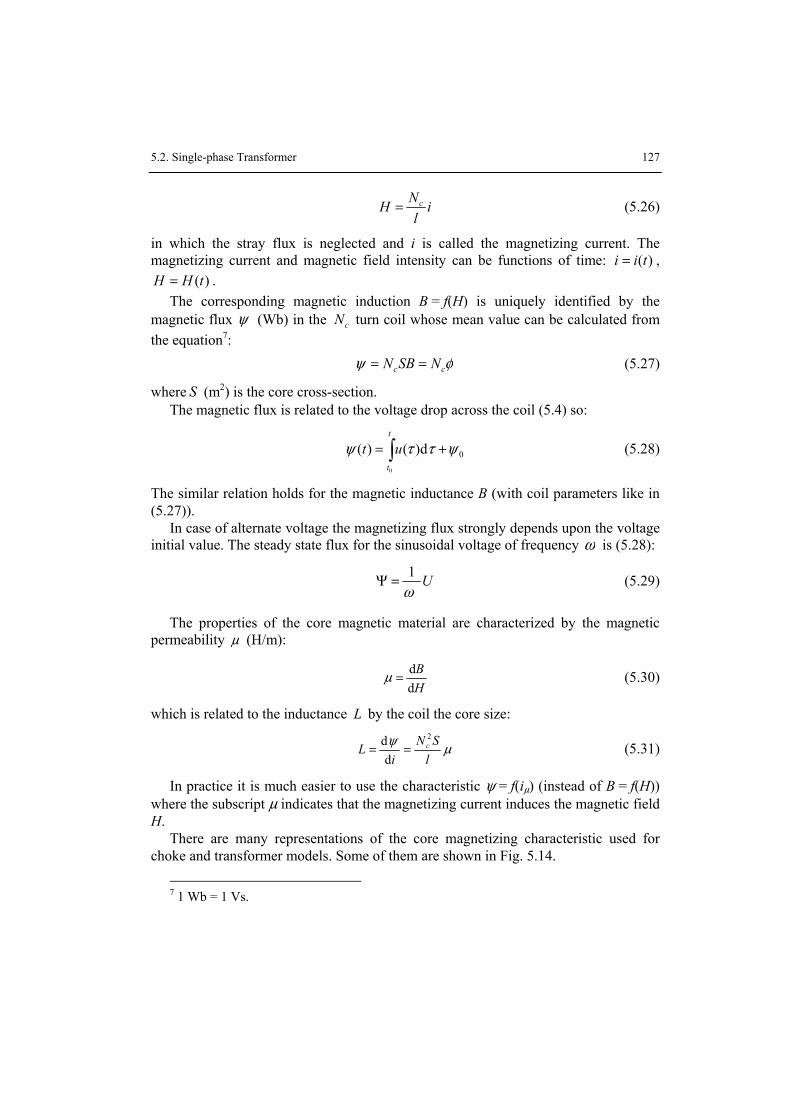
5.2. Single-phase Transformer 127
il
NH c= (5.26)
in which the stray flux is neglected and i is called the magnetizing current. The magnetizing current and magnetic field intensity can be functions of time: )(tii = ,
)(tHH = . The corresponding magnetic induction B = f(H) is uniquely identified by the
magnetic flux ψ (Wb) in the cN turn coil whose mean value can be calculated from the equation7: φψ cc NSBN == (5.27)
where S (m2) is the core cross-section. The magnetic flux is related to the voltage drop across the coil (5.4) so:
0
0
)()( ψττψ += ∫t
t
ut d (5.28)
The similar relation holds for the magnetic inductance B (with coil parameters like in (5.27)).
In case of alternate voltage the magnetizing flux strongly depends upon the voltage initial value. The steady state flux for the sinusoidal voltage of frequency ω is (5.28):
Uω1=Ψ (5.29)
The properties of the core magnetic material are characterized by the magnetic permeability μ (H/m):
HB
dd=μ (5.30)
which is related to the inductance L by the coil the core size:
μψl
SNi
L c2
==d
d (5.31)
In practice it is much easier to use the characteristic ψ = f(iμ) (instead of B = f(H)) where the subscript μ indicates that the magnetizing current induces the magnetic field H.
There are many representations of the core magnetizing characteristic used for choke and transformer models. Some of them are shown in Fig. 5.14.
7 1 Wb = 1 Vs.

128 5. TRANSFORMER MODEL
In simplest case the piecewise approximation of the magnetizing characteristic comprises of three segments for which (Fig. 5.14a): Lμ = 0 (the segment lies on ψ axis) and Lμ = L (two segments for positive and negative values of the magnetizing current). The greater number of segments (Fig. 5.14b) results in the better approximation of the characteristic. The ideal one is the continuous characteristic (Fig. 5.14c).
0 iμ
ψ
0
ψ
0
ψ
0
ψ
a) b)
c) d)
iμ
iμ
iμ
Fig. 5.14. Some representations of the core magnetizing characteristic
The magnetizing characteristic can be approximated by a continuous function and resulting model is called a true type one. The approximation is obtained by use of odd functions, for instance:
...)( 55
331 +++= μμμμψ iaiaiai , (5.32)
and good result is obtained of the first two terms of the series (a1 ≠ 0 and a2 ≠ 0). Inclusion of losses due to the hysteresis and more accurate approximation of losses
in the core can be obtained for the characteristic with the hysteresis loop (Fig. 5.14d), which can also have the piecewise approximation. The function like in (2.41) can be used for this purpose:
( )( ) μμμψ iaIiaai c 321 arctg)( +±⋅= (5.33)
where Ic denotes the magnetizing current corresponding to coercion Hc. If Ic > 0, then the function enables the coarse approximation of the hysteresis loop including the inner loops (the sign depends upon the sign of ψ/dt).

5.2. Single-phase Transformer 129
Accurate approximation of effects in the ferromagnetic core in transient state is difficult [15, 85] and it is important that the model includes the initial conditions for induction (B0) or the flux (ψ0).
The initial value of the flux determines the point on the inner loop (Fig. 5.15a).
0
ψ
iμ
a)
ψ0
ψr
b)
0
ψ
iμ
ψ0
Fig. 5.15. Initial condition in the model: a) with hysteresis and b) without hysteresis
In the model without hysteresis the initial conditions can not be set directly (the magnetizing characteristic passes through the origin – Fig. 5.15b). The problem can be solved by introduction of the voltage source which is active in the first calculation step. The following example shows how the problem is solved in ATP–EMTP.
Example 5.2. Using the ATPDraw interface set up the protection CT model in which the magnetizing characteristic is represented by 98 (pseudo-nonlinear) element with the option of setting the flux initial value.
Let’s consider the 5P208 type CT of the following parameters: nominal power: nS = 20 VA ( nnn ZIS obc
22= ),
nominal load impedance: nZobc = 20 Ω, ϕcos = 0.5, current ratio: 500:1 ( nn II 21 : ) A/A, winding turn ratio: 500:1 ( 12 : NN ), the core cross-section: S = 28.8cm2 = 2.88⋅10–3 m2, the length of magnetic loop: l = 0.675 m, the secondary resistance winding: R2 = 4.5 Ω. The magnetizing characteristic is shown in Fig. 5.16. The characteristic has been obtained experimentally (by measurement) for sinusoidal excitation and the respective values are the peak ones. It must be noted that such a characteristic is not accurate for large values of inductance since the corresponding magnetic field intensity H is calculated for r.m.s. values of current which is strongly distorted; the professional computer programs use the special correcting procedures [24].
8 Protection CT of composite error 5% at rated accuracy limit primary current and Standard
Accuracy Limit Factor 20 [46, 47].
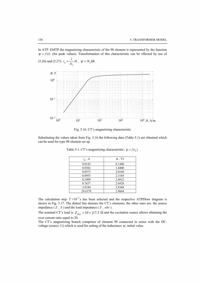
130 5. TRANSFORMER MODEL
In ATP–EMTP the magnetizing characteristic of the 98 element is represented by the function )(if=ψ (for peak values). Transformation of this characteristic can be effected by use of
(5.26) and (5.27): HNli
2
=μ , .2SBN=ψ
100 101 102 103 10410–2
10–1
100
H, A/m
B, T
Fig. 5.16. CT’s magnetizing characteristic
Substituting the values taken from Fig. 5.16 the following data (Table 5.1) are obtained which can be used for type 98 element set up.
Table 5.1. CT’s magnetizing characteristic: )( μψ if=
μi , A ψ , Vs
0.0143 0.1440 0.0382 1.4400 0.0573 2.0160 0.0955 2.3184 0.1909 2.4912 0.7637 2.6928 3.8184 2.8368
28.6378 2.9664 The calculation step T =10–5 s has been selected and the respective ATPDraw diagram is shown in Fig. 5.17. The dotted line denotes the CT’s elements; the other ones are: the source impedance ( SZ _ ) and the load impedance ( obcZ _ ). The nominal CT’s load is j17.310obc +=nZ Ω and the excitation source allows obtaining the over-current ratio equal to 20. The CT’s magnetizing branch comprises of element 98 connected in series with the DC. voltage (source 11) which is used for setting of the inductance .ψ initial value.

5.2. Single-phase Transformer 131
UZ_S
I
Z_2
X_m
UI
P S
:n 1
Z_obc
UI
Fig. 5.17. The circuit with the CT model
The secondary current 2i waveform along with the magnetizing current μi and the flux ψ waveforms are shown in Fig. 5.18 for two values of the remnant flux: 0ψ = 2 Vs (Fig. 5.18a) and 0ψ = 0 (Fig. 5.18b).
Fig. 5.18. The result of CT’s switch-on: a) for remnant flux 0ψ = 2 Vs and b) for zero remnant flux
Basing on (5.28) the external voltage source is switched on at ton = 0 (TSTART = 0) and switched off after one calculation step at toff = ton + T (TSTOP= ε+T , where ε is the fraction
132 5. TRANSFORMER MODEL
of T– the declared time interval of the voltage source activation must be slightly longer than T; otherwise the source will not be switched on. The peak value of U is calculated from (5.28) written in discrete form for one calculation step: UT=ψ from which: TU r /ψ= where: rψ – the initial value of the remnant flux.
5.3. Three-phase Transformer
5.3.1. Two-winding Transformer
The properties of the three-phase transformer depend on arrangement of the windings connection which is called the winding connection group and on the transformer core design. In majority of applications the transformer windings are connected in Δ or in Y arrangement.
The transformer windings are assumed to be symmetrical that implies the identical winding equivalent parameters. Moreover, in the low frequency range (up to. 2000 Hz) the transformer capacitances (phase-to-phase and phase-to-ground) as well as the skin effect can be neglected.
Just like for the single phase transformer the three-phase unit can be considered as a multi-terminal element or as the circuit corresponding to the transformer design with distinguished primary and secondary side. Further, the multi-terminal approach to the transformer winding connection will be presented.
The transformer winding connections are normalized according to respective standards and, generally, different winding connection groups are applied to different power networks [36, 91]. Some of them are shown in Table 5.2.
Knowing the transformer winding arrangement the transformer model can easily be developed. The equivalent circuit of the transformer in Yd11 connection is shown in Fig. 5.19a. The equivalent circuits of the respective winding pairs are the same as for the single-phase transformer. Due to the LS winding connection the LS voltage vectors lead the HS voltage vectors by 30˚. The Y side voltage is equal to the phase one while the Δ side voltage is the phase-to-phase one. Thus, the winding turn ratio is 3 times greater.
The transverse (magnetizing) branch can be connected to any side of the transformer. In ATP–EMTP the magnetizing branch is always connected to the primary side of the transformer model.
The considered representation of the three phase transformer is acceptable if the magnetic circuit configuration allows splitting of the transformer into three separate phase units. It can be done for units with magnetic core as shown in Fig. 5.20b.
The magnetic core design in the three phase transformer determines the transformer properties, in particular, the equivalent representation for the zero sequence component. This component produces the magnetic flux which has the same
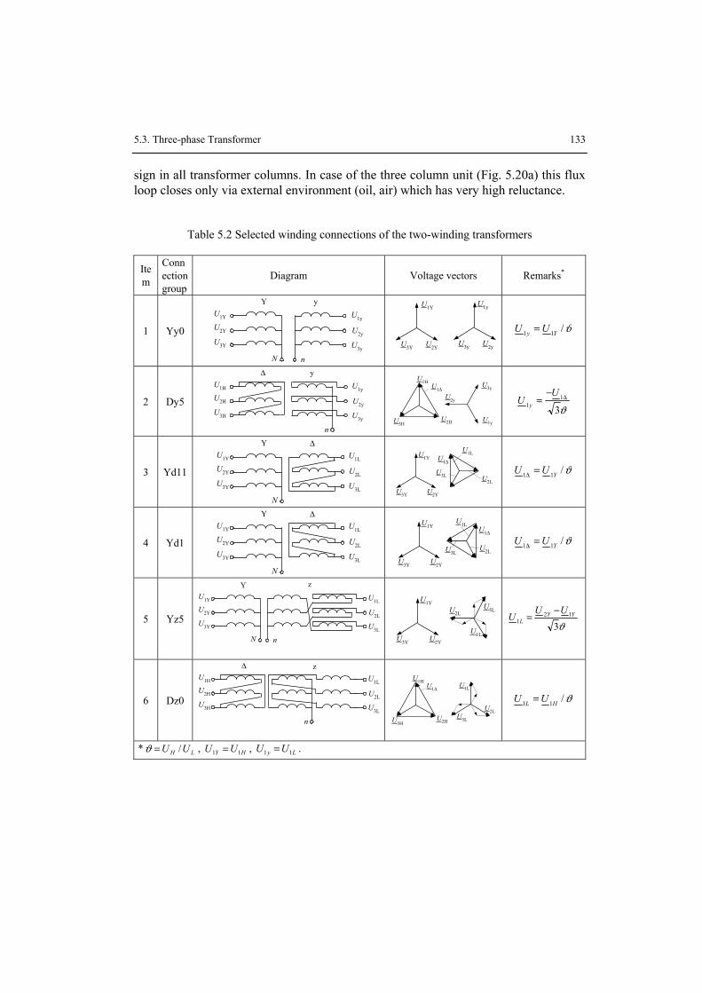
5.3. Three-phase Transformer 133
sign in all transformer columns. In case of the three column unit (Fig. 5.20a) this flux loop closes only via external environment (oil, air) which has very high reluctance.
Table 5.2 Selected winding connections of the two-winding transformers
Item
Connection group
Diagram Voltage vectors Remarks*
1 Yy0
Y y
N n
U1Y
U2Y
U3Y
U1y
U2y
U3y
U1Y
U2YU3Y
U1y
U2yU3y
ϑ/11 Yy UU =
2 Dy5
Δ y
n
U1H
U2H
U3H
U1y
U2y
U3y
U1H
U2HU3HU1y
U2y
U3yU1Δ
ϑ31
1Δ−
=U
U y
3 Yd11
YU1Y
U2Y
U3Y
U1L
U2L
U3L
N
Δ
U1Δ
U1L
U2L
U3L
U1Y
U2YU3Y
ϑ/11 YUU =Δ
4 Yd1
YU1Y
U2Y
U3Y
U1L
U2L
U3L
N
Δ
U1Δ
U1L
U2LU3L
U1Y
U2YU3Y
ϑ/11 YUU =Δ
5 Yz5
Y zU1Y
U2Y
U3Y
U1L
U2L
U3L
N n
U1Y
U2YU3Y
U3L
U1L
U2L
ϑ3
121
YYL
UUU
−=
6 Dz0
Δ zU1H
U2H
U3H
U1L
U2L
U3L
n
U1H
U2HU3H
U1Δ
U3L
U1L
U2L
ϑ/11 HL UU =
* LH UU /=ϑ , HY UU 11 = , Ly UU 11 = .

134 5. TRANSFORMER MODEL
RY LY RΔLΔNY : NΔ
RFe Lμ
iL1H
iL2H
iL3H
iL1L
iL2L
iL3L
L1H
L2H
L3H
L1L
L2L
L3L
N
u1Δu1Y
u2Δu2Y
u3Δu3Y
U1Y
U2YU3Y
U1Δ U2Δ
U3Δ
UL1L
UL2L
UL3L
uL1H
uL2H
uL3H
uL1L
uL2L
uL3L
b)
a)
Fig. 5.19. The equivalent circuit of the Yd11 transformer
The magnetizing characteristic of such magnetic loop is more flat as compared to the ferromagnetic core characteristic and the nonlinearity effect is reduced. In effect the magnetizing inductance for zero sequence component μ0L is much lower. The four and five column transformers (Fig. 5.20b) are devoid of this effect since the zero sequence flux loop closes via additional columns.
Similarly to the single phase transformer the magnetizing circuit can be represented by the nonlinear magnetizing branch as shown in Fig. 5.20 [87]. In case of the three column transformer the effect of the zero sequence flux loop can be modelled by additional circuit as shown in Fig. 5.21.

5.3. Three-phase Transformer 135
uL1L uL2L uL3L
uL1H uL2H uL3H
uL1L uL2L uL3L
uL1H uL2H uL3H
a) b)
Fig. 5.20. The three phase transformer cores: a) three column, b) five column
Due to the different magnetic loops for the positive and zero sequence flux components the three column transformer impedance for the latter is 3 – 5 times greater [8].
Using two extra ideal transformer of 1:1 turn ratio (Fig. 5.21) the triple value of the zero sequence voltage 3u0Hμ at transformer HS is obtained. The triple nonlinear inductance represents the magnetic circuit for the zero sequence flux component.
RY LY RΔLΔNY : NΔ
Lμ
iL1H
iL2H
iL3H
L1H
L2H
L3H
L1L
L2L
L3L
N
3L0μ
1:1
1:1
iL1L
iL2L
iL3L
i0H
3u0Ημ
Fig. 5.21. The equivalent circuit of the Yy0 transformer with the three column core
In ATP–EMTP the input data format for this model is determined by TRANSFORMER THREE PHASE (TRAYYH_3 in ATPDraw interface). The relevant details are illustrated by the following example.

136 5. TRANSFORMER MODEL
Example 5.3. Using the ATPDraw graphical interface set up the model of the 110/20 kV power system fragment with 40 MVA Yn0y0 three column transformer (Y/Y with earthed HS and unearthed LS - Fig. 5.22).
Zs
Za Zb
Es 110kV 15km20kVTr
Fig. 5.22. The diagram of the modelled power system fragment
The transformer parameters: nominal power: nS = 40 MV⋅A; nominal voltage: 115/22 kV. the following parameters have been measured at the transformer LS: For the positive sequence component: loses in the core: pPFeΔ = 32 kW; magnetizing current: pIμ = 11.4 A; magnetizing voltage pUμ = 19.0 kV; load loses in windings: CuPΔ = 205 kW; short-circuit current: NHz II = = 200.8 A; short-circuit voltage: zU = 12.07 kV; For the zero sequence component: loses in the core: pP 0FeΔ = 168.1 kW; magnetizing current: pI 0μ = 280 A ; magnetizing voltage: pU 0μ = 1.636 kV (voltage at the short-circuited LS terminals); load loses in windings: pP 0CuΔ = 12.5 kW; short-circuit current: pzI 0 = 95 A; source impedance: sZ1 = 0.15+j2.5 Ω, sZ0 = 0.26+j3.4 Ω; loading power: aS _obc = 25.4+j15.8 VA, bS _obc = 4.5+j2.2 MVA. The magnetizing characteristic for LS is shown in Table 5.3). The 20 kV overhead line: The line length l = 15 km; 1R = 0.36 Ω/km; 1X = 0.38 Ω/km; 0R = 0.60 Ω/km;
0X = 1.55 Ω/km; 1C = 10.5 nF/km; 0C = 4.2 nF/km. The data are necessary to set up the transformer model (TRAYYH_3 in ATPDraw). The following calculations are automatically carried out by the program:

5.3. Three-phase Transformer 137
2.1319224.11 ===
p
Np U
UIIμ
μμ A, 9.42192232
22
=⎟⎠⎞
⎜⎝⎛=⎟
⎟⎠
⎞⎜⎜⎝
⎛Δ=Δ
p
NFepFe U
UPPμ
kW.
Subscript p indicates that the measurements were not taken in nominal conditions so, assuming that the circuit is linear, the nominal values are recovered.
Table 5.2. The magnetizing characteristic )( μψ if= for LS (22kV)
μi , A ψ , Vs
18.62 57.20 38.95 64.56 367.6 75.27 1121.0 77.97 3587.0 80.43
The same for the zero sequence:
6.7243636.1
223
28033 0
00 ===
p
Np
UUI
Iμ
μμ A,
101333636.1
221.1683
22
000 =⎟⎟
⎠
⎞⎜⎜⎝
⎛=
⎟⎟
⎠
⎞⎜⎜
⎝
⎛Δ=Δ
p
Np U
UPPμ
FeFe kW.
The measured magnetizing current pIμ and magnetizing voltage pUμ determine the linear part of the magnetizing characteristic )( μψ if= . The respective values are:
12.1624.112 === pIi μμ A, ( ) ( ) 38.493314/2190003/2 === ωψ μpU Vs.
The values are used for calculation of the magnetizing branch reactance:
μμ
ωψi
X = ,
which, in turn, is used for calculation of the initial steady state of the network. The transformer impedance can be determined from measurement data obtained in the short-circuit conditions:
695.18.2003
2050003 22
Cu =⋅
=Δ=z
T IPR Ω, 7.34
32008.007,12
3===
z
zT I
UZ Ω,
66.34695.17.34 2222 =−=−= TTT RZX Ω. and the respective winding parameters are:
8475.02/ == TH RR Ω, 35.172/ == TH XX Ω,
031.011522 2
=⎟⎠⎞
⎜⎝⎛= HL RR Ω, 635.0
11522 2
=⎟⎠⎞
⎜⎝⎛= HL XX Ω.

138 5. TRANSFORMER MODEL
As the losses in iron for positive and zero components are different they can not be represented by the resistor connected in parallel with the inductance Lμ (Fig. 5.21). The losses can be represented by the external three phase element of mutually coupled resistors connected to the transformer terminals. The resistance matrix of that element can be determined from the symmetrical components relation:
32 10 FeFe
FeRR
R S+
= , 3
10 FeFeFe
RRR M
−= ,
where: 4810001.168
636.133 2
0Fe
20
0Fe =⋅=Δ
=p
p
PU
R μ Ω, 11281100032
1922
1 ==Δ
=p
p
PU
RFe
Feμ Ω.
Thus: 8.7536311281248
Fe =⋅+=SR Ω, 0.374431128148
Fe −=−=MR Ω.
These resistances are calculated with respect to the L-side and form the following matrix:
⎥⎥⎥
⎦
⎤
⎢⎢⎢
⎣
⎡
−−−−−−
=⎥⎥⎥
⎦
⎤
⎢⎢⎢
⎣
⎡=
8.75360.37440.37440.37448.753637440.37440.37448.7536
R
FeFeFe
FeFeFe
FeFeFe
Fe
SMM
MSM
MMS
RRRRRRRRR
Ω.
Using the ATPDraw interface the coupled resistors in form of the type 51, 52, 53 elements are connected to the transformer model by default [7]. The constant zero sequence inductance L0μ is represented by the reluctance at the LS of the transformer:
( )μ0
2
0 33/
LUR NL
m = .
The inductance L0μ can be estimated from the equation:
3/
1
0
00
0p
NH
T
NLp
IZZ
II
UL
μ
μμ
μ ω
⎟⎟⎠
⎞⎜⎜⎝
⎛−
= , where NL
NNL U
SI3
= , N
NHNH S
UZ2
= represent the base values at the
primary and the secondary side of the transformer, respectively (Fig. 5.21). Substituting the necessary data we get:
0517.03/280π100
6.3307.34
7.10496.72411636
0 =⋅
⎟⎠⎞
⎜⎝⎛ −
=μL H, and: ( ) 10390517.09
223
3/22 2
0
2
0 =⋅
==μL
Rm Ω.
The neutral point earthing resistance RNg. is determined as the difference between power losses for zero and positive sequence components measured in the transformer winding:
CuCu PPPNg Δ−Δ=Δ 0 , where 57.5023/958.2005,12
3/
22
00Cu0Cu =⎟
⎠⎞
⎜⎝⎛=⎟⎟
⎠
⎞⎜⎜⎝
⎛Δ=Δ
z
zp I
IPP kW (referred to
the nominal current). Thus: 27.2970.20527.502 =−=Δ NgP kW.
The earthing resistance value is:

5.3. Three-phase Transformer 139
( )23 NH
NgNg I
PR
Δ= =
( )82.0
8.2003297270
2 =⋅
=NgR Ω.
In ATPDraw interface the resistance is included by default. The load impedance is calculated from the equation:
*0
2
SUZ N
O = (the asterisk denotes the conjugate value). Further:
06.7j35.118.15j4.25
202
_ +=−
=aobcZ Ω, 07.35j74.712.2j5.4
202
_ +=−
=bobcZ Ω.
The load impedance is represented by the RLCY3 element while the line is modelled by use of the three phase Π circuit with the following matrices R, X, C:
32 10 RRRS
+= , 3
10 RRRM−= , where: 0.96.0150 =⋅=R Ω, 4.536.0151 =⋅=R Ω. From that:
6.6=SR Ω, 2.1=MR Ω.
Similarly, the line reactance is: 25.2355.1150 =⋅=X Ω, 5738.0151 =⋅=X Ω, 55.11=SX Ω, 85.5=MX Ω.
The line capacitances are represented by the respective susceptances ( fCCB π2== ω , 50=f Hz):
79.19102.415π100 30 =⋅⋅⋅= −B μS, 48.49105.1015π100 3
1 =⋅⋅⋅= −B μS.
58.393
48.49279.1932 10 =⋅+=+= BBBS μS, 97.9
379.1948.49
301 −=−=−= BBBM μS.
The ATPDraw model of the system considered is shown in Fig. 5.23. The primary side current waveforms calculated for the transformer switch-on in ‘no load’ conditions are presented in Fig. 5.24. The highest voltage in phase L1 results in very small value of the magnetizing current in this phase. The currents in other phases are biased in the same direction (positive or negative half-waves) so the content of the second harmonic is very large in these currents.
I VH L
MI
I
Fig. 5.23. ATPDraw model of the system considered
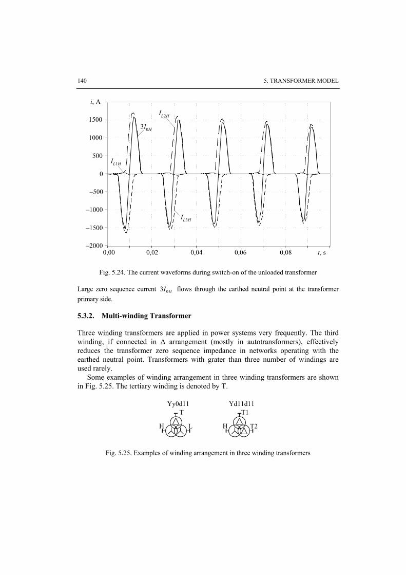
140 5. TRANSFORMER MODEL
0,00 0,02 0,04 0,06 0,08 t, s–2000
–1500
–1000
–500
0
500
1000
1500
i, A
3I0H
IL1H
IL2H
IL3H
Fig. 5.24. The current waveforms during switch-on of the unloaded transformer
Large zero sequence current HI03 flows through the earthed neutral point at the transformer primary side.
5.3.2. Multi-winding Transformer
Three winding transformers are applied in power systems very frequently. The third winding, if connected in Δ arrangement (mostly in autotransformers), effectively reduces the transformer zero sequence impedance in networks operating with the earthed neutral point. Transformers with grater than three number of windings are used rarely.
Some examples of winding arrangement in three winding transformers are shown in Fig. 5.25. The tertiary winding is denoted by T.
T
H L
Yy0d11T1
H T2
Yd11d11
Fig. 5.25. Examples of winding arrangement in three winding transformers

5.3. Three-phase Transformer 141
The three phase three winding transformer model can be obtained by connection of three single winding three phase transformer models (s. 123). If one of the windings is in Δ arrangement then the impact of the zero sequence component flux can be neglected9. The example 5.4 shows how the three winding transformer model is realized in ATP–EMTP.
Example 5.4. Using the ATPDraw interface set up the model of the 220/110/10 kV power system fragment with Yn0yn0d11 160 MVA transformer (Fig. 5.26). The load at MV side (10 kV) is So = 32 + j18 MV⋅A. and the secondary winding load is S2 = 105 + j28 MV⋅A. The other system parameters are as below.
The transformer parameters: nominal power: rTrLrH SSS // = 160/160 /50 MV⋅A; nominal voltage: 230/120/10,5 kV; short-circuit voltage: %10=KHLu , %5.33=KHTu , %8.20=KLTu (referred to HS); idle current: %5.00 =i ; losses in the core: %25.0Fe =ΔP ; winding resistance: 320/80/2.4 mΩ; source impedance: sHZ1 =0.35+j3.77 Ω, sHZ0 =1.16+j10.42 Ω; sLZ1 =0.18+j1.55 Ω,
sLZ0 =0.56+j2.75 Ω.
ZsHEsH 220kV 110kV
Tr
EsL
10kVZsL
ZO
Fig. 5.26. The system diagram
The magnetizing characteristic (the relative values) is as in Table 5.4.
The turn ratio calculation:
9.215,10
230 ===rT
rHHT U
Uϑ , 92.1120230 ===
rL
rHHL U
Uϑ .
9 The zero sequence voltage at the Y side which induces the flux is small since the Δ
winding enhances the zero sequence current flow at the YN side.
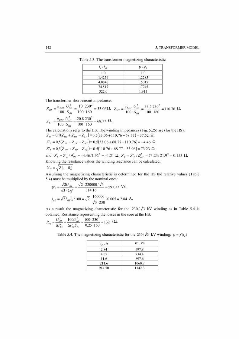
142 5. TRANSFORMER MODEL
Table 5.3. The transformer magnetizing characteristic
0/ μμ ii 0/ψψ
1.0 1.0 1.4259 1.2285 4.0846 1.5015 74.517 1.7745 322.0 1.911
The transformer short-circuit impedance:
06.33160230
10010
100
22
===rH
rHKHLHL S
UuZ Ω, 76.110160230
1005.33
100
22
===rH
rHKHTHT S
UuZ Ω,
77.68160230
1008.20
100
22
===rH
rHKLTLT S
UuZ Ω.
The calculations refer to the HS. The winding impedances (Fig. 5.25) are (for the HS): ( )LTHTHLH ZZZZ −+= 5,0 = ( ) 52.3777.6876.11006.335.0 =−+ Ω,
( )HTLTHLL ZZZZ' −+= 5,0 = ( ) 46.476.11077.6806.335.0 −=−+ Ω,
( )HLLTHTT ZZZZ' −+= 5,0 = ( ) 23.7306.3377.6876.1105.0 =−+ Ω,
and: 21.192.1/46.4/ 22 −=−== HLLL Z'Z ϑ Ω, 153.09.21/23.73/ 22 === HTTT Z'Z ϑ Ω. Knowing the resistance values the winding reactance can be calculated:
22HHH RZX −=
Assuming the magnetizing characteristic is determined for the HS the relative values (Table 5.4) must be multiplied by the nominal ones:
77.59716.314
3/230000223
20 =⋅=
⋅=
fU rH
πψ Vs,
84.2005.02303
1600002100/2 00 =⋅⋅
⋅== iIi rHμ A,
As a result the magnetizing characteristic for the 3/230 kV winding as in Table 5.4 is obtained. Resistance representing the losses in the core at the HS:
13216025,0
230100100 222
=⋅
⋅=Δ
=Δ
=rH
rHrH
SPU
PUR
FeFeFe
kΩ.
Table 5.4. The magnetizing characteristic for the 3/230 kV winding: )( μψ if=
μi , A ψ , Vs
2.84 597.8 4.05 734.4 11.6 897.6
211.6 1060.7 914.50 1142.3

5.3. Three-phase Transformer 143
The load impedance for MV (10 kV) network (Δ arrangement):
47.1j62.218j32
5.10 22+=
+==
o
rTo S
UZ Ω.
In case of the three winding transformer the reactance of one winding is negative what may bring about the numerical stability problems. That is why the magnetizing branch should be connected to one of the transformer terminals but to the neutral point (Fig. 5.19). In our case this is HS winding [17]. The considered model diagram is shown in Fig. 5.27. The transverse branches are represented by TYPE-98 (pseudo-nonlinear reactor) elements which in ATPDraw are denoted as NLININD.
RHY LHY
RFe Lμ
RLYLLY
NH
RTΔLTΔ
NL
iL2L
iL1L
iL3L
iL1T
iL2T
iL3T
iL1H
iL3H
iL2H
L2L
L1L
L3L
L1T
L2T
L3T
L1H
L2H
L3H
Fig. 5.27. The considered transformer model

144 5. TRANSFORMER MODEL
The power system model is shown in Fig. 5.28. To stabilize the model the unearthed 10 kV winding is connected to the earth via 10 nF capacitors (corresponding susceptance 10.87 μS) in each phase. Being equivalent to few tens of meters of cable feeder the capacitors do not essentially change the system operating conditions.
I
SAT
Y Y
I
I
I
I
Fig. 5.28. The ATPDraw model of the analysed system
0,00 0,02 0,04 0,06 0,08 t, s
iH, A
–7000
–5000
–3000
–1000
1000
3000iL1
iL3iL2
Fig. 5.29. Current waveforms at the HS of the transformer
The magnetizing branches are connected to the earthing resistor 0.1=NR Ω at the HS of the transformer. The L1–G fault at the 110 kV bus-bar was simulated via fault resistance 5.0=zR Ω. For this purpose the splitter was used. The respective current waveforms are shown in Fig. 5.29.

5.3. Three-phase Transformer 145
The multi winding transformer model can be applied to modelling of winding internal faults. In such case the faulty winding is divided into two parts and fault model is connected to the winding fault location. Using the ATPDraw interface transformer models the faulty winding division must be done in all three phases. Thus modelling the internal winding fault in two winding transformer the three phase one must be used in which two in series connected windings make one winding of the two winding transformer.
5.3.3. Z (zig-zag)-connected Transformer
The HV/MV transformers usually operate in Yd arrangement with adequate phase shift. In order to get the possibility of MV side neutral point earthing (for instance, via Peterson coil or resistor) the special earthing transformers are used. In such transformers the earthing windings are connected in Z arrangement (zig-zag – Table 5.2) in order to minimize the transformer zero sequence impedance value. The windings connection can provide positive or negative phase shift (Fig. 5.30). In general, Z connected windings may have different number of turns and the resulting relations are [40, 41]:
– turn ratio:
( )ααϑ
−===
3/sinsinπz
y
z
yz U
UNN
(5.34)
a)
UL1
UL2
UL3
n
UL1
UL2
UL3
n
UL1
UL2
UL3
UL3
UL1
UL2
UzUy U3y
U1z
U2y
U1z
UzUy
α
α
b)
I1z
I2y
I1z
I3y
Fig. 5.30. Zig-zag connections

146 5. TRANSFORMER MODEL
– voltage vector relation in the first phase:
3/πj1
1 e1 pz
Lz
UUϑ+
= (5.35)
3/πj
3/πj1
e1e
pz
pzL
kyUU
ϑϑ
+= (5.36)
where p denotes the sign which for positive phase shift (Fig. 5.30a) is also positive (p = 1, index k = 2). For negative phase shift (Fig. 5.30b) p = –1, index k = 3.
In the equivalent circuit the winding resistance is proportional to the turn number and the reactance of in series connected winding is proportional to the squared turn number. Thus, ( yz RRR += , yz XXX += ):
z
zRRϑ+
=1
, z
zy
RRϑ
ϑ+
=1
, (5.37)
21 zz
XXϑ+
= , 2
2
1 z
zy
XXϑϑ
+= (5.38)
The magnetizing current is measured for unloaded transformer and can be determined for any winding. In case of the first phase the magnetizing current is related to the first core column and can be determined from the equation μμ XUI L j/1= . The losses in core iron can be neglected. Using the first part of the winding the magnetizing current is:
z
zz X
UIIμ
μμ j1== (5.39)
The second winding on the same column refers to the phase L3 and the related magnetizing current is:
3/21 πjej z
y
yy I
XU
I μμ
μ == (5.40)
Equations (5.39) and (5.40) are valid for the transformer with positive phase shift (Fig. 5.30a). For negative phase shift the sign of power in (5.40) must be changed. Multiplying (5.40) by zϑ and subtracting (5.39) from (5.40) we get:
( )y
yz
z
zzz X
UX
UIμμ
μ ϑϑjj
e πj 113/21 −=− (5.41)

5.3. Three-phase Transformer 147
where: zzy XX μμ ϑ 2= . Applying this relation along with (5.35), (5.36) and (5.38) to (5.41) we get the final formulas [40]:
21 zzz
XX
ϑϑμ
μ ++= , 2
2
1 zz
zy
XX
ϑϑϑμ
μ ++= (5.42)
which enable to calculate the magnetizing branch reactance from the measured reactance μX .
In similar way the magnetizing reactance for zero sequence component can be determined. The zero sequence currents in windings on the same column flow in the same direction and bear the opposite signs so, by analogy to (5.39) and (5.40), equation (5.41) takes the form:
( )0
0
0
00 1
y
yz
z
zz X
UXUI
μμϑϑ
jj−=− (5.43)
where: 0zU , 0yU – the zero sequence voltage on the respective windings; 0zX μ , 0yX μ – the respective zero sequence magnetizing reactances.
Equations analogous to (5.35), (5.36) and (5.38) applied to (5.43) yield:
( )20
00 1
2
zz I
UXϑμ −
= , ( )2
2
0
00 1
2
z
zy I
UXϑϑ
μ −= (5.44)
where: 0U , 0I – the r.m.s. values of the zero sequence voltage and current at the transformer Z terminals.
Note that for 1=zϑ (both windings have the same number of turns) the zero sequence magnetizing reactance tends to infinity (no magnetizing branch). The transformer impedance, as ‘seen’ from point n (Fig. 5.30), is very small (equal to the winding resistance and the stray reactance only).
The phase shift 6/π±=α of the earthing transformer can be adjusted in ‘hour’ steps (0, 6, 5, 11,…) depending on how the third winding is connected.
Changing the ratio zϑ the phase shift α of any arbitrary value can be obtained. This property is applied in design of three winding Zdy transformers which supply
the electronic power converters. In such application the transformer is supplied from the Z winding side and the phase shift value between Δ and Y windings is selected to minimize ripples in the 12-pulse converter d.c. output current. [40]. The winding connection diagram of such a transformer along with the vector diagram are shown in Fig. 5.31. In ATPDraw interface such a transformer is modelled by use of SATTRAFO block and the input data can be calculated from equations presented in this paragraph.

148 5. TRANSFORMER MODEL
ZL1
ZL2
ZL3
DL1
YL1
DL2
YL2
DL3
YL3
NZ NY
UZL1
UZL2
UZL3
U1z α
UYL1
UYL2
UYL3
UDL1UDL2
UDL3
a) b)
Fig. 5.31. Transformer ZNd11y: a) wiring diagram, b) voltage vector diagram
Exercises
5.1. Show the winding connection diagrams for the two winding transformers in the following connection groups: a) Yd5 b) Zy5 c) Zy11 d) Dz6 e) Dd6 f) Yy6 g) Dd0 h) Dy11
5.2. In Example 5.3 the modelling procedure for the three column Yy0 transformer is shown. The presented magnetizing characteristic (Table 5.3) refers to the LS (22 kV) of the transformer. Rescale that characteristic for the HS (115 kV) of the transformer.
5.3. The LS winding of the Yy0 transformer in Example 5.3 has been rearranged into Δ connection thus making the new Yd1 unit. Calculate the LS nominal voltage of the new transformer for which the original magnetizing characteristic doesn’t have to be re-scaled. Set up the ATPDraw model of the new transformer using the original transformer data. Carry out the relevant comparison tests.

Exercises 149
5.4. Below the results of the magnetizing characteristic measurement for the LS winding of the Yd1 transformer are shown. The transformer parameters are:
3.6=rS MVA, 11/115=rU kV, =Δ CuP kW, =Δ FeP kW, 8.00 =i %. Measurement results:
I, A U, kV 1.53 11.0 2.86 12.1 9.55 13.2 28.6 13.7 107.9 14.3
Determine the characteristic )( μψ if= which can be used in ATP–EMTP (peak values).
Note: In ATP–EMTP such calculations can be carried out using SATURA subroutine. As the input data the relative values of the original characteristic (as above) must be entered (voltage and current referred to the nominal values for the winding considered)– see file satur1.dat.
5.5. Set up and examine the transformer Zy5 20/0,5kV model of the following parameters: rHS =630kV⋅A, rLS =100 kV⋅A, ku = 4.5%, CuPΔ =1.5% (referred to rLS ). The short-
circuit power at the 20 kV busbar zS = 6000 MV⋅A. The neutral point at the SN side is earthed via resistor and at the LS is earthed solidly. Determine by experiment the earthing resistance value for which the short-circuit current at the 20 kV busbar for the phase–to-ground fault is equal to 100 A r.m.s.


6. MODELLING OF ELECTRIC MACHINES
In this Chapter rotating electric machines are analysed. It is assumed that the Reader knows the basic theory of electric machines design and operation. Electric machines, due to the magnetic coupling between the stator and the rotor windings, are similar to the transformer. However, since the rotor winding is in continuous motion with respect to the stator ones the analysis of the electric machine is more complex.
The presented here analysis is limited to the synchronous and the AC induction (asynchronous) electric machines operating as electric motors or as power generators.
6.1. Synchronous Machines
The basic functional diagram of an electric machine is shown Fig. 6.1. The electric machine design details may differ significantly depending mainly on the applied rotating velocity of the machine rotor. This velocity is related to the power network frequency f1 by the following equation:
601npf = (Hz), (6.1)
where: n – the rotating velocity of the rotor, (1/min), p – the number of pole pairs.
N
S
A
A
B
B C
C
UA
UC
UB
Fig. 6.1. The functional diagram of a three phase rotating electric machine; p = 1

152 6. MODELLING OF ELECTRIC MACHINES
The factor n/60 (Hz) in (6.1) is the rotating velocity of the electric machine shaft. Multiplication of the machine pole pair number results in adequate increase of the electric and magnetic quantities related to the rotating magnetic field produced by the machine rotor. For example, if the angular speed of the magnetic field in the machine γe changes p times faster than the angular speed of the rotor γr then:
re pγγ = (6.2)
In case of cylindrical rotor with a single pair of poles (as in turbo generators) the rotor speed is equal to 3000 rotates/min (for the network fundamental frequency of 50 Hz). The power generators driven by the water turbines (hydro generators) usually rotate with the lower speed so they must have the greater number pole pairs.
6.1.1. Model in 0dq Coordinates
a) Electric Part
The machine shown in Fig. 6.1 can be represented by the equivalent diagram comprising of four separate circuits as shown in Fig. 6.2. The three-phase circuit represents the stator windings. If the stator windings are connected in star arrangement the neutral point can be earthed directly or via impedance The excitation winding is represented by the circuit of the equivalent parameters fr , fL and is supplied by the external d.c. voltage fu .
Fig. 6.2. The equivalent circuits of the synchronous machine

6.1. Synchronous Machine 153
The other two circuits represent the damping windings located at the machine rotor. The damping windings are meant for suppression of the rotor oscillatory swings which occur in transient states. These equivalent (and in fact dummy) circuits are located in the main rotor ( Dr , DL ) axis and in the vertical one ( Qr , QL ). In case of relatively low power units (up to a few MVA) the excitation flux is generated by permanent magnet rotors thus improving the machine reliability and efficiency.
The stator windings can be connected in star or in delta arrangement. The three following circuits are related with the machine stator: the excitation circuit driven by the external source to produce the magnetic field and the two equivalent D and Q circuits. The current and voltage directions (arrows) are shown in Fig. 6.2 for the stator and rotor windings.
All the circuits are mutually coupled (the equivalent damping circuits are short-circuited) and represent sort of a transformer which can be described by the following equations [10, 24]:
tddψRiu −−= (6.3)
where:
⎥⎥⎥⎥⎥⎥⎥⎥
⎦
⎤
⎢⎢⎢⎢⎢⎢⎢⎢
⎣
⎡
−=
00
f
C
B
A
uuuu
u ,
⎥⎥⎥⎥⎥⎥⎥⎥
⎦
⎤
⎢⎢⎢⎢⎢⎢⎢⎢
⎣
⎡
=
Q
D
f
C
B
A
iiiiii
i ,
⎥⎥⎥⎥⎥⎥⎥⎥
⎦
⎤
⎢⎢⎢⎢⎢⎢⎢⎢
⎣
⎡
=
Q
D
f
C
B
A
ψψψψψψ
ψ ,
⎥⎥⎥⎥⎥⎥⎥⎥
⎦
⎤
⎢⎢⎢⎢⎢⎢⎢⎢
⎣
⎡
=
Q
D
f
C
B
A
rr
rr
rr
R ,
and, assuming that the circuit is linear, the particular fluxes are proportional to the values of currents:
⎥⎥⎥⎥⎥⎥⎥⎥
⎦
⎤
⎢⎢⎢⎢⎢⎢⎢⎢
⎣
⎡
⎥⎥⎥⎥⎥⎥⎥⎥
⎦
⎤
⎢⎢⎢⎢⎢⎢⎢⎢
⎣
⎡
=
⎥⎥⎥⎥⎥⎥⎥⎥
⎦
⎤
⎢⎢⎢⎢⎢⎢⎢⎢
⎣
⎡
Q
D
f
C
B
A
QQQDQfQCQBQA
DQDDDfDCDBDA
fQfDfffCfBfA
CQCDCfCCCBCA
BQBDBfBCBBBA
AQADAfACABAA
Q
D
f
C
B
A
iiiiii
LLLLLLLLLLLLLLLLLLLLLLLLLLLLLLLLLLLL
ψψψψψψ
(6.4)
or, in compact form:

154 6. MODELLING OF ELECTRIC MACHINES
⎥⎦
⎤⎢⎣
⎡⎥⎦
⎤⎢⎣
⎡=⎥
⎦
⎤⎢⎣
⎡
fDQ
ABC
rrs
srs
fDQ
ABC
ii
LLLL
ψψ
(6.5)
in which the quantities related to the rotor and stator are separated. However, since the rotor turns, reluctances for particular magnetic fluxes change. In effect the inductances in the machine equations depend on the rotor angle position γ (Fig. 6.3):
iLψ )(γ= (6.6)
and:
00
γτωγγ +== ∫t
e d (6.7)
where: )(te ωωω == – electric angular velocity, γ0 – the initial value of γe. It should be noted that the rotor angular velocity depends on the pole pair number
and, by analogy to (6.2):
p
er
ωω = (6.8)
The equation (6.8) is characteristic for synchronous machines in which the rotor and stator magnetic field rotation velocities are the same in the steady state. The rotor synchronous rotation velocity is p times lesser.
Analysis of the diagram in Fig. 6.3 leads to the following equations for the stator inductance matrix LS elements:
γ2cosMSAA LLL += , ⎟⎠⎞
⎜⎝⎛ −+=
3π22cos γMSBB LLL , ⎟
⎠⎞
⎜⎝⎛ ++=
3π22cos γMSCC LLL ,
⎟⎟⎠
⎞⎜⎜⎝
⎛⎟⎠⎞
⎜⎝⎛ ++−==
6π2cos γMSBAAB LMLL ,
⎟⎟⎠
⎞⎜⎜⎝
⎛⎟⎠⎞
⎜⎝⎛ −+−==
2π2cos γMSCBBC LMLL ,
⎟⎟⎠
⎞⎜⎜⎝
⎛⎟⎠⎞
⎜⎝⎛ ++−==
6π52cos γMSACCA LMLL ,
where: LM, LS, MS are the constant inductances; γ is the angle between the rotor main axis d and the magnetic field axis of A taken as the reference.
In dq coordinates the axis d leads the axis q and such arrangement is in accordance with the adopted standards of synchronous machine analysis [10, 24].
Inductance LM appears in model of machines with salient poles; for machines with cylindrical rotors LM = 0.

6.1. Synchronous Machine 155
d
q
γ
A
C
B
LAA
LCC
LBB
δLf
LD LQ
directionof rotation
Fig. 6.3. the equivalent diagram of synchronous machine
The stator and rotor mutual inductances can be determined in the similar way:
γcosffAAf MLL == , ⎟⎠⎞
⎜⎝⎛ −==
3π2cos γffBBf MLL , ⎟
⎠⎞
⎜⎝⎛ +==
3π2cos γffCCf MLL ,
γcosDDAAD MLL == , ⎟⎠⎞
⎜⎝⎛ −==
3π2cos γDDBBD MLL ,
⎟⎠⎞
⎜⎝⎛ +==
3π2cos γDDCCD MLL ,
γsinQQAAQ MLL == , ⎟⎠⎞
⎜⎝⎛ −==
3π2sin γQQBBQ MLL , ⎟
⎠⎞
⎜⎝⎛ +==
3π2sin γQQCCQ MLL .
The self- and mutual inductances of the rotor do not depend upon its angular position and the inductances of vertically laid windings are equal to zero:
RDffD MLL == , 0== QffQ LL , 0== QDDQ LL .
The parameter matrix in (6.4) and (6.5) is symmetrical ( Trssr LL = ).
The machine model described by (6.3)–(6.7) is called the natural one or the machine model in phase coordinates. The model parameters are time-varying what is clearly noticeable after substitution of (6.6) into (6.3):

156 6. MODELLING OF ELECTRIC MACHINES
tt dd
dd iLiLRiu )()( γγ −−−= (6.9)
Numerical solution of (6.9) is cumbersome and sometimes essential for the natural machine model feasibility.
Simplification of the problem is obtained by replacement of coordinates attached to the machine stator by the coordinates attached to the revolving rotor. The coordinates are determined by mutually vertical axes d–q. This approach is known as the Park’s transformation. The third coordinate is related to the zero sequence component and is taken into account if the stator windings neutral point is earthed. The stator currents and voltages are transformed into 0dq coordinates in the following way:
ABCdq
ABCdq
uPu
iPi
)(
)(1
0
10
γ
γ−
−
=
= (6.10)
where: ⎥⎥⎥
⎦
⎤
⎢⎢⎢
⎣
⎡
=
q
ddq
iii0
0i , ⎥⎥⎥
⎦
⎤
⎢⎢⎢
⎣
⎡
=
q
ddq
uuu0
0u .
The same relation can be written for the magnetic flux. Matrix )(γP contains coefficients which project the stator phase quantities onto d–
q axes of the revolving rotor. The zero sequence components are like in standard symmetrical component transformation:
⎥⎥⎥⎥⎥⎥⎥
⎦
⎤
⎢⎢⎢⎢⎢⎢⎢
⎣
⎡
⎟⎠⎞
⎜⎝⎛ +⎟
⎠⎞
⎜⎝⎛ −
⎟⎠⎞
⎜⎝⎛ +⎟
⎠⎞
⎜⎝⎛ −=−
3π2sin
3π2sinsin
3π2cos
3π2coscos
21
21
21
32)(1
γγγ
γγγγP (6.11)
The constant normalizing coefficient has been introduced to make the matrices orthogonal:
[ ]
⎥⎥⎥⎥⎥⎥⎥
⎦
⎤
⎢⎢⎢⎢⎢⎢⎢
⎣
⎡
⎟⎠⎞
⎜⎝⎛ +⎟
⎠⎞
⎜⎝⎛ +
⎟⎠⎞
⎜⎝⎛ −⎟
⎠⎞
⎜⎝⎛ −== −
32sin
32cos
21
32sin
32cos
21
sincos2
1
32)()( 1
ππ
ππ
γγ
γγ
γγ
γγ TPP (6.12)

6.1. Synchronous Machine 157
and to simplify the inverse transformation:
dqABC
dqABC
0
0
)(
)(
uPu
iPi
γγ
=
= (6.13)
since now the normalizing coefficients used for both transformations are the same. Substitution of (6.13) into (6.3) with reference to (6.4) and (6.5) leads to the
following equation:
⎪⎭
⎪⎬⎫
⎪⎩
⎪⎨⎧
⎥⎦
⎤⎢⎣
⎡⎥⎦
⎤⎢⎣
⎡−⎥
⎦
⎤⎢⎣
⎡⎥⎦
⎤⎢⎣
⎡⎥⎦
⎤⎢⎣
⎡−=⎥
⎦
⎤⎢⎣
⎡⎥⎦
⎤⎢⎣
⎡
fDQ
dq
fDQ
dq
fDQ
ABC
fDQ
dq
t ψψ
1P
ii
1P
rr
uu
1P 000 )()()( γγγ
dd (6.14)
and further:
⎥⎦
⎤⎢⎣
⎡⎥⎦
⎤⎢⎣
⎡+
⎪⎭
⎪⎬⎫
⎪⎩
⎪⎨⎧
⎥⎦
⎤⎢⎣
⎡−⎥
⎦
⎤⎢⎣
⎡⎥⎦
⎤⎢⎣
⎡−=⎥
⎦
⎤⎢⎣
⎡
fDQ
dq
fDQ
dq
fDQ
dq
fDQ
ABC
fDQ
dq
t ψψ
0Ω
ψψ
ii
rr
uu 0000
dd (6.15)
where matrix:
⎥⎥⎥
⎦
⎤
⎢⎢⎢
⎣
⎡−==
−
010100000
)()(1
ωγγ PPΩtd
d (6.16)
is the rotation matrix [30]. Note that resistance matrix R being diagonal remains unchanged after
transformation. Moreover, it can be assumed that resistances in all phases are identical:
sCBA rrrr === .
To facilitate calculations (6.15) is represented using the machine resistance and inductance R L parameters. Substituting (6.13) into (6.5) we get:
⎥⎦
⎤⎢⎣
⎡⎥⎦
⎤⎢⎣
⎡⎥⎦
⎤⎢⎣
⎡=⎥
⎦
⎤⎢⎣
⎡⎥⎦
⎤⎢⎣
⎡
fDQ
dq
rrs
srs
fDQ
dq
ii
1P
LLLL
ψψ
1P 00 )()( γγ
, and further:
⎥⎦
⎤⎢⎣
⎡⎥⎦
⎤⎢⎣
⎡=⎥
⎦
⎤⎢⎣
⎡ −−
fDQ
dq
rTsr
srs
fDQ
dq
ii
LPLLPPLP
ψψ 0
110
)()()()(
γγγγ
(6.17)
The inductance matrix in (6.17):

158 6. MODELLING OF ELECTRIC MACHINES
⎥⎥⎥⎥⎥⎥⎥⎥
⎦
⎤
⎢⎢⎢⎢⎢⎢⎢⎢
⎣
⎡
=⎥⎦
⎤⎢⎣
⎡=
DRD
Rff
Dfd
rTsr
srT
sT
E
LMkLMMkMLMk
MkLMkMkL
L
0000000000
000000000000
)()()()(
1
1
1
1
11
0
LPLLPPLP
Lγ
γγγ (6.18)
is constant and time invariant and:
SS MLL 20 −= , MSSd LkMLL 21++= , MSSq LkMLL 2
1−+= , 2/31 =k . Moreover, the normalized form of matrix P(γ) makes the inductance matrix
symmetrical thus facilitating the respective numerical calculation procedures. Finally, (6.17) can be written in the following compact form:
EEE iLψ = (6.19)
where: ⎥⎦
⎤⎢⎣
⎡=
fDQ
dqE ψ
ψψ 0 , ⎥
⎦
⎤⎢⎣
⎡=
fDQ
dqE i
ii 0 .
Relations between electric quantities in 0dq model of electric machine are presented graphically in Fig. 6.4. In similar compact form (6.15) can be written:
ωuuRiψ +−−= EEE
tdd
(6.20)
or:
( )ωuuRiLi +−−= −EEE
E
t1
dd , (6.21)
where:
⎥⎦
⎤⎢⎣
⎡=
fDQ
dqE u
uu 0 ,
⎥⎥⎥⎥
⎦
⎤
⎢⎢⎢⎢
⎣
⎡−=
0
ud
q
ωψωψ
ω
0
,
QQqqq iMkiL 1+=ψ , ( )DDffddd iMiMkiL ++= 1ψ .

6.1. Synchronous Machine 159
LD
rDiD
LQ
rQiQ
Lf
rfif
uf
Ld
ra id
ud
ωψq
Lq
ra iq
uq
ωψd
L0
r0 i0
u0
stator winding rotor winding
k1Mf
k1MD
MR
k1MQ
Fig. 6.4. Graphical representation of synchronous machine for 0dq coordinates
Equations (6.20) – in flux notation or (6.21) – in voltage notation, along with (6.10) and (6.13), define the electric part of the synchronous machine for 0dq coordinates (Fig. 6.4). The angular velocity ω in (6.21) refers to magnetic field changes and is related to the rotor angular velocity according to (6.8) which describes the coupling between electrical and mechanical part of the machine model.
The presented model can be modified according to actual needs (simplification of calculations, better representation of electromagnetic effects). In order to obtain the identical coefficients of mutual inductance the transformation ratios between windings in d axis can be modified [24]:
adRDf LMMM === 2/32/3 . The modification is effective for correct turn numbers in particular windings. The
first equation ( Df MM = ) can easily be satisfied since the damping winding is

160 6. MODELLING OF ELECTRIC MACHINES
dummy. The second one is true for corrected turn number of the excitation winding which can be calculated from the following relations:
fm
fm ikk
i1
1= , fmfm kk ψψ 1= , fmfm ukku 1= , (6.22)
where: R
fm M
Mk = .
The modification also requires the adequate rescaling of the excitation current value what can be done outside of the model.
Due to the modification the equivalent voltages in the coupled magnetic circuits (Fig. 6.4) are the same so the circuits can be directly connected. As a result the equivalent circuits as shown in Fig. 6.5 are obtained. Splitting (6.21) into three parts respectively related to 0dq coordinates we get:
LDm–MmrDmiDm
rQmiQm
rfmifm
ufm rsm id
ud
ωψqm
rsm iq
uq
ωψdm
L0 r0 i0
u0
Mm
Lfm–Mm
MQm
LQm–MQm
Ld–Mm
Lq–MQm
Fig. 6.5. The equivalent circuit diagram of the synchronous machine for 0dq coordinates

6.1. Synchronous Machine 161
⎟⎟⎟
⎠
⎞
⎜⎜⎜
⎝
⎛
⎥⎥⎥
⎦
⎤
⎢⎢⎢
⎣
⎡−+
⎥⎥⎥
⎦
⎤
⎢⎢⎢
⎣
⎡−−
⎥⎥⎥
⎦
⎤
⎢⎢⎢
⎣
⎡
⎥⎥⎥
⎦
⎤
⎢⎢⎢
⎣
⎡−
⎥⎥⎥
⎦
⎤
⎢⎢⎢
⎣
⎡=
⎥⎥⎥
⎦
⎤
⎢⎢⎢
⎣
⎡−
00
0
1qm
fm
d
Dm
fm
d
Dm
fm
s
Dmmm
mfmm
mmd
Dm
fm
d
uu
iii
rr
r
LMMMLMMML
iii
t
ωψ
dd
(6.23)
⎟⎟⎠
⎞⎜⎜⎝
⎛⎥⎦
⎤⎢⎣
⎡+⎥
⎦
⎤⎢⎣
⎡−⎥
⎦
⎤⎢⎣
⎡⎥⎦
⎤⎢⎣
⎡−⎥
⎦
⎤⎢⎣
⎡=⎥
⎦
⎤⎢⎣
⎡−
00
1dmq
Qm
q
Qm
s
QmQm
Qmq
Qm
q uii
rr
LMML
ii
tωψ
dd
(6.24)
0
00
0
00
dd
Lui
Lr
ti −−= , (6.25)
where: QmQmqqq iMiL +=ψ , ( )Dmfmmddd iiMiL ++=ψ , fmm MkkM 2
1= , fmfm LkkL 221= ,
DmDm LkkL 221= , QmQm LkkL 22
1= , QmQm MkkM 21= , fmfm rkkr 22
1= , DmDm rkkr 221= ,
QmQm rkkr 221= .
The coefficient km in (6.22) can be determined by measurements for idle (no load) run of the machine [24] when id = iq = iD = 0 and fmmq iMu ω= . Then, using (6.22), we can write:
G
fmNm Uk
iMk
1
01
3ω
=mN
fmG
MkrU
11
3ω
= , (6.26)
where: UG – the nominal voltage of the generator (r.m.s. phase-to-phase value for stator windings in delta arrangement or r.m.s. phase-to-ground value for stator windings in star arrangement), if 0 – the excitation current for machine idle run.
It is assumed that the machine model parameters in q axis can be modified by use of the same coefficient km.
More accurate modelling of the machine operation in transient states can be achieved if the greater number of the dummy short-circuited windings is included into the machine model in both (d and q) axes. Having different parameters the windings can model the effects in the machine iron that have different time constants [4, 8, 57].
The parameters rfm i Mm in (6.26) as well as the other ones are determined according to the specified standards [64]. The machine parameters measurements can be carried out both in short-circuit and in idle run conditions. Usually the following machine parameters are deemed to be the basic ones [24, 64]:
sR – stator winding resistance;
lX – stator winding stray reactance;
0X – zero sequence reactance of the machine;

162 6. MODELLING OF ELECTRIC MACHINES
dX' , qX' – transient reactance: series and transverse, respectively;
dX'' , qX'' – sub-transient reactance: series and transverse, respectively;
d'τ , q'τ – transient time constants: series and transverse, respectively;
d''τ , q''τ – sub-transient time constant: series and transverse, respectively. The reactances in the list above refer to the nominal frequency, for example,
lNl LX 1ω= while the time constants determine the transient d.c. components decay rate:
RX
RL
N1ωτ == .
Parameters which refer to the open generator circuits (idle run) are denoted by extra ‘o’ in the subscript, for example: do'τ denotes the time constant in d axis for the idly running generator.
The further details concerning the machine model parameters determination can be found in [4, 24, 64].
b) Saturation Consideration
Accurate modelling of magnetic circuit saturation effect in rotating machines is a complex problem which requires the cumbersome analysis of the machine magnetic core design by use of advanced numerical methods like Finite Element Method [123]. Therefore the commonly applied methods of transient state analysis in electric machines are based on the following simplifying assumptions [24, 60]:
– the overall magnetic flux produced by a given winding comprises of the basic and the stray flux only; the saturation intensity of the magnetic material depends upon the value of the overall magnetic flux;
– the stray flux does not get saturated; – the mutual inductance of the rotor is sinusoidal; – the hysteresis and the eddy currents effects are negligible. The magnetizing characteristic of the idly running generator (open stator circuit
while the excitation current is changed at nominal rotation velocity) is necessary for inclusion of the saturation effect into the machine model (see Fig. 6.6 [53]). The characteristic can be continuous or piecewise approximated.
Calculation of saturation effect impact is carried out by iteration process in which the new points on magnetizing characteristics are calculated for all generators present in the analysed network. The process is illustrated in Fig. 6.6. The reference base for inductance calculation is the linear part of the magnetizing characteristic whose slope ml = tan(αl). Let’s assume that the machine working point A1 has been determined in

6.1. Synchronous Machine 163
the current calculation step. The point is located on the linear characteristic whose slope m2 = tan(α2). In the next calculation step the new operating point A2 located on the same linear characteristic is determined along with the new value of the magnetizing current im2. Using this new excitation current value the corrected flux B2 is calculated from the nonlinear magnetizing characteristic.
The resulting inductance correction ratio is: χ2 = m2/ml. According to the simplifying assumptions correction concerns the main flux only, for example:
fdlnasd MkLL 12_ χ+= , (6.27)
where: Ldl – stray inductance along d axis or:
Fig. 6.6. Idle run magnetizing characteristic of the generator
RnasR MM 2_ χ= (6.28)
for the mutual inductance f–D (Fig. 6.4). The algorithm can be modified according to the numerical methods being used for
calculations [24, 53, 60].
c) Mechanical Model
The basic dynamic equation of the machine rotor mechanical balance is as follows:
etrr TT
tD
tJ −=+
dd
dd
2
2 γγ , (6.29)

164 6. MODELLING OF ELECTRIC MACHINES
where: J – inertia torque of the rotating mass, (kg⋅m2)10; D – damping factor, (N⋅m/(rad/s)); tT , eT – turbine (mechanical) and generator (electromechanical) torque, respectively, (N⋅m).
The angle γr is related to rω by (6.7). In case of power generator – tT > eT – turbine energy is transmitted to power system.
Electromagnetic torque of the machine can be determined from (6.9). For )(tii = , )(tγγ = and for ),( γLiLL = , where iL – the current in inductance which is an element
of matrix L11 we get:
ttt
ii
L
L dd
dd
dd iLiLLRiu −⎟⎟
⎠
⎞⎜⎜⎝
⎛∂∂+
∂∂−−= γ
γ (6.30)
Multiplying (6.30) by vector iT the instantaneous machine power is obtained:
eLRG PPPP −−−= (6.31)
where:
uiTGP = – output power, (6.32)
RiiTRP = – power loss in windings, (6.33)
⎟⎟⎠
⎞⎜⎜⎝
⎛∂∂+
∂∂+=⎟
⎠⎞
⎜⎝⎛
∂∂=
∂∂= iLiLiLiiLi
tti
itttEP L
L
TTLL d
ddd
dd γ
γ21
21 – magnetizing power, (6.34)
EL – energy of electromagnetic field,
rerTT
e Tpt
P ωωγ
γγ
=∂∂=
∂∂= iLiiLi
221
dd – electromagnetic power. (6.35)
The electromagnetic torque in the air slot between stator and rotor is given by the equation:
iLi ⎟⎟⎠
⎞⎜⎜⎝
⎛=γd
dTe
pT2
(6.36)
where i is the vector of phase currents in stator and rotor and L is like in (6.6). Using 0dq coordinates (6.36) reduces to [9]:
( )dqqde iipT ψψ −= (6.37)
10 Inertia torque is also expressed in (N⋅m⋅s2); 1 kg⋅m2 = 1 N⋅m⋅s2. 11 Important for nonlinear magnetic circuits where inductance is a function of current.

6.1. Synchronous Machine 165
The remarks concerning the physical interpretation of discussed relations are: • Signs of particular powers in (6.31) correspond to current and voltage notation
in Fig. 6.5. • The magnetizing power PL is produced by each magnetic field change while Pe
is related to the rotor rotation (changing angle γ). • The zero sequence component (6.37) does not affect the electromagnetic
torque. Sometimes, instead of inertia torque, the inertia constant H is used and:
N
N
SEH = ,
MVAsMW
VAsW ⋅=⋅ 11 (6.38)
where: 62 10
21 −×= rNN JE ω (MW⋅s) – energy of rotating mass12;
rNω – nominal (synchronous ) rotor angle velocity (1/s);
NS – nominal apparent power (MVA). Thus:
N
rN
SJH
62 105.0 −×= ω =N
N
SnJ 2
9104831.5 ⋅× − (s) (6.39)
where π2
60 rNNn ω= – nominal rotating velocity (rot/min).
Equation (6.29) and definition (6.38) show that for nominal driving torque Tt = TtN, (N⋅m) at D = 0 machine will attain the nominal rotation velocity after time τm = 2H (s) (parameter τm is sometimes called the mechanical time constant [57] or the running in time. The inertia torque J in (6.29) can be expressed by parameters which are easier to obtain:
62 10×⋅=rN
Nm SJω
τ = 62 102 ×⋅
rN
NSHω
= 62 10378.182 ×⋅⋅
N
N
nSH (6.40)
and the dynamic equation of the machine can be rewritten as:
gtr
rNr
rN
N PPt
Dtf
SH −=+⋅d
dd
dπ
γωγ2
2
(6.41)
where: rNf – nominal rotor frequency (Hz); tP , gP – turbine and generator power (MW), respectively.
12 1 W⋅s = 1 N⋅m = 1 J.

166 6. MODELLING OF ELECTRIC MACHINES
The time constant τm takes the values from the range 1–20 s depending on the size and the nominal power of the machine.
If the rotating system contains several masses linked by resilient couplings then the mechanical torque conveyed is proportional to the angle displacement between particular elements (Fig. 6.7). In such a multi-section arrangement couplings convey the resilience torque sT to adjacent elements so the torque signs have to be differentiated accordingly. In general case we have [24]:
( ) isiiiiis TKT ,1,11, −=−= −−− γγ (6.42)
where: iiK ,1− – the resilience coefficient between rotating masses i–1, i. The damping in particular elements also has to be differentiated as the 'self-' and
the mutual one. The latter represents losses caused by the resilient link swings and can be expressed by the following equation:
( ) ( )11,1,1, ++−− −+−+= iiiiiiiii
iid tD
tD
tDT γγγγγ
dd
dd
dd (6.43)
where: iiD ,1− , 1, +iiD – damping coefficients in couplings between respective masses. In the system shown in Fig 6.7 sections 1–3 generate the driving torque (in
direction of the system rotation) while sections 4–5 are those driven ones. Using (6.42) and (6.43) the multi-mass system equation takes the form:
1
T1
J1
T2
D12
2
K12 J2
T3
D23
3
K23 J3
T4
D34
4
K34 J4
T5
D45
5
K45 J5
driving units load units
Fig. 6.7. Diagram of the multi-stage rotating system
etttTTKγγDγJ −=++
dd
dd
2
2
, (6.44)
where: J – diagonal matrix of inertia torque (J1, J2, ..., Jn) for particular elements; γ – vector of angles (γ1, γ2, ..., γn) for particular elements; K – matrix of the resilience coefficients:
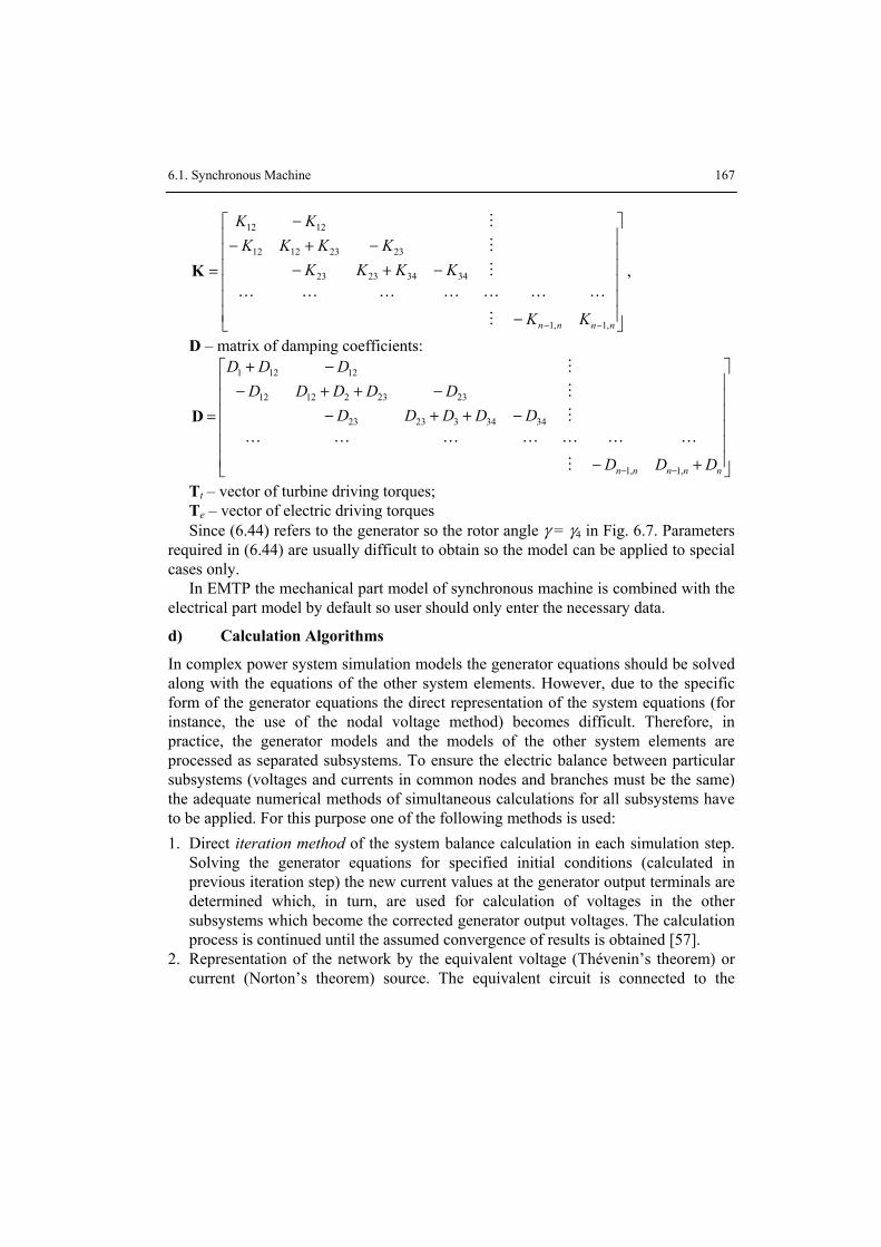
6.1. Synchronous Machine 167
⎥⎥⎥⎥⎥⎥
⎦
⎤
⎢⎢⎢⎢⎢⎢
⎣
⎡
−
−+−−+−
−
=
−− nnnn KK
KKKKKKKK
KK
,1,1
34342323
23231212
1212
M
LLLLLLL
M
M
M
K ,
D – matrix of damping coefficients:
⎥⎥⎥⎥⎥⎥
⎦
⎤
⎢⎢⎢⎢⎢⎢
⎣
⎡
+−
−++−−++−
−+
=
−− nnnnn DDD
DDDDDDDDDD
DDD
,1,1
343432323
232321212
12121
M
LLLLLLL
M
M
M
D
Tt – vector of turbine driving torques; Te – vector of electric driving torques Since (6.44) refers to the generator so the rotor angle γ = γ4 in Fig. 6.7. Parameters
required in (6.44) are usually difficult to obtain so the model can be applied to special cases only.
In EMTP the mechanical part model of synchronous machine is combined with the electrical part model by default so user should only enter the necessary data.
d) Calculation Algorithms
In complex power system simulation models the generator equations should be solved along with the equations of the other system elements. However, due to the specific form of the generator equations the direct representation of the system equations (for instance, the use of the nodal voltage method) becomes difficult. Therefore, in practice, the generator models and the models of the other system elements are processed as separated subsystems. To ensure the electric balance between particular subsystems (voltages and currents in common nodes and branches must be the same) the adequate numerical methods of simultaneous calculations for all subsystems have to be applied. For this purpose one of the following methods is used: 1. Direct iteration method of the system balance calculation in each simulation step.
Solving the generator equations for specified initial conditions (calculated in previous iteration step) the new current values at the generator output terminals are determined which, in turn, are used for calculation of voltages in the other subsystems which become the corrected generator output voltages. The calculation process is continued until the assumed convergence of results is obtained [57].
2. Representation of the network by the equivalent voltage (Thévenin’s theorem) or current (Norton’s theorem) source. The equivalent circuit is connected to the

168 6. MODELLING OF ELECTRIC MACHINES
generator and solved along with the machine equations. This approach is called the compensation method 13 [12, 24].
3. Representation of electric machines by the equivalent voltage or current sources connected to the system model. The method is known as prediction method [12, 24, 60]. Common calculations ensure balance between both subsystems but some machine quantities must be predicted. The direct iteration method is accurate and stable but due to iterations applied in
each simulation step makes the calculations time-consuming. The compensation method is also accurate but the subsystem with generators must
not contain any true type nonlinear element. In ATP–EMTP this method is used by the model of Universal Machine (UM) [7, 12].
The prediction method is applied in EMTP to simulation of complex networks (Type 59 model) [24].
6.1.2. Model in Phase Coordinates
The basic drawback of the synchronous machine representation in 0dq coordinates is the lack of direct transformation between 0dq and phase coordinates since transformation coefficients depend upon solution which is unknown and use of extrapolations may result in instability of the network model [12].
The generator model in phase coordinates is as follows:
⎥⎦
⎤⎢⎣
⎡−⎥
⎦
⎤⎢⎣
⎡⎥⎦
⎤⎢⎣
⎡−=⎥
⎦
⎤⎢⎣
⎡⎥⎦
⎤⎢⎣
⎡
fDQ
ABC
fDQ
ABC
fDQ
ABC
fDQ
ABC
rrs
srs
t uu
ii
rr
ii
LLLL
)()()()(
γγγγ
dd (6.45)
where the notation is like in (6.3)–(6.7) and usually Lr(γ) = Lr. On the basis of (6.3) the digital model of the generator is developed and is directly
connected to the network model. Both models are solved together. Calculations are carried out according to the following algorithm [12, 13]: 1. Predict the rotor angular velocity ω and the rotor angle position γ. Determine the
equivalent parameters of the generator. 2. Calculate the rotor currents and the electric torque using (6.36). Solving the
equations of the mechanical model the new values of ω and γ are obtained. 3. Check the solution convergence with respect to ω. In case of unacceptable
discrepancy return to p. 2. In EMTP the method is applied in Type-58 generator model [13]. The method is
stable and the nonlinear elements in the network model are acceptable [53, 60].
13 Compare with p. 2.3.2.

6.2. Induction Machines 169
6.2. Induction Machines
6.2.1. General Notes
The name induction machine refers to the wide group of rotating electric machines in which electromagnetic (generators) or electrodynamic (motors) force is produced by magnetic fields induced in stator and rotor. The rotor magnetic field is produced by the current induced in the rotor windings (or short-circuited cages) when the rotor moves in the stator magnetic field. Contrary to synchronous machines the rotor and stator magnetic field frequencies are different and that is why the induction machines are also called the asynchronous ones.
Taking into account the design features induction machines of the following types are used in practice:
1. Cage (or squirrel-cage) rotor electric machines in which the rotor winding is made of cooper or aluminium rods connected at their ends (Fig. 6.8). In case of the cage machine the alternate stator magnetic field induces electric current in the rotor cage and the resulting rotor magnetic flux produces the rotation torque.
Fig. 6.8. Squirrel-cage induction machine model
Stator and rotor magnetic fields rotate in the same direction so the current in rotor cage can be induced when the stator and rotor rotation velocities are different. The difference is defined as the slip s and:
1
1
1
1
ωωω ee
nnns −=−= (6.46)

170 6. MODELLING OF ELECTRIC MACHINES
where: 1n – synchronous rotation velocity (angular velocity 1ω ), en – rotor filed rotation velocity (rotor field angular velocity eω ).
In the machine with pole pairs number p > 1:
re pωω = (6.47)
where rω - rotor angular velocity and:
p
sr
)1(1 −= ωω (6.48)
The current in symmetrical rotor winding has the frequency:
6011 r
rn
ss
psff
−== (Hz) (6.49)
where rn = n – rotation velocity (rot/min). The value of slip depends upon machine operating state. At the beginning of machine starting s =1 and decreases gradually to the value 0>s which depends on machine load. In case of induction power generator 0<s .
To facilitate the machine starting (to get the greater torque for reduced inrush current) the machine rotors are modified by application of multi-cage and deep bar rotor designs (Fig. 6.9).
Such designs take advantage of the skin effect properties to increase the rotor resistance during machine inrush when the machine slip is big.
a) b) c)
Fig. 6.9. Examples of rotor design: a) normal, b) deep, c) double cage
2. Wound-rotor machines in which standard windings (in star or delta arrangement) are connected to slip rings (Fig. 6.10).

6.2. Induction Machines 171
stator rotor
Fig. 6.10. Slip ring machine model.
Such design essentially facilitates the machine inrush process since the external variable resistances can be connected in series with the rotor windings. The value of the start controlling resistances, being large at the beginning of machine starting, is gradually reduced to zero when machine rotation speed increases [6, 10].
3. Doubly-fed induction machine design is similar to the wound-rotor machine one; here the slip rings are used for connection of external excitation source of specified frequency so the machine rotation speed (in motor) or the output voltage frequency (in generator) can be controlled [9]. In some conditions the doubly-fed machines behave like the synchronous ones. Mutual reaction of rotor and stator magnetic fields of frequencies rsf and rf , respectively, fixes the ‘synchronous’ rotation speed at the value determined by slip according to (6.46).
6.2.2. Mathematical Model
Induction and synchronous machine models are very much alike. The voltage equation in phase coordinates for a single three phase rotor winding is like in (6.3):
⎥⎦
⎤⎢⎣
⎡−⎥
⎦
⎤⎢⎣
⎡⎥⎦
⎤⎢⎣
⎡−=⎥
⎦
⎤⎢⎣
⎡− )(
)(
)(
)(
)(
)(
rABCr
sABC
rABCr
sABC
rr
s
rABCr
sABC
t ψψ
ii
RR
uu
dd (6.50)
where the extra ‘r’ subscript indicates the rotor winding. The rotor winding voltages can be different from zero in doubly-fed machines.
Magnetic fluxes produced by stator (s) and rotor windings (r) can be determined by the following equation:

172 6. MODELLING OF ELECTRIC MACHINES
⎥⎦
⎤⎢⎣
⎡⎥⎦
⎤⎢⎣
⎡=⎥
⎦
⎤⎢⎣
⎡
)(
)(
)(
)(
rABCr
sABC
rrs
srs
rABCr
sABC
ii
LLLL
ψψ
(6.51)
where the inductance matrices comprise of the following sub-matrices:
⎥⎥⎥⎥⎥⎥
⎦
⎤
⎢⎢⎢⎢⎢⎢
⎣
⎡
−−
−−
−−
=
ssMsMs
Msss
Ms
MsMsss
s
LLL
LLL
LLL
22
22
22L ,
⎥⎥⎥⎥⎥⎥
⎦
⎤
⎢⎢⎢⎢⎢⎢
⎣
⎡
−−
−−
−−
=
rrMrMr
Mrrr
Mr
MrMrrr
r
LLL
LLL
LLL
22
22
22L ,
⎥⎥⎥⎥⎥⎥⎥
⎦
⎤
⎢⎢⎢⎢⎢⎢⎢
⎣
⎡
⎟⎠⎞
⎜⎝⎛ −⎟
⎠⎞
⎜⎝⎛ +
⎟⎠⎞
⎜⎝⎛ +⎟
⎠⎞
⎜⎝⎛ −
⎟⎠⎞
⎜⎝⎛ −⎟
⎠⎞
⎜⎝⎛ +
=
γγγ
γγγ
γγγ
cos3π2cos
3π2cos
3π2coscos
3π2cos
3π2cos
3π2coscos
srsr LL , Tsrrs LL = ,
and:
r
ssrMs N
NLL = , s
rsrMr N
NLL = , Msslss LLL += , Mrrlrrr LLL += ,
slL , rlrL – stator and rotor stray inductance, respectively,
srL – magnitude of mutual inductance between stator and rotor windings,
sN , rN – number of turns in stator and rotor, respectively, γ = γe – electric angle between stator and rotor coordinates. To simplify the machine equivalent model the rotor circuit voltages can be
transformed to the level of the stator windings ones. The relevant transformation formulas are [10]:
)()()()(
222
,1
,,,
rABCrsrrABCrABCrsr
rABC
sr
rrr
sr
rlrrl
Ms
Mrsr
Ms
srsr
kk
kRR
kLL
LLk
LLk
iiuu ==
==== (6.52)
The next step towards the induction machine model simplification is the transformation of the stator and rotor phase coordinates into the 0dq ones:
⎥⎦
⎤⎢⎣
⎡⎥⎦
⎤⎢⎣
⎡+
⎪⎭
⎪⎬⎫
⎪⎩
⎪⎨⎧
⎥⎦
⎤⎢⎣
⎡−⎥
⎦
⎤⎢⎣
⎡⎥⎦
⎤⎢⎣
⎡−=⎥
⎦
⎤⎢⎣
⎡− )(0
)(0
)(0
)(0
)(0
)(0
)(0
)(0
)(0
)(0
rdq
sdq
rdq
sdq
rdq
sdq
rdq
sdq
rdq
sdq
t ψψ
0Ω
ψψ
ii
RR
uu
dd (6.53)

6.2. Induction Machines 173
where the angular velocity in the matrix Ω (6.16) is the rotor electric velocity: ω = pωr; )(0 sdqψ , )(0 rdqψ denote the stator (s) and rotor (r) magnetic fluxes in 0dq coordinates – like in (6.17):
⎥⎦
⎤⎢⎣
⎡⎥⎦
⎤⎢⎣
⎡⎥⎦
⎤⎢⎣
⎡⎥⎦
⎤⎢⎣
⎡=⎥
⎦
⎤⎢⎣
⎡−
−
)(0
)(01
1
)(0
)(0
00)(
00)(
rdq
sdq
rTsr
srs
rdq
sdq
ii
CP
LLLL
CP
ψψ γγ
(6.54)
in which matrix C represents relation between phase (ABC) and 0dq rotor coordinates. Elements of vector u0dq(r) are different from zero for the slip-ring machines (Fig.
6.10); in cage machines the rotor circuits are short-circuited. The transformation matrix )(γP is like in (6.11); γ is the electric angle and can be calculated from (6.7) for ω = pωr so, that:
erpt
ωωγ ==dd (6.55)
Matrix C–1 transforms the three phase quantities in the rotor winding into 0dq coordinates and is related to the matrix )(γP by the following equation:
⎥⎥⎥
⎦
⎤
⎢⎢⎢
⎣
⎡
−⋅
⎥⎥⎥⎥⎥⎥⎥
⎦
⎤
⎢⎢⎢⎢⎢⎢⎢
⎣
⎡
−−
−=⋅=γγγγγγ
cossin0sincos0
001
23
21
21
23
21
21
012
1
32)()( ECP (6.56)
Matrix C is known as the transformation matrix between three phase and 0αβ coordinates in normalized form (4.81). Matrix E(γ) represents the angular displacement (rotation) of stator coordinates with respect to the rotor ones - axis d leads the axis q – like in the synchronous machine model (Fig. 6.3). Transformation of three phase stator and rotor quantities into 0dq coordinates is given by the equations:
)(
1)(
)(11
)(1
)( )(
rABCrodq
sABCsABCsodq
iCi
iCEiPi
⋅=
⋅⋅=⋅=−
−−− γ (6.57)
for currents and, by strict analogy, for other quantities. Substituting (6.57) to (6.54) we get:
⎥⎦
⎤⎢⎣
⎡⎥⎦
⎤⎢⎣
⎡=⎥
⎦
⎤⎢⎣
⎡
)(0
)(0
)(0)(0
)(0)(0
)(0
)(0
rdq
sdq
rdqT
srdq
srdqsdq
rdq
sdq
ii
LLLL
ψψ
(6.58)

174 6. MODELLING OF ELECTRIC MACHINES
where:
⎥⎥⎥
⎦
⎤
⎢⎢⎢
⎣
⎡
=
qs
ds
s
sdq
LL
L0
)(0L , ⎥⎥⎥
⎦
⎤
⎢⎢⎢
⎣
⎡
=
qr
dr
r
rdq
LL
L0
)(0L , ⎥⎥⎥
⎦
⎤
⎢⎢⎢
⎣
⎡
=
qsr
dsrsrdq
LL
0
)(0L .
Taking into account the assumed symmetry of stator and rotor windings the equality of the model parameters can be verified:
mqsrdsr LLL == , mslsqsds LLLLL +=== , mrlrqrdr LLLLL +=== (6.59)
where: slL , rlL – stray inductances of the stator and rotor windings unified to the common level.
Resistance matrices in 6.53) can be determined using the transformation matrices )(γP and C. Symmetry of the stator and rotor windings implies that:
⎥⎥⎥
⎦
⎤
⎢⎢⎢
⎣
⎡=
s
s
s
sdq
RR
R
)(0R , ⎥⎥⎥
⎦
⎤
⎢⎢⎢
⎣
⎡=
r
r
r
rdq
RR
R
)(0R (6.60)
where: )(sAR = )(sBR = )(sCR = sR , )(rAR = )(rBR = )(rCR = rR . Equations (6.53) and (6.54) describe the induction machine model in 0dq
coordinates attached to rotor. The machine equations for particular coordinates are simple (diagonal parameter matrices) since d i q coordinates are mutually vertical.
Let’s consider in more detail the voltage equations of the equivalent stator and rotor circuits for d coordinate:
( ) ( )( )
( )t
iLt
iLLiRu
iLiLLt
iLt
iLLiRu
dsm
drmrldrrdr
qrmqsmsldr
mds
msldssds
dd
dd
dd
dd
+++=
+++−+−−= ω (6.61)
Subtraction of (6.61) results in the voltage equation of the equivalent machine circuit along d axis:
( )( )
( ) drqrmqssdr
rlds
sldrrdss
drqrmqsmsldr
rlds
sldrrdssds
uiLiLt
iLt
iLiRiR
uiLiLLt
iLt
iLiRiRu
+++−−−−=
++++−−−−=
ω
ω
dd
dd
dd
dd
(6.62)
In the similar way the voltage equation along q axis can be derived:
( ) qrdrmdssqr
rlqs
slqrrqssqs uiLiLt
iL
ti
LiRiRu ++−−−−−= ωd
dd
d (6.63)

6.2. Induction Machines 175
and also for zero sequence component:
t
iLiRut
iLiRu rrlrrr
sslsss d
dd
d 000
000 , −−=−−= (6.64)
The respective equivalent circuit diagrams are shown Fig. 6.11 in which:
drdsdm iii −= , qrqsqm iii −= (6.65)
Rrl iqrRsiqs
uqs
ωψds
Lm
LrlLsl
b)
iqm
uqr
Rrl idrRsids
uds
ωψqs
Lm
LrlLsl
a)
idm
udr
Rsi0s
u0s
Lslc) Rri0r
u0r
Lrl
Fig. 6.11. Equivalent circuit diagram of induction machine: a) for d axis, b) for q axis and c) for zero sequence components
Connection of the discussed model to the model of the external network requires inverse transformation of calculated quantities into phase coordinates as ‘seen’ at the real machine terminals in each simulation step.
In case of slip-ring machines the starting resistance has to be included into the overall rotor resistance. The model equations have to be modified for other than considered number of rotor windings [10, 30].

176 6. MODELLING OF ELECTRIC MACHINES
6.2.3. Electro-mechanical Model
The basic dynamic equation of the rotor mechanical balance is as follows: (compare with (6.29)):
merr TTD
tJ −=+ ω
ωd
d (6.66)
where: J – inertia torque of rotating system, (kg⋅m2); D – damping coefficient, (N⋅m/(rad/s)); Tm – mechanical torque, (N⋅m); ωr – rotor angular velocity, (rad/s); Te – electromagnetic torque, (N⋅m) (in the air slot).
The electromechanical torque can be determined using (6.36), where: i denotes vector of stator and rotor phase currents while L is the complete inductance matrix like in (6.51). In the 0dq model the moment can be calculated using the stator and rotor quantities:
( ) ( )drqrqrdrdsqsqsdse iipiipT ψψψψ −=−= (6.67)
or, after relevant transformation to 0dq coordinates, from (6.37). Power transmitted from stator to rotor in induction motor (or in reverse direction in generator) is related to the electromechanical torque by the following equation:
psTTP eree
1)1( ωω −== (6.68)
The rotor angular position can be determined from the equation:
00
r
t
rr γτωγ += ∫ d (6.69)
mT > eT for power generator and mT < eT if the machine is used as the electric motor.
If the electric motor drives a machine via resilient coupling or elastic shaft then the torque Tw conveyed to the machine being driven is:
( ) ( ) 00
)()()()()( w
t
mrwmrwww TKttKtTT +−=−== ∫ ττωτωγγ d (6.70)
where: γr, γm – angular position of rotor and a lumped mass of the machine driven, respectively; Kw – the resilience coefficient of the shaft; Tw0 = Tw(0).
In such case the compact mechanical system described by (6.66) can be split into two rotating mechanical devices linked by the shaft (Fig. 6.12). Dynamics of the particular devices are then described by the two following equations:

6.2. Induction Machines 177
werr
rr TTD
tJ −=+ ωω
dd (6.71)
mwmm
mm TTD
tJ −=+ ωω
dd (6.72)
where Tw is like in (6.66).
ωr ωm
γrγm
Motor LoadTe Tm
Jr JmTw
KwDr Dm
Fig. 6.12. Mechanical system with two rotating masses
In this arrangement the mechanical model of the driving system ‘motor–load’ with elastic link is described by (6.71)–(6.72) and can be extended to the grater number of elements as it is shown for the synchronous generator (6.44). Assuming that the link is stiff (Kw → ∞) the single mass model is obtained which is described by (6.66) where: D = Dr + Dm, J = Jr + Jm, ω = ωr = ωm.
As the model of the electric part of the machine is represented by the adequate electric circuit the same representation can be applied to the mechanical part14. Note that (6.71)–(6.72) have the same form as the equations of the equivalent electric circuits:
wer
r
rr iiu
RtuC −=+ 1d
d (6.73)
mwm
m
mm iiu
RtuC −=+ 1d
d (6.74)
The electric equivalence of (6.70) is obtained in the following way:
mr
w
w tT
Kωω −=
dd1
↔ mr
ww uu
tiL −=
dd (6.75)
The analogy between variables and constants in mechanical and the equivalent electrical circuit equations is as shown below:
14 This approach is applied in ATP–EMTP

178 6. MODELLING OF ELECTRIC MACHINES
inertia torque J (kg⋅m2) ↔ capacitance C (F); damping coefficient D (N⋅m/(rad/s)) ↔ conductance 1/R (1/Ω); rotation torque T (N⋅m) ↔ current i (A); angular velocity ω (rad/s) ↔ voltage u (V); resilience coefficient K (N⋅m/rad) ↔ 1/inductance 1/L (1/H); angular displacement γ (rad) ↔ magnetic flux ψ (V⋅s).
Thus, the equations (6.73)–(6.75) can be modelled by the electric circuit shown in Fig. 6.13. The current source Te represents the electric torque which in mechanical model of the machine is described by (6.37) while Tm is the DC current source which corresponds to the constant load torque (1 A = 1 N⋅m). The values of voltage in the electric circuit correspond to rotation velocities ωr, ωm, according to analogy: 1 V↔1 rad/s.
1/Dr TmTe 1/DmJr Jm
Tw1/Kw
ωr ωm
Fig. 6.13. The equivalent electric circuit of the mechanical part of the machine
Example 6.5. Set up the model of the slip-ring induction motor including the equivalent supply network. Examine transients in the motor windings for a single phase break in the supplying network for nominal load conditions.
The motor parameters: UN = 6 kV, 50 Hz, PN = 420 KM15, n = 1458 rot/min (at the nominal load) cosϕ = 0.84, sN = 2.8%, η = 97% (power efficiency); the initial torque Tm = 0.95 p.u.; inrush current Ir = 6 p.u.; H = 1.1 s. The pole pairs number can be calculated from the equation:
21500
60506011 =⋅=⋅==ee n
fnnp .
In case of electric motors the load torque, the damping coefficient or the inertial torque can be estimated from the motor plate data [33]:
nP
nPPTm
kW)(3.9549KM)(5.7023 ⋅=⋅==ω
=2024 N⋅m, n – nominal rotation speed (rot/min).
15 1 KM = 0.73549875 kW for g = 9.80665 m/s2.

6.2. Induction Machines 179
To calculate the detailed motor parameters the Windsyn program can be applied [33]. Using this program for the motor considered we get (notation as in ATPDraw): LMUD = LMUQ = 0.913927 H (magnetizing inductance for d and q axes), Lsd = Lsq = Lrd = Lrq = 0.031485 H (stator and rotor inductance for d and q axes), Rsd = Rsq = 0.613031 Ω (stator resistance for d and q axes), Rrd = Rrq = 2.33505 Ω (rotor resistance for d and q axes). J = 30.06 kgm2, D = 1/2.91 N⋅m/(rad/s). The ATPDraw model of the system considered is shown in Fig. 6.14. The capacitor 30.06⋅106 μF in the model of the mechanical part represents J, and the voltage drop across the capacitor corresponds to the angular velocity. If the initial rotation velocity is nominal then the initial capacitor voltage is:
π1002
)028.01()1()0( 1−=−= ω
psu =152.7 V.
The parallel resistor of the value 1/D represents the mechanical damping. Since the motor parameters are determined for the nominal load the current source representing the machine load can be neglected. The current source of very small value is used in the model to meet the calculation procedure requirements only.
I
M
U(0)
+
IM
ω M
M
M
M
motor model
mechanical partmodel
supply
Fig. 6.14. The ATPDraw model of the considered system
The block MODEL (implemented by use of MODELS) is applied to calculation of the motor current symmetrical components. The rotor current in phase A is shown in Fig. 6.155. The beginning of the waveform refers to the normal operating conditions of the motor (Fig. 6.15a). The rotor current is sinusoidal and has the frequency (1,4 Hz ) determined by the slip (ωs–ωrN ) value. When the break in phase A occurs at tp = 3 s the stator electromagnetic field gets distorted due to the supply asymmetry and comprises of two components which rotate in mutually reverse directions. It is the well known effect which is manifested by sudden increase of the r.m.s. value of the rotor current (Fig. 6.15a). The component of double fundamental frequency appears in the rotor current (Fig. 6.15b) and the remarkable increase of the negative sequence

180 6. MODELLING OF ELECTRIC MACHINES
current at the motor terminals is observed (Fig. 6.16b). Practically, the machine slows down (Fig. 6.16a), gets abnormally heated and weaker and can get damaged if not switched off on time.
irA, Aa)
irA, Ab)
–150
–100
–50
0
50
100
2,98 3,00 3,02 3,04 3,06 3,08 t, s–150
–100
–50
0
50
100
0 1 2 3 4 t, s
Fig. 6.15. The rotor current waveform: a) in full simulation time span b) right after the phase break occurrence
Isk, A
I1
I2
0
10
20
30
40
50
b)ωs
ωr , s–1
a)
0 1 2 3 4 t, s149,0
150,5
152,0
153,5
155,0
156,5
0 1 2 3 4 t, s
Fig. 6.16. Rotor angular velocity change (a) and the stator current positive I1 and negative I2 symmetrical components (b)
6.2.4. Numerical Models
The induction machine models, just like the synchronous ones, can be represented in 0dq coordinates (6.53)–(6.54) or in the natural (phase) ones. The same concerns the common solution of the machine and the network equations – the compensation and the prediction method can also be applied for the purpose.
In ATP–EMTP the induction machine models represented in 0dq coordinates are implemented in universal machine model. The Type-56 model is the implementation of the machine model in phase coordinates.

6.3. Universal Machine 181
6.3. Universal Machine
The Universal Machine term (UM) refers to the general model of the rotating electric machine. The UM concept combines many electric machines which have similar or identical mathematical models. Such an approach results in significant reduction of computer program blocks meant for implementation of numerous machine types. The attached to UM auxiliary programs unify the representation of mechanical devices which cooperate with electric machines and also facilitate the external control of UM. [54].
In ATP–EMTP the block UM contains models of twelve machine types, namely, [7]:
• Synchronous: 1. 3-phase armature, 2. 2-phase armature;
• Induction: 3. 3-phase armature, cage rotor, 4. 3-phase armature, 3-phase field, 5. 2-phase armature, cage rotor;
• Single-phase a.c.: 6. – 1-phase field, 7. – 2-phase field;
• Direct Current: 8. – separate excitation, 9. – series compound field,
10. – series field, 11. – parallel compound field, 12. – parallel field (self-excitation).
The number of item position in the list is also the UM type code, e.g.: UM-3 means 3-phase cage rotor induction machine.
Despite of unified mathematical model the particular implementations may differ in input data format representation and in the initial conditions determination procedures. In ATP–EMTP the UM model connection to the electric network model can be based on compensation or prediction method – the choice is up to the user [7, 24].

182 6. MODELLING OF ELECTRIC MACHINES
Excersises
6.1 Basing on the induction machine model operating in steady state (Fig. 6.11)) calculate the equivalent circuit parameters for the cage induction motor. Use the following data: Nominal power 1.8 MW Nominal voltage 6 kV Pole pairs number 4 Power factor 0.9 Nominal slip 1% Neglect losses.
6.2 Power in stator and rotor for vector model of electric machine are given by:
( )
( ) ( )mrxsm
ssysxsxsys
rysm
ssysysxsxs
iiuLLiuiuQ
iuLLiuiuP
−≈−=
≈+=
32
32
32
32
for stator and for rotor:
( )
( )ryrxrxryr
ryryrxrxr
iuiuQ
iuiuP
−=
+=
3232
Using the relevant model equations estimate how the active rotor power depends on the stator one. Neglect losses.

REFERENCES
1. ALEXANDER R., Diagonally implicit Runge–Kutta methods for stiff O.D.E.'s, SIAM Journal on Numerical Analysis, Vol. 14, No. 6 (Dec., 1977), p. 1006–1021.
2. ALVARADO F.L., LASSETER R.H., SANCHEZ J.J., Testing of trapezoidal integration with damping for the solution of power transient problems, IEEE Transactions on Power Apparatus and Systems, Vol. PAS-102, No.12, December 1983, p. 3783–3790.
3. AMETANI A. BABA Y., Frequency-dependent line and cable modeling, EEUG Course, 27-th September 2000, Wrocław, Poland.
4. ANDERSON P.M., FOUAD A.A., Power system control and stability, The Iowa State University Press, Iowa, 1977.
5. ANNAKKAGE U.D., MCLAREN P.G., DIRKS E., JAYASINGHE R.P., PARKER A.D., A current transformer model based on the Jiles-Atherton theory of ferromagnetic hysteresis, IEEE Transactions on Power Delivery, Vol. 15, No. 1, January 2000, p. 57–61.
6. ARRILLAGA J., WATSON N., Computer modeling of electrical power systems, John Wiley & Sons, Ltd, Chichester, 2001
7. ATP–EMTP Rule Book, Canadian/American EMTP User Group, 1987–92. 8. BERGEN A.R., VITTAL V., Power systems analysis, Prentice Hall, Upper Saddle River, N.J.,
2000. 9. BOLDEA I., Variable speed generators, Taylor & Francis Group, Boca Raton, 2006.
10. BOLDEA I., NASAR S.A., The induction machine handbook, CRC Press LLC, Boca Raton, 2002. 11. BRANDWAJN V., DOMMEL H.W., DOMMEL I.I., Matrix representation of three-phase n-win-
ding transformers for steady-state and transient studies, IEEE Transactions on Power Apparatus and Systems, Vol. PAS-101, No. 6, 1982, p. 1369–178.
12. CAO X., KURITA A., TADA Y., OKAMOTO H., Type-58 synchronous machine model and related modifications, EMTP Journal, Vol. 11, 2006, p. 78–84.
13. CAO X., KURITA A., MITSUMA H., TADA Y., OKAMOTO H., Improvements of Numerical Stability of Electromagnetic Transient Simulation by Use of Phase-Domain Synchronous Machine Models, Electrical Engineering in Japan, Vol. 128, No. 3, 1999, p. 53–62.
14. CARSON J.R., Wave propagation in overhead wires with ground return, Bell Syst. Tech. Journal, Vol. 5, 1926, p. 539–554.
15. CHANDRASENA W., MCLAREN P.G., ANNAKKAGE U.D., JAYASINGHE R.P., MUTHUMUNI D., DIRKS E., Simulation of hysteresis and eddy current effects in a power transformer, Proc. Int. Conf. on Power System Transients, IPST 2003, New Orleans, paper 9a-3.
16. CHAUDHARY A.K.S., TAM K.S., PHADKE A.G., Protection System Representation in the Electromagnetic Transients Program, IEEE Transactions Power Delivery, Vol. 9, No. 2, April 1994, p. 700–711.
17. CHEN X., Negative inductance and numerical instability of saturable transformer component in EMTP, IEEE Transactions on Power Delivery, Vol. 15, No. 4, October 2000, p. 1199–1204.
18. CHUA L.O., LIN P.M., Computer-Aided Analysis of Electronic Circuits. Algorithms and Computational Techniques, Prentice-Hall, Inc. Englewood Cliffs, New Jersey, 1975.

184 REFERENCES
19. CLARKE E., Circuit Analysis of AC Power Systems, Vol. I. New York, Wiley, 1950. 20. DENNETIÈRE S., MAHSEREDJIAN J., MARTINEZ M., RIOUAL M., XÉMARD A., On the
implementation of a hysteretic reactor model in EMTP, Proc. Int. Conf. on Power System Transients, IPST 2003, New Orleans, paper 9d-3.
21. DIRECTOR S.W., ROHRER R.A., Introduction to System Theory, McGraw-Hill. 22. DOMMEL H.W., Digital computer solution of electromagnetic transients in single- and multiphase
networks, IEEE Transactions on Power Apparatus and Systems, Vol. PAS-88, April 1969, p. 388–399.
23. DOMMEL H.W., Nonlinear and time-varying elements in digital simulation of electromagnetic transients, IEEE Transactions on Power Apparatus and Systems, Vol. PAS-90, November 1971, p. 2561–2567.
24. DOMMEL H.W., Electromagnetic Transients Program. Reference Manual (EMTP theory book), Bonneville Power Administration, Portland, 1986.
25. DOMMEL H.W., Introduction to the use of MicroTran® and other EMTP versions, Notes used in Graduate Course ELEC 553 ‘Advanced Power Systems Analysis’, in: http://www.ece.ubc.ca/ power/e553data/e553.pdf.
26. DUBÉ L., Models in ATP. Language manual, Feb. 1996. 27. DUBÉ L., BONFANTI I., MODELS. A new simulation tool in the EMTP, European Transactions on
Electrical Power Engineering, Vol. 2, No. 1, January/February 1992, p. 45–50. 28. ДЖУВАРЛЫ Ч.М., ДМИТРИЕВ Е.В., Применение метода характеристик к решению m-про-
водной линии электропередач, Изв. АН СССР, Энергетика и Транспорт, 1, 1967, p. 48–53 (in Russian).
29. Electromagnetic Transients Program (EMTP) Workbook, Electric Power Research Institute, Palo Alto 1986. EL-4651, Research Project 2149-6.
30. FITZGERALD A.E., KINGSLEY C., JR., UMANS S.D., Electric machinery, McGraw-Hill, New York, 2003.
31. FORSYTHE G.E., MALCOLM M.A., MOLER C.B., Computer methods for mathematical computations, Englewood Cliffs, N.J., Prentice-Hall, Inc., 1977.
32. FORTUNA Z., MACUKOW B., WĄSOWSKI J., Metody numeryczne, Warszawa, WNT, 1993. 33. FURST G., Induction and synchronous motor simulation using ATP/U.M. type 1, 3 and 4. A brief
review, European ATP–EMTP Users Group e.V Meeting, Wrocław, 2000. 34. GALAS G.J., DOYLE J.C., GLOVER K., PACKARD A., SMITH R., μ-Analysis and Synthesis
Toolbox For Use with MATLAB. User’s Guide, The MathWorks, Inc. 1998. 35. GÓMEZ P., URIBE F.A., The numerical Laplace transform: An accurate technique for analyzing
electromagnetic transients on power system devices, Electrical Power and Energy Systems, 31 (2009), 116–123.
36. GLOVER J.D., SARMA M.S., Power system analysis and design, Brooks/Cole, 2002. 37. GOLDBERG S., HORTON W.F., TZIOUVARAS D., A computer model of the secondary arc in
single phase operation of transmission line, IEEE Transactions on Power Delivery, Vol. 4, No. 1, January 1989, p. 586–595.
38. HAGINOMORI E., Highly Sophisticated Electric Power Systems, Japanese ATP User Group, w: http://gundam.eei.eng.osaka-u.ac.jp/hseps/index.html.
39. HENSCHEL S., IBRAHIM A.I., DOMMEL H.W., Transmission line model for variable step size simulation algorithms, Electrical Power and Energy Systems, 21 (1991), p. 191–198.
40. HØIDALEN H.K., SPORILD R., Modeling of phase-shift zigzag transformers in ATP, EEUG Meeting, Trondheim, 2004.
REFERENCES 185
41. HØIDALEN H.K., SPORILD R., Using Zigzag Transformers with Phase-shift to reduce Harmonics in AC-DC Systems, Proc. Int. Conf. on Power System Transients, IPST 2005, Montreal, IPST05_Paper044.
42. HUMPAGE W.D., Z-Transform Electromagnetic Transient Analysis in High-Voltage Networks, Peter Peregrinus Ltd., London, 1982.
43. IBRAHIM A.I., Frequency dependent network equivalents for electromagnetic transients studies: a bibliographical survey, Electrical Power and Energy Systems, 25 (2003), p. 193–199.
44. IBRAHIM A.I., HENSCHEL S., LIMA A.C., DOMMEL H.W., Application of a new EMTP line model for short overhead lines and cables, Electrical Power and Energy Systems, 24 (2002), p. 639–645.
45. IEEE Standard Common Format for Transient Data Exchange (COMTRADE) for Power Systems, IEEE Std C37.111–1999.
46. IEEE Standard Requirements for Instrument Transformers. IEEE Std C57.13™-2008. 47. Instrument transformers - Part 1: Current transformers. International Electrotechnical Commission,
International Standard IEC 60044-1, 2003. 48. JACKSON L.B., Digital filters and signal processing, Kluwer Academic Publisher, Boston, 1986. 49. КАДОМСКАЯ К.П., ЛЕВИНШТЕЙН М.Л, ШТЕРЕНБЕРГ Г.П., О решении уравнений
длинной линии электропередачи на математических машинах непрерывного и дискретного действия, Изв. АН СССР, Энергетика и Транспорт, 4, 1963 (in Russian).
50. KASZTENNY B., ROSOŁOWSKI E., SAHA M.M., HILLSTROM B., A power transformer model for investigation of protection schemes, Proc. Int. Conf. on Power System Transients, IPST 1995, Lisbon, Portugal, p. 136–141.
51. KIZILCAY M., PNIOK T., Digital simulation of fault arcs in power system, European Transactions on Electric Power, Vol. 1, January 1991, p. 55–60.
52. KIZILCAY M., Review of solution methods in ATP–EMTP, EEUG News, Feb–May 2001, p. 25–36. 53. LAGACE P.J., VOUNG M.H., AL.-HADDAD K., A time domain model for transient simulation of
synchronous machines using phase coordinates, Power Engineering Society General Meeting, 2006. IEEE (2006), 6 p.
54. LAUW H.K., MEYER W.S., Universal machine modeling for representation of rotating electric machinery in an electromagnetic transients program, IEEE Transactions on Power Apparatus and Systems, Vol. PAS-101, No. 6, June 1982, p. 1342–1351.
55. LEON F.D., SEMLYEN A., Complete transformer model for electromagnetic transients, IEEE Transactions on Power Delivery, Vol. 9, No. 1, January 1994, p. 231–239.
56. LIN J., MARTI J.R., Implementation of the CDA procedures in the EMTP, IEEE Transactions on Power Systems, Vol. 5, No. 2, May 1990, p. 394–401.
57. MACHOWSKI J., BIALEK J., BUMBY J., Power System Dynamics, Stability and Control, New York, John Wiley & Sons, 2008.
58. MARTI J.R., Accurate modelling of frequency-dependent transmission lines in electromagnetic transient simulations, IEEE Transactions on Power Apparatus and Systems, Vol. PAS-101, No. 1, January 1982, p. 147–155.
59. MARTI J.R., LIN J., Suppression of numerical oscillations in the EMTP, IEEE Transactions on Power Systems, Vol. 4, No. 2, May 1989, p. 739–745.
60. MARTI J.R., LOUIE K.W., A phase-domain synchronous generator model including saturation effect, IEEE Transactions on Power Systems, Vol. 12, No. 1, February 1997, p. 222–227.
61. MARTI L., Low-order approximation of transmission line parameters for frequency-dependent models, IEEE Transactions on Power Apparatus and Systems, Vol. PAS-102, No. 11, November 1983, p. 3582–3589.

186 REFERENCES
62. MARTI L., Simulation of transients in underground cables with frequency-dependent modal transformation matrices, IEEE Transactions on Power Delivery, Vol. 3, No. 3, July 1988, p. 1099–1106.
63. MARTINEZ J.A., EMTP simulation of a digitally-controlled static var system for optimal load compensation, IEEE Transactions on Power Delivery, Vol. 10, No. 3, July 1995, p. 1408–1415.
64. MARTINEZ J.A., JOHNSON B., GRANDE-MORAN C., Parameter determination for modeling system transients – Part IV: Rotating machines, IEEE Transactions on Power Delivery, Vol. 20, No. 3, July 2005, p. 2063–2072.
65. MARTINEZ J.A. (Ed.), Power System Transients. Parameter Determination, CRC Press, Boca Raton, London, 2009.
66. MATLAB user’s guide, The Math Works Inc., Natick, MA, USA, 2000. 67. MENEMENLIS N., MAHARSI Y.H., Real-time implementation of a CCVT including a
noniterative dynamic hysteresis model, Second International Conference on Digital Power System Simulators – ICDS ’97, Montreal, May 28–30, 1997, p. 111–116.
68. MEYER W.S., DOMMEL H.W., Numerical modelling of frequency-dependent transmission line parameters in an electromagnetic transients program, IEEE Transactions on Power Apparatus and Systems, Vol. PAS-93, Sept./Oct. 1974, p. 1401–1409.
69. MORENO P., RAMIREZ A., Implementation of the numerical Laplace transform: a review, Task Force on Frequency Domain Methods for EMT Studies, IEEE Transactions on Power Delivery, Vol. 23, No. 4, October 2008, p. 2599–2609.
70. NAJM F.N., Circuit simulation, Wiley-IEEE Press, 2010. 71. NGUYEN H.V., DOMMEL H.W., MARTI J.R., Direct phase-domain modeling of frequency-
dependent overhead transmission lines, IEEE Transactions on Power Delivery, Vol. 12, No. 3, July 1997, p. 1335–1342.
72. NODA T., NAGAOKA N., AMETANI A., Phase domain modeling of frequency-dependent transmission lines by means of an ARMA model, IEEE Transactions on Power Delivery, Vol. 11, No. 1, January 1996, p. 401–411.
73. NODA T., TAKENAKA K., INOUE T., Numerical integration by the 2-stage diagonally implicite Runge–Kutta metod for Electromagnetic Transient Simulation, IEEE Transactions on Power Delivery, Vol. 24, No. 1, 2009, p. 390–399.
74. OPPENHEIM A.V., SHAFER R.W., BUCK J.R., Discrete-time Signal Processing, Prentice-Hall, Inc. Englewood Cliffs, New Jersey, 1999.
75. PRIKLER L., HØIDALEN H.K, ATPDRAW version 3.5 for Windows 9x/NT/2000/XP. Users’ Manual. SINTEF Energy Research, Norway, 2002.
76. ROSOŁOWSKI E., Computer Methods for Electromagnetic Transients Analysis, Oficyna Wydawnicza Politechniki Wrocławskiej, Wrocław 2009 (in Polish).
77. SACHDEV M.S., NAGPAL M. ADU T., Interactive Software for Evaluating and Teaching Digital Relaying Algorithms, IEEE Transactions. on Power Systems, Vol. 5, No. 1, Feb. 1990, p. 346–352.
78. SAHA M.M., IŻYKOWSKI J., ROSOŁOWSKI E., Fault Location on Power Networks, Springer-Verlag London Limited 2010.
79. SIDHU T.S., HFUDA M. SACHDEV M.S., Generating Relay Models for Protection Studies, IEEE Computer Applications in Power, Vol. 11, No. 4, Oct. 1998, p. 33–38.
80. SHENKMAN A.L., Transient Analysis of Electric Power Circuits Handbook, Springer, Dordrecht 2005.
81. SONG Y.H., AGGARWAL R.K., JONES A.T., Digital Simulation of Fault Arcs Long-Distance Compensated Transmission Systems with Particular Reference to Adaptive Autoreclose, European Transactions on Electric Power, Vol. 5, No. 5, Sept/Oct 1995, p. 315–324.
82. STEIGLITZ K., Introduction to Discrete Systems, John Wiley & Sons Inc., 1974.

REFERENCES 187
83. STOER J., BULRISCH R., Introduction to Numerical Analysis, Springer, New York, 2002. 84. TOKIC A., UGLESIC I., JAKL F., An algorithm for calculations of low frequency transformer
transients, International Conference on Power Systems Transients – IPST 2003 in New Orleans, USA, paper 9a-2.
85. TRAN-QUOC T., PIERRAT L., MONTMEAT A., KUENY J.L., Modeling of nonlinear elements in a digital simulator, Part I: Implementation, Second International Conference on Digital Power System Simulators – ICDS ’97, Montreal, May 28–30, 1997, p. 99–104.
86. Tutorial on Electromagnetic Transient Program Applications to Power System Protection, IEEE Power Engineering Society, 01TP150, 2000.
87. WATSON N., ARRILLAGA J., Power systems electromagnetic transients simulation, The Institution of Electrical Engineers, London, 2003.
88. WATSON N.R., IRWIN G.D., Electromagnetic transient simulation of power systems using root-matching techniques, IEE Proc.-Gener. Transm. Distrib. Vol. 145, No. 5, September 1998, p. 481–486.
89. WATSON N.R., IRWIN G.D., Comparison of root-matching techniques for electromagnetic transient simulation, IEEE Transactions on Power Delivery, Vol. 15, No. 2, April 2000, p. 629–634.
90. WEDEPOHL L.M., Application of matrix methods to the solution of travelling wave phenomena in polyphase systems, Proc. IEE, pt C, Vol. 110 (12) 1963, p. 2200–2212.
91. WEEDY B.M., CORY B.J., Electric power systems, John Wiley & Sons, Chichester, 1999. 92. WILCOX D.J., Numerical Laplace transformation and inversion, Int. J. Elect. Eng. Educ. 1978, 15,
p. 247–265.
Home pages:
93. Alan Philips, http://www.lancs.ac.uk/staff/steveb/cpaap/pfe/default.htm – text editor PFE. 94. http://www.ee.mtu.edu/atp/ – Canadian-American EMTP Users Group. 95. [email protected] – ATP–EMTP list server. 96. http://www.eeug.de – European EMTP Users Group. 97. http://www.emtp.org/ – Alternative Transients Program (ATP). 98. http://www.elkraft.ntnu.no/atpdraw/ – home page of ATPDraw authors. 99. http://www.emtp.com/ – CEATI International Inc. (EMTP–RV).
100. http://www.microtran.com – UBC version (University of British Columbia, Canada). 101. http://www.pscad.com/ – PSCAD/EMTDC (Manitoba HVDC Research Centre). 102. http://www.digsilent.de/ – DIgSILENT PowerFactory. 103. http://etap.com/ – ETAP Enterprise Solution for Electrical Power Systems. 104. http://www.netomac.com/index.html – NETOMAC (Siemens). 105. http://www.rtds.com/ – RTDS (Real Time Digital Simulator). 106. http://www.pes-psrc.org/Reports/Apublications_new_format.htm – Publications sponsored by the
Power System Relaying Committee IEEE PES (EMTP Tutorial). 107. http://lwww.ece.uidaho.edu/ee/power/EE524/ – Johnson Brian K., lecture notes to EE524,
‘Transients in Power Systems’. 108. http://users.ece.utexas.edu/~grady/courses.html – Grady W.M., lecture notes and materials. 109. http://www.pqsoft.com/top/index.htm – TOP, The Output Processor®, Electrotek Concepts®. 110. http://www.mathworks.com/ – The MathWorks, Inc. 111. http://www.ipst.org/ – home page of the International Conference on Power Systems Transients
(IPST), many useful publications. 112. http://gundam.eei.eng.osaka-u.ac.jp/jaug/index-e.htm – Japanese EMTP Users Group.


INDEX
B bilinear transformation, 9
D differential equation, 9
Euler’s approximation, 10 explicit type algorithm, 10 Gear algorithm, 11 implicit type algorithm, 10 s-domain, 8 trapezoidal approximation, 11 z-domain, 8
digital model complex branch, 17 numerical stability, 35
critical damping adjustment, 37 root-matching method, 41
discrete model frequency properties, 19
E electric machine, 151
universal machine, 181
I induction machine, 169
0dq coordinates, 173 deep bars rotor, 170 double feed, 171 electromechanical torque, 176 equivalent circuit, 175 inertia torque, 176 mathematical model, 171 mechanical balance, 176 mechanical model, 177 rotor angular velocity, 170
slip, 169 squirrel-cage, 169 wound rotor, 170
L line model
0αβ transformation, 106 Bergeron’s model, 25 d’Alembert’s solution, 24 discrete model, 26 distributed parameters, 98 Fourier transform, 78, 83 frequency dependent model, 78, 107 geometrical data, 75 lossless model, 25 lumped parameter model, 91 multi-phase line, 91 propagation characteristics, 24 propagation constants, 82 steady-state model, 34, 81 telegraph equations, 23 transposed line, 93 untransposed line, 108
long line element, 63
M Maxwell coefficient, 95 modal components, 99 model
controlled sources, 18 lumped parameters, 8 multi-mass system, 166 state variables, 67
N Newton’s method, 50 Newton–Raphson’s method, 53

190 INDEX
nodal method, 28 conductance matrix, 30
non-linear model, 53 capacitance, 59 compensation method, 60 induction, 57 network, 60 piecewise approximation, 64
S skin effect, 77 solution of the state equation, 72 space vector, 107 state-variable equations, 69 symmetrical components, 97
impedance matrix, 97 synchronous machine
inertia torque, 165 synchronous machine
0dq coordinates, 152, 159 electromagnetic torque, 164 functional diagram, 151 inertia torque, 164 Park transformation, 156 saturation effect, 163
synchronous machine mechanical torque, 166
synchronous machine calculation algorithm, 167
synchronous machine phase coordinates model, 168
T transformation matrix, 99 transformer
autotransformer, 125 equivalent circuit, 123 hysteresis losses, 116 magnetic circuit, 126 magnetizing characteristic, 126 model
ATP–EMTP, 135 multi-winding, 121, 140 three winding, 123 three-phase, 132
winding arrangement, 132 zig-zag, 145
two-port circuit, 117 two-winding, 114
