SIMULATING TISSUE DISSECTION FOR SURGICAL TRAINING

Hui Zhang B .Sc. B eijing Information Technology Institute, 1 997

THESIS SUBMITTED IN PARTIAL FWLFILLMENT OF THE REQUIREMENTS FOR THE DEGREE OF

MASTER OF APPLIED SCIENCE

In the School of

Engineering Science

O Hui Zhang 2004 SIMON FRASER UNIVERSITY

March 2004

All rights reserved. This work may not be reproduced in whole or in part, by photocopy

or other means, without permission of the author.

Approval

Name:

Degree:

Title of Thesis:

Examining Committee:

Chair:

Hui Zhang

Master of Applied Science

Simulating Tissue Dissection for Surgical Training

Dr. Arthur Kirkpatrick

Assistant Professor, School of Computing Science

Dr. Shahram Payandeh

Senior Supervisor

Professor, School of Engineering Science

Dr. John Dill

Senior Supervisor

Professor, School of Engineering Science

Dr. John Jones

Examiner

Associate Professor, School of Engineering Science

Date Approved:

Partial Copyright Licence

The author, whose copyright is declared on the title page of this work, has

granted to Simon Fraser University the right to lend this thesis, project or

extended essay to users of the Simon Fraser University Library, and to

make partial or single copies only for such users or in response to a

request &om the library of any other university, or other educational

institution, on its own behalf or for one of its users.

The author has further agreed that permission for multiple copying of this

work for scholarly purposes may be granted by either the author or the

Dean of Graduate Studies.

It is understood that copying or publication of this work for financial gain

shall not be allowed without the author's written permission.

The original Partial Copyright Licence attesting to these terms, and signed

by this author, may be found in the original bound copy of this work,

retained in the Simon Fraser University Archive.

Bennett Library Simon Fraser University

Burnaby, BC, Canada

Abstract

Surgical simulation is a promising alterns ltive for training medical studen

surgical techniques. Virtual environments for training manipulative skills in laparoscopic

surgery are now well established as research areas. One such skill is tissue dissection,

which involves cutting through and separating the tissue after a cut. Tissue dissection is

an important procedure in surgical simulation systems, but one that has not yet been

adequately addressed.

In this thesis, we use an enhanced surface mass-spring model to simulate virtual

dissection by progressive subdivision and re-meshing. We introduce novel algorithms to

generate interior structures that show the result of cutting generated by the interaction

between instrument and model. Our simulator supports two types of cutting: "cut-into",

in which the instrument only penetrates the simulated tissue, and "cut through" in which

the instrument cuts completely through the tissue. In addition, our data structure for

object representation after the cutting action allows the original soft object to be divided

and a portion manipulated away. The resulting tissue portions are available for further

dissection and removal. The dissection environment can support a number of user

interface devices that can manipulate different representations of virtual instruments.

Force feedback models for these virtual instruments are also implemented. These

techniques can be integrated into training environments for both open and laparoscopic

surgery.

We have also developed and implemented a training module for laparoscopic

surgery and defined three metrics for assessing trainee performance. This module is a

novel approach to simulate tissue dissection in that key components of the module are the

measures used to assess tissue division skills, and the simulation of a tool familiar to

laparoscopic surgeons.

Dedication

To Mom, Dad and Xiaofeng

Acknowledgements

Thanks to my senior supervisors, Dr. Shahram Pa lyandeh and Dr. John Dill, fc

their advice and support throughout this thesis work. This work would not be possible

without their enthusiasm and knowledge of inter-disciplinary research. I also appreciate

the time and efforts they put into all my writings.

Also thanks to Dr. John Jones for examining this thesis and Dr. Arthur

Kirkpatrick for chairing my defence and their comments and input on the thesis.

I would also like to thank Dr. Alan Lomax for his invaluable surgery expertise,

comments and suggestions on the design and evaluation of the training task. It is grateful

that Dr. Peter Doris in Surrey Memorial Hospital spared his time on the demonstration of

my work and let me watching a real laparoscopic operation.

Thanks to Jian Zhang and Graham Wilson for helping me start up my program of

this thesis work and sharing their helpful experience in developing this type of virtual

system. They saved me from getting into the same trouble they have already solved.

Thanks to Temei Li for sharing her knowledge on the haptic device with me. And

I really enjoy the time we spent together in Experimental Robotics Lab (ERL). I also

thank all my fellow colleagues and those co-op students who have worked in ERL. I have

gained many help from them, both in technical aspect and daily life. Here is an

incomplete list of their names: Qingguo Li, Mavis Chan, h a Hajshirmohammadi, Yifeng

Huang, Elissa Tong, Lilong Shi and Christian Losari etc.

Thanks to all my friends at SFU for malung my life here a great and precious

time.

Lastly I would thank my family, mom, dad and my husband Xiaofeng for all the

support and love they gave me.

Contents

.. Approval ............................................................................................................................ 11

... Abstract ............................................................................................................................. 111

Dedication ......................................................................................................................... iv

Acknowledgements ........................................................................................................... v

Contents ............................................................................................................................ vi ... .................................................................................................................. List of Tables V ~ U

List of Figures ................................................................................................................... ix

1 Introduction ................................................................................................................ 1 1.1 Motivation ........................................................................................................... 1

. . 1.2 Contnbutlons ....................................................................................................... 4 1.3 Organization ........................................................................................................ 5

2 Related work ............................................................................................................... 6 .............................................................................................. 2.1 Cutting Simulation 6

2.2 Haptic Interface .................................................................................................. 9 ............................................................. 2.3 Training and Performance Assessment 13

3 System Overview ...................................................................................................... 16 .......................................................................................... 3.1 Simulator Operation 17 ........................................................................................... 3.2 Mass-spring Model 21

................................................................................... 3.3 Deformation Calculation 22 ........................................................................................... 3.4 Collision Detection 24

4 Progressive Cutting .................................................................................................. 27 4.1 Conceptual Overview ...................................................................................... 28

4.1.1 Definitions of cut .......................................................................................... 28 .................................................................. 4.1.2 Side of the blade the vertex is on 29

..................................................................................... 4.1.3 Two types of cutting 30 ................................................................................. 4.1.4 Two ways to start a cut 30

........................................................................................... 4.2 Collision Detection 31 ..................................... 4.3 Progressive Cutting and Interior Structure Generation 33

4.3.1 Surface subdivision algorithms ..................................................................... 35 4.3.2 Groove and side triangle generation ............................................................. 37

................................................................. 4.3.3 Object Boundary Condition Case 39 4.4 Separation ......................................................................................................... 40

.................................................................... 4.5 Results and Performance Analysis 42 ......................................................................................................... 4.6 Discussion 46

5 Tissue Interaction and Haptic Feedback ............................................................... 49 5.1 Depressing Tissue ............................................................................................. 50 5.2 Interaction between scalpel and model ............................................................. 53 5.3 Interaction between grasper and model ............................................................ 57 5.4 Interaction between cautery hook and model ................................................... 62

......................................................................................................... 5.5 Discussion 63

6 A Training Task for Laparoscopic Tissue Dissection ........................................ 65 6.1 Task Description ............................................................................................... 65

..................................................................... 6.2 Performance Assessment Metrics 66 6.2.1 Total deviation of actual cut path from the predefined path ......................... 66 6.2.2 Contact time between instrument and tissue ................................................. 68

.................................................................................... 6.2.3 Contact discontinuity 68 ..................................................................................... 6.3 Implementation Details 69

................................................................................ 6.3.1 Representation of a path 69 6.3.2 Path displacement with tissue stretch ........................................................... 70

............................................................................ 6.3.3 Cut along the defined path 71 6.4 Discussion ........................................................................................................ 73

7 Conclusions and Future Directions ........................................................................ 75 Conclusions ................................................................................................................. 75 Future Directions ........................................................................................................... 77

Appendix A:Data Structure for Tissue model .............................................................. 79

................................................. Appendix B:Line-Segment and Triangle Intersection 91

Appendix C:Axis Aligned Bounding Box (AABB) ....................................................... 94

Bibliography .................................................................................................................... 96

vii

List of Tables

Table 3.1. Surgical instruments .................................................................................... 25 Table 4.1. Surface Triangle Progressive Subdivision State Machine ............................... 34 Table 4.2. Cutting algorithm performance example ......................................................... 45 Table 4.3: Detail system performance data (Model initially has 14. 400 triangles and 7200

vertices) .......................................................................................................... 46

List of Figures

Figure 1.1: Example of laparoscopic surgery . (a) The surgeons perform the procedure. while watching inside the body on a 2D screen . (b) The surgeon and the assistant who is holding the camera look at different monitors in the operation . ........................................................................................................................... 3

Figure 2.1: Five different topologies generated when cutting a tetrahedron . Used by permission of D . Bielser and M . Gross. Computer Graphics Laboratory. ETH

................................................................................................. . Ziirich [Bie199] 8 Figure 2.2: (a) Immersion Laparoscopic Impulse Engine . (b) Immersion Laparoscopic

Surgical workstation . Reproduced by permission of Immersion Corporation. .................... Copyright O 2004 Immersion Corporation . All rights reserved 10

Figure 3.1 : System framework .......................................................................................... 16 Figure 3.2. System diagram .............................................................................................. 19 Figure 3.3. System time distribution chart of rendering .................................................. 20 Figure 3.4. Part of a mass-spring model ........................................................................... 22 Figure 3.5. Illustration of local deformation calculation propagation .............................. 24 Figure 4.1. Example of cutting operation ......................................................................... 28 Figure 4.2. Finding which sides of the blade plane vertices are on .................................. 29 Figure 4.3. Illustration of two types cutting ...................................................................... 30 Figure 4.4. Intersection state machine ............................................................................. 31 Figure 4.5. Example of triangle adjacency .................................................................... 32 Figure 4.6. Start state triangle subdivision templates ....................................................... 35 Figure 4.7. Termination state triangle subdivision templates ........................................... 36 Figure 4.8. Examples of midway state triangle subdivision templates ............................. 37 Figure 4.9: Example of progressive cutting . (a) Scalpel cuts out from edge BC to triangle

BCD . (b) Scalpel cuts out from edge CD ....................................................... 37 Figure 4.10. Groove (a) and side (b) triangle generation ................................................. 38 Figure 4.11. Side triangles generation algorithm ........................................................... 39

...................................................... Figure 4.12. Psudo code for generating side triangles 39 Figure 4.13. Cut-out from a common edge ....................................................................... 40 Figure 4.14. Example of cut-in from boundary ................................................................ 40 Figure 4.15. Data structures involved in creating a new mesh ........................................ 42

.......................................................... Figure 4.16. Setup using two-handled input device 42 Figure 4.17: Dissecting an object; new mesh generated by separation method is rendered

in wire frame while the remaining portion of the original part is moved away by a grasper ..................................................................................................... 43

Figure 4.18. Progressive cut of liver model with haptic feedback device ........................ 44 Figure 4.19: Dissect the cylindrical shape model into pieces and manipulate the middle

part away by a grasper .................................................................................... 45 Figure 4.20: Example of multiple (more than 2) intersection points on the object surface .

(a) and (b) single object examples (c) multiple objects cut simultaneously by single instrument ............................................................................................ 47

Figure 5.1: Immersion Laparoscopic Impulse Engine (LapIE) . Reproduced by permission of Immersion Corporation. Copyright O 2004 Immersion Corporation . All rights reserved ................................................................................................. 50

...................................... Figure 5.2. Real picture of deforming a tissue via depressing it 51 ............................................... Figure 5.3. Tissue surface deformation model. close look 52

............................................................. Figure 5.4. Decomposition of scalpel movement 53 Figure 5.5. Flowchart of scalpel-tissue interaction ........................................................... 55 Figure 5.6. Image of scalpel moves sideway inside a previous cut groove ...................... 56 Figure 5.7. Illustration of calculating resistant force for two cutting cases ...................... 57 Figure 5.8: Example of grasping and stretching the tissue by a grasper in real surgery .. 57 Figure 5.9. Illustration of grasper jaw collision detection ................................................ 58 Figure 5.10. Illustration of two cases that grasper deform tissue surface ......................... 59 Figure 5.1 1: Representation of the grasper for collision detection ................................... 59 Figure 5.12. Tissue model stretched by a grasper ............................................................. 60 Figure 5.13: (a) moving the model with a grasper . The blue dots are home positions of the

vertices. which are moved together with the grasper . (b) The vertices catch up . .

to their home positions .................................................................................. 61 Figure 5.14. Immersion Virtual Laparoscopic Interface ................................................... 62 Figure 5.15. Representation of L-hook cautery for collision detection ............................ 62 Figure 5.16. Illustrating different cutting states for cautery cutting ................................. 63 Figure 5.17. Model penetrate itself ................................................................................... 64 Figure 6.1: Example of dissection task: (a) Stretch the drawn path before dissection . (b)

Make a jagged cut ........................................................................................... 66 Figure 6.2. Example of the predefined path and the actual cut path ................................. 67 Figure 6.3. Illustration of deviation of actual cut path from the drawn path .................... 67 Figure 6.4: Online performance assessment: (a)Defined path and cut path with

... assessment dialog . (b)Assessment dialog magnified to make text readable 69 Figure 6.5. Representation of a path by a series of intersection points ............................ 70 Figure 6.6. (a) Displace vertex on edge (b) Displace vertex inside triangle ..................... 71 Figure 6.7: Illustration of cutting the predefined path . (a) Defined path and actual cutting

path without subdivision . (b) Subdivision applied . (c) Path after subdivision. both the defined path and the cut path have been modified to reflect the cut . 72

Figure 6.8. Demonstration environment in Surrey Memorial Hospital. BC ..................... 74

Chapter 1

1 Introduction

1.1 Motivation Surgical training is traditionally performed in an apprenticelmaster style. To gain

fundamental surgical knowledge and skills before practice on actual patients, the training

includes didactic lectures and hands on training on plastic models, animals, cadavers.

The plastic models can only demonstrate a limited range of anatomy and cannot

reflect mechanical properties of living tissue, though they are relatively cheap and can be

used many times. Further, not only do different procedures require different models,

increasing the cost, not all the required models are available. For practicing cutting and

stitching tasks, plastic model must often be replaced. Though test animals such as live

pigs are anatomically similar to humans, they do not always reflect human anatomy and

are expensive. Cadavers present the most realistic anatomy, but the tissue responses are

affected by preserving technologies. In addition, there is a limited supply of cadavers for

surgical training and they are quite expensive.

In the apprenticelmaster style, the novice surgeon in training watches an expert

surgeon performing an operation on real patients, and after sufficient experience, helshe

may perform operations under expert guidance. After enough practice the trainee then

becomes an expert surgeon. A trainer can usually make a value judgement as to the skills

of a trainee, just through observation [SrnitOO]. Experienced surgeons subjectively

evaluate trainees by their "safe pair of hands", that is, economy and grace of movement

[Gall0 1 1.

Computer-based surgical simulations, using computers and electromechanical

user interface devices, open new possibilities in surgical training, offering many benefits

compared to traditional training methods. The benefits include the ability to provide

different training scenarios easily, such as different anatomy, pathologies, and operating

environment. Moreover, a virtual environment may also recreate unusual situations,

which seldom occur in the operating room. The trainee can practise on the same scenario

as many times as needed without introducing any additional cost, which will likely

accelerate the acquisition of basic surgical skills. Another major benefit of the virtual

training environment is its ability to objectively quantify surgical performance and

simulate the result of an operation. Finally, a most important advantage of computer-

based training environment is that there will be no harm or risk to any animal or real

patient. With the technology improvements, when virtual models can eventually represent

the actual surgical environment with the same physical properties, texture and

complexities, computer-based simulators can be an optimal approach for surgical

training.

Laparoscopic surgery (Minimally Invasive Surgery) makes surgery less traumatic

to the patient. In this technique, only a few small incisions are made in the patient.

Instruments, such as grasping forceps (simply referred to as a grasper in later chapters),

scissors, cautery hooks, and staplers, are inserted into the body through small holes. The

operating site is viewed through a laparoscope, which is also inserted through a small

incision. The trauma caused by the operation is small compared to open surgery,

speeding recovery and reducing patient discomfort. However, surgical skill requirements

are greatly increased. While performing an operation, surgeons cannot rely on traditional

eye-hand coordination since they see a 2D image rather than the real operating site

directly. In addition, camera views of the operating site can be unusual and unnatural

compared to open surgery, which makes the operation even more demanding. Figure 1.1

shows an example setting of a real laparoscopic surgery. The physical setting of a

computer-based surgical training environment is quite similar to this situation, which will

help trainees easily and quickly transfer the skills gained in a virtual system to a real

operating environment [FaraOO].

Figure 1.1: Example of laparoscopic surgery. (a) The surgeons perform the procedure, while watching inside the body on a 2D screen. (b) The surgeon and the assistant who is holding the camera look at different monitors in the operation.

Because of these benefits, surgical simulators are currently being developed at

many research centres [CotiOO] [TendOO] [Biel02] [Paya02] [Mont02] and industries

[BroN99] [KuhnOO] [Ment] [Surg] to create an environment to help train surgeons.

However, creating such a simulator is an extremely challenging task since the required

knowledge spans many areas. Technical development offers many challenges, including

tissue modelling, collision detection, numerical integration methods, user interface

design, and validation. Surgical simulators require real time responses and high fidelity to

the real environment, making these problems even more difficult.

Surgical simulators can also be grouped by the training task to be mimicked.

Elementary tasks, such as touch and grasp train basic eye-hand coordination and basic

instrument manipulation, are relatively simple to implement. However, once the trainee

has gained basic skills, they need to practise on a higher-level task, which is more

complex, such as dissection and suturing. Such training tasks not only require a great deal

of knowledge and skill from the trainee; they are also more difficult to develop

technically.

This thesis addresses the simulation of tissue dissection, an essential part of

surgical simulators. Tissue dissection, which can be achieved by cutting or cauterising, is

a common and important task in both open surgery and minimally invasive surgery. It is

important to know where and how to cut since the action is often non-reversible.

1.2 Contributions In this thesis, we introduce our method of simulating tissue dissection. Our

method can generate virtual arbitrary cuts, which dynamically follow the user-controlled

instrument without noticeable delay. Since surgeons mostly rely on visual and haptic

feedback during surgery, look and feel, i.e. visual and haptic appearance, are the most

important concerns in developing such a training environment.

The results of cutting actions in our method, i.e. wounds, open after an incision is

made, and are displayed on the computer screen. This is achieved by modifying the

virtual tissue models according to the cut. How such modifications are implemented will

greatly affect both the sense of realism and the computational load. Given the high

refresh rate needed for haptic rendering, a smaller number of model elements can

considerably reduce computation time. This would suggest a large initial average element

size. We propose a subdivision method to simulate the cutting, which generates better

visual results than removing intersected elements.

Soft object models used in simulators greatly affect the efficiency of subdivision

algorithms and hence real-time performance. Objects can be modelled using either

surface or volumetric models. Since we are only interested in surface nodes for visual

rendering, a surface mesh model seems appropriate to simplify the modification process.

However, most previous work takes a volumetric approach to simulate cutting, using for

example tetrahedral elements, since standard surface models cannot deal with the interior

structure of an object for creating cutting results. This thesis also addresses this problem,

introducing a novel algorithm to add interior structure to the object during the cut. This

approach opens another direction to simulate cutting.

Since it is hard to determine depth while looking at a 2D screen, a sense of touch

becomes essential to surgeons in laparoscopic surgery. Our simulator can also send

reaction forces to the user through a haptic user interface device. We propose a simple

force feedback model for various instruments and interactions, such as scalpel, cautery

hook and grasper. The user can also interact with the system using multiple instruments,

currently implemented using a two-handled device.

As part of a prototype of a surgical training environment, we also defined and

developed a training task to help the trainee acquire laparoscopic manipulative skill by

using this tissue dissection simulator. To assess the trainees' performance, three novel

and task-related metrics are also defined.

1.3 Organization In Chapter 2 we outline previous research in related fields and show how the

thesis contributes to the field. Chapter 3 gives a system overview and explains the main

components of our simulator. In Chapter 4, we explain our progressive cutting method in

detail and analyse system performance. Chapter 5 introduces our haptic feedback models

for the instruments implemented in our simulator. Chapter 6 describes the training task

we defined. We conclude and discuss possible future work in Chapter 7.

Chapter 2

2 Related work

Much work has been done in the areas related to the research of this thesis. In the

area of cutting simulation, most of the previous work focuses on volume-based modeling

approaches. Research related to haptic methods in various applications has received more

attention recently. Haptic feedback applied to tissue dissection has also been addressed

by some previous research. Though computer based surgical training environments have

the advantage of being able to objectively quantify surgical performance, currently there

are no well-accepted quantitative evaluation metrics for surgical skills assessment.

Various researchers have proposed a variety of methods, all of which generally contribute

to defining such a standard measurement. The following sections review the work related

to this thesis using these three categories.

2.1 Cutting Simulation Contrary to standard modelling approaches concerned with fixed mesh topologies,

cutting modifies the topology and geometry of the model significantly. How such

modifications are implemented will greatly affect both the sense of realism of the cut and

the computational load.

For realistic cutting, a simulator should allow free-form cuts that follow the user's

motion, that is, the cutting path can be arbitrary. Several approaches to determining the

cutting path are described in the literature. One approach is the user selects successive

points on the object's surface. These points define the outline of the cutting path and need

to be linked together to form a continuous path. Wong et al. use Dijkstra's s h o r t e ~ t - ~ ~ t h

algorithm to link these points [Wong98]. In another approach, the user traces the contour

directly onto the mesh using a point-based representation of the cutting object

[BruyOl-11. Since cuts should graphically coincide with the location of the virtual cutting

tool, a more natural way is that the user moves a virtual tool and the cutting path is

determined by the intersection path of the tool and the virtual objects; this is the method

implemented in this thesis and some other simulators.

The cutting technique can be further categorized by the representation of the

virtual tool. The virtual tool can be modelled simply as a single point of intersection as

Bruyns and Senger did in [BruyOl-11. A common model chosen by many researchers is

an ideal object, which simplifies intersection tests. A line segment is widely used to

represent the actual cutting tool [Tana98] [Bie199] [MorOl] [NienOl] [Basd99]. We also

use a line segment to represent our cutting tool (scalpel or cautery hook). Ganovelli et al.

define the cutting shape as a simple convex planar polygon [GanoOO]. However, all these

approaches only allow a single cutting point, edge or surface. Only Bruyns et al. allowed

multiple cutting surfaces such as scissors [BruyOl-21 [Bruy02].

After define the cutting path, the next question is how to simulate the cut. There

are two main techniques to simulate the cutting operation. The first simply removes

primitives intersected by the cutting instrument. The second regenerates the cutting path

by re-meshing intersected primitives, forming a gap in the mesh. Cotin et al. proposed

representing the cut by removing intersected tetrahedral elements [CotiOO]. Tanaka et al.

simulates the cut by removing a thin volume around the cutting instrument using Boolean

operations [Tana98]. These methods have the advantage of avoiding creating new

primitives. However, they usually result in a jaggy and irregularly shaped result.

The re-meshing method has the additional cost of computing the intersection path;

but provides a better representation of the actual cutting path defined by the instrument's

movement. Re-meshing methods can also be further classified by the number of new

primitives created due to re-meshing. One approach is to separate the intersected element,

e.g. facet or tetrahedron. This approach tries to avoid increasing the number of elements.

Boux et al. proposed a scheme to separate facets by breaking the spring along edges to

simulate the 2D tearing phenomenon [BouxOO]. Nienhuys et al. also suggested a way to

cut along faces of a mesh by adapting the mesh locally so that there are always triangle

edges on the cutting path [NienOl]. However, considering the required high refresh rate,

especially for haptic rendering and feedback, a smaller number of model elements can

considerably reduce computation time. This would suggest that average element size

should initially be large and later be subdivided during the cutting task.

Soft object models used in simulators greatly affect the efficiency of subdivision

algorithms and hence the real-time performance. Objects can be modelled utilizing either

surface or volumetric models. Though volumetric models such as tetrahedral models are

often chosen for their ability to simulate objects with interior structure, topological

modification of such models is extremely complex. For example, tetrahedral elements cut

by planar surfaces will fall into one of five different topological cases, based on the

number of cut edges and intersected faces, as shown in Figure 2.1. To maintain

tetrahedral elements after topology modification, a single tetrahedron may ultimately be

split into 17 new ones [Bie199]. Even with the minimal new element creation method

introduced in [MorOO], five to nine new elements are created for each cut element. On the

other hand, surface mesh models are relatively easy to manipulate compared to

volumetric models [Rein961 [Mese97]. However standard surface models cannot deal

with the interior structure of an object for creating cutting results and interior grooves of

cuts. This thesis also addresses this problem, introducing a novel algorithm to add interior

structure to the object during the cutting process.

Figure 2.1: Five different topologies generated when cutting a tetrahedron. Used by permission of D. Bielser and M. Gross, Computer Graphics Laboratory, ETH Ziirich. [Bie199]

Another simulator requirement is that cuts should grow dynamically as the user

moves a cutting instrument through an object, without noticeable time delay. However,

changing the topology and geometry during cutting will affect algorithms for both

computation of deformation and interference checking. To our knowledge, relatively little

research has addressed this problem. However, progressive cutting excludes cutting

algorithms that depend on knowing the whole path of the cutting instrument [GanoOl]

[NienOl] [Tana98]. [MorOO] was the only paper we have found in the literature that

describes a detailed method to modify a tetrahedral model simultaneously with

instrument movement; they accomplish this by introducing a temporary subdivision.

In this thesis, we propose a surface subdivision method to generate a progressive

cut while the user moves the cutting instrument within a triangle. When the cut leaves the

triangle, the cut is made permanent. The subdivision scheme applied to each triangle is a

function of the state of interaction with the instrument. We introduce a state machine to

model the two types of progressive cutting: cutting into an object, and cutting

(completely) through an object. Our progressive cutting algorithm will be described in

Chapter 4.

2.2 Haptic Interface Visual and haptic feedbacks are essential to interacting with surgery simulators.

Haptic refers to manual interactions with environments and is concerned with being able

to touch, feel, and manipulate virtual objects in the environment [Srin97]. Haptic

feedback can be categorized as tactile feedback or force feedback. Tactile feedback is

sensed by receptors close to the skm, especially in the fingertips. Tactile feedback is

useful for presenting information about texture, local compliance, and local shape. The

sense of touch is critical for example when surgeons palpate the skin to check for

suspicious masses. However, tactile feedback is not widely used in current surgical

simulators due to the lack of good hardware for this purpose [Liu03].

Several commercial force feedback devices used for surgical simulation are

currently available. One of the most commonly used devices is the PHANTOM from

Sensable Technology, a point contact device. The PHANTOM evolved from haptic

research at the MIT Artificial Intelligence Laboratory [Mass94]. Another popular force

feedback device is the Laparoscopic Impulse Engine (LapIE) from Immersion

Corporation, which mimics tools used in laparoscopic surgery. A probe passes through an

opening in the top of the frame, which is a representation of the incision in the patient's

body during laparoscopic surgery. The probe has four degrees of freedom, three

rotational and one translational. Force feedback is provided in all four degrees of

freedom. Further input is provided through scissor grips, but force feedback is not

available for this motion. We use this device as the force feedback interface in this thesis

work, as shown in Figure 2.2 (a).

Immersion Corporation has recently produced another force feedback device,

called a Laparoscopic Surgical workstation, which consists of two laparoscopic tools with

interchangeable handles, as shown in Figure 2.2 (b). With the standard scissor-type

handle, there is a fifth haptic degree of freedom that allows simulation of the grasp forces

associated with tasks such as cutting and blunt dissection [Imme].

Laparosmpic Impulse Enpine Force Feedback Surgical Simulation Tool

Figure 2.2: (a) Immersion Laparoscopic Impulse Engine. (b) Immersion Laparoscopic Surgical workstation. Reproduced by permission of Immersion Corporation, Copyright O 2004 Immersion Corporation. All rights reserved.

Various algorithms were developed to simulate the haptic feedback of interactions

with virtual objects in many different applications [BasdOl-11. One approach is penalty-

based methods, i.e. forces applied to the haptic devices are proportional to the amount of

penetration into the virtual object [Mass94]. To determine the penetration, the virtual

object is subdivided into sub-volumes, each of which is associated with a surface. When

the probe tip is inside a sub-volume, the force is normal to the associated surface and the

magnitude is proportional to the distance from the surface. This simple approach works

fine when the direction and amount of penetration are easy to determine [Avi196].

However, it has some limitations such as lack of locality when multiple objects are

allowed to intersect and no sufficient force preventing the probe passing through when

the object is small or thin for lack of adequate internal volume.

Constraint-based methods were first proposed for haptic applications by Zilles

and Salisbury [Zi1194] to address the limitation of penalty-based methods. Their method

employs a god-object, which is constrained by objects in the environment. The god-

object is placed where the haptic interface point would be if the haptic interface and

object are infinitely stiff. The god-object's position is chosen to be a point on the

currently contacted surface, which is nearest to the haptic interface point. Ruspini et al.

extended this idea with a model, referred to as a "proxy" [Rusp97]. The force it sends

back to users is a combination of force shading, friction, surface stiffness and texture,

which is computed by simply changing the position of the virtual "proxy". The virtual

proxy is an object that substitutes for the physical finger or probe in the virtual

environment. The force sent back to the haptic device is proportional to the vector from

the physical probe tip position to the virtual proxy. The force shading for curved surfaces

proposed by Morgenbesser et al. [Morg96] is similar to the Phong shading concept in

graphics. They compute the force direction vector for each constraint point by

interpolating between vertex normal of the intersected polygon.

A key issue in integrating force feedback into surgical simulators is the high

update rate required to achieve a stable feel. Real-time surgical simulation often requires

computing the deformation of visco-elastic human tissue and generating both graphic and

haptic feedbacks. Simulating the deformations involves calculating the tissue successive

shape over time. Reaction forces result from the interactions between the virtual

instruments, which are controlled by the haptic devices, and tissue models. To satisfy the

requirement that virtual tissue models must look and behave realistically, the models

must be based on physical laws governing the dynamic behavior of deformable objects.

To update the new positions of physics-based deformable models, usually requires

solving a set of differential equations, which is computationally demanding. The visual

display only needs the shape of the models to be updated at (a minimum of) 30Hz.

However, the reaction forces sent to the haptic interface should be updated at a rate

11

around lOOOHz for high fidelity. Many approaches have been proposed to address this

mismatch [Mark96]. The common technique is based on using a local model for haptic

interaction [Barb02], between visual and haptic update. Astley and Hayward also

introduced a method based on Finite Element models [Ast198]. The main idea is to reduce

the computation required in the areas far from the area being interacted with. Cavusoglu

and Tendick proposed a multirate approach, which uses a local low-order linear

approximation to model inter-sample behaviour of the non-linear full-order model

[CavuOO]. D'Aulignac et al. demonstrated a mass-spring model that uses a local model to

update at higher rate than the complete model by using a buffer model [AuliOO]. The

local model is based on a constraint surface, similar to our home spring idea that is

updated based on the previous history. Zhang et al. also proposed a method to reduce

computation on a mass-spring model in haptic rendering [Zhan02-11. Their technique is

based on the observation that the user cannot perceive the difference between two objects

with different levels of detail, if the levels of refinement exceed a certain threshold.

Haptic feedback also greatly enhances interaction with surgical simulators.

Several approaches have been proposed to deal with the modelling of cutting forces.

Tanaka et al. considered cutting forces to be a function of a viscous friction force related

to tool's velocity [Hiro99]. Basdogan et al. simulated the interaction force between a

cutting instrument and the surface of an object as a spring force proportional to the

penetration depth [Basd99]. Bielser et al. was the first to propose a scalpel reaction force

generation model [BielOO]. Contrary to the above approaches, Mahvash and Hayward

proposed a method that computes interaction forces using energy considerations

[MahvO 11.

In this thesis, we propose a haptic interface model, i.e. a haptic force generation

model, for the three surgical instruments used in our tissue dissection module: scalpel,

grasper and cautery hook. These are described in Chapter 5. We use the Immersion

Laparoscopic Impulse Engine as our haptic user interface.

2.3 Training and Performance Assessment The objective of surgical simulators is to help users develop the skills necessary

to perform a procedure successfully. Skills are trained or learned, and imply some

coordinated physical or cognitive activity to achieve a goal [Patr92]. Since there are few

standard training methods in surgery, little information exists about the essential skills

that must be trained. Consultation with experts can identify some component skills in a

complex situation. Task analysis is also an approach to identify skills necessary to a

surgical operation. Cao et al. have proposed a hierarchical task analysis method, by which

a surgical procedure is decomposed into tasks, subtasks and motions [Cao99]. Many

computer-based surgical trainers use such component tasks rather than a whole procedure

to train. Examples include the commercially available Minimally Invasive Surgical

Trainer Virtual Reality (MIST VR) and the research system called SFU-LTE, developed

by Payandeh et al. [Paya03]. The training tasks in these simulators use component tasks

to train specific skills and expect the trainee can combine a set of specific skills and apply

them on a more complex task.

Several publications for testing the training effectiveness of virtual reality systems

have been found in the literature [John]. Jordan et al. evaluated three types of

laparoscopic simulator training to assess their ability to enhance the users' skill [JordOl].

Thirty-two novice subjects were randomly assigned to groups using different training

methods. One group was assigned to use a virtual reality simulator (MIST VR); two

others were given a physical laparoscopic Z or U maze-tracking task. A control group

received no training. Subjects were asked to perform a laparoscopic cut before and after

training. The result shows that subjects who trained on MIST VR made notably more

correct incisions and fewer incorrect incisions. This suggests that training on a virtual

reality simulator such as MIST VR helps laparoscopic novices gain skills faster. Seymour

et al. [Seym02] also claimed that the use of MIST VR improved the OR (Operating

Room) performance of residents during laparoscopic gallbladder dissection by the way of

shortening their operating time and reducing errors. This supports the possibility of the

transfer of training skills from VR to OR.

However, Ahlberg et a1 also did an experiment with MIST VR with the result that

it did not improve the surgical skills of the subjects, but performance with MIST VR

correlated with actual surgery performance [Ahlb02]. Their experiment is similar to

Jordan's. Twenty-nine medical students were randomised into two groups. One group

received MIST VR training beforehand. Then both groups performed a laparoscopic

appendectomy in a pig and their performances were videotaped and examined by three

experienced observers separately. There was no significant difference in performance

between the two groups. However, if someone's performance was poor using MIST VR,

their performance in the pig surgery was also poor. This suggests another application of

virtual reality surgical simulators, i.e. as a tool for objective assessment of laparoscopic

skills. Gallagher and Satava's experiment shows that experienced laparoscopic surgeons

performed the MIST VR tasks significantly faster, with less error, and more economy of

movement than the inexperienced laparoscopic surgeons and novices [Ga1102]. This study

shows that MIST VR can be used as a metric to distinguish among the performances of

experienced, junior and novice laparoscopic surgeons.

Assessing surgical performance requires well-defined metrics. However, surgical

skills are traditionally assessed through subjective evaluation with experienced surgeons'

observations [Mood03]. Computer-based systems offer possibilities for objective

assessment of performance. They can quantify many parameters such as instrument

motion, applied forces, and instrument orientation [Styl03]. However, currently there are

no standard metrics for surgical performance assessment. Different research groups have

proposed many different metrics for specific surgical procedures. Surgical skills involve

both perception and motion skills, e.g. simple motor skills such as two-handed

manipulation of tissue, and complex skills such as suturing [Liu03]. Metrics for

perceptual-motor skills include time, accuracy and task-based criteria. Completion time is

a common metric; however it is not the best metric for surgery since the fastest surgeon

may not be the best. Accuracy can be defined with position, path, force, or unintended

contacts.

Cotin et al. tried to propose a standardized and task-independent scoring system

for performance assessment [Coti03]. The metrics used in their simulator CELTS are

completion time, path length, motion smoothness, depth perception and response

orientation. Moody et al. proposed several objective metrics for suturing, such as mean

stitch completion time, inter-stitch time, peak grip force applied and coordination

[Mood03]. Surgical skills are "vague" however, and are often characterized by terms

such as "too long, too short". Therefore, Ota et al. suggested including fuzzy logic in VR

simulators to measure surgical skills [Ota]. Hidden Markov Models (HMM) are also used

to objectively assess surgical performance. HMM was chosen by Rosen et a1 since it fits

the grammatical structure of the surgical task. Each laparoscopic surgical task can be

decomposed into a series of finite states of the interactions with the tissues. The surgeon

can move from one state to another or stay in the same state for a certain amount of time.

Rosen et al. assessed an objective laparoscopic surgical skill scale using HMM based on

the data acquired by the Blue DRAGON system they developed [Rose021 [Rose03].

In this thesis, we define a training task for tissue dissection as part of developing

laparoscopic manipulative skills. Such a task has not been well addressed in the literature.

Three task-based metrics are also defined and described in detail in Chapter 6.

Chapter 3

3 System Overview

The development of a surgical training environment involves several technically

challenging topics. This thesis does not investigate all such topics at the same level of

detail. However, to build a system that can implement our proposed methods to simulate

tissue dissection requires a framework that supports all the essential parts of a surgical

simulator. In this section, we explain the interactive framework we have developed to

simulate tissue dissection.

Collision detection Tissue deformation

instruments and Haptic Rendering Tissue model

Figure 3.1: System framework

As shown in Figure 3.1, there are five main components of our surgical simulator:

soft tissue simulation, collision detection, interactions between instruments and tissue

models if interference occurs, displaying the result of tissue deformation visually and

haptically (i.e. visual and haptic rendering).

In this simulator, soft tissue is modelled with a surface-based mass-spring model.

The surface mesh, which models the outer surface of the tissue, is composed of triangles.

Collision detection between instruments and models is carried out by intersection

checking of a line segment representing the instrument and triangles of the object mesh.

Various instruments are used in real surgery. In this simulator, we implemented

three instruments, scalpel, cautery hook and grasper, which are widely used in tissue

dissection tasks. Interactions between instruments and models are different, depending on

the instruments' functionality. Tissue deforms when the instruments interact with it. The

deformation is based on a mass-spring model. When an instrument interacts with a tissue

model, a force is required to deform the model; the system also calculates this force and

sends it back to the user through the haptic interface. We will explain these components

in detail later in this chapter and following chapters.

3.1 Simulator Operation The essence of simulator operation is supporting interactions between models of

one or more tissue objects and virtual instruments. In order to make it easy for users and

experimenters to define various shapes, we chose the VRML (Virtual Reality Modelling

Language) file format as the means of representing geometric shapes external to our

program. VRML is an open standard for virtual reality on the Internet. We choose VRML

model since there are many free VRML models available on the Internet. Though VRML

models have many properties, such as material and texture, we only use geometry and

topology information, i.e. vertices' coordinates and how they are connected together.

Therefore, we can use any version of VRML files, no matter VRML 1, 2 or 97. A VRML

model can be composed of arbitrary planar polygons, e.g. triangle, rectangle etc.

However, since our progressive subdivision algorithm to simulate cutting is based on

triangle, we only use VRML models composed of triangles.

Each virtual tissue model in our simulator is represented by a mesh, which

contains its vertices, edges and triangles. When our simulator starts, it first reads in the

VRML file and generates the meshes, which represent the outer surface of tissue objects,

based on the geometry and topology information of the VRML model. For more

information about VRML and our data structure used in this thesis, please refer to

Appendix A.

Our simulator can support multiple instruments to interact with the tissue model

simultaneously. Each virtual instrument is controlled by a hardware input device, e.g.

keyboard, Immersion Laparoscopic Impulse Engine (LapIE), and Immersion Virtual

Laparoscopic Interface. For instance, we can have two different instruments, one

keyboard-controlled grasper and an Immersion LapIE controlled scalpel, in the same

scenario. Otherwise, we can have two graspers controlled by Immersion Virtual

Laparoscopic Interface (VLI), which is a two-handled device without force feedback. The

motion of an instrument is independent of other instruments.

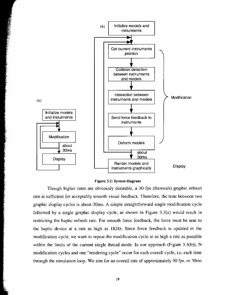
As shown in Figure 3.2(a), the simulator starts by initializing tissue and virtual

instruments models and then loops through a refresh cycle. Each refresh cycle consists of

as many modification cycles as can be executed in approximately 30 ms followed by a

single display cycle in which the updated tissue and instrument models are graphically

rendered. As shown in Figure 3.2(b), a modification cycle consists of updating the

instrument's current position, collision detection between instruments and tissue models,

determining corresponding interactions, deforming the tissue model and sending force

feedback to the instruments.

(h) p z E z i q insturments

Initialize models

Modification

about

Get current instruments position

between instruments and models

Interaction between instruments and models

Send force feedback to instruments

Deform models

about 30ms

Render models and

) Modification

Display

Figure 3.2: System diagram

Though higher rates are obviously desirable, a 30 fps (framesls) graphic refresh

rate is sufficient for acceptably smooth visual feedback. Therefore, the time between two

graphic display cycles is about 30ms. A simple straightforward single modification cycle

followed by a single graphic display cycle, as shown in Figure 3.3(a) would result in

restricting the haptic refresh rate. For smooth force feedback, the force must be sent to

the haptic device at a rate as high as 1KHz. Since force feedback is updated in the

modification cycle, we want to repeat the modification cycle at as high a rate as possible

within the limits of the current single thread mode. In our approach (Figure 3.3(b)), N

modification cycles and one "rendering cycle" occur for each overall cycle, i.e. each time

through the simulation loop. We aim for an overall rate of approximately 30 fps, or 30ms

per cycle. If T, Tm and Td are respectively the overall, modification and display cycle

times, then the number of modification cycles is N, where T = N* Tm + Td. The overall

rate of 1/T will vary with graphical complexity of the models and instruments, and with

CPU speed.

Traditional Single Thread rendering -

Modification cycle (Tm)

Display cycle (Td)

l- Modification

I cycle (Tm)

Display cycle (Td)

D

0

Improved rendering

-- 7

-Modification cycle (Tm)

-Modification cycle (Tm)

-Modification cycle (Tm)

Display cycle (Td)

N cycles*

T

* N cycles are defined to take * between 30ms and 30ms+Tm

Figure 3.3: System time distribution chart of rendering

In each modification cycle, the current position of every instrument is read in. For

each tissue model, we check for interference with all instruments. If interference occurs,

then the state of interaction is determined. For instance, if the force exerted by the scalpel

exceeds the cutting threshold, the tissue model will be cut, i.e. its topology will be

changed. The model will also deform due to the cut. Reaction forces will be calculated

according to the current interaction state and sent back to the haptic device. This process

is repeated for each instrument, as illustrated by the following pseudo code. We will

detail the different interaction state in chapter 5.

for (all the tissue model) {

for (all the instrument) {

Interference checking 0; Determine interactions 0 ; Modification according to interactions 0 ;

Calculate and send back force 0; 1 Model deformation 0 ;

1

3.2 Mass-spring Model To satisfy the requirement that objects must look and behave realistically, the

models must be based on physical laws governing the dynamic behaviour of deformable

objects. The choice between the two commonly used physics-based approaches, mass-

spring models and the finite element method (FEM), has long existed. Though the finite

element method offers more accurate modelling than mass-spring models, it is

computationally more demanding and usually requires considerable simplification for

real-time applications [PiciOO][NienOl][MorOO]. Furthermore, topology modification

precludes any pre-computation for FEM. Mass-spring models are widely used in

simulation of cutting due to their simplicity and low computational requirement

[Mese97] [BielOO] [BruyO 11.

In this section we will introduce our modelling method, a modified mass-spring

model. Such models are commonly used to simulate deformable tissue. In mass-spring

models, each vertex is a mass point (a node) and each edge is a spring and the edges form

a 3D mesh. Vertex displacements are calculated through solution of differential equations

that model the mass-spring system. As mentioned earlier, virtual objects can be modelled

by either volumetric element, such as tetrahedral or polygonal surface elements, such as

triangles. A mass-spring model can apply to both. However, calculating both vertex

displacements and topological modification is simpler for surface mesh models. In

addition, we are only interested in the outer surface for display. Therefore, we choose a

surface mass-spring model to simulate the deformable virtual objects in this thesis.

In our model, the simulated surface is divided into small triangles, where each

vertex is a mass point. A linear spring is defined along each triangle edge. These springs

are called "mesh springs" because they model the surface of the object. When a soft

elastic object deforms, the interior of the object also contributes to the shape of

deformation. To reflect this fact in our model, each node is also connected by a spring to

its initial or "un-deformed home" position, thus the name "home springs" (home position

and rest shape refer to the same configuration). Home springs can be used to define an

internal structure for the object. The set of home positions comprises the rigid kernel of

the deformable model, which preserves the object's shape [Mese97] [Zhan02]. We also

added damping to the mesh by adding to each mass node a force proportional to its

velocity, but in the opposite direction.

Figure 3.4: Part of a mass-spring model

Figure 3.4 shows part of the modelled surface. In this figure home springs are

drawn with nonzero length to depict their existence. Each edge can have a different

spring constant and the nodes can have different masses. However, the spring constants

are not based on real material properties as in FEM. For a homogeneous model, the

spring constant for each spring should be inversely proportional to spring length.

However, there is no well-accepted algorithm in the literature to set spring constants such

that the virtual mesh will have the same elasticity as real material. This mass-spring

model seems better suited for surgical training, which requires more emphasis on visual

realism than exact, patient-specific deformation, but requires that simulations be

performed in real-time.

Model deformation results in vertex displacement. The displacement propagates

to the neighbouring area due to spring forces. To simulate the tension of soft tissue, every

mesh spring has been initially stretched, i.e. its rest length is less than its initial length.

Thus, once a cut is made, surface spring forces will open up the cut.

3.3 Deformation Calculation At any time t , the motioddeformation of the mass-spring model M of n nodes i

(i=l, . . ., n) can be described by a system of n differential equations, each expressing the

motion of a node i:

22

x, = vi and Qi = a, = J; 1 mi (3.1)

In equation (3.1), xi and vi are the position vector and velocity vector; J; is the

total force (i.e., forces from other nodes and external forces, e.g. gravity force) exerted on

node i; mi is the mass value of node i, which is a scalar value. xi, vi , and f , are vectors

with three components, corresponding to the three coordinates in Cartesian space. Now,

in order to solve for xi in (3.1), we need a description of f , .

where 1, is the displacement vector from the node's current position to its home

position; l q is the vector pointing from the i th node to its j th directly connected

neighbour node; q, is the rest length of the mesh spring connecting the i th node and its

j th neighbour node; f;"s the external force applied on the i th node. We denote the

mesh spring constant as K , , the damping constant as K , , and the home spring constant

as K , .

This is a system of first order differential equations. We use numerical techniques

to approximate the solution. In our implementation, we use Euler's method for its

simplicity and efficiency as the following:

v, (t + At) = v, (t) + a, (t)At

xi (t + At) = xi (t) + vi (t)At (3.3)

The program starts with initial values of positions. The nodes start with zero

velocity. However, as we simulate the tension of soft tissue by initially stretching every

mesh spring, the total force on each node is not zero. Therefore, the nodes will move until

equilibrium positions are reached. This process takes only a few seconds depending on

the number of nodes and computing speed. The equilibrium positions are the actual start

positions of our virtual models.

There are two main approaches to calculate the deformation. One way is global

deformation, i.e. go through all the vertices in the model to get their equilibrium

positions. Another way is to use local deformation, in which the deformation calculation

is localized to a limited area around the affected area. Since time for a global deformation L* i x

calculation increasing linearly in the number of nodes in the mesh, the global deformation

is computationally demanding if the model has many nodes. If we only consider

deformations that start from a point of deflection instead of the area immediately

surround the cut, local deformation will significantly reduce the computational load. The

main idea of local deformation calculation is that if the total force f , on a vertex is

smaller than a threshold, propagation of the deformation calculation will stop [BrowOl].

We start the calculation from seed vertices, which are the three vertices of the intersected

triangle, as the three circled nodes shown in Figure 3.5. We calculate the deformation of

each seed vertex; if the total force is bigger than the threshold; we then traverse to their

neighbour vertices. Neighbour vertices are the vertices directly connected to this vertex

by an edge, as shown in Figure 3.5.

Figure 3.5: Illustration of local deformation calculation propagation.

3.4 Collision Detection The collision detection procedure detects any interaction between the surgical

instrument, such as scalpel, grasper and cautery hook, and the virtual tissue model.

Surgical instruments have different shapes and functionalities (Table 3.1). As a result,

different rendering and collision detection algorithms are needed for determining the state

of interaction between the tool and the surface.

Real Instrument

Picture

Virtual Instrument Collision Detection

Representation

Table 3.1: Surgical instruments

As shown in Table 3.1, we have simulated two instruments used in laparoscopic

surgery, a grasping forceps (referred to as grasper in this thesis) and a cautery L-hook.

We also simulate a scalpel that is widely used in open surgery. For the purpose of

graphical display, instruments are represented by many triangles in order to give the

instrument a realistic appearance. The third column in Table 3.1 is screenshots of our

virtual instruments in the simulator. For collision detection purposes, the instrument

representation is simplified to a small set of line segments, as shown in the forth column

of Table 3.1. Collision detection then reduces to detecting intersections between line

segments and triangles (See Appendix B for detail algorithm). We will find the exact

intersection point of the line segment and triangle. We define two types of line

corresponding to different portions of the instruments. One type of line deforms the tissue

when it contacts the tissue. The other type cuts the tissue. As shown in row 3 column 4,

AB and BC are the cutting lines for cautery hook while CD deforms. All the lines of the

grasper deform the tissue by either pushing in or stretching out. For the scalpel, we only

consider line segment AB as the sharp edge, which represents the blade, and all the other

line segments deform. Therefore, the collision detection method for different instruments

varies.

Chapter 4

4 Progressive Cutting

Tissue dissection is an important procedure in surgical simulation systems.

Dissection involves cutting through and separating tissue after a cut. Users of surgical

simulators expect to see the result of cutting as they move the instrument, without

noticeable delay. Re-meshing is needed for this and must be performed as the cutting tool

travels along its path. This is referred to as progressive cutting, and excludes algorithms

that depend on knowing the final intersection state of the instrument and the virtual

models. Mor and Kanade [MorOO] first detailed a method to modify tetrahedral elements

simultaneously with tool movement.

We propose a surface subdivision method to generate a progressive cut as the

cutting instrument moves within a triangle. We have not found any previous detail

description of similar work in the literature. The subdivision scheme applied to each

triangle is determined by the state of intersection with the instrument. A state machine is

introduced to model two types of progressive cutting.

In our proposed method for dissecting an object and splitting it into many pieces,

the original un-cut model is separated at the data structure level, which represents the

object. In this approach, each dissected piece can subsequently be manipulated

individually, i.e. it can be deformed, moved away by a grasping tool, or further dissected

into smaller pieces. It is believed that such a modelling approach offers an important

advance in surgical or biological simulators.

In this chapter, we describe our progressive cutting algorithm, which simulates

the tissue dissection operation based on a surface mesh model. Following the introduction

of some useful notation, we introduce our generalized progressive cutting and interior

structure generation algorithms. Our method to completely divide a model into two

components, i.e. dissect it, and move one or both components will also be described. We

will also present some results from our system along with a brief performance analysis.

Finally, a discussion of the approach and suggestions for future work are given.

4.1 Conceptual Overview 4.1.1 Definitions of cut

In our simulation, a cutting operation is defined as the movement of a cutting

instrument while penetrating an object. To speed up collision detection computations, we

simplify the cutting instrument and represent it as one or a small number of line

segments, representing cutting edges,. Collision detection then reduces to detecting

intersections between line segments and triangles.

Figure 4.1: Example of cutting operation

Figure 4.1 shows an example of part of an object surface model composed of

triangles. A cutting path is defined by moving a virtual instrument through the mesh.

Once the instrument makes contact with the object, e.g. triangle TI , we deem it as the

start of a cut. As the instrument moves, the underlying object mesh is modified by local

subdivision. This subdivision algorithm will be described in Section 3.2. Depending on

the relative sizes of the mesh and the instrument, the instrument path inside a triangle

may not be a straight line, e.g. the dashed line in Figure 4.1; however, we simplify any

path within a triangle to a single straight line segment connecting the first and last (or

most recent) intersection points in the triangle (solid line). If the instrument is lifted up

and loses contact with the object, the algorithm enters a termination state. For example,

triangle T7 is the last triangle that the instrument has contacted. In this thesis, triangles

like T1 are called start state triangles and T7 are called termination state triangles,

T2.. .T6 are referred to as midway triangles.

4.1.2 Side of the blade the vertex is on When the path crosses a triangle's edge, we generate two new vertices on that

edge by subdivision. One will lie to the left of the blade and one to the right. When the

path goes through a vertex, the vertex will be split into two and triangles around that

vertex must be reconstructed. In order to properly subdivide the triangle it will be

necessary to know which side of the "blade" each vertex of the cut triangle is on. We use

the scalpel-edge sweep plane to determine this, as shown below. We set a flag for each

vertex, called a side flag, for later use.

Figure 4.2: Finding which sides of the blade plane vertices are on.

As shown in Figure 4.2, P,urre,, is the current intersection point and PpreYiouS is the

previous intersection point.

Define vector path = P, ,,,,,, - P p,,v ious

Since the previous scalpel direction and current direction may not lie in the same

plane, the scalpel sweep plane is defined as a plane containing the path vector and the

current scalpel axis. This plane then determines which side of the blade vertices A and C

are on. Looking at where the scalpel came from, A is to the left and C is to the right in

this example. However, choosing which is left (and right) is not critical to the system; we

just need a consistent reference.

4.1.3 Two types of cutting With our surface mesh model, we consider two types of cutting in our simulation.

As shown in Figure 4.3(a), we say a "cut-into7' type of cutting occurs if the instrument

only penetrates one layer (also referred as the top layer in later descriptions) and

"groove" triangles will be generated. "Cut-through" type cutting occurs when the

instrument cuts completely through the object (both the top and bottom layers). Triangles,

referred to as "side" triangles, which connect top and bottom layers will be created

depending on the type of intersection.

Figure 4.3: Illustration of two types cutting

4.1.4 Two ways to start a cut For general dissection operations, we must deal with the cutting instrument

starting to intersect the object in two different ways. Figure 4.4 illustrates possible state

changes between the intersection cases of the cutting instrument and object. "Pierce-in"

occurs when the instrument's tip penetrates the object first, like cut-into; the instrument is

moved essentially along its long axis. However, if the instrument continues pushing

through the object, entering by being moved perpendicularly to its cutting edge, it

penetrates two layers, generating a cut-through type of cut. Figure 4.1 is an example of

pierce-in. The second case is called "slide-in" and occurs when the cutting edge of the

instrument cuts into the tissue while its tip is outside of the model. Here, the line segment

representing the sharp edge of the instrument has, in general, two intersections with the

model surface. In this case, the start state triangles on top and bottom layers must be

adjacent, i.e. share either an edge or a vertex.

Figure 4.4: Intersection state machine.

If the instrument pierces the top layer only, it "cuts-into"; the state is "cut-

through" if it cuts completely through the object. The state may change as the instrument

cuts, depending on depth of cut

If the cutting tool slides-in and cuts-through the whole object, the object is

dissected into two pieces. We also propose a method to separate the model into two,

described in section 4.3.

4.2 Collision Detection To find the first cutting point, all surface triangles are tested for intersection with

the sharp edge. The exact intersection point of the instrument and the tissue model is

found by a line segment, i.e. the sharp edge, and triangle intersection algorithm. For

detail of this algorithm, please refer to Appendix B. All the mesh triangles are stored in a

list. We go through this list with line-segment triangle intersection checking until we find

an intersection point. This global search is time-consuming if the model is complex.

However, since neither further calculation nor haptic feedback is needed if no

intersection is found, a global search is acceptable at this stage.

When we find the first intersection point of a cutting edge and the tissue surface,

the next step is to decide whether the cutting threshold is exceeded. This threshold

represents the border between deformation and cutting. The value of the threshold can be

tuned experimentally based on real material properties. In our simulation model, the

threshold is currently applied to the amount of force exerted on the object surface by the

instrument. When the force exerted on the object by the instrument is not sufficiently

large to tear open the surface, a deform state exists, and the instrument deforms the

object. When the cutting instrument has penetrated the object surface, and cutting is

allowed, a cutting state exists. A special case of interaction is the use of the blunt edge of

the blade surface of the scalpel as a probe. Here the model deforms rather than being cut.

We will describe these interaction states between scalpel and tissue model further in

Chapter 5.

After detection of the first cutting point, we still need to search globally, testing

all other triangles to see if cut-through has occurred. If so, we will have two intersection

point sequences, one for the top layer and the other for the bottom layer. The collision

detection search sequence is the same for each layer.

Figure 4.5: Example of triangle adjacency

32

Triangles sharing an edge with the current triangle are "edge neighbour" triangles

to the current triangle, e.g. EN1-EN3 in Figure 4.5. If the cutting tool moves into the

current triangle's edge neighbour triangle, the cutting tool goes across that common edge.

Other triangles, which only share a common vertex with the current triangle, are called

"vertex neighbour" triangles, e.g. VNI-VN9 in Figure 4.5. Usually the cutting tool does

not go across a vertex exactly; if the cutting tool does go into a vertex neighbour triangle

we deem the scalpel to cross the vertex shared by these two triangles.

Since in a medical context, all motions of the tools are slow (and with limited

jitter),, movements of the instruments are assumed to be continuous and smooth so

collision detection can be continued locally with neighbouring triangles of the currently

intersected triangle. How the cutting tool goes into or out of a triangle, i.e. by an edge or

vertex, will change the subdivision state applied to the triangle.

4.3 Progressive Cutting and Interior Structure Generation

For a surgical training environment, the user expects immediate visual and haptic

feedback while the cut is in progress, and a simulator that supports progressive cutting is

needed. We have developed a method of progressive cutting, which splits triangles while

following cutting instrument motion. The interior structure is also generated in a

progressive way. Texture mapping of the generated interior structures provides further

realism.

The main idea of progressive cutting is to temporarily subdivide the triangle

intersecting the instrument, making use of a state machine. Table 4.1 shows our surface

triangle progressive subdivision state machine.

Table 4.1: Surface Triangle Progressive Subdivision State Machine

State Change ....................

Start State

Termination State

Midway State

kt-through Edge ht-through Vertex

When the scalpel enters a triangle, it will be subdivided according to its state. The

intersected triangle is deleted, leaving a hole. New smaller triangles are then generated,

and form a local mesh, which is merged into the overall mesh as a "patch". To save time,

the deleted triangle is actually deleted from the mesh's triangle list only when a cut is

completely finished. A permanent subdivision state is entered when the instrument moves

out of that triangle. Subdivision adds new vertices to the model as mass points, and edges

as springs.

4.3.1 Surface subdivision algorithms

Start state triangle

The first intersected triangle, referred to as the start state triangle, will not be

subdivided until the scalpel exits this triangle. We define two subdivision templates for

the start state triangle, as shown in Figure 4.6; one when the scalpel exits via an edge

(SE), the other one via a vertex (SV).

Figure 4.6: Start state triangle subdivision templates

If the scalpel exits via an edge (edge BC in SE), triangle ABC will be subdivided

into four small triangles. Newly generated vertices E and F are coincident where the cut

intersects edge BC and are connected to the object surface by springs along the edges of

the triangle. Home positions of the newly generated vertices are set to their initial

positions when they are created. Spring forces, obtained through solution of the new

mesh equations, will move E and F apart. Vertices on the surface like D, E and F in this

case, will be connected to groove or bottom vertices to form the interior structure of the

cut. Groove or bottom vertices are generated when we subdivide the surface triangle. We

will explain how we create groove or bottom vertices in later section.

When the scalpel passes a vertex (SV), the vertex C will be split by creating two

new vertices (E and F) at the position of C. Then vertex C is deleted and all the triangles

around it are regenerated using the new vertices.

Termination state triangle

If the instrument is retracted from the cut and contact with the object is lost, we

deem this cutting operation terminated. When the scalpel enters a triangle, except at the

start state, we always consider that triangle (initially) as the termination state triangle, i.e.

it is the last intersected triangle of this cut. The triangle is subdivided temporarily

according to the current intersection state. If the instrument moves within triangle ABC

(Figure 4.7, TE), the current topology is maintained and the temporary elements are

updated using the new instrument position, which results in the new positions D and D'

We use two separate vertices here in order to simplify later subdivision changes. D and

D' are bound together when the scalpel is still inside current triangle. Users thus see

immediately the result of their operation. By this means we accomplish progressive

cutting. We also have two cases of "termination state" (Figure 4.7).

Figure 4.7: Termination state triangle subdivision templates

Midway state triangle

As the scalpel exits the temporary termination state triangle and moves into an

adjacent triangle, the triangle just left enters a midway state. The triangle's topology will

be changed depending on exactly how the instrument enters and exits. The midway state

is formed by simply deleting one or two of the small triangles newly generated in the

previous temporary termination state. Since no vertex is deleted by this means, there is no

need to modify groove triangles or side triangles (as defined in section 4.1.3 and Figure

4.10). Figure 4.8 shows two examples of midway subdivision templates. MEEl is the

case where the instrument enters and exits (cuts in and out) a triangle via two different

edges. MVEl is the case where the instrument cuts in from a vertex and cuts out from an

edge. We have developed a total of 8 templates covering all possible cases as shown in

Table 4.1.

Figure 4.8: Examples of midway state triangle subdivision templates

We show two examples of the state changes of progressive cutting in Figure 4.9.

In the left image, triangle ABC is the start state triangle, subdivided using SE since the

scalpel exits via edge BC. Triangle BCD is temporarily subdivided as a termination state

using template TE. In the right image, the scalpel continues cutting. Triangle BCD

changes to a midway triangle and is subdivided using MEEl since the scalpel cuts out

from edge CD. Triangle CDE is temporarily subdivided as a termination state.

Figure 4.9: Example of progressive cutting. (a) Scalpel cuts out from edge BC to triangle BCD. (b) Scalpel cuts out from edge CD.

4.3.2 Groove and side triangle generation Since the object is simulated by a surface mesh, the inside of a cut is not

represented, i.e. it appears empty. We have developed a method to generate structures in

the opening as a function of the depth of the instrument penetration, see Figure 4.10. For

cut-into, we use the instrument tip positions at the start and end of the cut inside one

surface triangle to define the bottom of a groove (B1 and B2 in Figure 4.10(a)). Surface

vertices generated by subdivision are SLl and SL2 (left side of the cut) and SRl and SR2

(right side) respectively. Left and right sides are defined looking at the direction of

scalpel motion. When the scalpel cuts through the whole object, as shown in Figure 4.10

(b), the bottom layer surface is also subdivided using the templates we just described.

Figure 4.10: Groove (a) and side (b) triangle generation

We have developed a single algorithm to generate new surfaces in the opening for

both cases. We keep four arrays of pointers to the unconnected vertices, called

SurfaceRight, SurfaceLeft, BottomRight and BottornLeft. Cut-into, BottomRight and

BottomLeft actually point to the same vertex. Using this scheme, we can use a common

algorithm to deal with both cases. The subdivision templates used for the top layer and

bottom layer can be different since we do not require the structure of the two layers to be

identical. Therefore, the number of unconnected surface and bottom (groove or bottom

surface) vertices need not be equal.

Figure 4.11 shows an example of connecting part of the right side vertices to form

side triangles. Left side is dealt the same way. Every time a surface triangle is subdivided,

whether top or bottom layer, we try to generate new triangles by connecting newly

generated vertices with the last unconnected vertices on the other layer. In this example,

the top layer has three newly generated vertices while the bottom layer has four new

vertices need to be connected to form side triangles. We first create triangles SR1SR2BR1

and SR2SR3BR1 by connecting vertices SR1, SR2 and SR3 with bottom vertex BR1. Then

we generate triangles BR1BR2SR3, BR2BR3SR3 and BR3BR4SR3 by connecting bottom

vertices with top vertex SR3. The algorithm can also be explained as the following pseudo

code, as shown in Figure 4.12.

Figure 4.11: Side triangles generation algorithm

GenerateTriangles(vector<vertex*> top, vector<vertex*> bottom) {

for (i=O to top-size-1) FormTriangle(top[il,top[i+ll,bottom[0]);

Temp = top-last; top-clear ( ) ;

top[OI =temp;

for (i=O to bottom.size-1) FormTriangle(bottom [i],bottom[i+l],top[O]);

Temp=top.last; top. clear ( ) ; top[OI =temp;

1

Figure 4.12: Psudo code for generating side triangles

4.3.3 Object Boundary Condition Case Since the tissue model can be any 3D shape and the cutting instrument can come

from any direction, there is no clearly defined geometric boundary of the model. As

described in the slide-in case, if the top and bottom layer intersected triangles are

adjacent, i.e. they share an edge or vertex; we define these two triangles as the boundary

of the current cut. The boundary triangles can be either start state, referred to as "cut-in",

or termination state, "cut-out". Figure 4.13 shows an illustration of a "cut-out" case:

Top layer

\ I Sharp Edge

Figure 4.13: Cut-out from a common edge

In Figure 4.13(a), we show an example of boundary triangles sharing a common

edge. Once we detect that top and bottom layer intersected triangles share an edge, for

example triangle ABC and BDC share edge BC in Figure 4.13, we assume the tool will

cut out at that edge. Due to the finite sampling rate, the last intersection point we find

may not be exactly on the common edge. However, we assume that in general the

boundary triangles are small and this approximation can be acceptable for a training

environment. Figure 4.13 (b) shows a subdivision result. The algorithm for cut-in is

similar to that for cut-out.

Figure 4.14: Example of cut-in from boundary

Figure 4.14 shows a wire frame cut-in example of the boundary of a thin circular

plate where, after sliding-in, the scalpel cuts through the model.

4.4 Separation When the cutting instrument pierces the object, we actually add new geometry

primitives (triangles, edges and vertices) to simulate the visual results of the area, which

is newly exposed due to the cut. We still only have one mesh for the object. However, if

the object has been completely cut, the object should be separated into two pieces. The

subdivision and interior structure generation algorithms generate new primitives, which

are appended to the original mesh (Figure 4.15). Though these new primitives make the

original object appear as two parts, it is still one mesh at the data structure level. All

vertices, edges and triangles are still stored as a single mesh, though there is no

topological connection between the two parts.

We developed an algorithm to create a new mesh (and a new object

corresponding to it) composed of triangles from the cut off part, and separate it from the

original mesh. We arbitrarily define the right part (defined looking in the direction of

scalpel motion) as the new part. After the object has been completely cut-through, we

determine which triangles belong to the new mesh. Every triangle has a flag showing

whether it is still belong to current mesh. Initially, the flag is "0" for all the triangles in

the mesh. As shown in Figure 4.15, we start the labelling process with the last created

triangle (it belongs to the right side according to our algorithm) to find all of its edge

neighbour triangles. After labelling these triangles we visit their neighbour triangles and

repeat iteratively until no more neighbour triangles are unlabeled. We also label all

vertices and edges belonging to these triangles in order to distinguish primitives

belonging to the new part. The final step is to remove these primitives from the original

mesh triangles list and use them to create a new mesh. The new mesh can then be dealt

with in the same way as the original mesh for collision detection, cutting subdivision, etc.

1 M e MI 1 Mesh after cut, new triangles have been added

Separate the triangles and create new mesh. Change the flag to "On after the new mesh has been created

- ,Triangle --------------- riangle riangle - 2 -

1

Label the triangles, if the triangle needs to be separated from Mesh 0 current mesh, change the flag to "1"

Mesh 0 Mesh 1

Triangle V 1 - n

Triangle 0

Figure 4.15: Data structures involved in creating a new mesh

L , V - - -

- Triangle 7

0 - - -

4.5 Results and Performance Analysis

Triangle 1

Dissection methods described in this paper have been implemented and integrated

--------------- riangle riangle .-+Triangle 2

into our prototype surgical training environment. Currently the system is running on a PC

- % - - -

with an Intel 2.8GHz CPU and 1GB of memory, under Windows XP. Both a haptic

feedback device (Immersion Laparoscopic Impulse Engine) and a non-haptic device

(two-handled Immersion Virtual Laparoscopic Interface) have been integrated into the

system (Figure 4.16)

Figure 4.16: Setup using two-handled input device

42

Figure 4.17 gives a closer look at a thin circular plate manipulated by the two-

handled device (Figure 4.16). The virtual scalpel has dissected the object and the newly

created part has been rendered in wire frame mode while the remaining part of the

original object is moved away by a grasper. The initial model had 720 triangles. The

update rate was about 1400Hz, which, for this relatively simple model, certainly meets

the lOOOHz smooth haptic rendering requirement.

Figure 4.17: Dissecting an object; new mesh generated by separation method is rendered in wire frame while the remaining portion of the original part is moved away by a grasper.

Figure 4.18 (b, c and d) show 3 frames of a sequence representing a progressive

cut of a liver model, initially composed of 2466 triangles. The update rate here is about

330Hz. Figure 4.18 (e) illustrates the mesh topology of our model after the cut. The

groove triangles are rendered as a red surface while the outside surface is rendered in

wire frame mode. Figure 4.18 (f) shows multiple cuts-into in a single model.

(a) Setup with haptic feedback device (b) Start of the cut

43

(c) Cut in progress (d) Finished cut

(e) Wire frame after one cut (f) Three cross cuts

Figure 4.18: Progressive cut of liver model with haptic feedback device

Figure 4.19(a) shows an example of dissecting a cylindrical shape. It shows our

algorithm's ability to deal with general shapes, regardless of the degree of local curvature

with respect to a cutting tool. We first slide in and cut completely through the cylinder.

Once the scalpel exits the cylinder, the model is separated in two, i.e. a new model is

generated for the right portion of the cylinder. We then work on the newly generated

model with examples of "cut-into" and "cut-through" processes. Finally, the model is

dissected once more and a virtual grasper manipulates portions individually (Figure 4.19-

b).

Figure 4.19: Dissect the cylindrical shape model into pieces and manipulate the middle part away by a grasper.

Table 4.2 shows an example of our system performance for a surface model,

which initially had 7200 triangles. The first column is the cumulative number of triangles

that have been cut for a given iteration; the second shows the cumulative number of

triangles added to the model, including groove triangles. The third column reports the

average time to perform one loop while cutting. The average number of new triangles

added to the mesh due to subdivision and creation of groove triangles is about six for

each intersected triangle, which is as good as the "minimal new element creation"

reported in [MorOO].

# of triangles cut # of triangles Loop time during added cutting (ms)

0 0 10.3 2 14 7.7

20 122 8 .o 100 560 9.1

Table 4.2: Cutting algorithm performance example

Table 4.3 gives detailed data on our system performance for a surface mesh model

which initially had 14,400 triangles and 7200 vertices. It provides a further description of

the time to update object deformation, collision detection between instruments and

object, re-mesh the model to simulate the cut by subdivision, and the calculation of

vertices' normal after deformation. We calculate the new (deformed) position of every

vertex by solving the differential equations of the mass-spring model. The number of new

vertices that have been added to the mesh is listed in the third column. Since the number

of vertices did not increase dramatically due to the cut, the time to update the position of

each vertex does not increase much. As we mentioned in section 4.2, we search all

surface triangles for an intersection point with the cutting instrument to find the first

intersection point. Once we find the first intersection point, we only search in the

neighbourhood of the current intersection. Therefore, the collision detection time before

the first cut is much longer than later local detection. The data shown in the sixth column

indicate our surface triangle subdivision and interior surface generation algorithms are

quite efficient. For graphic display, when we apply Phong shading to shade the object's

surface, vertex normals are pre-calculated for each vertex and stored together with the

rest of the object's data. When the object is deformed, the surface changes significantly

and vertex normal must be recalculated as part of the update sequence which, as the last

column shows, is time consuming.

# of # # Deformation Collision Remesh Calculate triangles triangles vertices Time (ms) detection Time Normal

cut added added (ms) (ms) (ms>

Table 4.3: Detail system performance data (Model initially has 14,400 triangles and 7200 vertices)

4.6 Discussion To simulate progressive cutting of a deformable object we have extended the

surface mesh model such that the interior structure of a cut is modelled and can be

visualized. The method to subdivide the surface mesh and generate grooves and side

topology is novel and efficient compared to the widely utilized volumetric model. We

also proposed a method to separate the model after cutting and create a new mesh object

for the part cut off, which extends the simulation of cutting to the more general

simulation of dissection. We have not been able to find any detailed description of this in

the literature. The surface mesh model we proposed makes dissection much easier and

simpler than using a tetrahedral model. Our algorithm's performance on a relatively

inexpensive PC is better than the data reported in the references [Bruy02].

However, there are also some limitations with our cutting algorithm. First

problem lies in correctly handling certain cases when the scalpel slides-in, i.e. it moves

into the tissue while its tip remains outside the model. Here, the line segment representing

the sharp edge of the instrument has two intersections with the model surface. In this

case, we require the start state triangles on top and bottom layers to be adjacent, i.e. share

an edge or a vertex. However, it is possible for the virtual cutting tool to miss the first

encountered triangles due to sampling latency, i.e. the two start state triangles on top and

bottom layers found by the program are not adjacent. This problem may also occur if the

curvature where the cutting tool slides in is large, i.e. a triangle may be almost parallel to

the cutting edge. Thus it is possible for the algorithm to miss such intersections. This

problem also occurs in the "cut-out" boundary case. To address this problem, we linearly

interpolate between the previous and current cutting edge positions to find possible

missing intersections. These added interpolated edges increase the possibility to detect

the "slide-in" case. We also require the movement of the cutting instrument be slow and

smooth at the object boundary area.

A second issue is that our collision detection algorithm only checks two layers for

intersections between cutting instrument and object surface. Therefore, it cannot handle

cases where the instrument has more than two intersections with the object surface.

Figure 4.20: Example of multiple (more than 2) intersection points on the object surface. (a) and (b) single object examples (c) multiple objects cut simultaneously by single instrument.

As shown in Figure 4.20, our current algorithm cannot handle a single object with

more than two intersection points with the cutting instrument (Figure 4.17 (a) and (b)).

However, our progressive cutting algorithm can simulate simultaneous cuts on multiple

objects. Therefore, if we can alter the model that we are trying to cut to that of Figure

4.20(c), the method we developed can work well.

As pointed out by [NienOl], subdivision methods increase the number of triangles

in a mesh, which may increase the calculation load of the relaxation. They may also

produce tiny triangles, which are problematic for intersection testing. Therefore, it is hard

to continue a cut from the exact position where the previous cut stops. Tiny triangles may

also cause the mass-spring system to become unstable. Our home spring helps to make

our enhanced mass-spring model more stable. A method to remove tiny triangles after

subdivision is needed.

These issues can be addressed in future work.

Chapter 5

5 Tissue Interaction and Haptic Feedback

We have implemented support for three surgical instrument models for this thesis

work: scalpel, grasper and cautery hook (see Table 3.1). The interaction between these

instruments and the virtual tissue model can be categorized as deforming, cutting, and

moving. All three instruments can deform the tissue. Different instruments will deform

the model in different ways and we will detail the interactions in later sections. Scalpels

and cautery hooks can also perform cutting actions as we have explained in chapter 4.

Graspers can grasp tissue, either to hold it out of the way or to remove tissue fragments

from the surgical field. Cutting will modify the topological structure of the tissue model.

Deforming and moving will not change the underlying structure.

Haptic feedback can offer a natural sensation similar to what a surgeon might feel

in performing the actual surgery. Therefore, it is an important aspect of surgical

simulators. Our current system uses an Immersion Laparoscopic Impulse Engine (LapIE),

which is kinematically similar to the tools used in laparoscopic surgery, as shown in

Figure 5.1. This device provides haptic feedback to the user as they interact with virtual

objects. Reaction forces generated during a cut are computed and sent to the haptic

device.

Figure 5.1: Immersion Laparoscopic Impulse Engine (LapIE). Reproduced by permission of Immersion Corporation, Copyright O 2004 Immersion Corporation. All rights reserved.

We will explain how we simulate these interactions and the haptic feedback

models we proposed for these interactions in this chapter.

5.1 Depressing Tissue While cutting is the main method surgeons use to modify and change tissue, it is

not the only way that surgeons interact with the surgical site. Palpation is used quite often

to determine possible pathologies in tissue and the location of particular features

[MorOl]. Palpation can be viewed as a method of applying external force to an object,

either using the fingers directly in open surgery or through some instrument in minimally

invasive surgery. Here we only consider the minimally invasive surgery case, i.e. using

instrument to deform the tissue. We refer to palpation deformation as depressing in the

later description. All the instruments can deform the virtual tissue model.

In this section, we first explain how we simulate the deformation and the resultant

reaction forces with the proposed tissue model. By depressing, we mean altering the

tissue shape by stress. When the instrument presses the tissue surface and deforms it, the

intersected area is moved down accordingly. If the tip of the instrument is blunt (or the

cutting threshold has not been reached), the tissue surface will not be broken and

penetrated, and, the instrument remains outside the surface. For simplification, we only

consider interaction between the instrument tip and the tissue model. Figure 5.2 shows a

picture of depressing real tissue.

Figure 5.2: Real picture of deforming a tissue via depressing it.

When a user deforms tissue with an instrument, he/she exerts a force Fex, on the

tissue. The tissue resists this deformation depending on its internal structure and material

properties, and responds with a reaction force F,,,,, . As long as I F,, ( > ( F,,,,, 1, the tissue

is deforming, i.e. the tissue surface goes down and down. When the two forces have the

same magnitude but in opposite directions, an equilibrium state is reached and the

deformation does not go any further. The force sent back to the user is equal to F;,ss,, at

equilibrium. If Fext is smaller than F;,,,, , the tissue moves back toward its initial position.

Since our tissue is modelled by a network of mass nodes, part of the mass-spring model,

the external force F,, exerted by the user is applied to these mass nodes. However, most

force feedback devices, including the LapIE we used, cannot sense the forces applied by

the user directly. Only position information is available from the device. Usually the

external force F,, used in the deformation calculation is an approximation instead. One

common way is the penalty-based method, i.e. a virtual linear spring is placed between

the current instrument tip position qiP and an appropriate reference point P,f and the

spring force F, is used as the approximation, F,,rt = -F,, = c*(eip -P,,f) [Biel03]. This

approach is not very realistic since the instrument tip vanishes inside the tissue during the

deformation. Also, it is hard to determine an appropriate constant c to reflect the tissue

stiffness and define a suitable reference point.

We have proposed a simple method to simulate the deformation by assuming at

any time step during the deformation, it is at an equilibrium state, i.e. the instrument tip is

always outside of the tissue surface. We achieve this by simply pushing the intersected

triangle down. As shown in Figure 5.3, when the instrument intersects surface triangle

ABC, we simply move triangle ABC by the vector from the intersection point to the

current probe tip position, 7 = as if the instrument displaced the whole triangle

down as a plane, as shown in Figure 5.3. Triangle ABC's neighbours will then deform

because of the connecting springs.

Figure 5.3: Tissue surface deformation model, close look

In this approach, we approximate the force applied by the user, F,, , by calculating

the restoring force F,,,s,, , resulting from the surface mesh deformation caused by the

instrument. For each vertex, the spring force can be expressed as:

where k,, and 1, are the spring constant and displacement vector of the home

spring, k, is the mesh spring constant, /,is the vector pointing to the jth mesh spring

connected to this vertex, rm, is the rest length of that spring and the summation (j) is over

all springs connected to that vertex. The deformation force is then:

and increases as the instrument goes deeper.

This force feedback model also works when the instrument slides over the soft

object surface while deforming it. However, in this case, a dynamic friction force should

be added. We set the friction in the deformation state to be proportional to velocity and

the magnitude of the tissue reaction force F,,,,, .

where Vs,,lp,l is the tip velocity direction. The total force sent back to the haptic

device in this case is:

- Fdeform--feedback - c i s sue + Fdeforrn- friction

5.2 Interaction between scalpel and model Our virtual scalpel can deform and cut the tissue model. In contrast to real cutting,

virtual instruments can move in any direction unless appropriate constraint forces are

applied. Obviously, real instruments used during real surgery have constraints on the

directions in which they can move. For example, a scalpel has only one cutting edge, and

thus cuts only in the direction of its blade. To provide such a constraint in a virtual

environment, we implemented a haptic feedback method.

We constrain scalpel motion to be in the direction of the blade. Scalpel motion in

one time step is (Figure 5.4), with components in the cutting direction,

&perpendicular to the previous blade plane and ;i6 in depth. If I d / I d, 1 is greater than

a certain value S , we deem the scalpel to have moved sideways. In this case, a

deformation, referred to as sideways deformation, occurs instead of cutting. However, if a

device without haptic feedback is used, the virtual instrument can move in any direction.

The tissue model is still deformed but no force feedback is sent to constrain the

movement.

Figure 5.4: Decomposition of scalpel movement

5 3

However, if we overly constrain the motion, the scalpel can only cut in a straight-

line path, while in reality curved cuts are certainly possible. By checking scalpel motion

using the scalpel tip as the monitored point, our simulator allows the user to make slow

changes to the cutting direction. We use the blade plane as a reference of the "correct"

path plane. The reference plane remains unchanged if the scalpel moves sideways.

Otherwise the current blade plane is set as the reference blade plane to allow slow turning

of the scalpel. We can choose a higher value of S to allow quicker turning of the scalpel.

We calculate the distance of the scalpel tip to the reference plane for the sideway

movement. If the distance decreases to less than a deviation threshold, we consider the

scalpel has returned to the "correct" path.

The flowchart of our scalpel-tissue interaction model is depicted as Figure 5.5. If

the scalpel first intersects a groove triangle generated by a previous cut, we need to

determine its direction of motion. If it is a sideways motion, the scalpel pushes the groove

surface sideways. This is a special case of interest where the flat side of the scalpel blade

surface is used as a probe. Here the model deforms sideways. At the next intersection

point (i.e. intersection point at next time step), we will check whether it returns to the

"correct" path: if so, a cutting action occurs; if not sideways deformation continues.

Find first + AX sideway?

Yes L

deform

ntersect? -3 utting plane? e

threshold? I Press deform 6

Get next

intersect? + Figure 5.5: Flowchart of scalpel-tissue interaction

If the first intersection was not on a groove triangle, the scalpel can deform the

tissue model if the cutting threshold is not reached. This is a depress state, simulated by

the method we just described. However, the principal function of the scalpel is cutting,

described in chapter 4. When the cutting threshold is reached, the scalpel penetrates the

surface and a cutting state is entered. Scalpel motion cuts the tissue, with the ongoing cut

modelled by progressive subdivision as described in chapter 4. The cutting state can still

change to sideways deformation if the scalpel moves sideways.

To constrain sideways motion, we define a constraint force Fron.rrrajnr in the

direction of d , . Fconsrrnjnr is proportional to the distance of the scalpel tip from the

reference blade plane. Figure 5.6 shows a sample screen image, in which the model has

already been cut; the scalpel is pushing the groove surface to the left and is deforming it.

A constraint force Fron,r,jnr is sent back to the device as haptic feedback.

Figure 5.6: Image of scalpel moves sideway inside a previous cut groove.

In our cutting force feedback model, we approximate the force conveyed to the

user with three components. Even if during the cutting action, the scalpel moves

sideways, all three components are sent back to the user since the cutting state has

already been entered.

Fre,,, is along the instrument's axis, countering further penetration and is

proportional to the penetration depth. We try to make it be large enough to prevent the

whole blade and shaft from entering the object.

where cwis, is the spring constant for a virtual spring connecting the bottom point

6 o t t o m (scalpel tip for the cut-into case and the bottom layer intersection point for the

cut-through case) and eOP, the intersection point on the top layer, as shown in Figure 5.7.

Note that both P,o,o,,, and eoP are updated at each time step.

Figure 5.7: Illustration of calculating resistant force for two cutting cases

While cutting, the friction force is proportional to the contact surface area

between the scalpel blade and the groove or side surface. However, since the groove and

side surfaces are also generated progressively, we approximate this with a simple model:

where is the penetration of the blade.

5.3 Interaction between grasper and model Grasping and moving is another common interaction in surgery. It is used for

many different purposes, such as to remove tissue fragments from the surgical site, to

hold the tissue and keep it away from the surgical site, and to stretch the tissue to expose

a cut surface. A grasper can be used to palpate tissue when nothing is being grasped. If

part of the tissue has been grasped, the grasper can either stretch to deform the tissue or

move the tissue fragment completely away.

Figure 5.8 shows an example of using the grasper to grasp and stretch a tissue in

real surgery. We can see the tissue is deformed when it is grasped.

Figure 5.8: Example of grasping and stretching the tissue by a grasper in real surgery

57

The interaction of the grasper is determined by the angle between its two jaws. As

shown in Table 3.1, line segments AC and BC represent the two jaws of the grasper. We

say the grasper is closing when both of the following conditions are met:

The angle between the two jaws decreased from previous angle;

The angle is also greater than a threshold angle, which is considered as closed.

Figure 5.9: Illustration of grasper jaw collision detection

When the grasper comes to interact with the tissue model, if the two jaws are open

or it is totally closed, it will deform the model. We use a two-level approach to find the

intersection points of the grasper and the tissue model surface. First, we use a

computationally inexpensive method, bounding box, to find potential intersection

triangles. We then use a line-triangle intersection method to find the exact collision point.

As shown in Figure 5.9, when the grasper starts to interact with the model with its jaws

open, we use Axis Aligned Bounding Boxes (AABB) to find potential intersected

triangles. AABB are bounding boxes whose sides are parallel to the coordinate axes. An

AABB-based algorithm is fast since only six comparisons are needed. Since cutting and

deformation will change the vertices' positions, we form bounding boxes around the

grasper jaw tips (A and B in this case) instead of around every vertex to avoid updating

many bounding boxes each time step. The size of the bounding box is set to twice the

length of the longest edge of the tissue model. We test all the vertices to see whether they

fall into the bounding box to find potential intersected triangles. Then we narrow our

collision detection to the triangles around vertices inside the bounding box to find the

exact intersection point of the grasper jaw (AC and BC) with the surface triangle. For

detail of AABB algorithm, please refer to Appendix C. Once we find the intersection

point, the model surface is deformed by the method described in Section 5.1.

Since the grasper has two jaws, it may intersect with the tissue model in two

different triangles, as shown in Figure 5.10 (a).

Figure 5.10: Illustration of two cases that grasper deform tissue surface

In this case, two jaws intersect the tissue model, both intersected areas are

deformed and reaction forces (F1 and F2) are calculated. The total force F = F1 + F2 is

sent back to the user. The opening of the grasper jaw may not always be bigger than the

largest tissue surface triangle; therefore it is possible that both jaws intersect with the

same triangle even though the grasper is wide open. In this case, we use the virtual tip; E

in Figure 5.1 1, to depress the tissue and calculate the force feedback.

However, the two jaws may not always intersect with the tissue model at the same

time; Figure 5.10(b) is an example of this case. Then only Flis sent back as the force

feedback for this case.

Figure 5.11: Representation of the grasper for collision detection

If the grasper intersects the tissue surface triangle while it is closing, the tissue is

grasped. We use a virtual tip to get the exact intersection point. E is at the tip position if

the grasper is closed (Figure 5.11). Therefore, collision detection in this case is

simplified to testing line segment CE for intersection with surface triangles. After we find

the grasped triangle, we shrink that triangle to a single vertex (by moving all three

vertices to the intersection point position) and move it together with the grasper tip E.

This deforms the object (see Figure 11 (a), (b). The spring constants of the springs

connecting these three vertices do not change. Figure 5.12 shows a screenshot of this

interaction. If the jaws re-open during the pulling action, the shrunk triangle is restored to

its original topology and will return to its initial position due to the spring forces.

Intersect a triangle, which is marked with Grasper closing, the intersected triangle shading, the virtual grasper tip E is has been shrunk to the grasper tip position. rendered as the dot.

Stretch the model, i.e. move the three Stretch the model, rendered with texture. vertices of the intersected triangle together with the grasper tip.

Figure 5.12: Tissue model stretched by a grasper

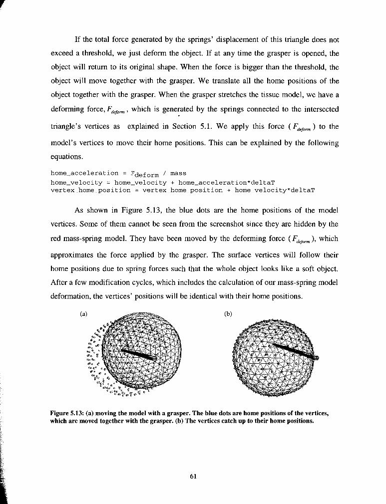
If the total force generated by the springs' displacement of this triangle does not

exceed a threshold, we just deform the object. If at any time the grasper is opened, the

object will return to its original shape. When the force is bigger than the threshold, the

object will move together with the grasper. We translate all the home positions of the

object together with the grasper. When the grasper stretches the tissue model, we have a

deforming force, Fdefo,, which is generated by the springs connected to the intersected

triangle's vertices as explained in Section 5.1. We apply this force ( Fdefo, ) to the

model's vertices to move their home positions. This can be explained by the following

equations.

home-acceleration = Fdeform / mass

home-velocity = home-velocity + home-acceleration*deltaT vertex-home-position = vertex-home-position + home-velocity*deltaT

As shown in Figure 5.13, the blue dots are the home positions of the model

vertices. Some of them cannot be seen from the screenshot since they are hidden by the

red mass-spring model. They have been moved by the deforming force (Fdefo, ), which

approximates the force applied by the grasper. The surface vertices will follow their

home positions due to spring forces such that the whole object looks like a soft object.

After a few modification cycles, which includes the calculation of our mass-spring model

deformation, the vertices' positions will be identical with their home positions.

Figure 5.13: (a) moving the model with a grasper. The blue dots are home positions of the vertices, which are moved together with the grasper. (b) The vertices catch up to their home positions.

5.4 Interaction between cautery hook and model Cautery hooks used in real surgery have a foot pedal as a switch for applying

electrical current. The cautery hook can also be used as a simple hook, which can palpate

a tissue model while the foot pedal is off. 'It can deform the virtual tissue model by the

means we have explained in Section 5.1. Otherwise it can also cut with the hook. We

have implemented a virtual cautery hook model in our simulator. The virtual cautery

hook can be controlled by Immersion Virtual Laparoscopic Interface (VLI), which has a

foot pedal, as shown in Figure 5.14. It can also be controlled by the haptic feedback

device Immersion LapIE. For Immersion LapIE, we implement a virtual foot pedal by

pressing a certain key on keyboard.

Figure 5.14: Immersion Virtual Laparoscopic Interface

For the cutting state, the cut will occur immediately after the hook contacts the

model surface. This is different from the scalpel, which needs to exceed a cutting

threshold in order to cut,. The cautery hook has two cutting edges, AB and BC, as shown

in Figure 5.15. Therefore, collision detection to find the exact cutting intersections

involves checking these two line segments. The L-hook cutting case is more complex

than that for the scalpel, which only has a single cutting edge.

Figure 5.15: Representation of L-hook cautery for collision detection

Figure 5.16 shows sample cutting cases. In (a), both cutting edges intersect with

the tissue model. Here, line segment AB and BC may intersect with the same triangle or

two adjacent triangles or even more triangles. In our current implementation, we take the

lagging edge as the current cutting edge. For instance, suppose AB and BC both intersect

with triangle TI at a given time step, and at the next time step, BC moves out of triangle

T1 and into the neighbour triangle T2, but AB still intersects triangle TI. AB is the

lagging edge in this case. We assume the hook still intersects triangle TI until both AB

and BC have moved out of triangle TI. Figure 5.16(b) is a relatively simple case with

only one cutting edge AB intersecting the model. Figure 5.16(c) is another case where

both AB and BC intersect the model. However, in this case we only use BC as cutting

edge since AB is completely inside the model.

Figure 5.16: Illustrating different cutting states for cautery cutting.

In contrast to the scalpel, a cautery hook can cut in any direction. Therefore, there

is no constraint force in the force feedback model. The force sent back to the user is

composed of a resistant force and a cutting friction force. The method we use to

implement this is similar to that for the scalpel feedback model in Section 5.2.

5.5 Discussion We have implemented haptic feedback models for virtual scalpel, grasper and

cautery L-hook in this thesis work. We also considered several different interactions

between the virtual instrument and the tissue model. With haptic feedback, the user has

more sensation to interact with the virtual reality models.

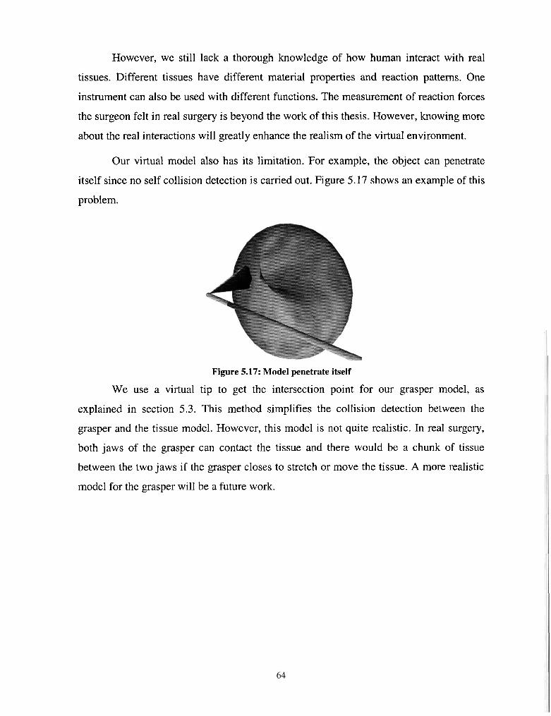
However, we still lack a thorough knowledge of how human interact with real

tissues. Different tissues have different material properties and reaction patterns. One

instrument can also be used with different functions. The measurement of reaction forces

the surgeon felt in real surgery is beyond the work of this thesis. However, knowing more

about the real interactions will greatly enhance the realism of the virtual environment.

Our virtual model also has its limitation. For example, the object can penetrate

itself since no self collision detection is carried out. Figure 5.17 shows an example of this

problem.

Figure 5.17: Model penetrate itself

We use a virtual tip to get the intersection point for our grasper model, as

explained in section 5.3. This method simplifies the collision detection between the

grasper and the tissue model. However, this model is not quite realistic. In real surgery,

both jaws of the grasper can contact the tissue and there would be a chunk of tissue

between the two jaws if the grasper closes to stretch or move the tissue. A more realistic

model for the grasper will be a future work.

Chapter 6

6 A Training Task for Laparoscopic Tissue Dissection

As discussed earlier, virtual environments for training in the skills required for

laparoscopic surgery have been developed in many institutions. However, training in

tissue dissection, a frequently used laparoscopic skill, has not been adequately addressed.

Hence we have developed a virtual module to assist in the training of this elementary

laparoscopic manoeuvre based on the method we developed for tissue dissection

simulation. The module simulates the use of an L-hook laparoscopic cautery tool in tissue

division.

A computer-based training environment has the advantage that trainee

performance can be recorded and forces used in tissue dissection can be analysed. The

lack of standardized performance measures is still a significant problem. We have

therefore defined our own quantitative measures of the skills required for tissue

dissection.

6.1 Task Description The task is to dissect a 3-D tissue model using a simulated L-hook. We integrated

an Immersion LapIE device, which can provide force feedback to the trainee, into our

dissection simulation. The trainee can feel force feedback when the hook contacts virtual

tissue using the haptic device. Our haptic feedback model for the cautery hook was

described in chapter 5. We also integrated a two-handled Immersion Virtual

Laparoscopic Interface (Figure 5.14) into our system. This device lacks haptic feedback,

but has a foot pedal that controls the cautery.

First, a predefined path is drawn on the tissue surface. Second, the trainee, using

one hand stretches the tissue with a grasper and with the other hand dissects along the

path using the L-hook. When the hook contacts the simulated tissue surface while the

foot pedal pressed, the tissue is divided as the L-hook moves through it without

noticeable delay. Figure 6.1 shows a screenshot of one simple dissection task. The line on

the tissue model is the predefined path to be followed.

Figure 6.1: Example of dissection task: (a) Stretch the drawn path before dissection. (b) Make a jagged cut

6.2 Performance Assessment Metrics After consulting a surgeon experienced in laparoscopic surgery, we have defined

three task-based metrics to assess trainee performance:

1) Total deviation of actual cut path from the drawn path.

2) Contact time between the instrument and tissue.

3) Contact discontinuity.

6.2.1 Total deviation of actual cut path from the predefined path Both the predefined path (Figure 6.2(a)) and the path actually cut (Figure 6.2(b))

are represented by a set of straight line segments. The line segments of the cut path are

defined by the intersection points of the instrument and tissue model surface, as shown by

the little spheres in Figure 6.2 (b). To quantify the deviation between two 3D curves, we

project the cut and drawn paths onto XY, YZ and XZ coordinate planes and calculate the

sum of areas between the two sets of projection curves as the deviation.

(a)

The drawn pa

Figure 6.2: Example of the predefined path and the actual cut path

Figure 6.3: Illustration of deviation of actual cut path from the drawn path.

Figure 6.3 shows an example of the deviation of the cut path from the predefined

path when projected to the same coordinate plane. The solid line segments (DID2D3D4)

show the predefined path and the dashed line segments (AIA2A3A4A5) show the cut

path. The area between them, which is the deviation we defined, is illustrated in (a). We

calculate the area by forming triangles between the predefined path with the actual cut

path and calculate the triangles' areas, as shown in Figure 6.3(b). The points of the

predefined path are stored in a list, dPath[], and aPath[] for the actual path points. dPath

and aPath may have different numbers of points and the points may be far away from

each other if the trainee cannot follow the predefined path well. We first try to find the

intersections between the predefined path and the actual path. In this example, as shown

in Figure 6.3 (b), line segment D2D3 intersects with line segment A3A4 at point I. Then

we form triangles between previous points in the two lists, Dl, D2 and Al, A2, A3, using

the same algorithm used to generate groove triangles for a cut (refer to section 4.3.2). The

triangles formed in this way are AlA2D1, D1D2A2 and A2A3D2. For the intersection part,

we calculate the area of the two triangles, D2A31 and A4D31. We repeat this process with

the following points in the lists until we finish the list.

6.2.2 Contact time between instrument and tissue The contact time between instrument and tissue will affect the severity of tissue

burning, i.e. if the cautery hook contacts one place too long, it will be severely burnt. We

define the time that the instrument stays within a certain area while it contacts the tissue

as the contact time. To implement this, we set the first intersection point as reference

point. If the distance from the current intersection point to the reference point is larger

than a threshold, we make the current intersection point the new reference point and take

the elapsed time as the contact time.

6.2.3 Contact discontinuity The novice user may have difficulty in determining the depth while looking at a

2D monitor screen. Therefore, it is possible for them to lift the instrument and lose

contact with the tissue. We consider that as a break in their actual dissection path.

Your performance of this task ........................ YZ deviation from ideal path s : 0.1 11

XZ deviation from ideal path is : 0.115

XV deviation from ided path is : 0.386

Average contact time is : 0.115 ms

Max contact time k : 2.78hs

Total twne IS : 16.533s

Number of contact break in your operation : 0

Number of break you made to the defined path : 1

Figure 6.4: Online performance assessment: (a)Defined path and cut path with assessment dialog. (b)Assessment dialog magnified to make text readable

Assessment results can be shown online and can be saved for further analysis.

Figure 6.4 shows an example of our system's online performance evaluation information.

Figure 0.4(b) shows the performance evaluation message box enlarged for readability.

6.3 Implementation Details In this section we discuss the major technical issues involved in the development

of the training task.

6.3.1 Representation of a path As we mentioned in Section 6.2.1, the path is represented by a set of line

segments, rendered by GL-LINE-STRIP in OpenGL. We treat the predefined path and

the cutting path in the same way. Therefore, in the following section, unless specified

otherwise, path refers to either path. We simplify any path within a triangle by a single

straight line segment connecting the first and the last intersection points in the triangle, as

shown in Figure 6.5. Triangle here refers to the original triangle, before being subdivided

by the cut. We save the intersection points of the instrument and the tissue surface in two

lists, dPath[] for the defined path and aPath[] for the cut path. We allow more than one

path on the tissue surface. However, we use only one list for the defined path and one list

for the cut path. The last intersection point has a flag, "stop", to show it is the end of a

path. Figure 6.5(a) is an example where the path breaks at point 8. Here point 8's stop

flag is set. We start a new line strip from point 9. Figure 6.5(b) is another example of two

paths. Point 9 is the stop point of the first path.

Figure 6.5: Representation of a path by a series of intersection points

6.3.2 Path displacement with tissue stretch We also implemented a grasper model so the user can grasp the tissue and stretch

it. This means we must also deform the path as the tissue surface deforms. The tissue

surface is deformed by moving the vertices to new positions calculated by solving the

mass-spring model. We developed an algorithm using Barycentric coordinates [Math] to

move intersection points along with their containing triangle. Barycentric coordinates

were introduced by F. Moebius in 1827. If we have a set of points, we can define a local

coordinate system to represent a given point and the coordinates systems are Barycentric

coordinates.

We have defined two cases:

Displace cut point with containing edge (since most intersection points lie on

edges, Figure 6.6(a)).

Intersection point is inside a triangle (corresponding to the first and last

intersection points, Figure 6.6 (b)).

Figure 6.6: (a) Displace vertex on edge (b) Displace vertex inside triangle

As shown in Figure 6.6(a), intersection point C is on edge AB. We first calculate

the initial Barycentric coordinate ( a ,P ) for point C as C = a A + P B , where a and P are

scalars and a + P = 1 .Then we can simply displace C together with A and B's new

position. We can calculate a and p as:

length(BC) a= and fl = length( AC)

length(AB) length(AB)

When the intersection point is inside the triangle, e.g. D in triangle ABC (Figure

6.6(b), we represent point D using Barycentric coordinates (u, v, w) as D = uA + vB + wC ,

where u , v and w are scalars and u + v + w = 1 . We calculate u . v and w as:

area(a DCB) area (ADA C) area(a DAB) u = , v = and w =

area(a ABC) area(aABC) area(aABC)

We deform point D along with triangle ABC by calculating its new position using

A, B and C's new position. Figure 6.1 (a) is an example of displacing the predefined path

while the user stretches the model.

6.3.3 Cut along the defined path When the trainee attempts to follow the defined path, helshe may cut through the

defined path. To make the simulator look more realistic, we also developed an algorithm

to divide the defined path as the trainee moves the L-hook through it.

Defined pat\ \ 1

Figure 6.7: Illustration of cutting the predefined path. (a) Defined path and actual cutting path without subdivision. (b) Subdivision applied. (c) Path after subdivision, both the defined path and the cut path have been modified to reflect the cut.

As shown in Figure 6.7(a), the solid line is the predefined path and black dots

represent the intersection points that define the path. The dotted line is the cut path. We

can see the two paths intersect each other, which mean the defined path has been cut. As

explained in chapter 4, the intersected triangles are subdivided to simulate the cut,

resulting in the original triangles being replaced by several small triangles (Figure

6.7(b)). Note that A1 ... A5 are not the actual vertices used to construct the new small

triangles; they are intersection points that record the cut path. For instance, two separate

vertices (L and R) are created at position A2 as subdivision template SE (refer to chapter

4 for detail) applied to triangle ABC. As mentioned in Section 4.3, the intersection points

are either inside a triangle, e.g. D l and Dg, or on edge, e.g. D2, D3 and Dq. When the

triangles are subdivided, all these intersection points need to be modified since the

original triangles and edges no longer exist. We want to keep the number of intersection

points of the predefined path and the actual cutting path almost the same. Therefore,

when the cutting path intersects the defined path ("cuts" it), we do not want to insert a

new point into the defined path list. We use the "stop" flag to reflect the cut made to the

predefined path, i.e. the predefined path becomes two broken paths (see Figure 6.5(a) for

example).

There are two steps to modify the defined path to reflect its being cut. First, we

need to modify the triangle or edge that the point is inside or on. Dl was in triangle ABC

(Figure 6.7) before the cut. It changes to the small triangle after triangle ABC has been

subdivided. D2 changes to the edge connected to vertex B instead of edge BC. This can

be achieved by comparing distance BD2 and BA2. If distance BD2 is smaller than

distance BA2, D2 is on the edge connected to vertex B and A2 keeps the same position as

the left new vertex (L). Otherwise, D2 is on the edge connecting to vertex C. The next

step is to determine whether the intersection point of predefined path is the termination of

one part of the path, i.e. whether its "stop" should be set. For instance, D2 and D3 are on

different sides of line segment A2A3, therefore D2 is a stop. Since D3 and Dq are on the

same side of line segment A3A4, D3 is not a stop. Figure 6.7 (c) shows the result of our

algorithm. Figure 6.2 (b) is a screenshot of an example where the defined path has been

cut.

6.4 Discussion The module we have developed is a novel approach to measuring tissue division

slulls. The module is not a simulation of an actual laparoscopic task but rather a potential

means of developing and assessing the basic skills required for tissue dissection. Whether

following the predefined path helps to acquire laparoscopic surgical skill is still

undetermined.

We set up this training module in Surrey Memorial Hospital, BC and

demonstrated it to a senior surgeon experienced in laparoscopic surgery. The

experimental setup with an Immersion two handled haptic device is shown in Figure 6.8.

The surgeon commented that he felt the design of the task and the three metrics we

defined would be helpful for trainees to gain the basic skills required for tissue dissection.

Laparoscopic surgery is a two-handed process. Since tissue divides better and

easier when it is stretched, the tool in the left hand grasps and stabilises/stretches the

tissue to permit and make easier dissection. Therefore, the surgeon also suggested that

magnitude of the stretching force would be another useful metric in this task. Future work

will include a formal user study to determine effectiveness of the module and

performance metrics as a training method for laparoscopic tissue dissection.

Figure 6.8: Demonstration environment in Surrey Memorial Hospital, BC

Chapter 7

7 Conclusions and Future Directions

7.1 Conclusions In this thesis, we introduce our method of simulating progressive tissue cutting.

Our method can generate virtual arbitrary cuts, which dynamically follow the user-

controlled instrument without noticeable delay. We are the first to detail a progressive

subdivision and re-meshing algorithm based on an enhanced surface mass-spring model

[Zhan03]. The main idea of progressive cutting is to temporarily subdivide the triangle

intersecting the instrument. The subdivision scheme applied to each triangle is

determined by the state of intersection with the instrument. A state machine is introduced

to model the two types of progressive cutting. Our simulator supports two types of

cutting: "cut-into", in which the instrument only penetrates the simulated tissue, and "cut

through" in which the instrument cuts completely through the tissue.

Since standard surface models cannot deal with the interior structure of an object

for creating cutting results, most previous work takes a volumetric approach to simulating

cutting, using for example tetrahedral elements. This thesis also addresses this problem,

introducing a novel algorithm to add interior structure to an object during a cut. We

generate structures in the cutting opening as a function of the depth of instrument

penetration. For cut-into, we use the instrument tip positions at the start and end of the cut

inside one surface triangle to define the bottom of a groove triangle. For cut-through, we

generate side triangles by connecting top and bottom layer intersection points. This

approach opens another direction to simulate cutting, as commented by Alan Liu

[MICC03, MMVR041. The method to subdivide the surface mesh and generate interior

topology is novel and efficient compared to the widely utilized volumetric model.

We also proposed a method to separate the model after cutting and create a new

mesh object for the part cut off, which extends the simulation of cutting to the more

general simulation of dissection. The resulting tissue portions are available for further

dissection and removal. We have not been able to find any detailed description of this in

the literature.

Our dissection environment can support a number of user interface devices that

can manipulate different representations of virtual instruments. Since it is hard to

determine depth while looking at a 2D screen, a sense of touch becomes essential to

surgeons in laparoscopic surgery. Our simulator can also send reaction forces to the user

through a haptic user interface device. We propose a simple force feedback model for

various instruments and interactions, such as scalpel, cautery hook and grasper. The user

can also interact with the system using multiple instruments, currently implemented using

a two-handled device. These techniques can be integrated into training environments for

both open and laparoscopic surgery.

Training in tissue dissection, a frequently used laparoscopic skill, has not been

adequately addressed. Hence we propose a virtual module to assist in the training of this

elemental laparoscopic manoeuvre based on the method we proposed for tissue dissection

simulation. The module simulates the use of the L-hook laparoscopic cautery tool in

tissue division. This module is a novel approach to simulated tissue dissection in that key

components of the module are the measures used to assess tissue division skills, and the

simulation of a tool familiar to laparoscopic surgeons [Zhan04]. A computer-based

training environment has the advantage that trainee performance can be recorded and

forces used in tissue dissection can be analysed. The lack of standardized performance

measures is still a significant problem. We have therefore defined our own quantitative

measures to evaluate the skills required for tissue dissection. Three metrics have been

designed to assess performance. 1) Total deviation of actual cut path from the drawn

path. 2) Contact time between the instrument and tissue. 3) Contact discontinuity.

This thesis as a whole addresses the problem of simulating tissue dissection

operation within a framework of an interactive physically based surgical training

environment.

7.2 Future Directions While we have proposed and implemented a virtual reality surgical training

environment for tissue dissection, there are areas within this research that can be further

explored.

First, the framework of our simulator is still based on a single thread

computational model, which means the visual and haptic rendering must share the CPU

time. As we have mentioned in chapter 2, there exists a mismatch in the update rate

requirements with 30 Hz for the visual display and lOOOHz for high fidelity haptic

feedback. Although we have proposed a method to give more CPU time to the

modification cycle to adjust the different update rate requirements, as described in section

3.1, the haptic rendering process still cannot be guaranteed at lOOOHz update rate.

Therefore, to separate the haptic rendering process from other calculation is a direct step

to solve this problem. This can be achieved by either spreading the calculation to multiple

threads on the same computer or using a separate computer for haptic rendering [MorOl]

[Biel03].

Second, as pointed out by H.W. Nienhuys et al. [NienOl], subdivision methods,

such as those used to simulate progressive cutting, increase the number of triangles in a

mesh, which may increase the calculation load of the relaxation. They may also produce

tiny triangles, which may cause the mass-spring system to become unstable. Tiny

triangles are also problematic for intersection testing. Therefore, it is hard to continue a

cut from the exact position where the previous cut stops. A method to remove tiny

triangles after subdivision is needed.

Third, we have proposed force feedback models for three instruments interacting

with tissue model; a user study to determine whether the haptic feedback is helpful in

training is needed. Also how to make the force feedback similar to the actual forces felt

by the surgeon in real surgery, in the sense of the same magnitude, is still undetermined.

If a user study could validate the effectiveness of adding force feedback to the virtual

training environment, a further step might be a study of the use of haptic feedback to

guide a trainee in correct cutting directions, which might improve the speed of the

training process.

Fourth, the training module we have developed is not a simulation of an actual

laparoscopic operation but rather a means of developing and assessing the basic skills

required for tissue dissection. Whether the predefined path helps a trainee acquire

laparoscopic surgical skill is still to be determined. Future work will include a user study

to determine the effectiveness of the module and performance metrics as a training

method for laparoscopic tissue dissection. In addition, as pointed out by some surgeons,

the force with which they pull and stretch tissue while using the other hand to cut may

greatly affect the dissection result, suggesting using local stress as an additional

performance metric.

Appendix A

Data Structure for Tissue model

In this appendix, we describe the data structure we developed and used in this

thesis work to model tissue. The main advantage of this data structure is that we can

easily access the adjacency information from any primitive, e.g. triangle, vertex or edge.

VRML In order to make it easy for users and experimenters (including the writer) to

define various shapes, we chose the VRML (Virtual Reality Modelling Language) file

format as the means of representing geometric shapes external to our program. VRML is

an open standard for virtual reality on the Internet. One is that one first defines a

geometric shape using any VRML modelling tool (which includes any text editing

program) and then our program reads the VRML text file and converts it into an internal

data structure to make processing more efficient.

Though VRML models have many other properties, such as material and texture,

we only use geometry and topology information, i.e. vertices' coordinates and how they

are connected together. VRML models have an array of points, referred to as vertices in

later descriptions. The "point" is defined by x, y and z coordinates. Then the model uses

an "IndexedFaceSet" to define faces (planar polygons). as a set of indices to points in the

vertex array. The last index of a face is "-I", to distinguish it from the next face.

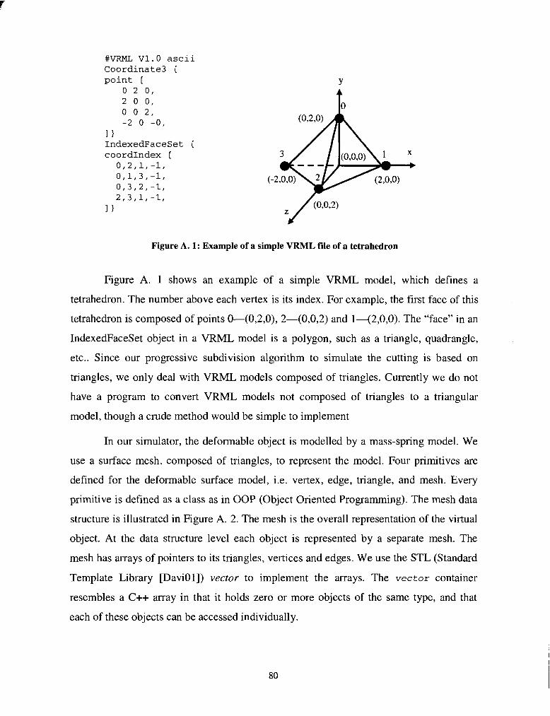
#VRML V1.O ascii Coordinate3 { point [

0 2 0, 2 0 0, 0 0 2, -2 0 -0,

I 1 IndexedFaceSet { coordIndex I

0,2,1,-1, 0,1,3,-1, 0,3,2,-1, 2,3,J-,-18

Figure A. 1: Example of a simple VRML file of a tetrahedron

Figure A. 1 shows an example of a simple VRML model, which defines a

tetrahedron. The number above each vertex is its index. For example, the first face of this

tetrahedron is composed of points 0-(0,2,0), 2-(0,0,2) and 1-(2,0,0). The "face" in an

IndexedFaceSet object in a VRML model is a polygon, such as a triangle, quadrangle,

etc.. Since our progressive subdivision algorithm to simulate the cutting is based on

triangles, we only deal with VRML models composed of triangles. Currently we do not

have a program to convert VRML models not composed of triangles to a triangular

model, though a crude method would be simple to implement

In our simulator, the deformable object is modelled by a mass-spring model. We

use a surface mesh, composed of triangles, to represent the model. Four primitives are

defined for the deformable surface model, i.e. vertex, edge, triangle, and mesh. Every

primitive is defined as a class as in OOP (Object Oriented Programming). The mesh data

structure is illustrated in Figure A. 2. The mesh is the overall representation of the virtual

object. At the data structure level each object is represented by a separate mesh. The

mesh has arrays of pointers to its triangles, vertices and edges. We use the STL (Standard

Template Library [DaviOl]) vector to implement the arrays. The vector container

resembles a C++ array in that it holds zero or more objects of the same type, and that

each of these objects can be accessed individually.

Mesh

Triangle 1

Vertex 1

Figure A. 2: Mesh data structure illustration

Triangle 2

Edge 1

Each triangle has a list of pointers to its vertices and also a list to its edges, as

shown in Figure A. 3

Vertex 2

I Edge 1 I Edge 2 I Edge 3 I .......

Triangle 3

Edge 2

....... I Triangle 1 / Triangle 2 / Triangle 3 / I Triangle N /

Vertex 3

I Vertex 1 I Vertex2 I Vertex3 I ....... 1 Vertex m I

.......

Edge 3

Figure A. 3: Triangle's pointers to its vertices and edges

As shown in Figure A. 4, each vertex has a list of pointers to all the triangles that

Triangle n

.......

surround it. It also has pointers to the edges that connect to it. Therefore, it is easy to find

Vertex m

.......

all the neighbour triangles for a vertex and also all the edges connected to any vertex.

Edge x

Figure A. 4: Vertex's pointers to adjacent triangles and edges

Triangle 1 Triangle 2

Vertex 1

Triangle 3

Vertex 2

....... Triangle N

Vertex 3

Edge 1 .......

.......

Edge x Edge2

Vertex m

Edge 3

Each edge has a pointer to each of the two triangles that share it, and pointers to

its two end vertices, as shown in Figure A. 5.

I Edge 1 I Edge 2 I Edge 3 / . . . . . . .

Triangle 1

1 Vertex 1 I Vertex2 1 Vertex 3 I . . . . . . . I Vertex m I Figure A. 5: Edge's pointers to its end vertices and adjacent triangles

As shown in the illustration, the data structure is complex. However, it saves time

Triangle 2

and effort in accessing the information we need. We describe the primitives (vertex, edge,

and triangle) in detail in the following sections.

Vertex

Triangle N Triangle 3

As shown in Figure A. 6, to represent a 3D vertex, firstly we need its coordinates

(x, y, z). The vertex data object also contains a list of edges that connect to this vertex

and a list of triangles that share this vertex. For the mass-spring model, every vertex is

considered a mass point and all the edges that connect to it act as springs. Therefore,

storing all the pointers to the edges that connect to this vertex within its data structure

enables us to calculate the deformation of the mesh by traversing all the vertices. We will

explain how we calculate the deformation in a later section. The vertex also has a home

position defined as (hx, hy, hz). The home position is the initial set of coordinates of the

vertex when it is created. A vertex's coordinates (x, y, z) may change due to mesh

deformation. We use Phong Shading for graphic rendering. The vertex's normal is the

average of its surrounding triangles' normal. Therefore we store all the triangles that

surround the vertex in its data structure.

.......

Edges

Triangles

Home Position

I normal I

Figure A. 6: Vertex data structure

For example, the vertex 0 in the tetrahedral model (Figure A.

as the following:

x=o; y=2; z=o; vector<edge*> adjacentEdges adjacentEdges [O] = *e01; adjacentEdges [I] = *e02; adjacentEdges [21 = *e03;

vector<triangle*> adjacentTriangles adjacentTriangles [0] = *t021; adjacentTriangles [I] = *t013; adjacentTriangles [2] = *t032; hx=O; hy=2; hz=O;

Edge

Spring Constant

1) can be i llustratec

Figure A. 7: Edge data structure

As shown in Figure A. 7, an edge is defined by two end vertices (Vl, V2). V1 and

V2 are pointers to those two vertices. It also contains two pointers to the two triangles on

each side of this edge. An edge class also has some other properties, such as spring

constant, rest length. To simulate the tension of soft tissue, every mesh spring has

initially been stretched, i.e. its rest length is less than its initial length. Figure A. 8 shows

how the edge class is defined in our system.

class edge {

vertex* vl; vertex* v2; vector<triangle*> adjacentTriangles;

float springK; float restlength; 1

Figure A. 8: Example of how the edge class is defined

Consider edge03 in Figure 1 as an example:

vl = *vertexO; v2 = *vertex3; adjacentTriangles[O] = *triangle032; adjacentTriangles[l] = *triangle013; springK = 2; restLength = 0.7*2.828; //the rest length is set 70% of the edge length

Triangle As shown in Figure A. 9, a triangle is defined by its three vertices (Vl, V2, V3).

V1, V2, and V3 are pointers to those vertices. It also contains a list of pointers to its three

edges. A triangle class also has some other properties, such as normal, current state and

next state. The cutting state defines which subdivision algorithm this triangle will use.

Figure A. 9: Triangle data structure

We use triangle021 in Figure A. 1 as an example:

Triangle

vector<vertex*> vertices

- Vertices

Edges

other propertries

v1 v2 v3

vertices[O]=vertexO; vertices[l]=vertex2; vertices [2 I =vertexl;

vector<edge*> edges edges[Ol=edge02; edges[ll=edge21; edges[2]=edgelO;

Triangles sharing an edge with the current triangle are "edge neighbour" triangles

to the current triangle. The light colour path in Figure A. 10 shows how to find all the

edge neighbour triangles through the data structure.

Figure A. 10: Illustration of finding current triangle's edge neighbor triangle

Figure A. 11 shows our algorithm written in VC++ to find all the edge neighbour

triangles of one triangle. We continue with the tetrahedron in Figure A. 1 as an example:

Edge neighbor triangles of triangle021 are triangle013 (common edge is edgeol),

triangle032 (common edge is edge02), and triangle231 (common edge is edgel2).

//code example to find triangle's edge neighbor vector<triangle*> triangle: :findEdgeNeighbor() {

vector<triangle*> edgeNeighbors; for(int i=O;i<3;i++) {

//if edge's first neighbor triangle is current triangle, then save the other triangle

if(edgesLi1->adjacentTriangles[Ol==this) edgeNeighbors.push~back(edges[il-~adjacent~riangles[l]);

else edgeNeighb~r~.push~back(edges[i]-~adjcent~riangles[O]);

1 return edgeNeighbors;

I

Figure A. 11: VC++ code to find all the edge neighbor triangles of one triangle

If the scalpel moves into the current triangle's edge neighbor triangle, we say the

scalpel goes across that common edge. Figure A. 12 shows the VC++ code to implement

this check.

bool collideEdgeNeighbor(vertex* scalpelTip, vertex* scalpelEnd) {

bool found = false; interV* newV = NULL; vector<edge*>: :iterator eIter=currentTriangle->edges.beginO; while(eIter!=currentTriangle->edges.end() && found==false) {

if( (*eIter)-~adjacentTriangles[0l==currentTriangle) {

newV=Line~IntersectnewV=Line_Intersect_Triangle(scalpelTip,Triangle(scalpelTip,scalpelEnd, (*eIter)->adjacentTriangles[ll);

if(newV!=mL) //if they intersect, save this point {

newv->triangle=(*eIter)->adjacentTriangles[l]; newv->inter-edge=(*eIter); found=true;

1 1 else {

new~=~ine~~ntersect~~riangle(scalpelTip,scalpel~nd, (*e~ter)->adjacentTriangles[O]);

if(newV!=NULL) //if they intersect, save this point {

newv->triangle=(*eIter)->adjacentTriangles[O]; newv->inter-edge=(*eIter); found=true;

1 1

1 return found;

3

Figure A. 12: VC++ code example to check whether the scalpel goes into current triangle's edge neighbor triangle

We also define a simple class for intersection point, interV as used in Figure A.

class interV //intersection point {

float x,y,z; triangle* triangle;//which triangle this point is inside edge* inter-edge;//if this point is on edge, which edge it's on

1

Other triangles, which only share a common vertex with the current triangle, are

called "vertex neighbour" triangles. The light-colour path in Figure A. 13 shows how to

find all the vertex neighbour triangles for vertex V3 of triangle TI .

a list of pointers to the

Figure A. 13: Illustration of finding current triangle's vertex neighbor triangle

Usually the scalpel does not go across a vertex exactly; if the scalpel does go into

a vertex neighbour triangle we deem the scalpel to cross the vertex shared by these two

triangles. The instruments move slowly at the surgical site. Hence, movements of the

instruments are assumed to be continuous and smooth so collision detection can be

continued locally with neighbouring triangles of the currently intersected triangle. How

the scalpel goes in or out of a triangle, i.e. by an edge or vertex, will change the

subdivision state applied to the triangle. For example, in the tetrahedral model (Figure A.

l), vertex neighbour for triangle021 via vertex0 are triangle013 and triangle032.

Mesh We generate vertices and triangles of the mesh when we read a VRML file. When

we subdivide a triangle to simulate the cut, we actually generate new vertices and

triangles to replace the subdivided triangle. However, when we create these vertices and

triangles, they do not have adjacency information and edges have not been created yet.

Therefore, we need a program to generate edges and the adjacency information. The

following code shows how we implement this.

//generate the mesh geometry relationship, adjacent triangles of vertex, //edges. Initialize the natural length and how much it is stretched of //every edge. This function is called after every cut to update the //mesh topology . . . . . . . . . . . . . . . . . . . . . . . . . . . . . . . . . . . . . . . . . . . . . . . . . . . . . . . . . . . . . . . . . . . . . . . mesh::buildMesh(double meshSpringK, double rest)

/ / The following variables are used to store the two vertices / / in an edge vertex* oldVert; vertex* curvert; edge* curEdge;

for(triIter= triangles.begin0; triIter!=triangles.end(); triIter++) {

vector<vertex*>::iterator vertIter = (*triIter)->vertices.begin();

oldvert = *vertIter; curVert = *vertIter; //----------------in each triangle . . . . . .................... for(; vertIter!=(*triIter)->vertices.end(); vertIter++) {

oldVert = curVert; curVert = *vertIter;

/ / Put this triangle into the triangle vector of / / this vertex (*ver t I ter)-~adjacentTriangles .push_back(*tr i I ter) ;

/ / If the current vertex is not the first one in / / this triangle, we need to build an edge and update / / the edge. if(distance((*triIter)->vertices.begin(), vertIter) > 0) {

boo1 edgeExist = false;

/ / Check if it is needed to create a new edge. / / If this edge exists, curVert should be a vertex / / of the edges in oldVertls adjacentEdges. for(edge1ter = oldvert->adjacentEdges.begin();

edgeIter!= oldvert-radjacentEdges.end(); edgeIter++)

{ if( (*edgeIter)->vl==curVert I I

(*edgeIter)->v2==curVert ) {

edgeExist = true; curEdge = *edgeIter;

I I

/ / We only need to check duplication for one of the two / / vertices. If this edge exists in adjacentEdges in / / either of its vertices, we discard the newly created / / one and use the old one. if (!edgeExist) {

/ / Create and put new edge into orgMesh curEdge = new edge(oldVert, curvert); edges.push-back(curEdge); oldVert-~adjacentEdges.pusholdvert->adjacentEdges.push_back(curEdgeba~k(~urEdge);

/ / Put this edge into edge vector of the current / / triangle

(*triIter)-~edges.pusho->eages.push_back(curEdge);ba~k(~urEdge);

/ / Put the current triangle into the triangle vector / / of this edge curEdge-~adjacentTriangles.pushcurEdge->adjacentTriangles.push_back("trba~k(*triIter~;

/ / Put the two vertices to edge vl,v2, this is / / already done when this edge is created. 1

1

/ / Build the edge consisting of the last vertex and the / / first vertex in this triangle / / Note that at this moment curVert is the last vertex. oldvert = curVert; curvert = *((*triIter)->vertices.begin() ) ;

/ / There is no need to put the current triangle into the / / triangle vector of curVert, because this has been done. / / Check if it is needed to create a new edge. / / If this edge exists, curVert should be a vertex of the / / edges in oldVertts adjacentEdges. boo1 edgeExist=false; for(edge1ter = oldvert->adjacentEdges.begin();

edgeIter!= oldvert->adjacentEdges.end(); edgeIter++)

if( (*edgeIter)->vl==curVert I I (*edgeIter)->v2==curVert )

{ edgeExist = true; curEdge = *edgeIter;

1 1

/ / Put new edges into orgMesh if(!edgeExist) {

curEdge = new edge(oldVert, curvert); edges-push-back(curEdge1; oldvert->adjacent~dges.push_back(curEdge); curvert->adjacentEdges.push_back(curEdge);

1

/ / Put this edge into edge vector of the current triangle (*triIter)-~edges.push~back~curEdge);

/ / Put the two vertices to edge vl,v2, this is already done / / when this edge is created.

/ / Put the current triangle into the triangle vector of / / this edge curEdge-~adjacentTriangles.pushcurEdge->adjacentTriangles.push_back(*trba~k(*triIter);

for (vector<edge*>::iterator e=edges.begin(); e!=edges.end();e++) {

float length= ( *e) ->getlength ( ) ; //how much the spring is stretched (*e)->natualLength=rest*length; (*e) ->springK=meshSpringK/(*e)->natualLength;

Appendix B

Line-Segment and Triangle intersectioni

As we mentioned in section 3.4, we use a simplified representation for our virtual

instrument in collision detection. For collision detection, the virtual instruments are

represented by a small set of line segments. Our virtual tissue model is composed of

triangles, which represent the outer surface of the tissue. Therefore, collision detection

between instrument and tissue model is done by line segment and triangle intersection

checking. In this appendix, we explain the algorithm to find the intersection point.

The simple case of finding the intersection point between a line segment and a

triangle is to find the intersection between the line, on which the given line segment lies,

and the plane that contains the triangle. To do this, we first check whether the line and

plane are parallel. If they are not parallel, there must be an intersection point. Then we

need to check whether this intersection point lies along the line segment and lies within

the triangle.

- -- -

1 This algorithm is a well established mathematical algorithm. The description of this algorithm is referenced to "Determining whether a line segment intersects a 3 vertex facet", written by Paul Bourke, available at h t t ~ : / / a s t r o n o m y . s w i n . e d u . a u / - ~ b o u r k e / ~ , visited at March 2,2004.

We represent the line by equation p = p, + t ( p , - p , ) , where p, and p, are two

known points on the line. The plane is represented by equation Ax + By + Cz + D = 0 ,

where the values of A, B, C are the components of the plane normal, which can be found

by taking the cross product of any two normalized edge vectors. However, for graphic

rendering purpose, we have already calculated normals for every triangle. Therefore, we

can easily get the values of A, B, C for every triangle. D can be found by substituting one

vertex into the equation for the plane as the following:

To find the intersection point p , we just need to find the value for t .

If the denominator above A(<, - P,,) + B ( 4 , - 4, ) + C ( 4 , - 4,) is zero, then the

line is parallel to the plane and they do not intersect. For the intersection point to lie on

the line segment t must be between 0 and 1.

Then we need to check whether this intersection point is inside the triangle. If a

point is inside a triangle, the sum of the internal angles is 277, while a point outside the

triangle has lower angle sums.

As illustrated in the above figure, we want to test whether point P is inside

triangle PaPbPc. We can calculate the angles as the following:

a1 = acos(P,, Po,) Po1 =(%-P)lI(P,-P)I a 2 = acos(e, Po3) where P,, = ( P , - P) 1 I (4 - p) I a3 = acos(P,, Pol) Po3 =(pC-P)lI(pC-P)I

If the sum of a l , a2 and a3 is equal to 2n, point P is inside the triangle. In

computer, we need consider the floating error. Therefore, we approximate this as the

following:

sum = a l+a2+a3; i f (abs(sum-2*3.14)< eps )

r e t u r n t r u e ;

where eps is floating error we can accept.

Appendix C

Axis Aligned Bounding Box (AABB)

To speed up the collision detection, we use Axis Aligned Bounding Box (AABB)

to narrow down our search scope before we find the actual intersection point. AABB is

bounding box whose sides are parallel to the coordinate axes, as shown in the following

figure. We form bounding box around the probe tip. We check with every vertex of the

mesh to see whether it falls inside the bounding box. If a vertex is inside the bounding

box, we save it to the candidate contact vertex list for further checking. Once we find all

the candidate contact vertices, we use line triangle intersection method to check whether

the probe has actually intersected with a triangle that is adjacent to the candidate vertex.

In this way, we can find the exact intersection of the probe and the tissue mesh.

The radius (edge) of the bounding box is twice the length of the longest edge of

the mesh. It can be illustrated by the following pseudo code:

boundingBoxMin[3], boundingBoxMax[3]; //set longest edge's length as the collision detection radius for (i=O; i<3; i++) I

boundingBoxMin[i] = probeTipPosition[i]- LongestEdgeLength; boundingBoxMax[il = probeTipPosition[il+ LongestEdgeLength;

1

for( each node of the mesh) //bounding box checking algorithm {

currentposition = node->GetcurrentPosition(); if ((currentP0sition.x >= tipBoxMinVertex.x) &&

(currentP0siti0n.x <= tipBoxMaxVertex.x) && (currentPositi0n.y >= tipBoxMinVertex.y) && (currentPositi0n.y <= tipBoxMaxVertex.y) && (currentPosition.z >= tipBoxMinVertex.z) && (currentPosition.z <= tipBoxMaxVertex-z))

Save this node into candidateContactList; 1

for( each node in the candidateContactNodeList)

for( each adjacent triangle of aNodeInCandidateList) {

~ine~riangle~ntersectTest(probe,aAdjacentTriangle) if( a contact node is detected) {

set the current contact node/face; return true;

1 1

1

Since our tissue model is deformable, every time step the vertices' position may

change. Contrary to the traditional way to form bounding boxes around every mesh

vertex, we form bounding box around the probe tip. Therefore, every sampling time, we

only need to recalculate the bounding box using current probe tip position. An AABB-

based algorithm is fast since only six comparisons are needed. The time for AABB

checking is linear to the number of mesh vertices. However, if the probe moves too fast,

i.e. during one sampling time, it passes a distance more than the bounding box edge and

may miss the candidate vertex. Since our program runs at a quite high update rate, e.g.

more than IOOHz, this case will not actually happen.

Bibliography

1. [Ahlb02] Ahlberg G., Heikkinen T., Iselius L., Leijonmarck C.E., Rutqvist J., Arvidsson D.,

"Does Training in a Virtual Reality Simulator Improve Surgical Performance?". In Surg

Endosc (2002) 16: 126-129,2002.

2. [Ast198] Astley Oliver R., Hayward Vincent, "Multirate Haptic Simulation Achieved by

Coupling Finite Element Meshes through Norton Equivalents". In Proc. Of IEEE International

Conf. on Robotics and Automation, 1998, pp 989-994.

3. [Auli99] dlAulignac, D., C. Laugier and M. C. Cavusoglu, "Towards a realistic echographic

simulator with force feedback", Proceedings of the 1999 IEEEJRSJ International Conference

on Intelligent Robots and Systems, pp. 727-732.

4. [AuliOO] d7Aulignac, D., R. Balaniuk and C. Laugier, "A Haptic Interface for a Virtual Exam

of the Human Thigh", Proceedings of the 2000 IEEE International Conference on Robotics &

Automation, San Francisco, April 2000, pp. 2452-2457.

5. [Avi196] Avila R.S. and Sobierajski L. M. "A haptic interaction method for volume

visualization". Proceedings of VisualizationP6, pages 197-- 204, 1996.

6. [Barb021 Barbagli F., Prattichizzo D., Salisbury K., "Multirate Analysis of Haptic Interaction

Stability with Deoformable Objects". In Proc. Of IEEE Conf. on Decision and Control, 2002,

Las Vegas, USA, pp 917-922.

7. [Basd99] Basdogan, C., Ho, C., and Srinivasan, M.A. "Simulation of Tissue Cutting and

Bleeding for Laparoscopic Surgery Using Auxiliary Surfaces". Medicine Meets Virtual

Reality (MMVR 99). IOS Press, Amsterdam 1999,38-44.

8. [BasdOl-1] Basdogan C. and Srinivasan M. A., "Haptic rendering in virtual environments," in

Virtual Environments HandBook, K. Stanney, Ed., 2001, [Online]. Available:

9. [BasdOl-21 Basdogan C., Ho Chih-Hao, and Srinivasan M.A., "Virtual Environments for

Medical Training: Graphical and Haptic Simulation of Laparoscopic Common Bile Duct

Exploration". IEEWASME Transactions on Mechatronics, Vol. 6, No. 3, Sept 2001, pp 269-

285.

10. [Bie199] Bielser D., V. A. Maiwald, and M. H. Gross, "Interactive cuts through 3dimensional

soft tissue", in Computer Graphics Forum (Eurographics '99), the Eurographics Association

and Blackwell Publishers, 1999. vol. 18(3), 3 1-38.

11. [BielOO] Bielser, D., M. H. Gross, "Interactive Simulation of Surgical Cuts", Proceedings of

Pacific Graphics 2000. IEEE Computer Society Press, 116-125.

12. [Biel02] Bielser, D., M. H. Gross. Open Surgery Simulation. Proceedings of Medicine Meets

Virtual Reality 2002, IOS Press.

13. [BroN99] Bro-Nielsen M., Tasto J.L., Cunningham R., Merril G.L. "PreOp Endoscopic

Simulator: a PC-based imrnersive training system for bronchoscopy." MMVR 7, 1999.

14. [BrowOl]Brown, J; Sorkin, S; Bruyns, C; Latombe, JC, Montgomery, K; Stephanides, M;

"Real-Time Simulation of Deformable Objects: Tools and Application", Computer Animation

2001, Seoul, Korea, November 7-8,2001.

15. [BruyOl-11 Bruyns C, Senger S., "Interactive cutting of 3D surface meshes", Computer and

Graphics 2001; 25:635-642.

16. [BruyOl-21 Bruyns C, Senger S., Wildermuth S., Montgomery K, Boyle R, "Real-time

interactions using virtual tools", in Proceedings of MICCAI 2001, Niessen WJ et al.(eds).

Springer: Berlin, 2001; 1349-135 1.

17. [Bruy02] Bruyns, C; Montgomery, K; "Generalized Interactions Using Virtual Tools Within

the Spring Framework: Cutting" Medicine Meets Virtual Reality (MMVR02), Newport Beach,

CA, January 23-26,2001.

18.[Boux00]Boux Francois de Casson and Laugier Christian, "Simulating 2D Tearing

Phenomena for Interactive Medical Surgery Simulators", in Proc. of Computer Animation'

2000 May 3-5,2000. University of Pennsylvania, Philadelphia, PA USA.

19. [Cao991 Cao C.G.L., MacKenzie C.L., Ibbotson J.A., Turner L.J., Blair N.P., and Nagy A.G..

"Hierarchical decomposition of laparoscopic procedures". In Proceedings of MedicineMeets

Virtual Reality (MMVR), pages 83-89. IOS Press, 1999.

20. [CavuOO] Cavusoglu M.C., and Tendick Frank, "Multirate Simulation for High Fidelity Haptic

Interaction with Deformable Objects in Virtual Environments". In Proc. Of IEEE International

Conf. on Robotics and Automation 2000, Vol. 3, pp 2458-2465.

21. [CotiOO] Cotin S., Delingette H., and Ayache N., "A Hybrid Elastic Model allowing Real-

Time Cutting, Deformations and Force-Feedback for Surgery Training and Simulation". In

The Visual Computer, 2000, 16(8): 437-452.

22. [Coti02] Cotin S, Stylopoulos N, Ottensmeyer M, Neumann P, Rattner D, Dawson S. "Metrics

for Laparoscopic Skills Trainers: The Weakest Link!". In: Dohi T and Kikinis R, eds.

Proceedings of MICCAI 2002, Lecture Notes in Computer Science 2488, 35-43, Springer-

Verlag, Berlin. 2002.

23. [DaviOl] David R. Musser, Gillmer J. Derge, Atul Saini, "The STL tutorial and reference

guide: C++ programming with the standard template library". Boston, MA: Addison-Wesley,

200 1.

24. [Daws02] Dawson S.L., "A Critical Approach to Medical Simulation". In Bulletin of the

American College of Surgeons, Vol.87, Number 11,2002.

25. [FaraOO] Ali Faraz, Shahram Payandeh, "Engineering approaches to mechanical and robotic

design for minimally invasive surgery (MIS)". Boston : Kluwer Academic, c2000.

26. [Gall011 Gallagher A.G., Richie K., McClure N., and McGuigan J. "Objective psychomotor

skills assessment of experienced, junior, and novice laparoscopists with virtual reality". World

Journal of Surgery, 25: 1478-1483,2001.

27. [Gal1021 Gallagher AG, Satava RM. "Virtual reality as a metric for the assessment of

laparoscopic psychomotor skills. Learning curves and reliability measures". Surg Endosc.

2002, Dec. 16 (12): 1746-52. Epub 2002 Jul29.

28. [GanoOO] Ganovelli F., P.Cignoni, C.Montani and R.Scopigno, "Enabling Cuts on

Multiresolution Representation". Proceedings of CGI (Computer Graphics International)

2000, 183-191.

29. [Gorm99] Gorman Paul J., Meier Andreas H., Krurnmel Thomas M., "Simulation and Virtual

Reality in Surgical Education - Real or Unreal?" In ARCH SURGNol 134, Nov 1999,

pp.1203-1208. Available at www.archsurg.com.

30. [HaluOl] Haluck R., Webster R., Snyder A., Melkonian M., Mohler B., Dise M., LeFever

A., "A Virtual Reality Surgical Trainer for Navigation in Laparoscopic Surgery", Proceedings

of the Medicine Meets Virtual Reality Conference, (MMVR '2001), Newport Beach,

California, IOS Press, January 24-27,2001, pp. 171-176.

31. [Hiro99] Hirota Koichi, Tanaka Atsuko, Kaneko Toyohisa, "Representation of Force in

Cutting Operation", IEEE Virtual Reality, March 13 - 17, 1999, Houston, Texas, page 77.

32. [Irnme] Immersion Corporate, Product Literature. URL: www.irnrnersion.com.

33. [John] Johnston R., Bhoyrul S., Way L., Satava R., McGovern K., Fletcher J. D., Range1 S.,

and Loftin R. B., "Assessing a Virtual Reality Surgical Skills Simulator". Available at

httv://www.vmasc.odu.edu/vetVhtmVsur~, visited Jan loth, 2004.

34. [JordOl] Jordan J.A., Gallagher A.G., McGuigan J., and McClure N., "Virtual reality training

leads to faster adaptation to the novel psychomotor restrictions encountered by laparoscopic

surgeons". Surgical Endoscopy, 15: 1080-1084,2001.

35. [KuhnOO] Kuhnapfel U., Cakrnac H.K., MaaP H., "Endoscopic Surgery training using virtual

reality and deformable tissue simulation", Computers & Graphics, 2000, Vol. 24, pp. 671-682.

36. [Lapa] Laparoscopy Hospital, Available at httv://www.lavaroscov~hosvital.com~add.htm,

visited on Nov. 17,2003

37. [Liu03] Liu Alan, Tendick Frank, Cleary Kevin, Kaufmann Christoph, "A Survey of Surgical

Simulation: Applications, Technology, and Education". In Presence, Vol 12, Issue 6,

published by the MIT Press.

38. [MahvOl] Mahvash, M., Hayward, Haptic Rendering of Cutting: a Fracture Mechanics.

Haptics-e, http://www.haptics-e.org/. Vol. 2, No. 3. V. 2001.

39. [Mark961 W. R. Mark, S. C. Randolph, Mark Finch, J. M. V. Verth, R. M. Taylor, "Adding

Force Feedback to Graphics Systems: Issues and Solutions". In SIGGRAPH'96 Proceedings,

pp 447-452.

40. [Mass941 Massie T.H., Salisbury J.K., "the PHANTOM Haptic Interface: a Device for Probing

Virtual Objects", ASME Winter Annual Meeting, Symposium on Haptic Interfaces for Virtual

Environments and Teleoperator Systems. November 1994. Chicago, Illinois, pp295-299.

41. [Math] Barycentric coordinates. Available at:

http://mathworld.wolfram.com~BarycentricCoordinates.html, visited on Mar. 6", 2004.

42. [Ment] Mentice Corporation, URL: www.mentice.com.

43. [Mese97] Meseure P., Chaillou C. "Deformable Body simulation with Adaptive Subdivision

and Cuttings". Proceedings of the WSCG'97, Plzen, 10-14 February 1997, pp 361-370.

44. [Metho21 Mehta, N., Haluck, R., Frecker, M., and Snyder, A., "Sequence and Task Analysis

of Instrument Use in Common Laparoscopic Procedures," Surgical Endoscopy Ultrasound and

Interventional Techniques, 2002, 16: 280-285.

45. [MICC03] Alan Liu, Stephane Cotin, M. Cenk Cavusoglu, Mark Bowyer, MICCAI 2003

Tutorial: Simulation for Medical Education. Available at http://www.simcen.org;/miccai2003/,

visited Feb. 25th, 2004.

46. [MMVR04] Alan Liu, M. Cenk Cavusoglu, Stephane Cotin, Mark Bowyer, MMVR 2004

Tutorial: Medical Simulation Tutorial: The State-of-the-Art and Beyond. Available at

http://www.simcen.orp/mmvr2004/, visited Feb.25th, 2004.

47. [Mont02]Montgomery, K; Bruyns, C; Brown, J; Thonier, G; Tellier, A; Latombe, JC; "Spring:

A General Framework for Collaborative, Real-Time Surgical Simulation", Medicine Meets

Virtual Reality (MMVR02), Newport Beach, CA, January 23-26,2001.

48. [Mood03] Moody, L. Baber, C. Arvanitis, T.N. Elliott, M. "Objective Metrics for the

Evaluation of Simple Surgical Skill in Real and Virtual Domains". Presence: Teleoperators

and Virtual Environments 12 (2), April 2003.

49. [MorOl] Mor, A., Kanade, T. "Modifying Soft Tissue Models: Progressive Cutting With

Minimal New Element Creation". MICCAI 2000, LNCS 1935,598-607.

50. [Morg96] Morgenbesser, H. B. and M. A. Srinivasan (1996). Force shading for haptic shape

perception. ASME Dynamic Systems and Control Division, (DSC-Vol.58): 407-412.

51. [NienOl] Nienhuys Han-Wen and A. Frank van der Stappen. "Supporting cuts and finite

element deformation in interactive surgery simulation". In Proceedings of MICCAI'Ol,

Niessen WJ et al.(eds). Springer: Berlin, 2001; 145-152.

52. [Ota] Ota D., Loftin B., Saito T.,Lea R., Keller J., "Virtual Reality in Surgical Education".

Available at http:Nwww.vmasc.odu.edu/vetYht~ur~ery/vrse.html, visited Jan loth, 2004.

53. [Patr92] Patrick J. "Training: Research and Practice". London: Academic Press. 1992.

54. [Paya02] Payandeh S., Lomax A. J., Dill J., Mackenzie C.L., "On defining metrics for

assessing laparoscopic surgical skills in a virtual training environment", Proceedings of

MMVR 2002, IOS press 2002.

55. [Paya03] Payandeh S., Dill J., Wilson G., Zhang H., Shi L., Lornax A., MacKenzie C.. "LTE:

A Multi-Modal Training Environment for Surgeons." Proceedings of the Fifth International

Conference on Multimodal Interfaces. November 2003.

56. [PiciOO] Picinbono G., Delingette H., and Ayache N., "Improving Realism of a Surgery

Simulator: Linear Anisotropic Elasticity, Complex Interactions and Force Extrapolation".

Technical report RR-4018, INRLA, 2000

57. [Rein961 Reinig Karl D., Rush Charles G., Pelster Helen L., Spitzer Victor M., Heath James

A., "Real-Time Visually and Haptically Accurate Surgical Simulation". Healthcare in the

Information Age. 1996,542-546.

58. [Rose021 Rosen J., Solazzo M., Hannaford B., Sinanan M., "Objective Evaluation of

Laparoscopic Skills Based on Haptic Information and Tool/Tissue Interactions", Computer

Aided Surgery, Vol. 7 (I), pp. 49-61 July 2002.

59. [Rose031 Rosen J., Chang L., Brown J.D., Hannaford B., Sinanan M., Satava R., "Minimally

Invasive Surgery Task Decomposition- Etymology of Endoscopic Suturing". In Proceedings

of MMVR 2003, IOS press 2003.

60. [Rusp97] Ruspini D., Kolarov K., and Khatib O., "The haptic display of complex graphical

environments". SIGGRAPH Proceedings, 1997, 345-352.

61. [Sali95] Salisbury K., Brock D., Massie T., Swamp N., and Zilles C., "Haptic Rendering:

Programming Touch Interaction with Virtual Objects". In Proc. Of ACM 1995 Symp. On

Interactive 3D Graphics, pp 123-130.

62. [Seym02] Seymour NE, Gallagher AG, Roman SA, O'Brien MK, Bansal VK, Andersen DK,

Satava RM, "Virtual reality training improves operating room performance: results of a

randomized, double-blinded study". Ann Surg. 2002 Oct; 236(4):458-63; discussion 463-4.

63. [SmitOO] Smith S., Torkington J., Taffinder N. and Darzi A., "The objective assessment of

surgical skill", Min. Invas. Ther. & Allied Tech., 2000: 9(5) 315-320.

64. [Srin97] Srinivasan M.A., Basdogan C., "Haptics in virtual environments: Taxonomy,

research status, and challenges". Computers and Graphics, 1997, Vol. 21,393-404.

65. [STL] "The STL tutorial and reference guide: C++ programming with the standard template

library" / David R. Musser, Gillmer J. Derge, Atul Saini. Boston, MA: Addison-Wesley, 2001.

66. [Sty1031 Stylopoulos N., Cotin S., Dawson S., Ottensmeyer M., Neumann P., Bardsley R.,

Russell M., Jackson P., Rattner D., "CELTS: A clinically-based Computer Enhanced

Laparoscopic Training System". In Proceedings of MMVR 2003.

67. [Surg] Surgical-Science. www.surgica1-science.com

68. [Tana98] Tanaka, A., Hirota, K., Kaneko, T., "Virtual Cutting with Force Feedback", Virtual

Reality Annual International Symposium, 1998, Proceedings IEEE 1998,71 -75.

69. [TendOO] Tendick F., Downes M., Goktekin T., Cavusoglu M.C., Feygin D., Wu Xunlei, Eyal

R., Hegarty M., Way L.W., "A Virtual Environment Testbed for Training Laparoscopic

Surgical Skills". In Presence, Vol. 9, Issue 3, June 2000, pp.236-255.

70. [Voss99] Voss, G., Hahn, J.K., Muller, W., Lineman, R.W. "Virtual Cutting of Anatomical

Structures". Medicine Meets Virtual Reality, IOS Press, Amsterdam, 1999.

71. [Wong98] Wong Kevin CH, Siu Tommy YH, Heng PA, Sun Hanqiu, "Interactive Volume

Cutting", in Proc. of Graphic Interface'98, Vancouver, British Columbia, June 1998, pp. 99-

105.

72. [Zhan02-11 Zhang, J., S. Payandeh and J. Dill, "Haptic subdivision: an Approach to Defining

Levels of Details in Haptic Rendering", Proceedings of the 1 0 ~ Symposium on Haptic

Interfaces for Virtual Environment and Teleoperator Systems, Orlando, FL, March, 2002,

pp20 1-208.

73. [Zhan02-21 Jian Zhang, "Efficient haptic rendering of deformable objects and haptic aided

design ". M.A.Sc. Thesis, Simon Fraser University, 2002.

74.[Zhan03] Hui Zhang, Payandeh Shahram, and Dill John. "The look and feel of virtual

progressive cutting." Proceedings of the 9th International Conference on Virtual Systems and

Multimedia, October 2003, p.764-p.771.

75. [Zhan04] Hui Zhang, Shahram Payandeh, John Dill, Alan J.Lomax. "Acquiring laparoscopic

manipulative skills: A virtual tissue dissection training module". To be presented in The 12th

Annual Medicine Meets Virtual Reality Conference, January 2004.

76. [Zi1194] Zilles C.B., Salisbury J.K., "A Constraint-based God-object Method for Haptic

Display". ASME Haptic Interfaces for Virtual Environment and Teleoperator Systems 1994,

Dynamic Systems and Control 1994 (Chicago Illinois, Nov.6-l l), vol. 1, pp146-150.