simulating rainfall time-series: how to account for
TRANSCRIPT
ORIGINAL PAPER
Simulating rainfall time-series: how to account for statisticalvariability at multiple scales?
Fabio Oriani1 • Raj Mehrotra2• Gregoire Mariethoz3
• Julien Straubhaar4•
Ashish Sharma2• Philippe Renard4
Published online: 11 April 2017
� Springer-Verlag Berlin Heidelberg 2017
Abstract Daily rainfall is a complex signal exhibiting
alternation of dry and wet states, seasonal fluctuations and
an irregular behavior at multiple scales that cannot be
preserved by stationary stochastic simulation models. In
this paper, we try to investigate some of the strategies
devoted to preserve these features by comparing two recent
algorithms for stochastic rainfall simulation: the first one is
the modified Markov model, belonging to the family of
Markov-chain based techniques, which introduces non-
stationarity in the chain parameters to preserve the long-
term behavior of rainfall. The second technique is direct
sampling, based on multiple-point statistics, which aims at
simulating a complex statistical structure by reproducing
the same data patterns found in a training data set. The two
techniques are compared by first simulating a synthetic
daily rainfall time-series showing a highly irregular alter-
nation of two regimes and then a real rainfall data set. This
comparison allows analyzing the efficiency of different
elements characterizing the two techniques, such as the
application of a variable time dependence, the adaptive
kernel smoothing or the use of low-frequency rainfall
covariates. The results suggest, under different data
availability scenarios, which of these elements are more
appropriate to represent the rainfall amount probability
distribution at different scales, the annual seasonality, the
dry-wet temporal pattern, and the persistence of the rainfall
events.
Keywords Rainfall � Simulation � Markov chain � Multiple
point statistics � Long-term � Time-series
1 Introduction
It has been observed that daily rainfall can have a chaotic
behavior (Basu and Andharia 1992; Jayawardena and Lai
1994; Sivakumar et al. 1998, 2001; Millan et al. 2011;
Jothiprakash and Fathima 2013; Sivakumar et al. 2014),
requiring high-order statistical or deterministic models
(Schertzer et al. 2002; Khan et al. 2005) to generate real-
istic simulations and reliable short- and long-term
predictions.
The Markov-chain (MC) family of techniques is one of
the most common stochastic approach to simulate daily
rainfall since the 60’s (Gabriel and Neumann 1962),
treating rainfall occurrence and amount separately as two
joint random variables. The simulation of both quantities is
usually sequential and conditional to recent past (low-order
time dependence). The drawback of classical daily Markov
models is the under-representation of the variance of
monthly and annual historical wet days and rainfall totals
(Buishand 1978; Wilks 1989), an issue known as overdis-
persion. Even the use of higher-order dependence under-
estimates higher time-scale variances (Katz and Parlange
1998), while dramatically increasing the number of
parameters. A key improvement has been brought to the
latest generation of MC based algorithms, introducing non-
& Fabio Oriani
1 Department of Hydrology, Geological Survey of Denmark
and Greenland, Øster Voldgade 10, 1350 Copenhagen K,
Denmark
2 School of Civil and Environmental Engineering, University
of New South Wales, Sydney, Australia
3 Institute of Earth Surface Dynamics, Universite de Lausanne,
Lausanne, Switzerland
4 Centre for Hydrogeology and Geothermics, Universite de
Neuchatel, Neuchatel, Switzerland
123
Stoch Environ Res Risk Assess (2018) 32:321–340
https://doi.org/10.1007/s00477-017-1414-z

stationary parameters consistent with the underlying recent
past variations. In particular, the daily rainfall occurrence
probability is conditioned using either exogenous climatic
variables, for example large-scale atmospheric indicators
(Hay et al. 1991; Bardossy and Plate 1992; Katz and Par-
lange 1993; Woolhiser et al. 1993; Hughes and Guttorp
1994; Wallis and Griffiths 1997; Wilby 1998; Kiely et al.
1998; Hughes et al. 1999; Buishand and Brandsma 2001),
lower-frequency daily rainfall covariates (Wilks 1989;
Briggs and Wilks 1996; Jones and Thornton 1997; Katz
and Zheng 1999) or indexes based on the recent past
rainfall behavior (Harrold et al. 2003a, b; Mehrotra and
Sharma 2007a, b) to simulate the low-frequency fluctua-
tions observed in the training data set. An alternative
strategy allowing the preservation of the mean and variance
at multiple scales is model nesting (Wang and Nathan
2002; Srikanthan 2004, 2005; Srikanthan and Pegram
2009), which involves the correction of the generated daily
rainfall using a multiplicative factor to compensate the
low-order moments bias at the monthly and annual scales.
In this paper, we compare two of the few techniques
proposed in the literature that can preserve rainfall statistics
up to the decennial scale without any additional informa-
tion apart from the historical daily rainfall time-series. The
first one, representative of the latest generation of MC
based algorithms, is the modified Markov model (Mehrotra
and Sharma 2007a; Mehrotra et al. 2015), which conditions
the Markov chain parameters on the number of past wet
days to impart the low frequency fluctuations. The second
one is direct sampling (Mariethoz et al. 2010), belonging to
multiple-point statistics (MPS), a family of geostatistical
techniques widely used in spatial data simulation (Guar-
diano and Srivastava 1993; Strebelle 2002; Zhang et al.
2006; Arpat and Caers 2007; Honarkhah and Caers 2010;
Straubhaar et al. 2011; Tahmasebi et al. 2012; Straubhaar
et al. 2016). MPS algorithms are based on the concept of
training data set (or training image, TI): a data set repre-
sentative of the simulated variable used to infer the
occurrence probability of each event conditionally on
multiple neighbor points. This high-order conditioning
allows respecting a complex covariance structure by
reproducing the same type of patterns as found in the TI at
multiple scales. The direct sampling algorithm takes this
principle further: instead of defining a conditional pdf, the
simulation is generated by sampling with replacement the
TI where a pattern similar to the conditioning data is found.
MPS has already been successfully applied to the simula-
tion of spatial rainfall occurrence patterns (Wojcik et al.
2009). Direct sampling has been tested as a rainfall time-
series generator on data sets from different climate settings
(Oriani et al. 2014) and has shown to be a relatively simple
and efficient tool to simulate daily rainfall without the need
of calibration. On the other hand, the modified Markov
model, expressing a non-stationary Markovian dependence,
is able to preserve the probability distribution at higher
scales. These are related to the low-frequency indicators
included in the algorithm formulation (Mehrotra and
Sharma 2007a).
In the mentioned papers, both techniques have been
tested on the simulation of rainfall data presenting a sta-
tionary seasonality and inter-annual fluctuations. Never-
theless, recent studies confirm that irregular seasonality and
non-stationary behavior at different scales are observed in
reality. For example, irregular rainfall patterns for different
climate types (Garcia-Barron et al. 2011; Kelley 2014;
Elsanabary et al. 2014), seasonal anomalies correlated to
atmospheric circulation indexes (Munoz-Diaz and Rodrigo
2003; Chou et al. 2003; Trigo et al. 2005; Feng and
ChangZheng 2008; Zanchettin et al. 2008) and highly
variable occurrence of storms (Andrade et al. 2008) are
observed. In these cases, a stationary model adapted to
different periods of the year is not sufficient to correctly
represent this complexity. The two considered techniques
are based on multiple statistical principles: the Markov-
chain temporal dependence, the low-frequency indicators as
conditioning variables, the variable kernel estimation
technique for the conditional rainfall distribution, the non-
parametric resampling with adaptive conditional neigh-
borhood, and the random versus linear simulation path. The
aim of this paper is to analyze the capability of these dif-
ferent elements to preserve a highly variable spell length
and regime pattern, the rainfall amount distribution, and the
storm persistence at different temporal scales. In order to
make the analysis relevant for application, different data
availability scenarios have been considered. Both tech-
niques are tested first on the simulation of a synthetic signal
composed of an irregular alternation of two regimes, each of
which shows a specific Markovian dependence and an
extremely variable spell duration (101–103 days). This
synthetic model presents a prior statistical structure known
precisely, but used only in the validation phase. This allows
testing the efficiency of both techniques in simulating: (1)
the particular statistical signature of two different rainfall
regimes, (2) their irregular alternation and (3) the asymp-
totic behavior of the simulation under different data avail-
ability conditions. In a second step, the two algorithms are
compared on the simulation of the Sydney daily rainfall
time-series: using a limited fraction of the data to train the
models, this exercise allows testing the ability to preserve
the time-dependence structure at different scales and to
estimate the long-term behavior up to 150 years on a real
case study. This analysis provide information to guide the
design of an appropriate technique for specific applications
and give insights about possible methodological
improvements.
322 Stoch Environ Res Risk Assess (2018) 32:321–340
123
The paper is organized as follows: in Sect. 2 the two
techniques are described as well as the experiments design
and the method of evaluation, the statistical analysis of the
simulated time-series is presented in Sect. 3 for the syn-
thetic experiment and in Sect. 4 for the Sydney time-series
experiment. Section 5 is dedicated to the discussion of the
results and Sect. 6 to the conclusions.
2 Methodology
In this section, a description the considered simulation
techniques is given, focusing on the distinctive elements of
each one. Then, the used time-series and the methods of
evaluation are presented in details.
2.1 The modified Markov model
In the fashion of the MC based techniques, the modified
Markov model (MMM) is split into two sub-models: for
rainfall occurrence Rt and amount Zt respectively at time t,
following a sequential simulation path generating each
subsequent day from the beginning to the end of the time-
series. Rt is simulated using a variation of an order-1
Markov model where the probability of having a wet day
PðRt ¼ 1Þ is conditioned by the previous day state Rt�1 and
a predictor variable vector Xt, expressing long-term vari-
ability and persistence. The authors of (Mehrotra and
Sharma 2007a) identified two variables composing Xt
appropriate for daily rainfall simulation over Sydney,
Australia: the 30- and 365-day wetness indexes (30W and
365W), i.e. the number of wet days found on the past 30-
and 365-day running window, allowing conditioning on
monthly and annual fluctuations. The estimation of the
conditional rainfall occurrence probability PðRt ¼1jRt�1;XtÞ is based on the hypothesis of normality on the
joint probability distribution of Xt, that was found to pro-
vide good results over the study region and for the chosen
wetness indexes.
The occurrence time-series Rt is simulated with the
following procedure:
1. For all calendar days of the year, calculate, on the
historical record, the transition probability of the
standard first-order Markov model using the observa-
tions falling within the moving window of 31 days
centred on each day. Denote the transition probability
as p11 ¼ PðRt ¼ 1jRt�1 ¼ 1Þ for previous day being
wet and p10 ¼ PðRt ¼ 1jRt�1 ¼ 0Þ for previous day
being dry.
2. Also estimate the mean, variance and covariance of the
higher time scale predictor variables (the elements of
Xt) separately for occasions when the current day is
wet/dry and the previous day is wet/dry.
3. To simulate Rt, consider Rt�1, ascertain the appropriate
critical transition probability to the day t based on the
value of Rt�1. If Rt�1 ¼ 1 (wet), assign the critical
transition probability p as p11; otherwise, assign p10.
4. Calculate the values of 30W and 365W for t from the
available generated sequence. If t is at the beginning of
the simulation, without enough days already generated,
randomly pick the matching calendar day of a random
year from the historical record and calculate the
historical 30W and 365W.
5. Modify the critical transition probability p of step 3
using the following equation:
p¼PðRt¼1jRt�1¼ i;XtÞ
¼p1i
1
detðV1;iÞ1=2exp �1
2ðXt�l1;iÞV�1
1;i ðXt�l1;iÞ0n o
Pj¼0;1
1
detðVj;iÞ1=2exp �1
2ðXt�lj;iÞV�1
j;i ðXt�lj;iÞ0n o
pji
ð1Þ
where Xt is the predictor set for Rt, l1;i parameters
represent the mean EðXtjRt ¼ 1;Rt�1 ¼ iÞ and V1;i is
the corresponding variance-covariance matrix esti-
mated on the historical record. Similarly, l0;i and V1;i
represent, respectively, the mean vector and the vari-
ance-covariance matrix of X when Rt�1 ¼ i, and
Rt ¼ 0. p1i parameters are the baseline transition
probabilities of the first-order Markov model defined
by PðRt ¼ 1jRt�1 ¼ iÞ and detð�Þ is the determinant
operation.
6. Compare p with the random variate ut generated from
the standard uniform distribution. If ut � p, assign
rainfall occurrence Rt ¼ 1; otherwise, Rt ¼ 0.
7. Move to the next date in the generated sequence and
repeat steps 3–6 until the desired length of generated
sequence is obtained. The underlying hypothesis of
normality regarding the joint probability distribution of
Xt holds in general for the chosen wetness indexes
applied to daily rainfall.
The amount Zt is simulated on wet days of the generated
Rt sequence using the kernel density estimation technique
proposed in Sharma et al. (1997). For each Zt, a conditional
probability density function f ðZtjCtÞ conditioned on a
predictor variable vector Ct is used. For example, Ct can be
composed by the rainfall amount on previous days or by
some other correlated variables. In this study, Ct consists of
the rainfall amount on the previous day (see Sects. 2.4,
2.6). The density f ðZtjCtÞ is built as a sum of weighted
kernels, each one associated to an historical datum Zi. In
this case, a Gaussian kernel with with the adaptive band-
width estimation procedure, as mentioned in Scott (1992),
Stoch Environ Res Risk Assess (2018) 32:321–340 323
123

is used. This gives an appropriate estimation of the con-
ditional probability density function, especially at the
lower boundary of the distribution. As kernel density
estimate can lead to rainfall amounts that are less than the
threshold amount of 0.3 mm (the minimum non-zero
rainfall amount considered in the algorithm), a minimum
rainfall amount of 0.3 mm is assigned to such days, with-
out any observed effective bias in the distribution amount.
An in-depth description of the MMM algorithm can be
found in (Mehrotra and Sharma 2007b).
2.2 The direct sampling technique
Direct sampling (DS) is a non-parametric resampling
technique from the MPS family, based on a pattern-simi-
larity rule. In this paper, we use the DeeSse implementation
(Straubhaar 2011) which allows generating the rainfall
occurrence and amount at the same time. The simulation
follows a random path which visits a time referenced
empty vector t called simulation grid (SG), becoming
progressively populated until rainfall at all time steps is
simulated. The target variable Z is generated by sampling
with replacement of the training data set (TI) composed of
historical data. The sampled data are chosen conditionally
to a data neighborhood varying throughout the course of
the simulation. The DS workflow is the following:
1. Select a random position xt of the SG that has not yet
been simulated.
2. To simulate the rainfall amount (and occurrence)
ZðxtÞ: retrieve a data event dðxtÞ, i.e. a group of
already simulated or given neighbours of xt, according
to a fixed time interval t � R. dðxtÞ consists of at most
the N informed time steps closest to xt inside the
mentioned interval. The size and configuration of dðxtÞis therefore limited by the user-defined parameters
N and R, and the number of already informed
neighbours inside the considered window.
3. Visit a random time-step yi in the TI, and retrieve the
corresponding data event dðyiÞ.4. Compute a distance DðdðxtÞ; dðyiÞÞ, i.e. a measure of
dissimilarity between the two data events. For cate-
gorical variables (e.g. the dry/wet rainfall sequence)
the proportion of non-matching elements of dð�Þ is
used as criterion, while for continuous variables the
choice is the mean absolute error.
5. If DðdðxtÞ; dðyiÞÞ is smaller than a fixed threshold T,
assign the value of ZðyiÞ to ZðxtÞ. Otherwise repeat
from step 3–5 until the value is assigned or a
prescribed TI fraction F has been scanned. T is
expressed as a fraction of the total variation shown
by Z in the TI. For example, T ¼ 0:05 allows
DðdðxtÞ; dðyiÞÞ up to 5% of this total variation. In case
of a categorical variable, T ¼ 0:05 allows a mismatch
between dðxtÞ and dðyiÞ for 5% of the composing
neighbours.
6. If the prescribed TI fraction F has been covered by the
scan, assign to ZðxtÞ the scanned datum Zðyi�Þ that
minimizes D.
7. Repeat the whole procedure until all the SG is
informed.
The parameters of the model, related to the size of the
data pattern used for conditioning, are: (1) the maximum
scanned TI fraction F 2 ð0; 1�, (2) the search neighborhood
radius R, i.e. the maximum time lag considered to look for
conditioning neighbors (t � R), (3) the maximum number
of considered neighbors N inside t � R, and (4) the distance
threshold T 2 ð0; 1�, used to accept or reject a conditioning
data pattern found in the TI. The same process is applicable
to a multivariate data set, where a vector Zt, composed of
rainfall amount and some auxiliary variables, is simulated
instead. The parameters Nk, Rk and Tk allow defining dif-
ferent conditioning pattern dimensions and acceptance
threshold for each k-th variable. For more details on the DS
algorithm applied to rainfall time-series, see (Oriani et al.
2014).
2.3 Fixed versus variable time dependence
In this section, we emphasize the different ways in which
the two algorithms deal with time dependence (Fig. 1),
since this is a crucial aspect regarding the simulation of
rainfall heterogeneity at multiple scales. Both techniques
operate in a multivariate framework where it is possible to
have conditioning variables describing large scale fluctua-
tions, e.g. the wetness indexes (see Sect. 2.1), contained in
the predictor variable vectors Xt for MMM and among the
auxiliary variables for DS. This helps the preservation of
the distribution at larger scales. On both the target and
these conditioning variables, MMM applies a fixed time
dependence, meaning that the conditioning time lags are
rigorously defined by the order of the Markov chain and
remain constant throughout the course of the simulation.
Conversely, DS makes use of a variable conditioning pat-
tern: following a random simulation path where the SG
becomes more and more populated in a random order. The
conditioning neighborhood changes progressively from a
large-scale, sparse-neighbors to a small-scale, close-
neighbors pattern by considering the closest N informed
time steps inside the search window of length 2Rþ 1. For
this reason, the conditioning time lags vary for each sim-
ulated datum and they cannot be defined a priori, but the
order of the conditioning is limited by the parametrization
of the search window. On the other hand, MMM is focused
on a specific choice of long-term statistical indicators
324 Stoch Environ Res Risk Assess (2018) 32:321–340
123

contained in the vector Xt and on the order-1 Markov-chain
time dependence (see Sect. 2.1).
It is worth noting that, in case of missing data simulation
inside a given time-series (a problem not treated in this
paper), DS treats the already informed time-series portions
as conditioning data as well as the values generated during
the simulation. This allows dealing with the problem of
missing data with various gaps sizes in a simple and fairly
robust way. Conversely, a Markov chain technique would
require a modification of the algorithm to preserve the
correlation with the sparse data that already populate the
time-series.
2.4 Synthetic experiment
In order to compare the performance of the considered
methods in capturing the complex properties of a rainfall
signal, a synthetic time-series Ut is generated and used as a
reference. The desired properties of this time-series are that
it shows a non-stationary behavior, presenting two regime
types with different autocorrelation properties and variable
spell duration (see Sect. 2.5). Here the term non-station-
arity indicates that the rainfall signal probability distribu-
tion and covariance function change as a function of time.
Random samples from Ut are used as training data set. The
two techniques are tested on four different simulation
groups (Table 1), each of which considers a different
training data amount: 1 million, 10,000, 1000 and
100 days. This allows analyzing the algorithms’ perfor-
mance under different data availability conditions. The
experiment for groups 2, 3 and 4 are repeated 3000 times,
each time with a different random sample of the reference
as training data to assure the absence of any bias due to the
use of a specific sample. A preliminary convergence test on
the number of the training data used (not shown here)
showed that this number of realizations is sufficient to
cover exhaustively the variability of the reference time-
series. Conversely, for the first group, 10 realizations are
generated using the whole reference time-series as training
data set. For all groups, the simulated time-series are
1-million-day long as the reference signal. The arbitrary
choice of the realizations number for the first group is
justified by the fact that, using the whole reference as TI
and being of the same size, the realizations do not show a
significant statistical variability.
The two algorithms use the same training data and the
same auxiliary variables used in real application, apart
from the theoretical variables that describe the position of
the day in the year in the standard direct sampling setup for
rainfall. These are not used here since the regular annual
seasonality is not present in the reference. As shown in
Table 1, the predictor variable vector Xt used in the MMM
occurrence model is composed of the 30- and 365-day
wetness indexes (30W and 365W). In the MMM amount
model, the conditioning vector Ct ¼ Zt�1 (i.e. the gener-
ated rainfall amount in the previous day) is used, therefore
applying an order-1 dependence. The Gaussian kernel with
adaptive bandwidth is also used as explained in Sect. 2.1.
Regarding the DS technique, a multivariate TI is used
including the following variables: (1) 365W, (2) dry/wet
sequence (dw) (i.e. a categorical variable indicating the
position of a day inside the rainfall pattern, taking on the
labels: 0—dry day, 1—wet day with wet day either side,
2—solitary wet day, and 3—wet day at the beginning or at
the end of a wet spell) and (3) rainfall amount (mm). The
DS parameters used with each variable are shown in
Table 2. For example, for the variable ‘‘rainfall’’ R ¼ 5000
and N ¼ 21, meaning that the pattern considered for con-
ditioning will be composed of at most the 21 already
simulated data closest to the time step being simulated, at a
Fig. 1 Comparison of the two considered simulation techniques: the
MMM, using a linear simulation path together with an order-1 time
dependence, and DS, using a random simulation path and a variable
time dependence. The arrow indicates the time step being simulated,
the black time steps are already simulated and the numbered ones are
used for conditioning. For DS, the sketch illustrates the behavior
using N ¼ 4 and R ¼ 6, the search window being represented by the
dashed line
Stoch Environ Res Risk Assess (2018) 32:321–340 325
123
time distance of at maximum 5000 days (about 14 years)
in the past or future. Moreover, the distance threshold value
T ¼ 0:05, used to compare patterns between the TI and the
SG (see Sect. 2.2), corresponds to 5% of the total variation
of the simulated variable.
Note that 30W is only used with DS in the last simula-
tion group, where the 100-day TI do not allow the com-
putation of 365W. In the other groups the use of 30W is not
needed, since the high-order conditioning applied at the
daily scale is generally sufficient to preserve the fluctua-
tions at the monthly scale.
2.5 The synthetic reference signal
The rainfall time-series Ut used as reference for the
experiment described in Sect. 2.4 is a synthetic daily time-
series generated with an occurrence model composed of
two alternating regimes showing a different Markovian
time dependence structure. The transition from one regime
to the other depends on the sum of wet days in the previous
200 days, creating an irregular regime alternation. The
period length of 200 days has been arbitrarily chosen,
being comparable to the duration of the humid season in
several observed climates. This stochastic model mimics a
dynamical system unpredictable and highly sensitive to
initial conditions, reflecting a complexity similar to the
rainfall heterogeneity found in some real cases (see
Sect. 1). Using a synthetic model allows disposing of a
very long reference time-series for which the exact prior
structure is known in the validation phase. This way, it is
possible to illustrate how each of the two considered
techniques can detect and simulate a non-stationary time
dependence structure and preserve its asymptotic behavior.
To initialize the model, the rainfall occurrence and
amount for the first 200 days is generated using the model
Zt ¼ 10NtINt [ 1 where Nt is a random number from the
standard normal distribution and INt [ 1 ¼ 1 if Nt [ 1 and 0
otherwise. For the successive time steps, the occurrence Ut
is simulated by following two possible regimes. In regime
A the probability of having a wet day is conditioned by the
MC rule:
PðUt ¼ 1 j Ut�l1 ;Ut�l2Þ ð2Þ
with the following conditional probability values:
PðUt ¼ 1 j Ut�l1 ¼ 0;Ut�l2 ¼ 0Þ ¼ l5
PðUt ¼ 1 j Ut�l1 ¼ 0;Ut�l2 ¼ 1Þ ¼ l6
PðUt ¼ 1 j Ut�l1 ¼ 1;Ut�l2 ¼ 0Þ ¼ l7
PðUt ¼ 1 j Ut�l1 ¼ 1;Ut�l2 ¼ 1Þ ¼ l8
ð3Þ
where l ¼ l1; l2. . .; l10; is the parameter vector of the model.
Regime A is active if the sum of Ut in the previous
200 days meets the condition:
X200i¼1
Ut�i [ l3 ð4Þ
otherwise regime B takes place, with the rule:
PðUt ¼ 1 j Ut�l4Þ ð5Þ
with:
PðUt ¼ 1 j Ut�l4 ¼ 1Þ ¼ l9
PðUt ¼ 1 j Ut�l4 ¼ 0Þ ¼ l10ð6Þ
In order to obtain a reference time-series with a non-
stationary and highly irregular statistical structure, the
parameters of the model described in Eqs. 2–6 are adjusted
using the optimization procedure described in the follow-
ing. For each combination of l, a 1-million long time-series
Ut is generated. The parameter vector l is calibrated such
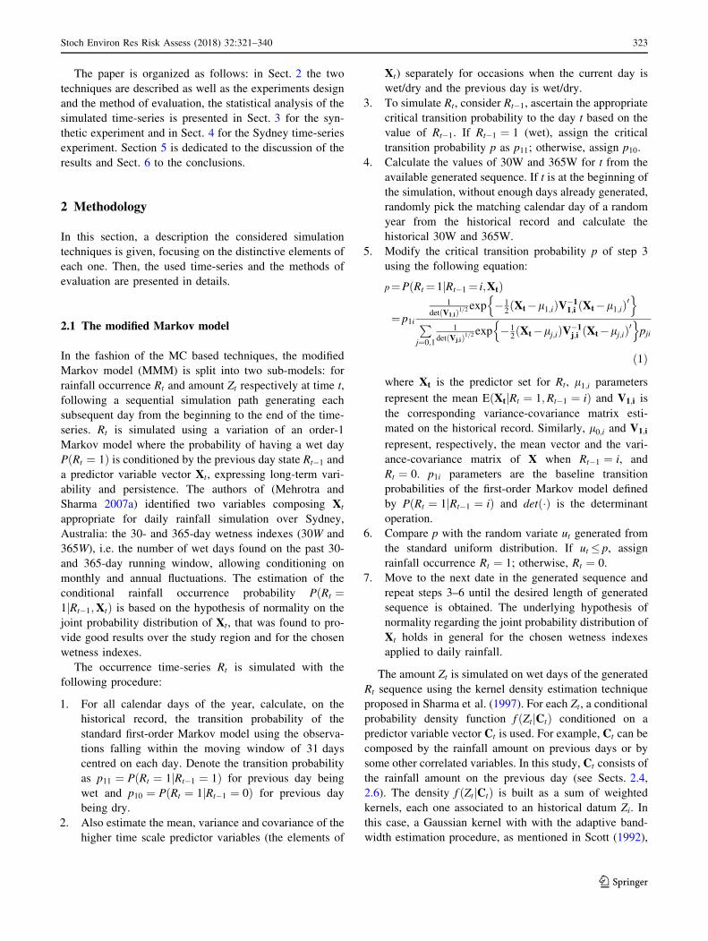
Table 1 Summary of the training data sets and auxiliary variables used in the setup of the two algorithms
Group Training data
amount (days)
Number of data
sets used
Realizations
per data set
MMM setup DS setup
1 1 million 1 (reference) 10 Xt = [30W, 365W], Ct ¼ Zt�1 365W, dw, rainfall
2 10,000 3000 1 Xt ¼ ½30W ; 365W �, Ct ¼ Zt�1 365W, dw, rainfall
3 1000 3000 1 Xt ¼ ½30W ; 365W �, Ct ¼ Zt�1 365W, dw, rainfall
4 100 3000 1 Xt ¼ 30W , Ct ¼ Zt�1 30W, dw, rainfall
The auxiliary variables listed are: the 30- and 365-day wetness indexes (30W and 365W), the previous day simulated rainfall amount Zt�1, the
dry/wet sequence (dw), the daily historical rainfall amount (rainfall). In the MMM algorithm, the vectors Xt and Ct condition the rainfall
occurrence and amount simulation respectively
Table 2 The multivariate setup
used with DS in the synthetic
data experiment
Variable R N T
(1) 365W 5000 21 0.05
(2) dw 10 5 0.05
(3) rainfall 5000 21 0.05
The parameters are: amplitude
of the search radius R (days),
maximum number of neighbors
considered N (days) and dis-
tance threshold T (-)
326 Stoch Environ Res Risk Assess (2018) 32:321–340
123

that Ut presents two regimes with a large variability in their
spell duration and a different time dependence structure.
To contain the computational burden, the following ele-
ments of l are arbitrarily defined: l4 ¼ 1, l6 ¼ 0:51,
l7 ¼ 0:45, l8 ¼ 0:64, l9 ¼ 0:65, while the others are
numerically calibrated to minimize the following objective
function:
where ZA and ZB are the portions of Ut belonging to the
regime A and B respectively, acð�Þ is the lag-1 autocorre-
lation coefficient and �S is the mean length of the time-
series segments belonging to one regime. According to
Eq. 7, low values of the objective function OðlÞ correspondto a reference time-series presenting one or both of the
following features: (1) a large difference between the lag-1
autocorrelation index of the two regimes and (2) a large
difference in the their mean spell length. This allows set-
ting a up the parameters l such that the two regimes present
a sufficient variability in the spell length (creating an
irregular regime alternation) and a sufficiently different
time-dependence structure. Some arbitrary constraints to
the optimization are imposed by accepting a solution only
if 10\�SA\70 and 0\�SB\70, otherwise it is rejected by
putting OðlÞ ¼ 0. This is necessary to avoid an excessive
spell duration, assuring a sufficiently repeated regime
change. Such numerical optimization, constituting a mixed
integer problem, is solved with a genetic algorithm
(Chipperfield et al. 1994), which is often used to find the
minimum of highly non-linear or non-continuous func-
tions. Even if it is not assured that, for a finite time-series
Ut, the algorithm can find the global minimum in a rea-
sonable amount of iterations, it has been observed that, for
this problem, limiting the optimization workflow to 200
iterations is sufficient to obtain an appropriate setup of the
reference model. The resulting parameter values l1 ¼ 6,
l2 ¼ 12, l3 ¼ 95, l5 ¼ 0:30, l10 ¼ 0:31 lead to a similar
wetness level for the two regimes (PðUt ¼ 1Þ � 0:46) but a
different time dependence: regime B presents a higher day-
to-day persistence since Ut is correlated to Ut�1, while, in
regime A, Ut is correlated to lags Ut�6 and Ut�12, resulting
in a more discontinuous dry/wet pattern. Moreover, the
spell duration obtained for both regimes varies from a few
days to about 1500 days (see Fig. 4). A random sample of
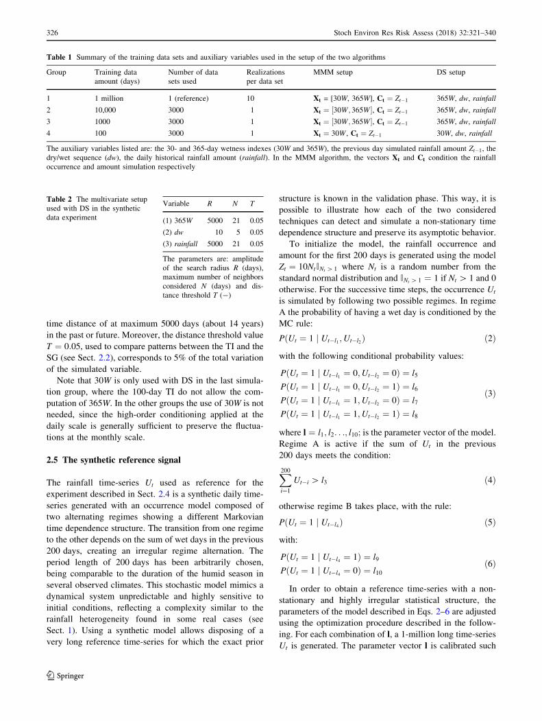
the reference is shown in Fig. 2.
The rainfall amount on wet days of both regimes (his-
togram in Fig. 2) is simulated by randomly sampling the
log-normal distribution lnNð2:74; 0:34Þ, which is fitted on
the starting sequence (first 200 days, then discarded). A
time-series of 1 million days is so obtained by using the
presented model and considered as the reference for the
synthetic test.
2.6 Real data experiment
In this second experiment, the two techniques are compared
on the simulation of the daily rainfall time-series from the
Observatory Hill station, Sydney (Australian Bureau of
Meteorology). This data set has been selected for this study
since the region presents a temperate climate with intense
rainfall events related to extra-tropical cyclones. Moreover,
the influence of the Southern Oscillation (ENSO), causes
extreme droughts and floods, with a highly variable dry/wet
pattern. Finally, the historical record of the chosen station
allows observing with continuity the long-term behavior for
a period of about 150 years. As summarized in Table 3, the
first time-series portion of about 30 years is used as training
data set and initial conditioning data to simulate the
remaining period of about 125 years. An ensemble of 100
realizations is generated with both techniques.
The two algorithms use the canonical setup previously
applied for real rainfall data sets: in addition to the auxiliary
variables used in the previous experiment, MMM includes a
1200-daywetness index (1200W) to condition the simulation
upon long-term fluctuations. Conversely, DS, following the
setup proposed in Oriani et al. (2014), makes use of the 365
moving average (365MA) instead of 365W. This setup also
includes two periodic triangular functions (tr1 and tr2),
based on the day of the year, to describe the annual cycle, and
the 2-day moving sum (2MS) to help respecting the lag-1
autocorrelation. Since tr1 and tr2 are theoretical and known a
priori, they are used in the simulation as conditional data.
2.7 Evaluation
For the synthetic experiment, different statistical indica-
tors, used to analyze the results, describe the overall time-
series as well as the specific statistical signature of the two
regimes. The purpose of studying the regime-specific
statistics allows verifying whether the specific statistical
signature of each regime is detected and preserved in the
OðlÞ ¼ �10jacðZAÞ � acðZBÞj � j�SA � �SBj if 10\�SA\70 and 0\�SB\70
0 otherwise
�ð7Þ
Stoch Environ Res Risk Assess (2018) 32:321–340 327
123
simulation. The probability distribution of daily rainfall
amount on wet days, the annual and decennial amount of
the total signal are compared using qqplots. The two-
regime sequence is then reconstructed inside each simu-
lated time-series with the original criterion used to generate
the reference: the number of wet days over the previous
200 days. This allows separating the two regimes inside the
simulations, to study their alternation and their statistics
separately. A qqplot is used to compare the quantiles of the
two-regime spell length distribution and the dry/wet spell
distribution. To verify the accuracy in the preservation of
the time dependence, the sample autocorrelation function
(ACF) is computed separately for both regimes as well as
on the total signal. Finally, the minimum moving average
(MMA), i.e. the minimum value obtained from the total
daily signal by computing the average on different moving
window sizes, is used to compare the simulation of the
long-term behavior for up to the centennial scale.
For the real data experiment, the same statistics are used,
except for the two-regime analysis, replaced by a group of
indicators describing the annual seasonality, namely: the
monthly probability of occurrence, mean, standard deviation
of the rainfall amount, and the monthly ACF.
3 Synthetic experiment results
The results of the synthetic experiment (described in
Sect. 2.4) are shown in the following and a summary is
given in ‘‘Appendix’’.
3.1 Multiple scale distribution
The comparison with the reference distribution for each
simulation group and technique is shown in Fig. 3. At the
daily scale and using the whole reference as training data
set (1 million-day group), both techniques can accurately
preserve the marginal distribution: the realizations median
shows virtually no bias and the narrow region between the
05–95 % of the simulations indicates very low uncertainty.
Since the reference exhibits a skewed distribution (see
Fig. 2), training data sets smaller than the reference lack
Fig. 2 Rainfall amount
histogram and a random sample
of the synthetic reference signal,
with alternating regimes:
A = lag-6 and -12 Markov
chain and B = lag-1 Markov
chain. The rainfall amount on
all rainy days have been
generated from the same log-
normal probability distribution
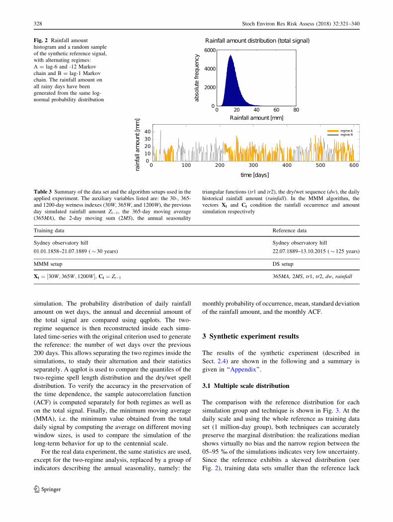
Table 3 Summary of the data set and the algorithm setups used in the
applied experiment. The auxiliary variables listed are: the 30-, 365-
and 1200-day wetness indexes (30W, 365W, and 1200W), the previous
day simulated rainfall amount Zt�1, the 365-day moving average
(365MA), the 2-day moving sum (2MS), the annual seasonality
triangular functions (tr1 and tr2), the dry/wet sequence (dw), the daily
historical rainfall amount (rainfall). In the MMM algorithm, the
vectors Xt and Ct condition the rainfall occurrence and amount
simulation respectively
Training data Reference data
Sydney observatory hill Sydney observatory hill
01.01.1858–21.07.1889 ( 30 years) 22.07.1889–13.10.2015 ( 125 years)
MMM setup DS setup
Xt ¼ ½30W; 365W ; 1200W �, Ct ¼ Zt�1 365MA, 2MS, tr1, tr2, dw, rainfall
328 Stoch Environ Res Risk Assess (2018) 32:321–340
123
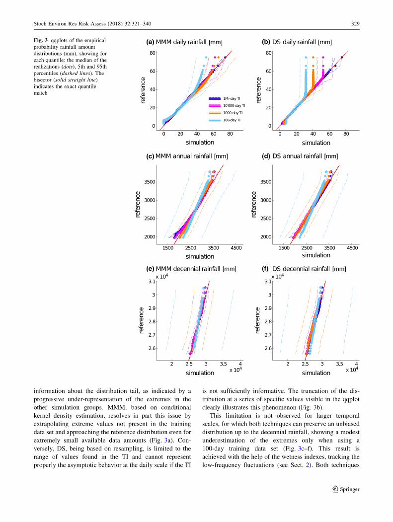
information about the distribution tail, as indicated by a
progressive under-representation of the extremes in the
other simulation groups. MMM, based on conditional
kernel density estimation, resolves in part this issue by
extrapolating extreme values not present in the training
data set and approaching the reference distribution even for
extremely small available data amounts (Fig. 3a). Con-
versely, DS, being based on resampling, is limited to the
range of values found in the TI and cannot represent
properly the asymptotic behavior at the daily scale if the TI
is not sufficiently informative. The truncation of the dis-
tribution at a series of specific values visible in the qqplot
clearly illustrates this phenomenon (Fig. 3b).
This limitation is not observed for larger temporal
scales, for which both techniques can preserve an unbiased
distribution up to the decennial rainfall, showing a modest
underestimation of the extremes only when using a
100-day training data set (Fig. 3c–f). This result is
achieved with the help of the wetness indexes, tracking the
low-frequency fluctuations (see Sect. 2). Both techniques
(a) (b)
(c) (d)
(e) (f)
Fig. 3 qqplots of the empirical
probability rainfall amount
distributions (mm), showing for
each quantile: the median of the
realizations (dots), 5th and 95th
percentiles (dashed lines). The
bisector (solid straight line)
indicates the exact quantile
match
Stoch Environ Res Risk Assess (2018) 32:321–340 329
123

have a comparable performance: we observe only a slight
tendency to overestimate low annual rainfall values by
MMM when using large training data sets. DS is able to re-
aggregate the sampled TI values in different ways and
correctly explore the uncertainty at large scales. Never-
theless, with both techniques, this uncertainty is large when
extremely limited training data sets are used: the 05–95
percentile boundaries of the realizations are very wide
when using 100-day or 1000-day training data groups,
meaning that the used training data sets of this size present
a variable statistical content. This result follows our
expectation: a longer historical record is needed to repre-
sent the large scale variability and better characterize the
uncertainty of the underlying model.
3.2 Regime alternation
As mentioned in Sect. 2.7, the alternation between regimes
A and B is reconstructed inside the generated time-series and
the spell length distribution of each one is shown in Fig. 4.
Even if the reference model is calibrated to assure a con-
tinuous regime alternation, the very skewed spell distribu-
tion still suggests an irregular behavior, with a maximum
spell duration up to about 1500 days for both regimes. The
region delimited by the 05–95 % of the simulations
indicates that the uncertainty increases when reducing the
amount of training data. The 100-day group constitutes the
degenerate case for which the regime transition rule, based
on the 200-day wetness index, is not observable and the
regime alternation cannot be exhaustively represented. In
fact, the 05–95 percentile boundaries (not visible for this
group) correspond to null and infinite spell duration
respectively, meaning that the whole generated time-series
belongs to one single regime. For large training data sets (1
million- and 10,000-day groups) the distribution is preserved
fairly well by both techniques, with a modest under-repre-
sentation of the very upper quantiles for regime A (Fig. 4a,
b). The main difference in their performance is observed in
the 1000-day group, where MMM shows a negative bias
larger than the one obtained in the 100-day group (Fig. 4a, c).
This may indicate that a larger data set is needed to calibrate
the parameters of MMM using the 30- and 365-day wetness
indexes. On the contrary, using the 30-day wetness index
only and a 100-day training data set results in a smaller bias
but larger uncertainty. Representativeness of the training
data set plays again a fundamental role: since no information
about the irregular regime alternation is contained in the
prior structure of both simulation techniques, the distribution
is simulated accurately only when the training data set con-
tains a sufficient repetition of the two-regime transition.
(a) (b)
(c) (d)
Fig. 4 qqplots of the two
regime spell-length distributions
(days) for each simulation group
(different colors), showing for
each quantile: the median of the
realizations (dots), 5th and 95th
percentiles (dashed lines). The
bisector (solid straight line)
indicates the exact quantile
match
330 Stoch Environ Res Risk Assess (2018) 32:321–340
123

3.3 Time dependence structure
The specific short-term time dependence structure of the
total signal as well as the two separate regimes are ana-
lyzed using the sample autocorrelation function (ACF,
Fig. 5). According to its occurrence model, the reference
signal shows a distinctive autocorrelation level (red line)
for lags 6 and 12 in regime A and for lag 1 in regime B,
with the total signal presenting a mixture of both.
The two simulation techniques show different behav-
iors: on the total signal, MMM simulates the lag-1
dependence correctly, but does not preserve the lag-6 and
lag-12 autocorrelation, with a subsequent underestimation
of the persistence (Fig. 5a). This is due to the fact that only
the lag-1 dependence is considered in the MMM occur-
rence model. For this reason, the model is weak to any
other time dependence observable in the training data.
Conversely, DS can preserve the whole time dependence
structure with no need for any prior information about it
(Fig. 5b). This is achieved by applying a random simula-
tion path and a variable conditioning pattern composed of
multiple neighbors (see Sect. 2.2). In other words, a vari-
able high-order time dependence is considered during the
simulation, which allows preserving on average the auto-
correlation at any lags. The advantage of this feature is that
complex non-linear time dependencies are simulated more
easily than using a parametric technique. Note that, for
highly autocorrelated signals, the autocorrelation is not
(a) (b)
(c) (d)
(e) (f)
Fig. 5 Sample ACF of the total
signal and the two regimes for
each simulation group (different
colors). Median of the
realizations (solid lines), 5th
and 95th percentiles (dashed
lines). The red line indicates the
reference
Stoch Environ Res Risk Assess (2018) 32:321–340 331
123
exactly preserved using DS. Even with the most appro-
priate setup, the resampling process adds a small noise to
the data, which is detectable on very smooth signals and
may need a post-processing treatment. In case of daily
rainfall this effect is negligible since the signal presents a
very low autocorrelation.
Both techniques fail in simulating the time dependence
for the two separate regimes. In particular, MMM always
preserves the lag-1 autocorrelation estimated from the total
training data set (Fig. 5c, e) and DS does the same with the
overall dependence structure (Fig. 5d, f). Thismeans that the
non-stationary time dependence linked to the regime alter-
nation cannot be automatically captured and preserved in the
simulation. Designing an ad-hoc model structure based on
the analysis of the training data set is therefore necessary
with both techniques in order to correctly simulate this fea-
ture. For example, information about the irregular regime
alternation can be incorporated in the DS setup using a dis-
crete auxiliary variable as it is done with the dry/wet
sequence (see Sect. 2.2). The mentioned variable would be
simulated together with the rainfall helping the simulation of
the two-regime alternation. Conversely, using a parametric
approach like MMM, a regime switch could be accommo-
dated in theMC structure as it has been done for the reference
signal generation (see Sect. 2.5). In both cases, the main
point is to catch the relevant non-stationary features from the
available data in a preliminary analysis, which may not be
straightforward in case of highly irregular fluctuations.
3.4 Dry/wet pattern and long-term behavior
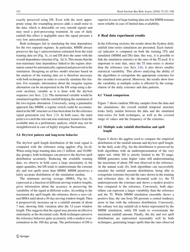
The dry/wet spell length distribution of the total signal is
compared with the reference using qqplots (Fig. 6a–d).
When using large training data sets (1 million- and 10,000-
day groups), both techniques can preserve the dry/wet spell
distribution accurately. Reducing the available training
data, we observe in both cases a large uncertainty in the
upper quantiles, but DS tends to underestimate the extreme
dry and wet spells more than MMM. MMM preserves a
fairly accurate distribution of the simulation median.
The minimum moving average (MMA, Fig. 6e, f),
expressed as a function of different moving window lengths,
gives information about the accuracy in preserving the
variability of the signal at different scales. According to the
maximum dry spell length, the reference shows a zero-val-
uedMMAuntil about a 30-daymovingwindow length. Then
it progressively increases up to a rainfall amount of about
7 mm, showing little variation after the 12-years window
length. This suggests that the signal may present an effective
stationarity at the decennial scale. Both techniques preserve
the reference behavior quite accurately with a modest over-
estimation in the 100-day group. The performance of DS is
superior in case of large training data sets butMMM remains
more reliable in case of limited data availability.
4 Real data experiment results
In the following sections, the results about the Sydney daily
rainfall time-series simulation are presented. Each statisti-
cal indicator is computed on both the training (TI) and
simulated (MMM and DS) data: this way, it is possible to
link the simulation statistics to the ones of the TI used. It is
important to note that, since the TI time-series is shorter
than the reference (see Sect. 2.6), it also shows smaller
statistical variability. This allows analyzing the ability of
the algorithms to extrapolate the appropriate extremes for
the simulated time period. Moreover, the results show how
the variability at multiple scales is affected by the extrap-
olation of the daily extremes and data patterns.
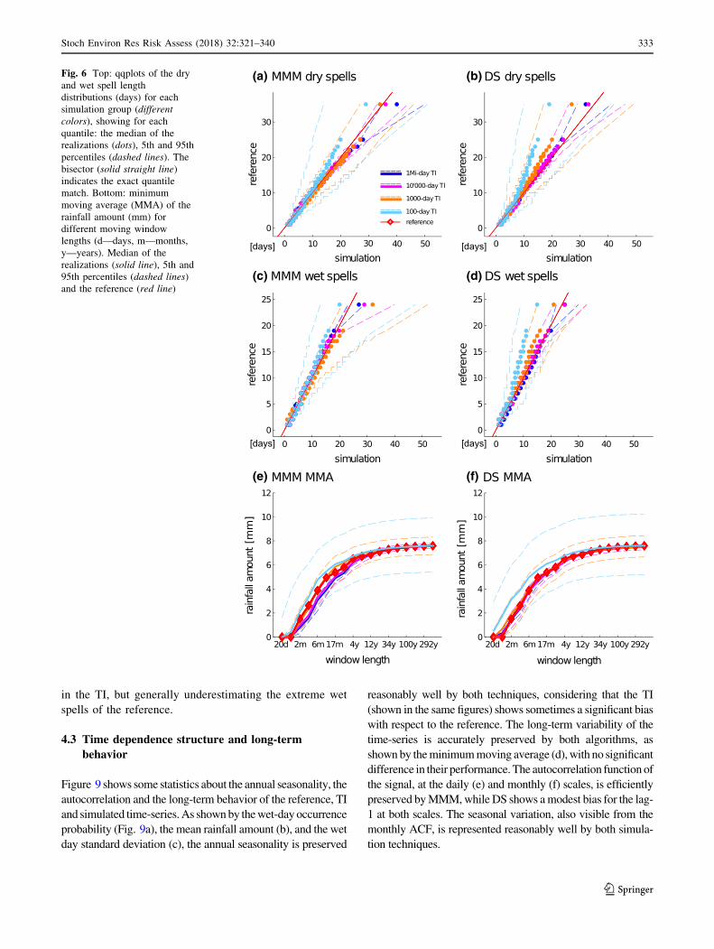
4.1 Visual comparison
Figure 7 shows random 500-day samples from the data and
the simulations: the overall rainfall temporal structure
looks fairly similar between the data and the simulated
time-series for both techniques, as well as the covered
range of values and the frequency of the extremes.
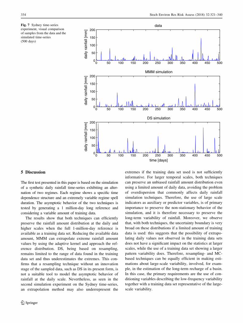
4.2 Multiple scale rainfall distribution and spell
length
Figure 8 shows the qqplots used to compare the empirical
distribution of the rainfall amount and dry/wet spell length.
At the daily scale (Fig. 8a) the distribution is preserved by
both algorithms with an underrepresentation of the very
upper tail: while DS is strictly limited to the TI range,
MMM generates some higher value still underestimating
the maximum of about 300 mm observed in the reference.
At the annual scale (b), both algorithms can successfully
simulate the rainfall amount distribution, being able to
extrapolate extremes beyond the ones shown in the training
and reference data. At the decennial scale (c), the TI
underrepresents the extremes and shows a modest positive
bias compared to the reference. Conversely, both algo-
rithms can represent a larger variability than the reference
and the TI. While MMM simulation ensemble shows a
positive bias, the one from DS presents a central tendency
more in line with the reference distribution. Conversely,
the solitary wet day rainfall (d) is better represented by the
MMM simulation, while DS tends to overestimate the
maximum rainfall amount. Finally, the dry and wet spell
distributions are represented reasonably well by both
techniques, generating longer spells than the ones observed
332 Stoch Environ Res Risk Assess (2018) 32:321–340
123
in the TI, but generally underestimating the extreme wet
spells of the reference.
4.3 Time dependence structure and long-term
behavior
Figure 9 shows some statistics about the annual seasonality, the
autocorrelation and the long-term behavior of the reference, TI
and simulated time-series.As shownby thewet-day occurrence
probability (Fig. 9a), the mean rainfall amount (b), and the wet
day standard deviation (c), the annual seasonality is preserved
reasonably well by both techniques, considering that the TI
(shown in the same figures) shows sometimes a significant bias
with respect to the reference. The long-term variability of the
time-series is accurately preserved by both algorithms, as
shownby theminimummoving average (d),with no significant
difference in their performance.The autocorrelation functionof
the signal, at the daily (e) and monthly (f) scales, is efficiently
preserved byMMM,whileDS shows amodest bias for the lag-
1 at both scales. The seasonal variation, also visible from the
monthly ACF, is represented reasonably well by both simula-
tion techniques.
(a) (b)
(c) (d)
(e) (f)
Fig. 6 Top: qqplots of the dry
and wet spell length
distributions (days) for each
simulation group (different
colors), showing for each
quantile: the median of the
realizations (dots), 5th and 95th
percentiles (dashed lines). The
bisector (solid straight line)
indicates the exact quantile
match. Bottom: minimum
moving average (MMA) of the
rainfall amount (mm) for
different moving window
lengths (d—days, m—months,
y—years). Median of the
realizations (solid line), 5th and
95th percentiles (dashed lines)
and the reference (red line)
Stoch Environ Res Risk Assess (2018) 32:321–340 333
123
5 Discussion
The first test presented in this paper is based on the simulation
of a synthetic daily rainfall time-series exhibiting an alter-
nation of two regimes. Each regime shows a specific time
dependence structure and an extremely variable regime spell
duration. The asymptotic behavior of the two techniques is
tested by generating a 1 million-day long reference and
considering a variable amount of training data.
The results show that both techniques can efficiently
preserve the rainfall amount distribution at the daily and
higher scales when the full 1-million-day reference is
available as a training data set. Reducing the available data
amount, MMM can extrapolate extreme rainfall amount
values by using the adaptive kernel and approach the ref-
erence distribution. DS, being based on resampling,
remains limited to the range of data found in the training
data set and thus underestimates the extremes. This con-
firms that a resampling technique without an innovation
stage of the sampled data, such as DS in its present form, is
not a suitable tool to model the asymptotic behavior of
rainfall at the daily scale. Nevertheless, as seen in the
second simulation experiment on the Sydney time-series,
an extrapolation method may also underrepresent the
extremes if the training data set used is not sufficiently
informative. For larger temporal scales, both techniques
can preserve an unbiased rainfall amount distribution even
using a limited amount of daily data, avoiding the problem
of overdispersion that commonly affects daily rainfall
simulation techniques. Therefore, the use of large scale
indicators as auxiliary or predictor variables, is of primary
importance to preserve the non-stationary behavior of the
simulation, and it is therefore necessary to preserve the
long-term variability of rainfall. Moreover, we observe
that, with both techniques, the uncertainty boundary is very
broad on these distributions if a limited amount of training
data is used: this suggests that the possibility of extrapo-
lating daily values not observed in the training data sets
does not have a significant impact on the statistics at larger
scales, while the use of a training data set showing a larger
pattern variability does. Therefore, resampling- and MC-
based techniques can be equally efficient in making esti-
mations about large-scale variability, involved, for exam-
ple, in the estimation of the long-term recharge of a basin.
In this case, the primary requirements are the use of con-
ditioning variables describing the low-frequency variability
together with a training data set representative of the large-
scale variability.
0 50 100 150 200 250 300 350 400 450 5000
50
100
150
200
daily
rai
nfal
l [m
m]
data
0 50 100 150 200 250 300 350 400 450 5000
50
100
150
200
daily
rai
nfal
l [m
m]
MMM simulation
0 50 100 150 200 250 300 350 400 450 5000
50
100
150
200
time [days]
daily
rai
nfal
l [m
m]
DS simulation
Fig. 7 Sydney time-series
experiment, visual comparison
of samples from the data and the
simulated time-series
(500 days)
334 Stoch Environ Res Risk Assess (2018) 32:321–340
123

The highly irregular two-regime alternation of the syn-
thetic reference signal is preserved fairly well by both
techniques using a large training data set. The specific
high-order temporal correlation contained in the whole
signal is automatically captured and preserved by DS,
while MMM underestimates the persistence since it is
limited to the lag-1 time conditioning contained in its prior
structure. These results confirm that, using a Markov-chain
based approach, a preliminary analysis is necessary to
include the salient high-order time dependence features in
the prior structure of the model. The autocorrelation
function of the two separate regimes, showing a different
time dependence signature, is not correctly preserved by
either the approaches, meaning that information about this
kind of non-stationarity should first be detected then
explicitly incorporated in the prior structure of both mod-
els. In the case of MMM, this should be is possible by
implementing a regime switch in the Markov-chain con-
ditioning structure. Using DS, a regime indicator can be
calculated on the training data set and jointly simulated
with the rainfall signal.
Finally, the dry/wet spell distribution and the minimum
moving average of the rainfall amount confirms the higher
accuracy of DS in simulating long wet periods and the
multiple-scale features when a sufficient training data set is
available. MMM is more reliable in case of scarce data
availability, where DS underestimates the length of both
the dry and wet extreme spells.
The second and last test sees the simulation of a daily
rainfall time-series from Sydney using the initial recorded
30 years as training data set and simulating the longer
remaining portion of about 125 years. The results show a
similar performance of the techniques with respect to the
first experiment, underlining the importance of a repre-
sentative training data set, despite the capability of
extrapolation of the techniques at different scales. As seen
in the results, an exiguous training data set with respect to
the simulated period may not only underrepresent the
(a) (b)
(c) (d)
(e) (f)
Fig. 8 Sydney time-series
experiment results, qqplots of
different indicators, including:
daily (a), annual (b), 10-year(c), solitary wet-day (d) rainfallamount, wet (e) and dry (f) spelllength (days). For each
indicator, DS and MMM
simulations together with the
training data set distributions
are compared with the reference
one. For DS and MMM, the
median of the realizations (solid
line) is shown as well as the 5th
and 95th percentiles (dashed
lines)
Stoch Environ Res Risk Assess (2018) 32:321–340 335
123

extremes, but it may also present a significant bias in some
central tendency indicators, for example the ones regarding
the annual seasonality.
6 Conclusions
In this paper, we investigate the performance of some
advanced statistical strategies used to simulate the complex
structure of rainfall at multiple scales. This is done by
comparing two recent techniques for daily rainfall simu-
lation: the Markov-chain based modified Markov model
(MMM) and the direct sampling technique (DS) belonging
to the multiple-point statistics family. The two algorithms
use the same type of information under the form of vari-
ables computed from the rainfall amount, namely: the
rainfall state (dry or wet) and the wetness indexes, i.e. the
number of wet days in the past, informing about low-fre-
quency fluctuations. MMM is a semi-parametric model
where the rainfall state generation is conditioned on a fixed
order-1 time dependence and low-frequency fluctuations.
The rainfall amount is generated using an order-1 condi-
tional kernel density estimation (the adaptive kernel). This
way, non-stationarity is introduced in the parameters of
both the occurrence and amount models allowing the
preservation of the essential small- and large-scale char-
acteristics of rainfall. Conversely, DS is a fully non-para-
metric resampling technique based on a pattern-similarity
rule. Using a random simulation path and a variable con-
ditioning pattern, DS simulates the same type of patterns
found in the training data set at multiple scales. Conse-
quently, high-order statistics contained in the training data
are indirectly preserved in the simulations without the need
for a complex parameterization.
The results presented in this paper suggest a series of
elements that can be incorporated in a daily simulation
approach to preserve, at a reasonable level, the complexity
of the rainfall variability:
(a) (b)
(c) (d)
(e) (f)
Fig. 9 Sydney time-series
applied experiment: monthly
wet-day probability of rainfall
occurrence (a), mean rainfall
(b), standard deviation (c),minimum moving average (d),daily (e) and monthly (f) rainfallsample autocorrelation. For
each indicator, DS and MMM
simulation ensembles (boxplots)
are compared to the training and
reference data sets (solid lines).
For d, the median of the
realizations (solid line) is shown
as well as the 5th and 95th
percentiles (dashed lines)
336 Stoch Environ Res Risk Assess (2018) 32:321–340
123

1. The daily variability in both the dry/wet structure and
rainfall amount can be better preserved with an
adaptive kernel technique when a scarce training data
set is used, while a non-parametric resampling strategy
is more suitable when a rich training data set is
available. Ideally and in both cases, the recommended
training data set length should encompass a longer
period than the one simulated to represent long
recurrence time events;
2. The extrapolation of values not observed in the
training data set is of primary importance to correctly
represent the extremes at the daily scale, while it is not
fundamental to preserve the variability at higher scale,
for example to estimate the long-term recharge of a
basin—in these cases, a technique purely based on
resampling at the daily scale may suit the purpose;
3. The use of low-frequency covariates of daily rainfall is
an efficient strategy to preserve the long-term behav-
ior—a Markov-chain based as well as a resampling
technique can accommodate the use of these variables;
4. To preserve a complex time dependence structure, a
resampling procedure considering a variable time
dependence, as it has been implemented in DS, is
more convenient than a MC-model, since it is adaptive
to different data patterns with a simple parameteriza-
tion. Nevertheless, this approach entirely relies on the
training data set. Therefore, in case of scarce training
data, a parametric technique taking into account only
the low-order dependency may be more appropriate,
since the high-order statistics, like the long-term
behavior of rainfall, are not observable in the data;
5. A simulation strategy accommodating a variable time-
dependence is convenient in case of conditional or
missing data simulation: considering data patterns of
different configuration allows for conditioning data
anywhere in time, simplifying the simulation from the
user-perspective;
6. Non-stationarity, like the presence of different rainfall
regimes, should be investigated a priori and included in
the structure of the algorithm, e.g. under form of
conditioning variables.
To incorporate all these features in a unified framework,
future research could focus on the development of a semi-
parametric or kernel based amount model inside the DS
framework to perturb the sampled historical values. This
idea has been already proposed for k-nearest neighbor
resampling techniques (Lall and Sharma 1996; Rajagopa-
lan and Lall 1999) and applied to some stochastic hydro-
logical models of the same family: inspired by traditional
autoregressive models, they consider the non-linear
regression mðHiÞ to describe the relationship between the
training data Zi and a predictor variable vector Hi. The
simulated value Zt ¼ mðHtÞ þ et is the sum of the deter-
ministic conditional mean mðHtÞ and an innovation term et,
generated by sampling from the local residuals of mðHtÞ(Prairie et al. 2006) or calibrating a random noise on them
(Singhrattna et al. 2005; Sharif and Burn 2007). These
works show that the introduction of an innovation term is a
promising path to increase the prediction skills of resam-
pling techniques. Moreover, the parametric framework of
these algorithms present a fixed time-dependence condi-
tioning, which, on the contrary, is variable in the non-
parametric approach of DS. For these reasons, the devel-
opment of a perturbation stage of the sampled values in the
direct sampling framework may lead to an improved
model. Finally, future simulation techniques may also
include a variable describing the non-stationarity in the
training data set. This could influence the variation of MC
parameters through time or guide a resampling procedure
in generating non-stationary data patterns.
Acknowledgements This research was funded by the Swiss National
Science Foundation (Project No. 134614) and the National Centre for
Groundwater Research and Training (Australia). We thank Prof.
Geoffrey G.S. Pegram for his review and suggested modifications
prior to the submission of the final version of this paper. The data
used to produce the results of this paper are freely available upon
request to the corresponding author.
Appendix: Summary of the test on synthetic data
As shown in Sect. 3, the two considered algorithms present
a different behavior with respect to various characteristics
of the signal and training data amounts considered. The
relative error D ¼ ðs� rÞ=r (r = reference, s = simula-
tions median) is calculated on a selection of indicators
(Table 4), to summarize the average performance of the
two techniques. Positive values indicate overestimation and
negative ones underestimation: for example DQ95 ¼�0:50 indicates that the 95-th percentile has been under-
estimated by 50%. The chosen error indicators mainly
regard the error in the tail of the considered probability
distributions, since the central and lower part are generally
preserved by both algorithms.
In accordance with the results shown in previous pub-
lications (Mehrotra and Sharma 2007a, b; Oriani et al.
2014), it is shown here that both techniques can generate
replicates of the same size as the training data set pre-
serving the rainfall variability at multiple scales. The error
on the tail of the distribution (DQ99 and DQ100) is in fact
very low for the daily rainfall amount up to the decennial
scale in the 1-million simulation group. Reducing the
available amount of data, MMM can extrapolate extremes
by using a conditional kernel smoothing technique, while
DS remains limited to the range of data found in the TI. At
Stoch Environ Res Risk Assess (2018) 32:321–340 337
123
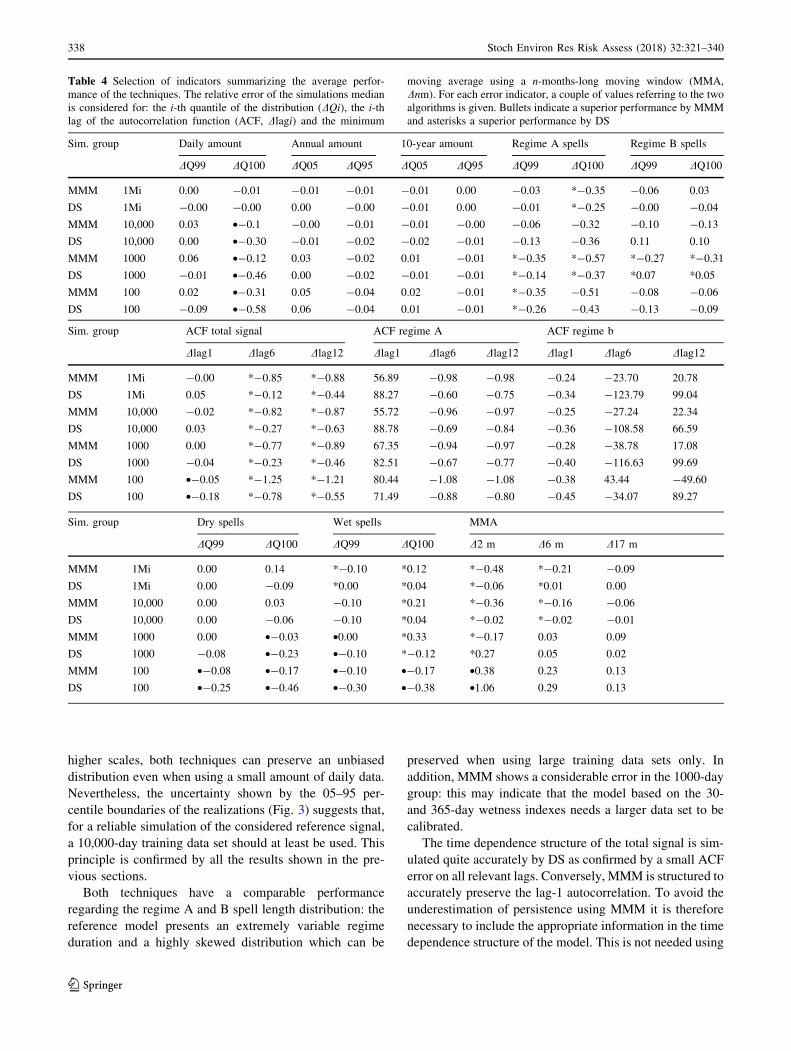
higher scales, both techniques can preserve an unbiased
distribution even when using a small amount of daily data.
Nevertheless, the uncertainty shown by the 05–95 per-
centile boundaries of the realizations (Fig. 3) suggests that,
for a reliable simulation of the considered reference signal,
a 10,000-day training data set should at least be used. This
principle is confirmed by all the results shown in the pre-
vious sections.
Both techniques have a comparable performance
regarding the regime A and B spell length distribution: the
reference model presents an extremely variable regime
duration and a highly skewed distribution which can be
preserved when using large training data sets only. In
addition, MMM shows a considerable error in the 1000-day
group: this may indicate that the model based on the 30-
and 365-day wetness indexes needs a larger data set to be
calibrated.
The time dependence structure of the total signal is sim-
ulated quite accurately by DS as confirmed by a small ACF
error on all relevant lags. Conversely, MMM is structured to
accurately preserve the lag-1 autocorrelation. To avoid the
underestimation of persistence using MMM it is therefore
necessary to include the appropriate information in the time
dependence structure of the model. This is not needed using
Table 4 Selection of indicators summarizing the average perfor-
mance of the techniques. The relative error of the simulations median
is considered for: the i-th quantile of the distribution (DQi), the i-th
lag of the autocorrelation function (ACF, Dlagi) and the minimum
moving average using a n-months-long moving window (MMA,
Dnm). For each error indicator, a couple of values referring to the two
algorithms is given. Bullets indicate a superior performance by MMM
and asterisks a superior performance by DS
Sim. group Daily amount Annual amount 10-year amount Regime A spells Regime B spells
DQ99 DQ100 DQ05 DQ95 DQ05 DQ95 DQ99 DQ100 DQ99 DQ100
MMM 1Mi 0.00 -0.01 -0.01 -0.01 -0.01 0.00 -0.03 *-0.35 -0.06 0.03
DS 1Mi -0.00 -0.00 0.00 -0.00 -0.01 0.00 -0.01 *-0.25 -0.00 -0.04
MMM 10,000 0.03 •-0.1 -0.00 -0.01 -0.01 -0.00 -0.06 -0.32 -0.10 -0.13
DS 10,000 0.00 •-0.30 -0.01 -0.02 -0.02 -0.01 -0.13 -0.36 0.11 0.10
MMM 1000 0.06 •-0.12 0.03 -0.02 0.01 -0.01 *-0.35 *-0.57 *-0.27 *-0.31
DS 1000 -0.01 •-0.46 0.00 -0.02 -0.01 -0.01 *-0.14 *-0.37 *0.07 *0.05
MMM 100 0.02 •-0.31 0.05 -0.04 0.02 -0.01 *-0.35 -0.51 -0.08 -0.06
DS 100 -0.09 •-0.58 0.06 -0.04 0.01 -0.01 *-0.26 -0.43 -0.13 -0.09
Sim. group ACF total signal ACF regime A ACF regime b
Dlag1 Dlag6 Dlag12 Dlag1 Dlag6 Dlag12 Dlag1 Dlag6 Dlag12
MMM 1Mi -0.00 *-0.85 *-0.88 56.89 -0.98 -0.98 -0.24 -23.70 20.78
DS 1Mi 0.05 *-0.12 *-0.44 88.27 -0.60 -0.75 -0.34 -123.79 99.04
MMM 10,000 -0.02 *-0.82 *-0.87 55.72 -0.96 -0.97 -0.25 -27.24 22.34
DS 10,000 0.03 *-0.27 *-0.63 88.78 -0.69 -0.84 -0.36 -108.58 66.59
MMM 1000 0.00 *-0.77 *-0.89 67.35 -0.94 -0.97 -0.28 -38.78 17.08
DS 1000 -0.04 *-0.23 *-0.46 82.51 -0.67 -0.77 -0.40 -116.63 99.69
MMM 100 •-0.05 *-1.25 *-1.21 80.44 -1.08 -1.08 -0.38 43.44 -49.60
DS 100 •-0.18 *-0.78 *-0.55 71.49 -0.88 -0.80 -0.45 -34.07 89.27
Sim. group Dry spells Wet spells MMA
DQ99 DQ100 DQ99 DQ100 D2 m D6 m D17 m
MMM 1Mi 0.00 0.14 *-0.10 *0.12 *-0.48 *-0.21 -0.09
DS 1Mi 0.00 -0.09 *0.00 *0.04 *-0.06 *0.01 0.00
MMM 10,000 0.00 0.03 -0.10 *0.21 *-0.36 *-0.16 -0.06
DS 10,000 0.00 -0.06 -0.10 *0.04 *-0.02 *-0.02 -0.01
MMM 1000 0.00 •-0.03 •0.00 *0.33 *-0.17 0.03 0.09
DS 1000 -0.08 •-0.23 •-0.10 *-0.12 *0.27 0.05 0.02
MMM 100 •-0.08 •-0.17 •-0.10 •-0.17 •0.38 0.23 0.13
DS 100 •-0.25 •-0.46 •-0.30 •-0.38 •1.06 0.29 0.13
338 Stoch Environ Res Risk Assess (2018) 32:321–340
123

DS since it can automatically simulate complex time
dependence by generating multiscale patterns similar to the
ones found in the training data set. Large errors shown by
both techniques in theACF of the separate regimes are due to
their inability to capture the non-stationarity of the two-
regime alternation in absence of prior information about it.
Finally, the error on the dry/wet spell length distribu-
tions and on the minimum moving average confirms the
same tendency: we observe a better performance of DS
when sufficient training data are available. MMM is more
reliable in case of scarce data availability.
References
Andrade C, Trigo RM, Freitas MC, Gallego MC, Borges P, Ramos
AM (2008) Comparing historic records of storm frequency and
the north atlantic oscillation (nao) chronology for the azores
region. Holocene 18(5):745–754. doi:10.1177/095968360809
1794
Arpat G, Caers J (2007) Conditional simulation with patterns. Math
Geol 39(2):177–203
Bardossy A, Plate EJ (1992) Space–time model for daily rainfall
using atmospheric circulation patterns. Water Resour Res
28(5):1247–1259. doi:10.1029/91WR02589
Basu S, Andharia HI (1992) The chaotic time-series of indian
monsoon rainfall and its prediction. Proc Indian Acad Sci Earth
Planet Sci 101(1):27–34
Briggs WM, Wilks DS (1996) Estimating monthly and seasonal
distributions of temperature and precipitation using the new cpc
long-range forecasts. J Clim 9(4):818–826. doi:10.1175/1520-
0442(1996)009\0818:EMASDO[2.0.CO;2
Buishand T (1978) Some remarks on the use of daily rainfall models.
J Hydrol 36(3–4):295–308
Buishand TA, Brandsma T (2001) Multisite simulation of daily
precipitation and temperature in the rhine basin by nearest-
neighbor resampling. Water Resour Res 37(11):2761–2776.
doi:10.1029/2001WR000291
Chipperfield A, Fleming P, Fonseca C (1994) Genetic algorithm tools
for control systems engineering. In: Proceedings of adaptive
computing in engineering design and control. Citeseer,
pp 128–133
Chou C, Tu JY, Yu JY (2003) Interannual variability of the western
north pacific summer monsoon: differences between enso and
non-enso years. J Clim 16(13):2275–2287. doi:10.1175/2761.1
Elsanabary MH, Gan TY, Mwale D (2014) Application of wavelet
empirical orthogonal function analysis to investigate the non-
stationary character of ethiopian rainfall and its teleconnection to
nonstationary global sea surface temperature variations for
1900–1998. Int J Climatol 34(6):1798–1813. doi:10.1002/joc.
3802
Feng X, ChangZheng L (2008) The influence of moderate enso on
summer rainfall in eastern china and its comparison with strong
enso. Chin Sci Bull 53(5):791–800. doi:10.1007/s11434-008-
0002-5
Gabriel K, Neumann J (1962) A markov chain model for daily rainfall
occurrence at tel aviv. Q J R Meteorol Soc 88(375):90–95
Garcia-Barron L, Aguilar M, Sousa A (2011) Evolution of annual
rainfall irregularity in the southwest of the iberian peninsula.
Theor Appl Climatol 103(1–2):13–26. doi:10.1007/s00704-010-
0280-0
Guardiano F, Srivastava R (1993) Multivariate geostatistics: beyond
bivariate moments. Geostat Troia 1:133–144
Harrold TI, Sharma A, Sheather SJ (2003a) A nonparametric model
for stochastic generation of daily rainfall amounts. Water Resour
Res 39(12):1343. doi:10.1029/2003WR002570
Harrold TI, Sharma A, Sheather SJ (2003b) A nonparametric model
for stochastic generation of daily rainfall occurrence. Water
Resour Res 39(10):1300. doi:10.1029/2003WR002182
Hay LE, Mccabe GJ, Wolock DM, Ayers MA (1991) Simulation of
precipitation by weather type analysis. Water Resour Res
27(4):493–501. doi:10.1029/90WR02650
Honarkhah M, Caers J (2010) Stochastic simulation of patterns using
distance-based pattern modeling. Math Geosci 42(5):487–517
Hughes J, Guttorp P (1994) A class of stochastic models for relating
synoptic atmospheric patterns to regional hydrologic phenom-
ena. Water Resour Res 30(5):1535–1546
Hughes J, Guttorp P, Charles S (1999) A non-homogeneous hidden
markov model for precipitation occurrence. J Roy Stat Soc: Ser
C (Appl Stat) 48(1):15–30
Jayawardena AW, Lai FZ (1994) Analysis and prediction of chaos in
rainfall and stream-flow time-series. J Hydrol 153(1–4):23–52.
doi:10.1016/0022-1694(94)90185-6
Jones PG, Thornton PK (1997) Spatial and temporal variability of
rainfall related to a third-order markov model. Agric For
Meteorol 86(1–2):127–138. doi:10.1016/S0168-1923(96)02399-
4
Jothiprakash V, Fathima TA (2013) Chaotic analysis of daily rainfall
series in koyna reservoir catchment area, india. Stoch Env Res
Risk Assess 27(6):1371–1381. doi:10.1007/s00477-012-0673-y
Katz R, Parlange M (1998) Overdispersion phenomenon in stochastic
modeling of precipitation. J Clim 11(4):591–601
Katz RW, Parlange MB (1993) Effects of an index of atmospheric
circulation on stochastic properties of precipitation. Water
Resour Res 29(7):2335–2344. doi:10.1029/93WR00569
Katz RW, Zheng XG (1999) Mixture model for overdispersion of
precipitation. J Clim 12(8):2528–2537. doi:10.1175/1520-
0442(1999)012\2528:MMFOOP[2.0.CO;2
Kelley OA (2014) Where the least rainfall occurs in the sahara desert,
the trmm radar reveals a different pattern of rainfall each season.
J Clim 27(18):6919–6939. doi:10.1175/JCLI-D-14-00145.1
Khan S, Ganguly AR, Saigal S (2005) Detection and predictive
modeling of chaos in finite hydrological time series. Nonlinear
Process Geophys 12(1):41–53
Kiely G, Albertson JD, Parlange MB, Katz RW (1998) Conditioning
stochastic properties of daily precipitation on indices of atmo-
spheric circulation. Meteorol Appl 5(1):75–87. doi:10.1017/
S1350482798000656
Lall U, Sharma A (1996) A nearest neighbor bootstrap for resampling
hydrologic time series. Water Resour Res 32(3):679–693. doi:10.
1029/95WR02966
Mariethoz G, Renard P, Straubhaar J (2010) The direct sampling
method to perform multiple-point geostatistical simulations.
Water Resour Res 46(11):W11,536. doi:10.1029/2008WR00
7621
Mehrotra R, Li JW, Westra S, Sharma A (2015) A programming tool
to generate multi-site daily rainfall using a two-stage semi
parametric model. Environ Model Softw 63:230–239. doi:10.
1016/j.envsoft.2014.10.016
Mehrotra R, Sharma A (2007a) Preserving low-frequency variability
in generated daily rainfall sequences. J Hydrol 345(1–2):102–
120. doi:10.1016/j.jhydrol.2007.08.003
Mehrotra R, Sharma A (2007b) A semi-parametric model for
stochastic generation of multi-site daily rainfall exhibiting low-
frequency variability. J Hydrol 335(1–2):180–193. doi:10.1016/j.
jhydrol.2006.11.011
Stoch Environ Res Risk Assess (2018) 32:321–340 339
123
Millan H, Rodriguez J, Ghanbarian-Alavijeh B, Biondi R, Llerena G
(2011) Temporal complexity of daily precipitation records from
different atmospheric environments: Chaotic and levy stable pa-
rameters. Atmos Res 101(4):879–892. doi:10.1016/j.atmosres.
2011.05.021
Munoz-Diaz D, Rodrigo FS (2003) Effects of the north atlantic
oscillation on the probability for climatic categories of local
monthly rainfall in southern spain. Int J Climatol 23(4):381–397.
doi:10.1002/joc.886
Oriani F, Straubhaar J, Renard P, Mariethoz G (2014) Simulation of
rainfall time series from different climatic regions using the
direct sampling technique. Hydrol Earth Syst Sci 18(8):3015–
3031. doi: 10.5194/hess-18-3015-2014http://www.hydrol-earth-
syst-sci.net/18/3015/2014/
Prairie JR, Rajagopalan B, Fulp TJ, Zagona EA (2006) Modified k-nn
model for stochastic streamflow simulation. J Hydrol Eng
11(4):371–378. doi:10.1061/(ASCE)1084-0699(2006)11:4(371)
Rajagopalan B, Lall U (1999) A k-nearest-neighhor simulator for
daily precipitation and other weather variables. Water Resour
Res 35(10):3089–3101. doi:10.1029/1999WR900028
Schertzer D, Tchiguirinskaia I, Lovejoy S, Hubert P, Bendjoudi H,
Larcheveque M (2002) Discussion of ‘‘evidence of chaos in the
rainfall-runoff process’’—which chaos in the rainfall-runoff process?
Hydrol Sci J 47(1):139–148. doi:10.1080/02626660209492913
Scott DW (1992) Multivariate density estimation: theory, practice,
and visualization. Wiley, New York
Sharif M, Burn DH (2007) Improved k-nearest neighbor weather
generating model. J Hydrol Eng 12(1):42–51. doi:10.1061/
(ASCE)1084-0699(2007)12:1(42)
Sharma A, Tarboton D, Lall U (1997) Streamflow simulation: a
nonparametric approach. Water Resour Res 33(2):291–308.
doi:10.1029/96WR02839
Singhrattna N, Rajagopalan B, Clark M, Kumar KK (2005) Seasonal
forecasting of thailand summer monsoon rainfall. Int J Climatol
25(5):649–664. doi:10.1002/joc.1144
Sivakumar B, Berndtsson R, Olsson J, Jinno K (2001) Evidence of
chaos in the rainfall-runoff process. Hydrol Sci J 46(1):131–145.
doi:10.1080/02626660109492805
Sivakumar B, Liong S, Liaw C (1998) Evidence of chotic behaviour
in singapore rainfall. JAWRA J Am Water Resour Assoc 34(2):
301–310
Sivakumar B, Woldemeskel FM, Puente CE (2014) Nonlinear
analysis of rainfall variability in australia. Stoch Env Res Risk
Assess 28(1):17–27. doi:10.1007/s00477-013-0689-y
Srikanthan R (2004) Stochastic generation of daily rainfall data using
a nested model. In: 57th Canadian water resources association
annual congress. pp 16–18
Srikanthan R (2005) Stochastic generation of daily rainfall data using
a nested transition probability matrix model. In: 29th hydrology
and water resources symposium: water capital, 20–23 February
2005, Rydges Lakeside, Canberra. Engineers Australia, p 26
Srikanthan R, Pegram GGS (2009) A nested multisite daily rainfall
stochastic generation model. J Hydrol 371(1–4):142–153. doi:10.
1016/j.jhydrol.2009.03.025
Straubhaar J (2011) MPDS technical reference guide. Centre d’hy-
drogeologie et geothermie, University of Neuchatel, Neuenburg
Straubhaar J, Renard P, Mariethoz G (2016) Conditioning multiple-
point statistics simulations to block data. Spat Stat 16:53–71
Straubhaar J, Renard P, Mariethoz G, Froidevaux R, Besson O (2011)
An improved parallel multiple-point algorithm using a list
approach. Math Geosci 43(3):305–328
Strebelle S (2002) Conditional simulation of complex geological
structures using multiple-point statistics. Math Geol 34(1):1–21
Tahmasebi P, Hezarkhani A, Sahimi M (2012) Multiple-point
geostatistical modeling based on the cross-correlation functions.
Comput Geosci 16(3):779–797
Trigo R, Zezere JL, Rodrigues ML, Trigo IF (2005) The influence of
the north atlantic oscillation on rainfall triggering of landslides
near lisbon. Nat Hazards 36(3):331–354. doi:10.1007/s11069-
005-1709-0
Wallis TWR, Griffiths JF (1997) Simulated meteorological input for
agricultural models. Agric For Meteorol 88(1–4):241–258.
doi:10.1016/S0168-1923(97)00035-X
Wang QJ, Nathan RJ (2002) A daily and monthly mixed algorithm for
stochastic generation of rainfall time series. In: Water challenge:
balancing the risks: hydrology and water resources symposium
2002. Institution of Engineers, Australia, p 698
Wilby RL (1998) Modelling low-frequency rainfall events using
airflow indices, weather patterns and frontal frequencies. J Hy-
drol 212(1–4):380–392. doi:10.1016/S0022-1694(98)00218-2
Wilks DS (1989) Conditioning stochastic daily precipitation models
on total monthly precipitation. Water Resour Res 25(6):1429–
1439. doi:10.1029/WR025i006p01429
Wojcik R, McLaughlin D, Konings A, Entekhabi D (2009) Condi-
tioning stochastic rainfall replicates on remote sensing data.
IEEE Trans Geosci Remote Sens 47(8):2436–2449
Woolhiser DA, Keefer TO, Redmond KT (1993) Southern oscillation
effects on daily precipitation in the southwestern united-states.
Water Resour Res 29(4):1287–1295. doi:10.1029/92WR02536
Zanchettin D, Franks SW, Traverso P, Tomasino M (2008) On enso
impacts on european wintertime rainfalls and their modulation by
the nao and the pacific multi-decadal variability described through
the pdo index. Int J Climatol 28(8):995–1006. doi:10.1002/joc.1601
Zhang T, Switzer P, Journel A (2006) Filter-based classification of
training image patterns for spatial simulation. Math Geol
38(1):63–80
340 Stoch Environ Res Risk Assess (2018) 32:321–340
123