simulating evolution and behaviour
TRANSCRIPT
Simulating Evolution and Behaviour
with monkey.py, redqueen.py, relationship.py
Abhranil Das
IISER Kolkata
1 monkey.py
Abstract
The Infinite Monkey Theorem proposes a dumb monkey at a type-writer that takes more than the age of the universe to come up with aShakespearean quote. Creationists equate this monkey with the forceof evolution and thus denounce the theory. This report discusses aprogram emulating a modified monkey which can implement naturalselection and thus generate the desired quote within a few tries.
1.1 Theory
The Infinite Monkey Theorem states that if a monkey sat at a type-writer and started pressing keys at random, it would take him morethan the age of the universe to come up with something like a quotefrom Shakespeare. Creationists immediately grabbed this idea andused it against the theory of evolution. They said that evolution alsotakes place through random mutations, and so is blind and withoutforesight, just as the monkey does not know which phrase he is sup-posed to generate. Thus, the random mutations may be equated tothe random jabs of the monkey at the typewriter. How come, then,could evolutionists claim that complex organs like eyes and nervesand brains could evolve within a tiny fraction of the age of the uni-verse? If a single phrase from Shakespeare cannot be generated by themonkey within the span of the age of the universe, how can we see’products of evolution’ roaming the earth that are far more complexin design than a Shakespearean quote? The creationists said therefore
1

1 monkey.py 2
that these complex biological objects are really the manifestation of in-telligent design. In fact, a program called The Monkey ShakespeareSimulator was written that emulates a large population of monkeys. Ittook 2,737,850 million billion billion billion monkey-years to come upwith:
RUMOUR. Open your ears; 9r"5j5&?OWTY Z0d...Does that mean that evolution as a theory is disproved?Of course not. The key point missing here in the analogy with the
monkey is that there is no natural selection in case of the monkey. Al-though in evolution we have purely random mutations, these muta-tions are preferentially chosen via natural selection, which is not a ran-dom process at all. Every mutation has an associated fitness, whichhelps it to survive. Gradually, therefore, the individuals comprisingthe population become fitter and fitter. In such a situation, it is notuncommon for eyes and brains to evolve within a tiny fraction of theage of the universe.
Therefore, if we modify the program emulating the monkey so thatit now looks at what it has randomly typed and judges its fitness, andthen produces mutated copies of the fittest phrase, then again picksthe fittest etc, we might very well be able to generate a quote by Shake-speare, provided we define that quote beforehand as being the fittestphrase possible.
1.2 Aim
i.) To write a program to emulate the monkey sitting at the type-writer and generating random phrases, but also effecting nat-ural selection.
ii.) To check whether we can generate desired phrases startingfrom a random or a user-defined phrase.
iii.) To generate a fitness v/s generation plot.
1.3 The Program
The Program was written in Python. The program is the following:
1 # ! / usr / b in / python2 import random , commands , Gnuplot3 while True :

1 monkey.py 3
4 s r c = raw_input ( ’ Source phrase of same length as d e s t i n a t i o nphrase ( enter blank f o r random source phrase ) : ’ )
5 dst = raw_input ( ’ Des t ina t ion phrase : ’ )6 d = len ( dst )7 pop = input ( ’ Population s i z e : ’ )8 N = input ( ’ Generation count ( enter 0 to stop at f i r s t s u c c e s s f u l
generat ion ) : ’ )9 c h r s e t = ’ ’ . j o i n ( [ chr ( i ) for i in range ( 3 2 , 1 2 7 ) ] )
10 l = [ ’ ’ ]∗d11 t i t l e = ’ ’12 i f len ( s r c ) <>0:13 l = [ i for i in s r c ]14 t i t l e = s r c15 e lse :16 for i in range ( d ) :17 l [ i ] = random . sample ( [ j for j in c h r s e t ] , 1 ) [ 0 ]18 t i t l e = ’ ’ . j o i n ( l ) + ’ (Random) ’19 t i t l e = ( chr ( 3 9 ) ∗2) . j o i n ( t i t l e . s p l i t ( chr ( 3 9 ) ) )20 lpop = [ [ ’ ’ ]∗d]∗pop21 ppop = lpop [ : ]22 prob = [ ’ ’ ]∗d23 for i in range ( d ) :24 prob [ i ] = f l o a t ( min ( [ abs ( c h r s e t . f ind ( dst [ i ] ) − c h r s e t .
f ind ( l [ i ] ) ) , len ( c h r s e t ) − abs ( c h r s e t . f ind ( dst [ i ] ) −c h r s e t . f ind ( l [ i ] ) ) ] ) ) /( len ( c h r s e t ) /2)
25 psum = [sum( prob ) ]∗pop26 l p l o t = [ ]27 n = 128 i n s t = ’ ’29 f = open ( ’ monkeydata . t x t ’ , ’w’ )30 print >> f , ’ Source : ’ , t i t l e31 print >> f , ’ Des t ina t ion : ’ , dst32 print >> f , ’ Population : ’ , pop33 while True :34 i n s t = ’ ’ . j o i n ( l )35 print >>f , ’\n ’ , n , ’\ t ’ , i n s t , ’\ t ’ , 1 − min (psum) /d , ’\n ’36 l p l o t . append ( s t r ( n ) )37 l p l o t . append ( ’\ t ’ )38 l p l o t . append ( s t r (1 − min (psum) /d ) )39 l p l o t . append ( ’\n ’ )40 # p r o b a b i l i t y o f s u r v i v a l : n a t u r a l s e l e c t i o n41 for i in range ( d ) :42 prob [ i ] = f l o a t ( min ( [ abs ( c h r s e t . f ind ( dst [ i ] ) −
c h r s e t . f ind ( l [ i ] ) ) , len ( c h r s e t ) − abs ( c h r s e t .f ind ( dst [ i ] ) − c h r s e t . f ind ( l [ i ] ) ) ] ) ) /( len (c h r s e t ) /2)
43 # r a n d o m i z a t i o n o f t h e s t r i n g : m u t a t i o n s44 for i in range ( pop ) :45 lpop [ i ] = l [ : ]46 for i in range ( pop ) :47 for j in range ( d ) :48 i f random . uniform ( 0 , 1 ) <=prob [ j ] :49 lpop [ i ] [ j ] = random . sample ( [ k for
k in c h r s e t ] , 1 ) [ 0 ]50 ppop [ i ] [ j ] = f l o a t ( min ( [ abs ( c h r s e t . f ind (
dst [ j ] ) − c h r s e t . f ind ( lpop [ i ] [ j ] ) ) ,

1 monkey.py 4
len ( c h r s e t ) − abs ( c h r s e t . f ind ( dst [ j ] )− c h r s e t . f ind ( lpop [ i ] [ j ] ) ) ] ) ) /( len (c h r s e t ) /2)
51 psum[ i ] = sum( ppop [ i ] )52 print >>f , ’\ t ’ , ’ ’ . j o i n ( lpop [ i ] ) , ’\ t ’ , 1 − psum[
i ]/d53 l = lpop [psum . index ( min (psum) ) ]54 i f N <> 0 :55 i f n == N:56 break57 e lse :58 i f i n s t ==dst :59 break6061 n += 162 f . c l o s e ( )63 g = open ( ’ monkeyplot . t x t ’ , ’w’ )64 print >> g , ’ ’ . j o i n ( l p l o t )65 g . c l o s e ( )66 dst = ( chr ( 3 9 ) ∗2) . j o i n ( dst . s p l i t ( chr ( 3 9 ) ) )67 h = Gnuplot . Gnuplot ( )68 h ( ’ ’ ’ s e t x l a b e l ’Number of t r i e s ’ ’ ’ ’ )69 h ( ’ ’ ’ s e t y l a b e l ’ F i t n e s s ’ ’ ’ ’ )70 h ( ’ ’ ’p [ : ] [ 0 : 1 . 2 ] 1 t i t l e ’Maximum F i t n e s s ’ , ’ monkeyplot . t x t ’ w
l t i t l e ’ F i t n e s s ’ ’ ’ ’ )71 commands . getoutput ( ’ gedi t monkeydata . t x t ’ )
The program does the following:It takes the source and destination phrases from the user. They must
be of same length. If a blank is entered for source, a random sourceof the same length as the destination is generated. The populationsize is entered. This is the number of mutated phrases produced fromthe selected phrase in a generation. The number of generations thatone wishes to see is entered. If 0 is entered, the program stops at thefirst generation which produces the destination phrase. A characterset is taken. This is basically the alphabet that the monkey will use. Itconsists of letters of either case, numbers, punctuations and symbols.
A probability of change is defined for each position of the phrase.This is related to the difference between the current character at thatposition and the character that lies in the destination phrase at thatposition. This difference is evaluated in the following way:
The character set is arranged in a ring. The character at a particularposition of the current phrase and that at the same position of the desti-nation phrase are located on that ring. Now the shortest distance fromone to the other is calculated. For example, if they are neighbours, thedistance would be 1.
The probability of change is proportional to this distance, normal-

1 monkey.py 5
ized by the maximum possible distance.The characters of the phrase are then changed with this probabil-
ity. The new characters are picked randomly from the character set. Anumber of mutated phrases are produced, equal to the specified pop-ulation number.
The probability of change averaged over all the characters of a phrase,and subtracted from 1, gives its fitness. Thus, fitness here is a numberfrom 0 to 1. The destination phrase has a fitness of 1.
The fittest individual in a generation is selected, and mutated copiesare again generated from it.
This goes on until the specified generation count is reached, or thedestination phrase is achieved, whichever is specified by the user.
A data file (text) is generated that contains all the initial settings andthe resulting data. Also, a plot of the fitness of the fittest individual inthe population v/s generation is produced. This plot is plotted usinggnuplot.
1.4 Results
Let us first get a feel of the output data. Let us take a look at the phrasein a certain generation and the mutated copies that are produced fromit:
Generation Phrase Fitness
1 Evolution 0.858156028369
Evolution 0.858156028369
EvokutiwY 0.862884160757
Evo?ution 0.777777777778
EvfluVion 0.832151300236
EvoluJion 0.796690307329
2 EvokutiwY 0.862884160757
This is the parent phrase (’Evolution’) of generation 1 with fitness 0.85producing mutated copies. The destination phrase is ’Noitulove’. Thesecond mutated daughter is fittest in the population, and is chosen ingeneration 2. This example should make things clear.
Let us try to generate the following quote from Shakespeare’s Ham-let: ’To be or not to be, that is the question.’ We take a random sourcephrase, a population of 5, and choose to stop at the first successful

1 monkey.py 6
generation.The target is reached in 3167 generations. So this did not quite take
the age of the universe. Some excerpts from the data file generated areshown. A few representative generations are picked:
Source: j<H5<)P%FU5D~tm%UJA=IZRw5Tvbt/}kR6woE5,<X (Random)
Destination: To be or not to be, that is the question.
Population: 5
Generation Phrase Fitness
1 j<H5<)P%FU5D~tm%UJA=IZRw5Tvbt/}kR6woE5,<X 0.47275557862
...
100 Qq bf}nr"ouv~tr&ba.Tt[^^!fs tgi}quduubqn- 0.926310326933
...
300 Uo bf}kr~oqt tq bf,!tgar ls tgg$quknujrn/ 0.976128697457
...
500 So bd}or~qkt tm bf,!tgar ls the!qudsqjpn/ 0.984431759211
...
2000 So be or~nnt tn be, that is the questjon/ 0.984431759211
...
3167 To be or not to be, that is the question. 1.0
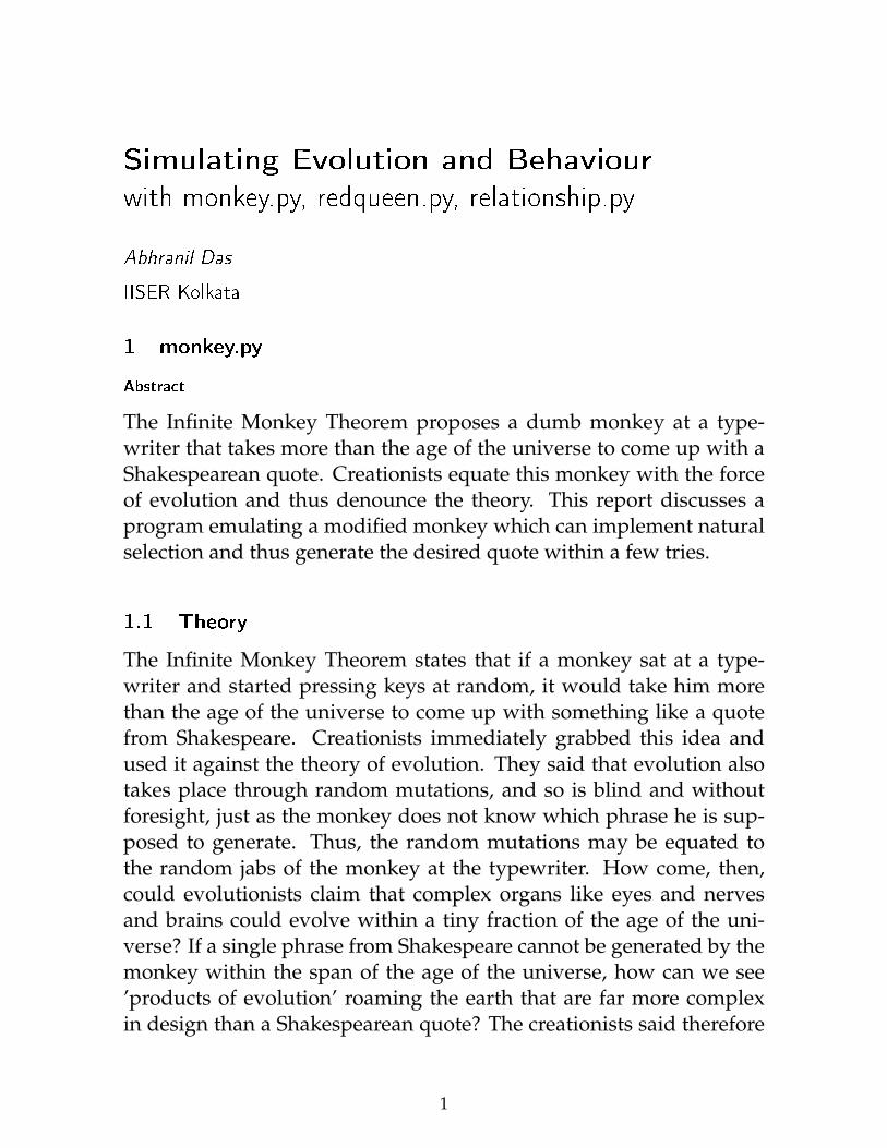
We can see how the phrase converges to the destination phrase, andthe fitness goes to 1. The following is the fitness v/s generation curve:

1 monkey.py 7
It is noticeable that the fitness curve goes asymptotically to 1. Thereason is that the fitter the phrase becomes, i.e. the closer it gets to thetarget phrase, the smaller is its chance of mutating again. So when itis very close to the target phrase, it requires a longer time to make achange.
This is, in fact, a point at which the analogy with evolution breaksdown. The asymptotic nature comes about because we fixed before-hand the target phrase. However, evolution is not teleological, in thatthere is no perfect organism towards which animals evolve. In a realfitness v/s generation plot, the trend will not be asymptotic.
Also notice that at some regions we have the fitness actually drop-ping. This is not surprising. It has an analog in real life: retrogradeevolution. I have zoomed in on a region of the plot that shows such athing.
1 monkey.py 8
This also shows up in the data file in generations 10 and 11:10 KmZXvy}p{tyv~td%_p-#$j^w))ojt\Zov~UzinvR- 0.807991696938
Km50vylp{tyv~td%_p-#$jnw)eojt\ZoL~Uzinv;- 0.787752983913
Cm@Xvy}p{tyv~td%_p-/8j^wf)ojt\Zo!~3ainvW- 0.758173326414
cm0X8y}p{tyv~t5%_p-#$"^w)yout\Zov~Uz(nvR- 0.785158277115
KN,Xvy}p{tyv~td%_p-#$j^wp>ojt\Zo9~qzinvR- 0.779968863518
Pm7Xvy_p{tyv~td%_p-#$j^w)/ojt\ZovuU7i\vR- 0.799688635184
11 Pm7Xvy_p{tyv~td%_p-#$j^w)/ojt\ZovuU7i\vR- 0.799688635184
We see that the fitness in generation 10 was 0.8, whereas that in 11came down to 0.79. If one has understood the working principle of theprogram, they shall see that such a thing is not impossible.
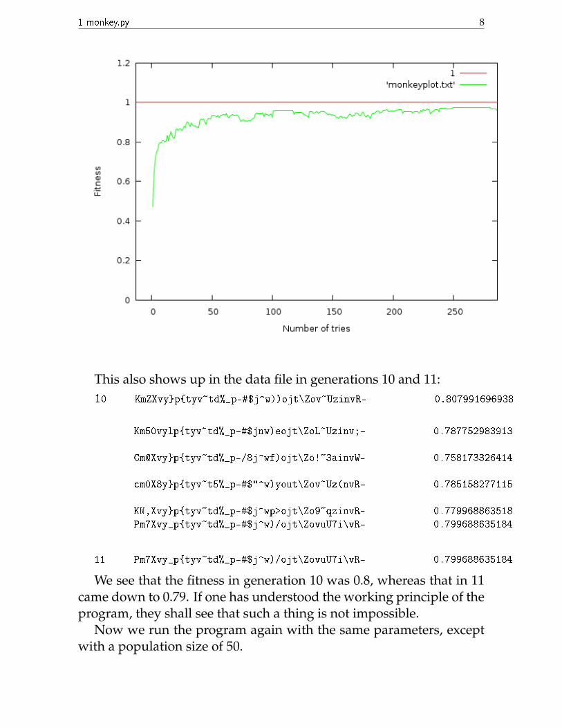
Now we run the program again with the same parameters, exceptwith a population size of 50.
1 monkey.py 9
The destination phrase is achieved in 743 tries. Then we try thesame thing with a population of 500:

1 monkey.py 10
The destination phrase arrives in 82 tries.We see that with increasing population size, the target phrase is
achieved quicker, and there is less retrograde evolution. Both of theseare easily understood. With a greater population size, there is a greaterchance of getting a mutated daughter that is closer to the target phrase.Thus, we reach the target quicker. And since the progeny is more innumber, it’s less probable that all of them will be less fit than the par-ent. Thus the chances of retrograde evolution are reduced.
1.5 Conclusions
i.) Thus, if the monkey is not all that dumb, but applies naturalselection, it can arrive at desired results pretty quickly.
ii.) Retrograde evolution can be observed. It reduces with largerpopulation size.
iv.) The number of tries requires for success drops with increas-ing population.
2 redqueen.py 11
ii.) Although teleology is a drawback of this simulation, withsome effort the concept of destination phrase that introducesthis teleology can be removed.
2 redqueen.py
Abstract
The Red Queen Hypothesis is associated with coevolution. This pro-gram simulates such co-evolution using two random variables depen-dent upon each other. The dependence of the coevolution pattern onvarious parameters is observed.
2.1 Theory
Coevolution occurs when two biologically evolving objects are relatedto each other. It may be as small as amino acids or as large as pheno-types of two species in an ecology. The Red Queen Hypothesis, origi-nally proposed by Leigh Van Valen (1973), is a model to describe thisevolutionary arms race.
In ’Through the Looking Glass’ by Lewis Carroll, the Red Queensays to Alice, ’It takes all the running you can do, to keep in the sameplace.’ In evolutionary biology, this quote can be translated to:
’An evolutionary system that co-evolves with other systems needsto continually develop to maintain its fitness relative to these othersystems.’
For example, the speed of a predator and that of its prey are coe-volving entities. Similarly, the colouration on a plant and a caterpillarthat camouflages on it are also coevolving. Another example is host-parasite interaction.
2.2 Aim
i.) To write a program for coevolution using a simplified model
ii.) To check whether coevolution occurs, and observing its na-ture
iii.) To see the effect of various parameters on the pattern of co-evolution
2 redqueen.py 12
2.3 The Program
The program was written in Python. It is the following:
1 # ! / usr / b in / python2 while True :3 l 1 = input ( ’ S t a r t value of s p e c i e s 1 : ’ )4 l 2 = input ( ’ S t a r t value of s p e c i e s 2 : ’ )5 pop1 = input ( ’ Population s i z e of s p e c i e s 1 : ’ )6 pop2 = input ( ’ Population s i z e of s p e c i e s 2 : ’ )7 N = input ( ’ Generation count : ’ )8 lpop1 = [ ’ ’ ]∗pop19 lpop2 = [ ’ ’ ]∗pop2
10 fpop1 = lpop1 [ : ]11 fpop2 = lpop2 [ : ]12 n = 113 import random , math , Gnuplot , commands14 def f i t n e s s ( i , u ) :15 return math . e∗∗(−abs ( i−u ) )16 f = open ( ’ redqueenplot . t x t ’ , ’w’ )17 g = open ( ’ redqueendata . t x t ’ , ’w’ )18 h = open ( ’ f i t n e s s p l o t . t x t ’ , ’w’ )19 print >> g , ’ S t a r t value of s p e c i e s 1 : ’ , l1 , ’\ t ’ , ’ S t a r t value of
s p e c i e s 2 : ’ , l 220 print >> g , ’ Population s i z e of s p e c i e s 1 : ’ , pop1 , ’\ t ’ , ’
Population s i z e of s p e c i e s 2 : ’ , pop221 print >> g , ’ Generation count : ’ , N22 print >> g , ’ Generation : ’ , ’\ t ’ , ’ Spec ies ’ , ’\ t ’ , ’ Value ’ , ’\ t ’ ∗2 ,
’ F i t n e s s ’23 while n <= N:24 print >> f , n , ’\ t ’ , l1 , ’\ t ’ , l 225 f i t = f i t n e s s ( l1 , l 2 )26 print >> g , n , ’\ t ’ ∗2 , ’ 1 ’ , ’\ t ’ , ’%17f ’%l1 , ’\ t ’ , ’%17f ’%(
f i t ) , ’\n ’27 for i in range ( pop1 ) :28 lpop1 [ i ] = l 129 #random m u t a t i o n s30 lpop1 [ i ] = random . normalvariate ( l1 , 1 0 )31 # f i t n e s s32 fpop1 [ i ] = f i t n e s s ( lpop1 [ i ] , l 2 )33 print >>g , ’\ t ’ ∗3 , ’%17f ’%lpop1 [ i ] , ’\ t ’ , fpop1 [ i ]34 print >> g , ’\n ’35 print >> g , ’\ t ’ ∗2 , ’ 2 ’ , ’\ t ’ , ’%17f ’%l2 , ’\ t ’ , ’%17f ’%( f i t
) , ’\n ’36 for i in range ( pop2 ) :37 lpop2 [ i ] = l 238 #random m u t a t i o n s39 lpop2 [ i ] = random . normalvariate ( l2 , 1 0 )40 # f i t n e s s41 fpop2 [ i ] = f i t n e s s ( lpop2 [ i ] , l 1 )42 print >> g , ’\ t ’ ∗3 , ’%17f ’%lpop2 [ i ] , ’\ t ’ , fpop2 [ i
]43 print >> g , ’\n ’44 print >> h , n , ’\ t ’ , f i t45 # n a t u r a l s e l e c t i o n46 def f i t t e s t ( l , lpop ) :

2 redqueen.py 13
47 lpoptemp = lpop [ : ]48 f = max( lpoptemp )49 while f > l :50 lpoptemp . remove (max( lpoptemp ) )51 i f len ( lpoptemp ) <> 0 :52 i f max( lpoptemp ) <= l :53 break54 e lse :55 break56 f = max( lpoptemp )57 return f58 l1 , l 2 = f i t t e s t ( l2 , lpop1 ) , f i t t e s t ( l1 , lpop2 )59 n += 160 f . c l o s e ( )61 g . c l o s e ( )62 h . c l o s e ( )63 commands . getoutput ( ’ ’ ’ gedi t ’ redqueendata . t x t ’ ’ ’ ’ )64 i = Gnuplot . Gnuplot ( )65 i ( ’ ’ ’ s e t t i t l e ’Red Queen Hypothesis : Phenotype Values with
Generation ’ ’ ’ ’ )66 i ( ’ ’ ’ s e t x l a b e l ’ Generation ’ ’ ’ ’ )67 i ( ’ ’ ’ s e t y l a b e l ’ Phenotype Values ’ ’ ’ ’ )68 i ( ’ ’ ’p ’ redqueenplot . t x t ’ u 1 : 2 w l t i t l e ’ Spec ies 1 ’ , ’
redqueenplot . t x t ’ u 1 : 3 w l t i t l e ’ Spec ies 2 ’ ’ ’ ’ )69 raw_input ( )70 i ( ’ ’ ’ s e t t i t l e ’Red Queen Hypothesis : F i t n e s s with Generation ’ ’
’ ’ )71 i ( ’ ’ ’ s e t x l a b e l ’ Generation ’ ’ ’ ’ )72 i ( ’ ’ ’ s e t y l a b e l ’ F i t n e s s ’ ’ ’ ’ )73 i ( ’ ’ ’p [ : ] [ 0 : 1 ] ’ f i t n e s s p l o t . t x t ’ w l t i t l e ’ F i t n e s s ’ ’ ’ ’ )
What does this program do? Well, what it does is that it takes twovariables, which can take number values. Each of the variables pro-duces mutated copies of themselves in one generation. These copieshave values that are generally different from the parent value fromwhich they are spawned. These mutated numbers are chosen througha gaussian distribution centered around the parent number and witha standard deviation of 10 units. One each of these mutated copiesare then chosen according to a fitness criterion. Up to this point it issimilar to monkey.py. But it is the fitness criterion that produces thecoevolution. Let’s say that my two variables are X and Y. The fitnesscriterion for X is that its value must be greater than that of Y, and thatof Y is that its value must be greater than the value of X.
Think of the two variables as signifying the phenotypes of two closelydependent species, let’s say the running speeds of a predator and itsprey. The predator hunts its prey by running it down. So it’s easilyseen that prey individuals who run faster than the predator survive.Similarly, predator individuals that run faster than their prey also sur-

2 redqueen.py 14
vive.One might think from this criterion that the fitness criteria have no
upper bound, meaning that any value that is greater than the currentvalue of the other variable is fit. Moreover, one might be tempted tothink that the larger the value, the greater the fitness. However, this iswrong. To see why, we need to go back to our example.
Let’s say that the average speed of the prey in one generation is 10m/s. Now, obviously, a particular predator individual benefits fromhaving a running speed greater than 10 m/s, but the higher its speedis, the more resources it is spending behind running. It is able to huntdown prey if it is faster than 10 m/s. It is not really necessary for itto run 50 m/s or 100 m/s. These are as good as 13 m/s. In fact, thepredator is worse off with these higher speeds because it costs its en-ergy resources. Therefore, the fittest value is the lowest speed that isgreater than the prey speed. This argument may be used in any otherscenario of coevolution, not just in cases of speed. Making a forwardmove in terms of evolution is costly, so only the smallest move neces-sary will be made, so that the gain reaped is highest for the smallestcost.
Therefore, our program first takes the values of the two variablesin generation i, say xi and yi. Then it generates two sets of mutatedvalues from these two. From the first set, it selects the value that isjust greater than yi. From the second set, it selects the value that is justgreater than xi. These two values then become xi+1 and yi+1.
The program takes five inputs: the starting values of the two species,the population sizes of the two species (this is the number of mutatedprogeny produced), and the number of generations to simulate. It pro-duces three outputs: a data file with all relevant information, a simul-taneous plot of the two values of the two species against generationnumber, and a plot of the fitness against generation.
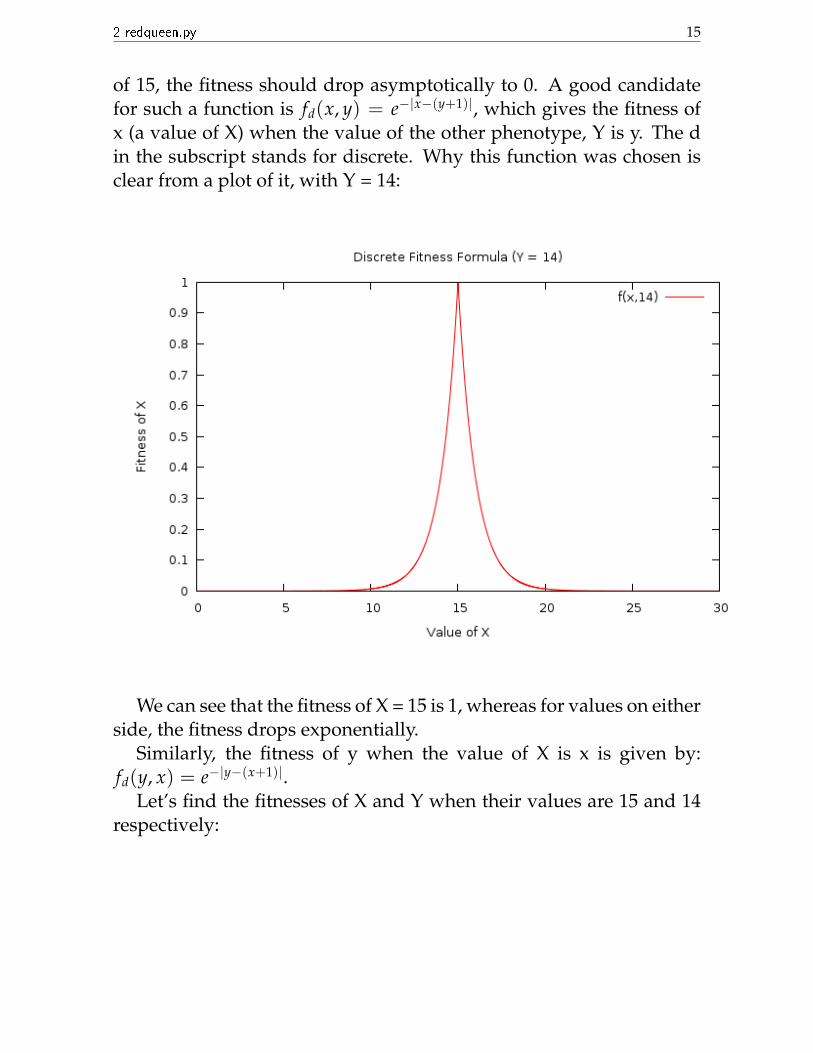
But there’s a catch here. We have defined what fittest is. But what isthe fitness value in general? We see that we don’t really need a numberassociated with fitness if we are anyway able to select the fittest. Butwe need a fitness against generation plot. For this reason alone weartificially define a fitness. To understand how we define it, we firstneed to assume that the values of the two variables are integral. Let’ssay that in one generation the value of Y is 14. Now, the fittest value ofX possible is 15, (with a fitness of 1), and as we go towards either side
2 redqueen.py 15
of 15, the fitness should drop asymptotically to 0. A good candidatefor such a function is fd(x, y) = e−|x−(y+1)|, which gives the fitness ofx (a value of X) when the value of the other phenotype, Y is y. The din the subscript stands for discrete. Why this function was chosen isclear from a plot of it, with Y = 14:
We can see that the fitness of X = 15 is 1, whereas for values on eitherside, the fitness drops exponentially.
Similarly, the fitness of y when the value of X is x is given by:fd(y, x) = e−|y−(x+1)|.
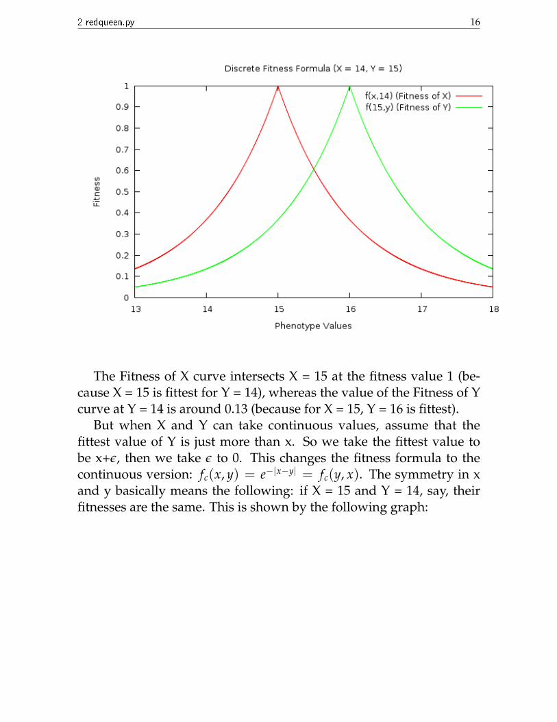
Let’s find the fitnesses of X and Y when their values are 15 and 14respectively:
2 redqueen.py 16
The Fitness of X curve intersects X = 15 at the fitness value 1 (be-cause X = 15 is fittest for Y = 14), whereas the value of the Fitness of Ycurve at Y = 14 is around 0.13 (because for X = 15, Y = 16 is fittest).
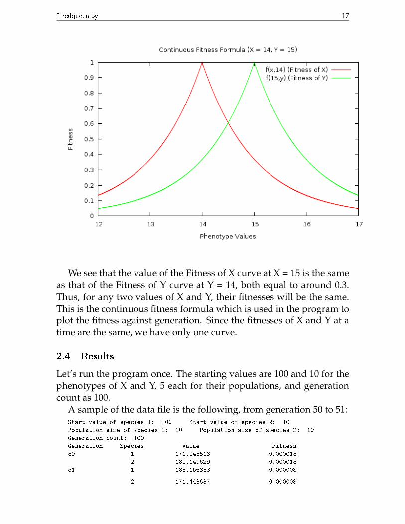
But when X and Y can take continuous values, assume that thefittest value of Y is just more than x. So we take the fittest value tobe x+ε, then we take ε to 0. This changes the fitness formula to thecontinuous version: fc(x, y) = e−|x−y| = fc(y, x). The symmetry in xand y basically means the following: if X = 15 and Y = 14, say, theirfitnesses are the same. This is shown by the following graph:
2 redqueen.py 17
We see that the value of the Fitness of X curve at X = 15 is the sameas that of the Fitness of Y curve at Y = 14, both equal to around 0.3.Thus, for any two values of X and Y, their fitnesses will be the same.This is the continuous fitness formula which is used in the program toplot the fitness against generation. Since the fitnesses of X and Y at atime are the same, we have only one curve.
2.4 Results
Let’s run the program once. The starting values are 100 and 10 for thephenotypes of X and Y, 5 each for their populations, and generationcount as 100.
A sample of the data file is the following, from generation 50 to 51:Start value of species 1: 100 Start value of species 2: 10
Population size of species 1: 10 Population size of species 2: 10
Generation count: 100
Generation Species Value Fitness
50 1 171.045513 0.000015
2 182.149629 0.000015
51 1 183.156338 0.000008
2 171.443637 0.000008
2 redqueen.py 18
We can see that the values 171.04 and 182.14 become 183.15 and171.44, which is almost a flip with an upward shift.
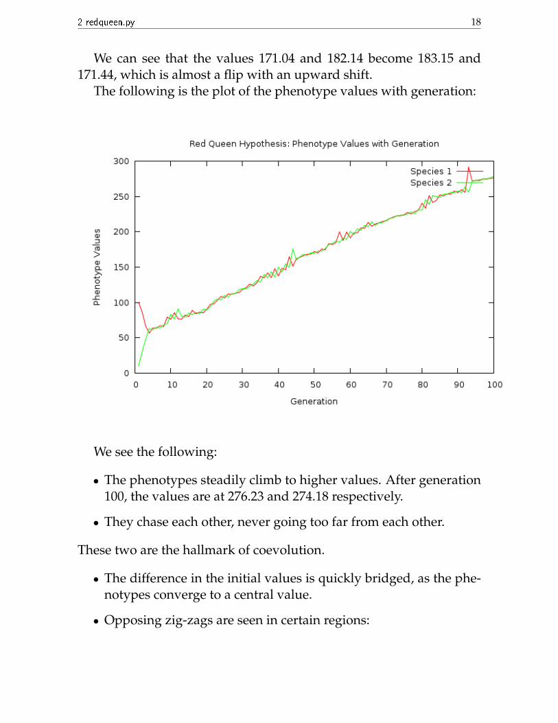
The following is the plot of the phenotype values with generation:
We see the following:
• The phenotypes steadily climb to higher values. After generation100, the values are at 276.23 and 274.18 respectively.
• They chase each other, never going too far from each other.
These two are the hallmark of coevolution.
• The difference in the initial values is quickly bridged, as the phe-notypes converge to a central value.
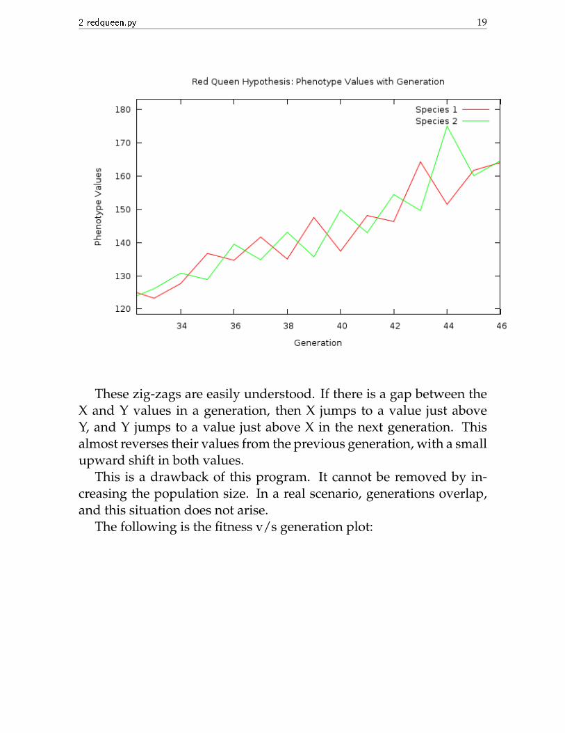
• Opposing zig-zags are seen in certain regions:
2 redqueen.py 19
These zig-zags are easily understood. If there is a gap between theX and Y values in a generation, then X jumps to a value just aboveY, and Y jumps to a value just above X in the next generation. Thisalmost reverses their values from the previous generation, with a smallupward shift in both values.
This is a drawback of this program. It cannot be removed by in-creasing the population size. In a real scenario, generations overlap,and this situation does not arise.
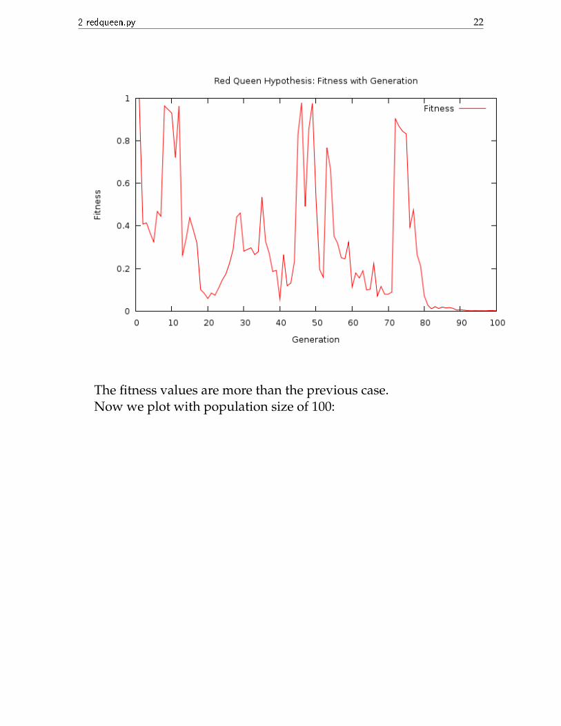
The following is the fitness v/s generation plot:

2 redqueen.py 20
We see that the fitness value is not really increasing on the aver-age over time, although the species are continually evolving. This isthe crux of the Red Queen Hypothesis. There is a need for continualevolution just to maintain the fitness.
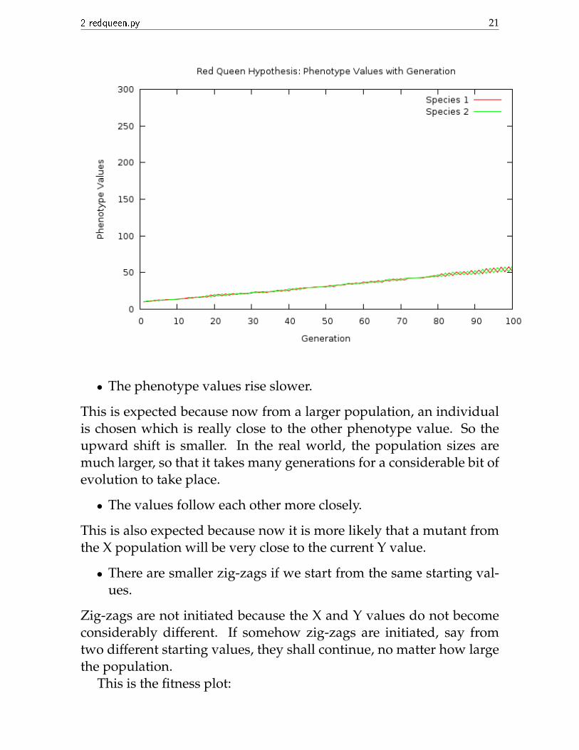
Now we run the program again. This time we take both initial val-ues to be 10, in order to minimize zig-zags, and a larger populationsize of 50. We plot the phenotype values in the same y range as theprevious plot in order to compare:
2 redqueen.py 21
• The phenotype values rise slower.
This is expected because now from a larger population, an individualis chosen which is really close to the other phenotype value. So theupward shift is smaller. In the real world, the population sizes aremuch larger, so that it takes many generations for a considerable bit ofevolution to take place.
• The values follow each other more closely.
This is also expected because now it is more likely that a mutant fromthe X population will be very close to the current Y value.
• There are smaller zig-zags if we start from the same starting val-ues.
Zig-zags are not initiated because the X and Y values do not becomeconsiderably different. If somehow zig-zags are initiated, say fromtwo different starting values, they shall continue, no matter how largethe population.
This is the fitness plot:
2 redqueen.py 22
The fitness values are more than the previous case.Now we plot with population size of 100:

2 redqueen.py 23
2 redqueen.py 24
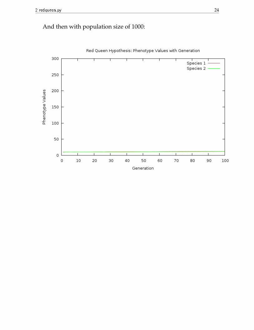
And then with population size of 1000:

2 redqueen.py 25
We can see that the increase of phenotype values with generation isvery slow, but it is not zero.
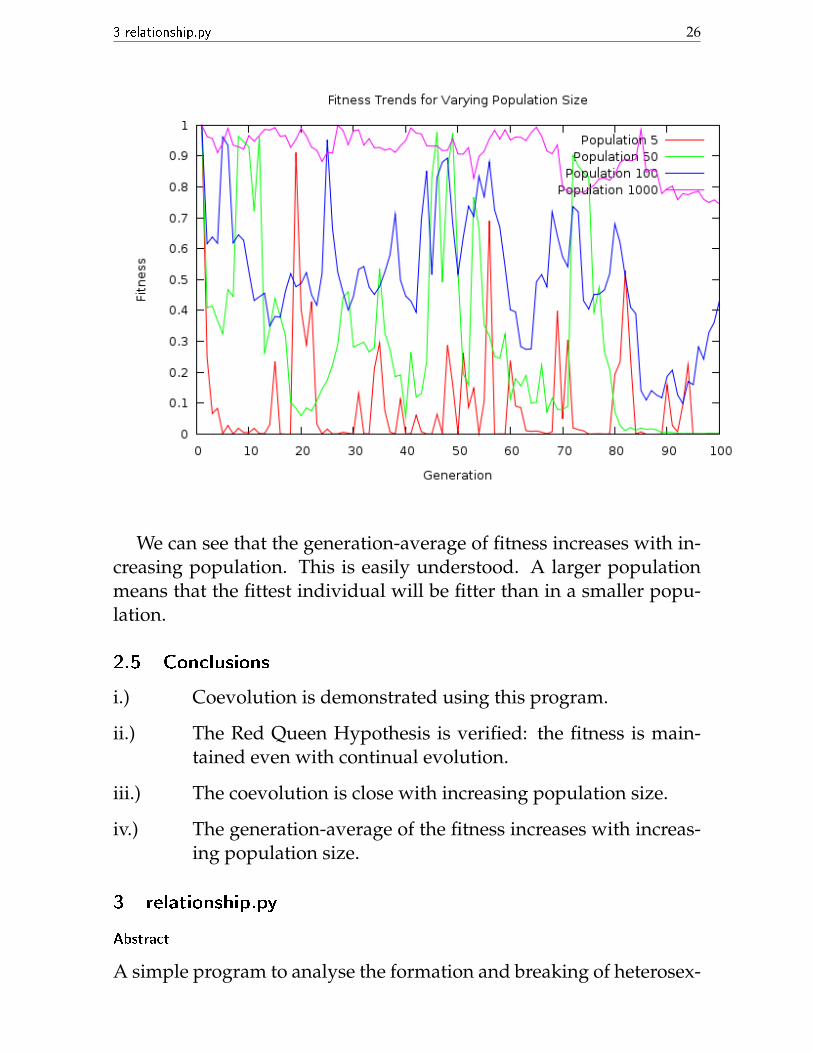
Here is a plot of the fitness against generation for the different pop-ulation sizes:
3 relationship.py 26
We can see that the generation-average of fitness increases with in-creasing population. This is easily understood. A larger populationmeans that the fittest individual will be fitter than in a smaller popu-lation.
2.5 Conclusions
i.) Coevolution is demonstrated using this program.
ii.) The Red Queen Hypothesis is verified: the fitness is main-tained even with continual evolution.
iii.) The coevolution is close with increasing population size.
iv.) The generation-average of the fitness increases with increas-ing population size.
3 relationship.py
Abstract
A simple program to analyse the formation and breaking of heterosex-

3 relationship.py 27
ual relationships in a population of singles and couples, and the effectof the values of various parameters on the result.
3.1 Theory
The theory involved with this program is very simple. We know thata heterosexual human population consists of single males, single fe-males and couples. These elements may be supposed to roam freelythrough their world, often chancing upon enocunters. There may bedifferent types of encounters: a single male with another single male,a single female with another single female, a single male with a singlefemale, and encounters between committed persons. When a singlemale meets (read encounters, interacts, and familiarizes with) a singlefemale, there is a certain chance that they shall commit themselves toa relationship. For purposes of simplification, we assume that othersorts of encounters do not amount to the formation of any relation-ship. In particular, it may be assumed that couples are isolated fromthe rest of the world, in that they have already committed themselvesto a relationship, and in the duration of it, will not be involved in anyencounters that break or form a relationship. This is surely a draw-back of the program, because in many cases committed persons aretempted by single persons, which results in the breaking and makingof relationships. But here we neglect that.
Once in a relationship, there is the chance of a break-up. If thishappens, the persons forming that couple are released into the world,when they can again chance upon encounters.
3.2 Aim
i.) To write a program to simulate a population of heterosexualsmaking and breaking relationships
ii.) To observe the results for different initial settings
iii.) To attempt to get a balanced condition where the number ofcommitted persons equals the number of single persons.
3.3 The Program
The program was written in Python. It is the following:

3 relationship.py 28
1 # ! /usr/bin/python2 while True :3 f = input ( ’ Number of s i n g l e females : ’ )4 m = input ( ’ Number of s i n g l e males : ’ )5 c = input ( ’ Number of couples : ’ )6 pc = input ( ’ P r o b a b i l i t y of commitment : ’ )7 pb = input ( ’ P r o b a b i l i t y of break−up : ’ )8 import random , Gnuplot9 h = Gnuplot . Gnuplot ( )
10 h ( ’ ’ ’ s e t t i t l e ’ R e l a t i o n s h i p s : M %d F %d C %d PC %fPB %f ’ ’ ’ ’%(m, f , c , pc , pb ) )
11 g = open ( ’ r e l a t i o n s h i p . t x t ’ , ’w’ )12 pr int >> g , 1 , ’\ t ’ , m , ’\ t ’ , f , ’\ t ’ , c13 f o r i in range ( ( f +m) ∗ ( f +m−1)/2) :14 i f f ∗m > 0 :15 x = random . sample ( range ( f +m) , 2 )16 i f ( x [0]− ( f − 0 . 5 ) ) ∗ ( x [1]− ( f − 0 . 5 ) ) < 0 :17 i f random . uniform ( 0 , 1 ) <= pc :18 f −= 119 m −= 120 c += 121 i f c > 0 :22 i f random . uniform ( 0 , 1 ) <=pb :23 f += 124 m += 125 c −= 126 print >> g , i +1 , ’\ t ’ , m , ’\ t ’ , f , ’\ t ’ , c27 g . c l o s e ( )28 h ( ’ ’ ’ s e t x l a b e l ’ I t e r a t i o n s ’ ’ ’ ’ )29 h ( ’ ’ ’ s e t y l a b e l ’Number ’ ’ ’ ’ )30 h ( ’ ’ ’ p ’ r e l a t i o n s h i p . t x t ’ u 1 : 2 w l t i t l e ’ Males ’ , ’ r e l a t i o n s h i p
. t x t ’ u 1 : 3 w l t i t l e ’ Females ’ , ’ r e l a t i o n s h i p . t x t ’ u 1 : 4 w lt i t l e ’ Couples ’ ’ ’ ’ )
What the program does is the following: it takes the starting num-ber of single females, single males and couples, and the probabilities ofcommitment and break-up. Then it starts taking random samples (SR-SWOR) of size two from the population of the singles. If a male and afemale come up, they may get committed with the preset probabilityvalue. If they are committed, they are removed from the population.Simultaneously, the couples are broken up with the preset probabilityvalue, upon which they enter the population again. The number oftimes this operation is done is equal to the total number of possiblecollisions. This is because when the population size is larger, there arealso more collisions per unit time. So, if we are to see the time evolu-tion of the system, each time step should contain more collisions if thepopulation size is more. Thus, if instead of defining a time step thatcontains more iterations for a greater population, we might just takethe total number of collisions as the range of iterations over which to

3 relationship.py 29
plot the graph. This way, we can say that all the graphs generated takeplace more or less in the same duration.
The principle is somewhat like Brownian motion. The single per-sons may be assumed to execute this random motion, and sometimesthere is a collision between a male and a female. If they enter into a re-lationship, they are precipitated from the system. The precipitate at thebottom, consisting in couples, also releases molecules into the systemwith a finite chance. A dynamic equilibrium may thus be establishedbetween committed and single persons.
The program then plots the number of single males, single femalesand couples against iteration number, using gnuplot.
3.4 Results
This is a sample plot for number of single females (F) = 50, numberof single males (M) = 100, number of couples (C) = 50, probability ofcommitment (PC) = 0 and probability of break-up (PB) = 1:

3 relationship.py 30
We see that starting from the initial values, the scenario changessteadily and monotonically to zero couples, and all persons single.
Now we keep the population same, but change PC to 0.3, and PB to0.7:
The situation is more or less the same, but now there are some fluc-tuations from the steady state, which are quickly restored.
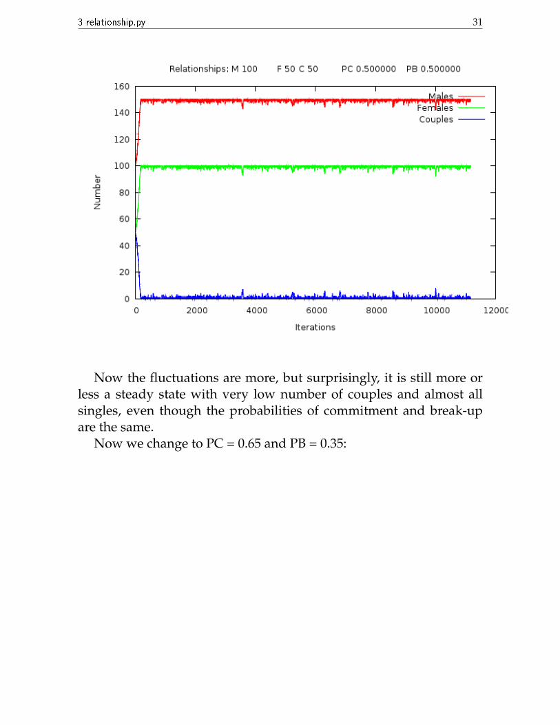
Now we change to PC = 0.5, PB = 0.5:
3 relationship.py 31
Now the fluctuations are more, but surprisingly, it is still more orless a steady state with very low number of couples and almost allsingles, even though the probabilities of commitment and break-upare the same.
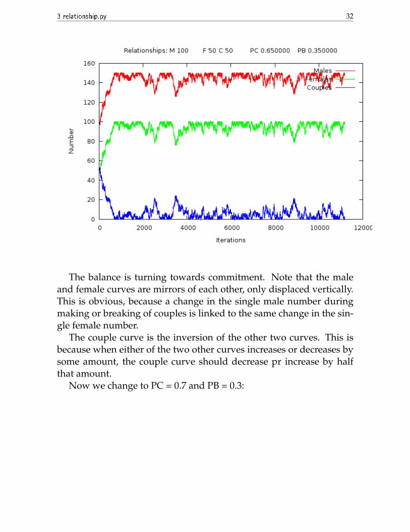
Now we change to PC = 0.65 and PB = 0.35:
3 relationship.py 32
The balance is turning towards commitment. Note that the maleand female curves are mirrors of each other, only displaced vertically.This is obvious, because a change in the single male number duringmaking or breaking of couples is linked to the same change in the sin-gle female number.
The couple curve is the inversion of the other two curves. This isbecause when either of the two other curves increases or decreases bysome amount, the couple curve should decrease pr increase by halfthat amount.
Now we change to PC = 0.7 and PB = 0.3:

3 relationship.py 33
This cannot really be called a steady state. Moreover, now the bal-ance is in equal favour of single and committed people. The couplecurve is more or less midway between the single curves, which meansthat double of the couple curve (the number of committed people) isthe sum of the single males and single females (total number of singlepeople).
Now we change to PC = 0.9, PB = 0.1:

3 relationship.py 34
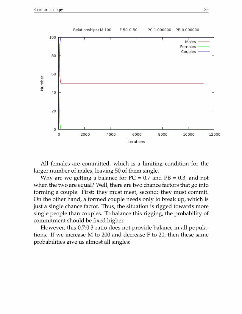
The balance is now turning towards couples.And finally, for PC = 1 and PB = 0:
3 relationship.py 35
All females are committed, which is a limiting condition for thelarger number of males, leaving 50 of them single.
Why are we getting a balance for PC = 0.7 and PB = 0.3, and notwhen the two are equal? Well, there are two chance factors that go intoforming a couple. First: they must meet, second: they must commit.On the other hand, a formed couple needs only to break up, which isjust a single chance factor. Thus, the situation is rigged towards moresingle people than couples. To balance this rigging, the probability ofcommitment should be fixed higher.
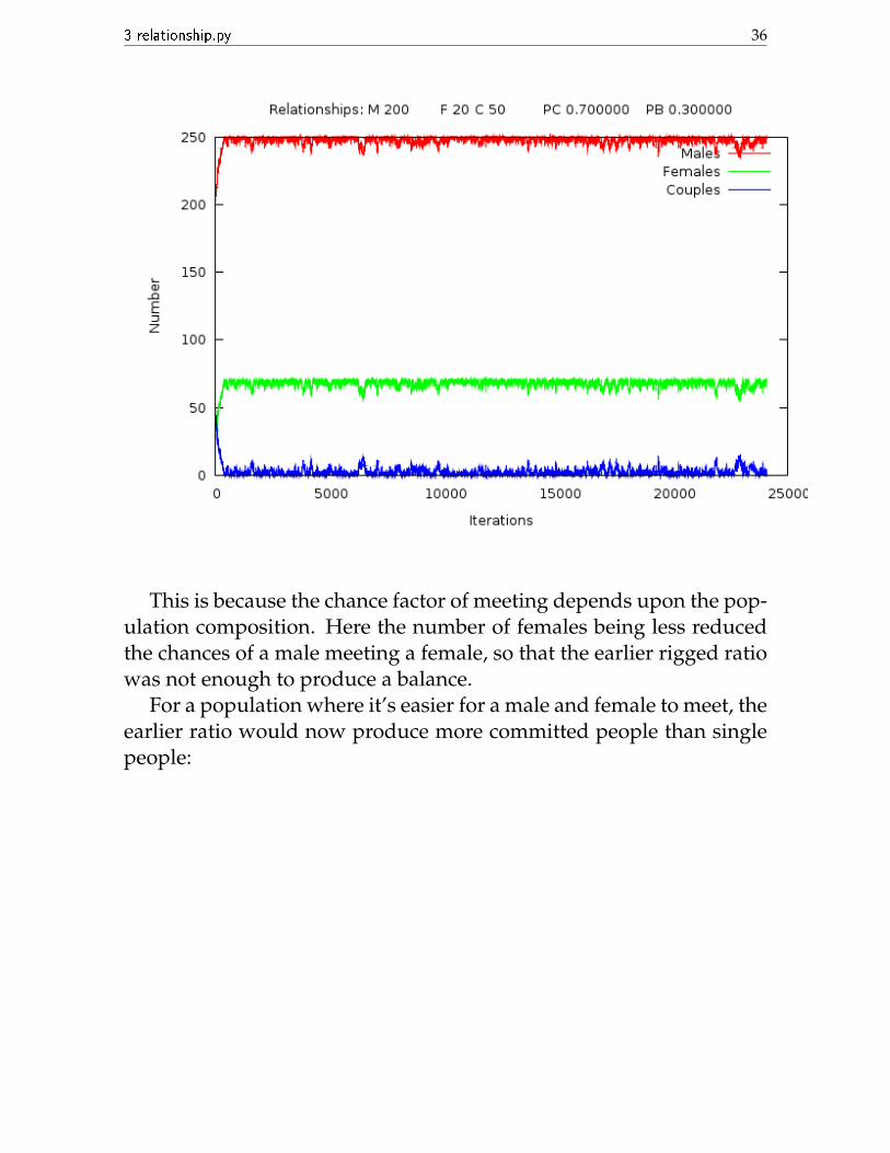
However, this 0.7:0.3 ratio does not provide balance in all popula-tions. If we increase M to 200 and decrease F to 20, then these sameprobabilities give us almost all singles:
3 relationship.py 36
This is because the chance factor of meeting depends upon the pop-ulation composition. Here the number of females being less reducedthe chances of a male meeting a female, so that the earlier rigged ratiowas not enough to produce a balance.
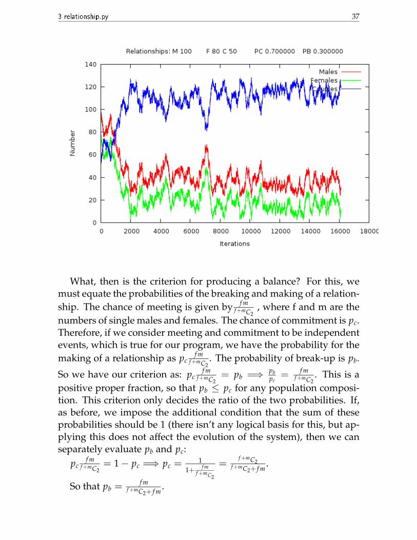
For a population where it’s easier for a male and female to meet, theearlier ratio would now produce more committed people than singlepeople:
3 relationship.py 37
What, then is the criterion for producing a balance? For this, wemust equate the probabilities of the breaking and making of a relation-ship. The chance of meeting is given by f m
f +mC2, where f and m are the
numbers of single males and females. The chance of commitment is pc.Therefore, if we consider meeting and commitment to be independentevents, which is true for our program, we have the probability for themaking of a relationship as pc
f mf +mC2
. The probability of break-up is pb.
So we have our criterion as: pcf m
f +mC2= pb =⇒ pb
pc= f m
f +mC2. This is a
positive proper fraction, so that pb ≤ pc for any population composi-tion. This criterion only decides the ratio of the two probabilities. If,as before, we impose the additional condition that the sum of theseprobabilities should be 1 (there isn’t any logical basis for this, but ap-plying this does not affect the evolution of the system), then we canseparately evaluate pb and pc:
pcf m
f +mC2= 1− pc =⇒ pc = 1
1+ f mf +mC2
=f +mC2
f +mC2+ f m.
So that pb = f mf +mC2+ f m
.

3 relationship.py 38
We see that the balance condition probabilities do not depend onthe number of couples.
For f = 50 and m = 100, our first example, we have pc = 0.69 ,pb = 0.31. This is very close to our empirical values of 0.7 and 0.3.
For the second example, (m=200, f=20, c=50), we have pc = 0.85 ,pb = 0.15. The following plot shows this:
Now we are in for a surprise. The couple curve is not midway be-tween the other two curves, so that the system is not balanced. Whydid this happen? Well, close observation shows that with this initialpopulation composition, it is impossible to equate the number of com-mitted and single people. If we try to raise the couple curve, we haveto lower the other two curves by the same distance, but the femalecurve will touch the baseline.
There is a criterion on the initial values for the system to be able toreach a balance.
Let’s take our initial values to be f, m, and c. Let’s say x females (ormales) need to get committed from the initial value to reach a balance.
3 relationship.py 39
x may be positive or negative (meaning couples need to break to jointhe single population). So in the balance condition we have:
f − x + m− x = 2(c + x) =⇒ x = f +m−2c4 .
Now, the upper limit of x is the number of single females if theyare fewer than males, because once all females are committed, therecannot be any more commitments. Similarly, if males are fewer thanfemales, the upper limit of x is the number of males.
The lower limit of x is simply -c, because that many males (or fe-males) from the couple population can join in the single male (or fe-male) population.
∴ x ε [−c, min{ f , m}]=⇒ −c ≤ f +m−2c
4 ≤min{ f , m}The lower limit can be written as:−4c ≤ f + m − 2c =⇒ −2c ≤ f + m, which is always true since
f + m is positive. So we may ignore the lower limit.Therefore, the condition on the initial values for the system to allow
a balance is: f + m− 2c ≤ 4min{ f , m}.So even though the balance condition does not depend on the num-
ber of couples, the balance criterion depends on it. For a wrong valueof c, we can never have balance.
In the last case that we considered, we have the L.H.S. = 200 + 20−2× 50 = 120. The R.H.S. = 4× 20 = 80. ∵ 120 � 80, we could notreach a balance even with optimum probability values.
Now let’s consider our first example, with f = 50, m = 100, c = 50.We have the L.H.S. = 50 + 100− 100 = 50. The R.H.S. = 4× 50 = 200.So the balance threshold was satisfied, and we got a balance.
For the third example (f = 80, m = 100, c = 50), we have 80 ≤ 120, soa balance can be achieved.
The balance condition is given by pc = 0.668187474,pb = 0.331812525.If you are wondering why I have put so many decimal places, it willbe clear shortly. First let us plot the balanced state:

3 relationship.py 40
The end bit does not look very balanced, so it’s difficult to believethat this is the balanced condition. However, to convince you, I shalltake slightly different values of the probabilities.
Let’s take pc = 0.68,pb = 0.32:
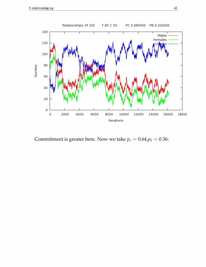
3 relationship.py 41
Commitment is greater here. Now we take pc = 0.64,pb = 0.36:

3 relationship.py 42
Almost all are single. So we see that the change of 2 in the secondplace of decimal of the probabilities causes such a drastic change. Thatis why I had to be so accurate in the balance condition probabilities.
A look at the graphs also tells us another important thing: the bal-ance condition is an unstable equilibrium. This is why, even withthe balance condition probabilities, the system tends to deviate frombalance, whereas with slightly different probabilities, it stabilizes faraway from the balance.
3.5 Conclusions
i.) The relationship model is successfully simulated
ii.) For a balance condition, the probability of commitment needsto be more than the probability of break-up.
iii.) There is a balance threshold dependent on the populationcomposition which has to be satisfied for a balance to be al-lowed.
3 relationship.py 43
iv.) If the balance threshold is satisfied, there is a balance condi-tion depending upon the population composition which willgive us a balance.
v.) The balance condition is an unstable equilibrium.
Acknowledgements
• The Python programming language
• LYX document processor (LATEX)
• Dr. Anindita Bhadra