Simulated Annealing

Iterative Improvement 1Iterative Improvement 1• General method to solve combinatorial

optimization problems

Principle:• Start with initial configuration• Repeatedly search neighborhood and select a

neighbor as candidate• Evaluate some cost function (or fitness function)

and accept candidate if "better"; if not, select another neighbor

• Stop if quality is sufficiently high, if no improvement can be found or after some fixed time

Iterative Improvement 2

Needed are:• A method to generate initial configuration• A transition or generation function to find a

neighbor as next candidate• A cost function• An Evaluation Criterion• A Stop Criterion

Iterative Improvement 3

Simple Iterative Improvement or Hill Climbing:• Candidate is always and only accepted if cost is

lower (or fitness is higher) than current configuration

• Stop when no neighbor with lower cost (higher fitness) can be found

Disadvantages:• Local optimum as best result• Local optimum depends on initial configuration• Generally no upper bound on iteration length

Hill climbingHill climbing

Convergence of Convergence of simulated annealing simulated annealing

HILL CLIMBING

HILL CLIMBING

HILL CLIMBINGCO

ST

FU

NC

TIO

N, C

NUMBER OF ITERATIONS

AT INIT_TEMP

AT FINAL_TEMP

Move accepted withprobability= e-(^C/temp)

Unconditional Acceptance

How to cope with disadvantages

• Repeat algorithm many times with different initial configurations

• Use information gathered in previous runs• Use a more complex Generation Function to jump

out of local optimum• Use a more complex Evaluation Criterion that

accepts sometimes (randomly) also solutions away from the (local) optimum

Simulated AnnealingSimulated Annealing

Use a more complex Evaluation Function:• Do sometimes accept candidates with higher cost

to escape from local optimum• Adapt the parameters of this Evaluation Function

during execution• Based upon the analogy with the simulation of

the annealing of solids

Other Names

• Monte Carlo Annealing• Statistical Cooling• Probabilistic Hill Climbing• Stochastic Relaxation• Probabilistic Exchange Algorithm

Analogy

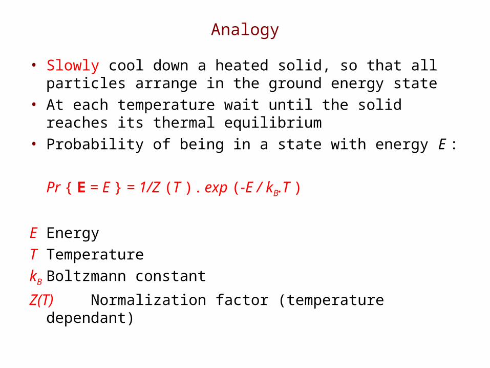
• Slowly cool down a heated solid, so that all particles arrange in the ground energy state

• At each temperature wait until the solid reaches its thermal equilibrium

• Probability of being in a state with energy E :

Pr { E = E } = 1/Z (T ) . exp (-E / kB.T )

E EnergyT TemperaturekB Boltzmann constant

Z(T) Normalization factor (temperature dependant)

Simulation of cooling (Metropolis 1953)

• At a fixed temperature T :• Perturb (randomly) the current state to a new state E is the difference in energy between current and

new state• If E < 0 (new state is lower), accept new state as

current state• If E 0 , accept new state with probability

Pr (accepted) = exp (- E / kB.T)

• Eventually the systems evolves into thermal equilibrium at temperature T ; then the formula mentioned before holds

• When equilibrium is reached, temperature T can be lowered and the process can be repeated

Performance

• SA is a general solution method that is easily applicable to a large number of problems

• "Tuning" of the parameters (initial c, decrement of c, stop criterion) is relatively easy

• Generally the quality of the results of SA is good, although it can take a lot of time

• Results are generally not reproducible: another run can give a different result

• SA can leave an optimal solution and not find it again(so try to remember the best solution found so far)

• Proven to find the optimum under certain conditions; one of these conditions is that you must run forever

Theoretical Results

• If the temperature T is kept constant,• then the transition matrix,Pij , is independent of

the iteration number.• Correspond to a homogeneous Markov chain• The stationary distribution q(i) , corresponds to

Boltzmann distribution. • The limit as T→0 of this stationary distribution is a

uniform distribution over set of optimal solutions.• The SA algorithm converges to the set of globally

optimal solutions.• But this result does not tell us anything about the

number of iterations required to achieve convergence.

Algorithm• 1.      Select an objective function E(x);• 2.      Select an initial temperature T>0;• 3.      Set temperature change counter t=0;• 4.      Repeat• 4.1  Set repetition counter n=0;• 4.2  Repeat• 4.2.1   Generate state xi+1, a neighbor of xi;

• 4.2.2   Calculate E=E(xi+1)E(xi);

• 4.2.3   If E<0 then xi=xi+1;

• 4.2.4   else if random(0,1)<exp(E/T) then xi=xi+1;• 4.2.5   n=n+1;• 4.3  Until n=r(t);• 4.4  t=t+1;• 4.5  T=T(t);• Until stopping criterion true. 

Generic Choices

• Kirkpatrick et al. (1983)• Set initial value T to be large enough • T(t+1)= T(t), :0.8~0.99 • N(t): a sufficient number of transitions

corresponding to thermal equilibriumconstantor proportional to the size of the neighborhood

• Stopping criterionwhen the solution obtained at each temperature

change is unaltered for a number of consecutive temperature changes. (T…T/10)

SA Cooling Schedule

• Starting Temperature

• Final Temperature

• Temperature Decrement

• Iterations at each temperature

SA Cooling Schedule - Starting Temperature

• Starting Temperature

• Must be hot enough to allow moves to almost neighbourhood state (else we are in danger of implementing hill climbing)

• Must not be so hot that we conduct a random search for a period of time

• Problem is finding a suitable starting temperature

SA Cooling Schedule - Final Temperature

• Final Temperature - Choosing

• It is usual to let the temperature decrease until it reaches zero However, this can make the algorithm run for a lot longer.

• Therefore, the stopping criteria can either be a suitably low temperature or when the system is “frozen” at the current temperature (i.e. no better or worse moves are being accepted)

SA Cooling Schedule - Temperature Decrement

• Temperature Decrement

• Theory states that we should allow enough iterations at each temperature so that the system stabilises at that temperature

• Unfortunately, theory also states that the number of iterations at each temperature to achieve this might be exponential to the problem size

• Doing a large number of iterations at a few temperatures, a small number of iterations at many temperatures or a balance between the two

SA Cooling Schedule - Temperature Decrement

• Temperature Decrement

• Linear

temp = temp - x

• Geometric

temp = temp * xExperience has shown that α should be between 0.8 and 0.99, with better results being found in the higher end of the range. Of course, the higher the value of α, the longer it will take to decrement the temperature to the stopping criterion

SA Cooling Schedule - Iterations

• Iterations at each temperature

• A constant number of iterations at each temperature

• The formula used by Lundy ist = t/(1 + βt)

where β is a suitably small value

Conclusions

• It is very easy to implement.• It can be generally applied to a wide range

of problems.• SA can provide high quality solutions to

many problems.• Care is needed to devise an appropriate

neighborhood structure and cooling scheduler to obtain an efficient algorithm.