simplified system efficiency functions for linear phased-array … · 2017-05-03 · simplified...

Center for Nondestructive Evaluation ConferencePapers, Posters and Presentations Center for Nondestructive Evaluation

7-2009

Simplified system efficiency functions for linearphased-array transducersFrank J. MargetanIowa State University, [email protected]

Timothy A. GrayIowa State University, [email protected]

Ruiju Huang

Follow this and additional works at: http://lib.dr.iastate.edu/cnde_conf

Part of the Materials Science and Engineering Commons, and the Structures and MaterialsCommons

The complete bibliographic information for this item can be found at http://lib.dr.iastate.edu/cnde_conf/64. For information on how to cite this item, please visit http://lib.dr.iastate.edu/howtocite.html.

This Conference Proceeding is brought to you for free and open access by the Center for Nondestructive Evaluation at Digital Repository @ Iowa StateUniversity. It has been accepted for inclusion in Center for Nondestructive Evaluation Conference Papers, Posters and Presentations by an authorizedadministrator of Digital Repository @ Iowa State University. For more information, please contact [email protected].

http://lib.dr.iastate.edu/?utm_source=lib.dr.iastate.edu%2Fcnde_conf%2F64&utm_medium=PDF&utm_campaign=PDFCoverPages

http://lib.dr.iastate.edu/?utm_source=lib.dr.iastate.edu%2Fcnde_conf%2F64&utm_medium=PDF&utm_campaign=PDFCoverPages

http://lib.dr.iastate.edu/cnde_conf?utm_source=lib.dr.iastate.edu%2Fcnde_conf%2F64&utm_medium=PDF&utm_campaign=PDFCoverPages


http://lib.dr.iastate.edu/cnde?utm_source=lib.dr.iastate.edu%2Fcnde_conf%2F64&utm_medium=PDF&utm_campaign=PDFCoverPages


http://network.bepress.com/hgg/discipline/285?utm_source=lib.dr.iastate.edu%2Fcnde_conf%2F64&utm_medium=PDF&utm_campaign=PDFCoverPages



http://lib.dr.iastate.edu/cnde_conf/64

http://lib.dr.iastate.edu/cnde_conf/64

http://lib.dr.iastate.edu/howtocite.html

http://lib.dr.iastate.edu/howtocite.html

mailto:[email protected]

SIMPLIFIED SYSTEM EFFICIENCY FUNCTIONS FOR LINEAR PHASEDARRAY TRANSDUCERSF. J. Margetan, T. A. Gray, and Ruiju Huang Citation: AIP Conf. Proc. 1211, 879 (2010); doi: 10.1063/1.3362513 View online: http://dx.doi.org/10.1063/1.3362513 View Table of Contents: http://proceedings.aip.org/dbt/dbt.jsp?KEY=APCPCS&Volume=1211&Issue=1 Published by the American Institute of Physics. Related ArticlesResonance ultrasonic thermography: Highly efficient contact and air-coupled remote modes Appl. Phys. Lett. 102, 061905 (2013) Probing of laser-induced crack closure by pulsed laser-generated acoustic waves J. Appl. Phys. 113, 014906 (2013) Investigating and understanding fouling in a planar setup using ultrasonic methods Rev. Sci. Instrum. 83, 094904 (2012) A local defect resonance to enhance acoustic wave-defect interaction in ultrasonic nondestructive evaluation Appl. Phys. Lett. 99, 211911 (2011) Time reversed acoustics techniques for elastic imaging in reverberant and nonreverberant media: Anexperimental study of the chaotic cavity transducer concept J. Appl. Phys. 109, 104910 (2011) Additional information on AIP Conf. Proc.Journal Homepage: http://proceedings.aip.org/ Journal Information: http://proceedings.aip.org/about/about_the_proceedings Top downloads: http://proceedings.aip.org/dbt/most_downloaded.jsp?KEY=APCPCS Information for Authors: http://proceedings.aip.org/authors/information_for_authors

Downloaded 12 Feb 2013 to 129.186.176.91. Redistribution subject to AIP license or copyright; see http://proceedings.aip.org/about/rights_permissions

http://proceedings.aip.org/?ver=pdfcov

http://aipadvances.aip.org?ver=pdfcov

http://scitation.aip.org/vsearch/servlet/VerityServlet?KEY=ALL&uSeDeFaUlTkEy=TrUe&possible1=F. J. Margetan&possible1zone=author&maxdisp=25&smode=strresults&aqs=true&ver=pdfcov

http://scitation.aip.org/vsearch/servlet/VerityServlet?KEY=ALL&uSeDeFaUlTkEy=TrUe&possible1=T. A. Gray&possible1zone=author&maxdisp=25&smode=strresults&aqs=true&ver=pdfcov

http://scitation.aip.org/vsearch/servlet/VerityServlet?KEY=ALL&uSeDeFaUlTkEy=TrUe&possible1=Ruiju Huang&possible1zone=author&maxdisp=25&smode=strresults&aqs=true&ver=pdfcov


http://link.aip.org/link/doi/10.1063/1.3362513?ver=pdfcov

http://proceedings.aip.org/dbt/dbt.jsp?KEY=APCPCS&Volume=1211&Issue=1&ver=pdfcov

http://www.aip.org/?ver=pdfcov







http://proceedings.aip.org/about/about_the_proceedings?ver=pdfcov

http://proceedings.aip.org/dbt/most_downloaded.jsp?KEY=APCPCS&ver=pdfcov

http://proceedings.aip.org/authors/information_for_authors?ver=pdfcov

SIMPLIFIED SYSTEM EFFICIENCY FUNCTIONS FOR LINEAR PHASED-ARRAY TRANSDUCERS

F. J. Margetan 1, T. A. Gray 1 and Ruiju Huang 2

1 Center for Nondestructive Evaluation, Iowa State University, Ames, IA 50011 2 268 Congressional Lane, Apt. 203, Rockville, MD 20852

ABSTRACT. Computer models are often used to simulate ultrasonic inspections of industrial components. One ingredient of such simulations is a frequency dependent function which describes the efficiency of the inspection system for converting electrical energy to sound and vice versa. For a phased-array transducer there are many such efficiency functions, namely one for each independent pair of piezoelectric elements. In this paper we describe a simplified, approximate approach for specifying these functions. Element-to-element differences are accounted for by two “residual” parameters: (1) a strength factor which describes the relative "hotness" of an element compared to its peers; and (2) a time delay which describes the extent to which an element fires later or earlier than its peers when all elements are instructed to fire in unison. These residuals are used to relate the system efficiency function for any pair of elements to that of an average efficiency which can be readily measured. The use of this approach is demonstrated using front-wall and back-wall responses from a stainless steel block, as acquired using a 5-MHz, 32-element, linear phased-array transducer. Good agreement was found between measured and simulated surface responses.

Keywords: Phased-Array Transducers, Ultrasonic Measurement System Efficiency; Ultrasonic Modeling PACS: 43.38.Hz, 43.20.Ye, 43.20.Bi.

INTRODUCTION

Computer models are increasing being used to simulate ultrasonic inspections of industrial components. One ingredient of such simulations is a “measurement system efficiency function”, denoted here by β(ω), which describes the efficiency of the inspection system for converting electrical energy to sound and vice versa [1]. The simplest ultrasonic inspection systems use a single piezoelectric element for transmission and reception. There, a single efficiency function serves to describe the inspection system, i.e, the piezoelectric element and its associated pulser/receiver circuitry. The determination of β(ω) using a reference reflector is then straightforward assuming that one can model the radiation pattern broadcast by the element when oscillating at angular frequency ω [1]. The situation is more complicated for a phased array transducer containing N elements. There are then N(N-1) independent pairs of transmitting-receiving elements, each with a potentially different system efficiency function [2].

Various approaches are available for modeling measurement system efficiency. At one extreme, one can assume that the efficiency functions are irreducibly different for each element pair, and set about to determine the N(N-1) functions separately [2]. At the other extreme one can ignore all differences and assume that the efficiency functions are identical for all element

879


pairs. Here we pursue a middle ground by assuming that, to a good first approximation, all of the array elements behave in nearly the same fashion except for “residual differences” in overall strength and timing. More specifically, for a given electrical input stimulus: (1) some elements (and their associated circuitry) are “hotter” than others, meaning that they generate a more intense output sound field; and (2) some elements fire more quickly than others when all are instructed to fire at the same instant. As we shall see, these element-to-element residual differences can be easily measured using a “matching surface” reflector. We then adopt an approximation in which the system efficiency function for any pair of elements is written as a product of an average efficiency, β average(ω), and a correction term determined by the residual differences. β average(ω) can then be readily measured using any convenient reflector and any convenient focal law for the transducer. In this paper the use of this approach is demonstrated using front-wall and back-wall responses from a stainless steel block, as acquired using a 5-MHz, 32-element, linear phased-array transducer. MODELING APPROACH AND DETERMINATION OF SINGLE-ELEMENT RESIDUAL STRENGTHS AND DELAYS

Our general approach is summarized in Figure 1. The first step involves measurements to characterize the phased-array transducer itself. For an array having N elements, these measurements determine the set of residual strength factors (Sj, j = 1, 2, … N) and residual time delays (Δtj, j = 1, 2, … N) which describe how the behaviors of the individual elements differ when each element is pulsed in the same manner. Because the number of array elements may be large, this “characterization” measurement is likely too complex to be conducted on a daily basis. Rather we have in mind doing this only occasionally to check for system degradation over time. Note, however, that the system efficiency functions for pairs of elements, and hence the residual parameters themselves, are actually a join property of the transducer and its associated phased-array pulse/receiver hardware. Thus if either the transducer or the pulser/receiver hardware is swapped, a new characterization is required.

Once characterization has been accomplished, a typical experimental trial, performed at some later date to test simulation capabilities, has two components. First, a reference signal (such as a reflection from a flat surface or FBH) is acquired using some inspection configuration (or “focal law”). Secondly, measurements are made using other focal laws or other reflectors for comparison with model predictions. The measured reference signal itself is

FIGURE 1. General approach for transducer characterization and simulation model testing.

Transducer Characterization Measurements

(Element-by-element P/E responses for reflection from a

“matching surface”)

Transducer Parameters(Single-element residual strength factors {S i} and

residual time delays {Δt i}.)

Model Algorithms

Experimental Configuration 1 [for determining the average

efficiency function βaverage(ω) ] (What is the target? Which

elements fire and/or receive, and with what gains and time delays?)

Experimental Results

Model Predictionspredict

input

anal

yze

inpu

t

mea

sure

Measured Reference

Signal

Experimental Configuration 2 [for testing simulation models]

(What is the target? Which elements fire and/or receive, and with what gains and time delays?)

mea

sure

inpu

t

inpu

t

com

pare

Transducer Characterization Measurements

(Element-by-element P/E responses for reflection from a

“matching surface”)

Transducer Parameters(Single-element residual strength factors {S i} and

residual time delays {Δt i}.)

Model Algorithms

Experimental Configuration 1 [for determining the average

efficiency function βaverage(ω) ] (What is the target? Which

elements fire and/or receive, and with what gains and time delays?)

Experimental Results

Model Predictionspredict

input

anal

yze

inpu

t

mea

sure

Measured Reference

Signal

Experimental Configuration 2 [for testing simulation models]

(What is the target? Which elements fire and/or receive, and with what gains and time delays?)

mea

sure

inpu

t

inpu

t

com

pare

880


input to the model algorithm and is used to determine an average efficiency function, β average(ω). This average quantity may also be determined during the characterization procedure, but there the gain settings used may be quite different than those used during an ensuing inspection. Thus rather than relying on equipment linearity over a large amplification range, it is prudent to determine β average(ω) using gain settings closer to those used for the inspection of interest.

The experimental setup we used is shown in Figure 2. The transducer was a 10mm by 32mm, 5-MHz, linear array having 32 equal-area rectangular elements. The test specimen was a 6.75” x 6.75” x 1.92” stainless steel block with known ultrasonic velocity and attenuation, and an approximately equiaxed mirostructure with 90 micron averge grain size [3]. An R/D Tech phased-array pulser/receiver unit was used to pulse the array elements (individually or in concert) and to sum their resulting P/E responses from the target block. The summed response (at a 500 MHz sampling rate) was then sent to a digitizing oscilloscope for signal averaging to reduce electronic noise. A separate PC controlled the scanning bridge and oscilloscope.

For characterization measurements each array element was fired individually in turn and its resulting pulse/echo response from the water/steel interface was acquired and stored. Even if the transducer is carefully normalized to the reflecting surface, the P/E responses of the 32 elements will not be identical. As illustrated in Figure 3, the single element responses have noticeable variations in amplitudes and arrival times. This is not by design, as the Tomoview software was instructed to set all individual-element time delays to zero and to pulse each element in turn using the same settings and amplification factors. For the collection of 32 elements, the amplitude of the dominant positive peak varies by about +/-10%, and the arrival

PA transducerStainless

steel block

Bridge for orienting and

scanning transducer

Phased-Array Pulser / Receiver Unit [R/D Tech “Focus” hardware running

“Tomoview” software]

PC controlling oscilloscope operation and scanning bridge

LeCroydigitizing

oscilloscope

50 mm w.p.

Transducer contains 32 elements, each measuring 0.8 mm x 10 mm in area. Center-to-center separation between elements is 1.0 mm.

5L32E32-10 T018

Elements are fired one-at-a-time in pulse/echo mode.

waterstainless steel

Element 1

Element 32

(a) (b)


steel block


scanning transducer




LeCroydigitizing

oscilloscope

50 mm w.p.


steel block


scanning transducer




LeCroydigitizing

oscilloscope

50 mm w.p.


5L32E32-10 T018



Element 1

Element 32


5L32E32-10 T018



Element 1

Element 32

(a) (b)

FIGURE 2. (a): Equipment setup. (b): Single-element front-wall responses were used for transducer characterization.

Single-Element Responses Near The Primary Zero Crossing

-0.05

0.00

0.05

67.130 67.155 67.180Time (microseconds)

Res

pons

e (V

olts

)

Single-Element Responses Near Dominant Positive Peak

0.000.020.040.060.080.100.120.140.160.180.20


Res

pons

e (V

olts

)

Front-Wall P/E Responses For Array Elements 7 and 8

-0.20-0.15-0.10

-0.050.000.050.10

0.150.20

66.5 67.0 67.5 68.0Time (usec)

Res

pons

e (V

olts

)

E08E07

Dominant + Peak

Zero crossing

(a) (b) (c)Single-Element Responses Near The Primary Zero Crossing

-0.05

0.00

0.05


Res

pons

e (V

olts

)

Single-Element Responses Near Dominant Positive Peak

0.000.020.040.060.080.100.120.140.160.180.20


Res

pons

e (V

olts

)


-0.20-0.15-0.10

-0.050.000.050.10

0.150.20

66.5 67.0 67.5 68.0Time (usec)

Res

pons

e (V

olts

)

E08E07

Dominant + Peak

Zero crossing


-0.20-0.15-0.10

-0.050.000.050.10

0.150.20

66.5 67.0 67.5 68.0Time (usec)

Res

pons

e (V

olts

)

E08E07

Dominant + Peak

Zero crossing

(a) (b) (c)

FIGURE 3. Single-element front-wall RF responses for: (a) Elements 7 and 8; (b) All elements near the primary zero-crossing; (c) All elements near the dominant positive peak.

881


time of the primary zero crossing varies by about 17 nanoseconds from earliest to latest. We adopt the approximation that, to first order, each single-element, front-wall,

pulse/echo response can be obtained by time-shifting and scaling an “average” response. In the frequency domain (using the exp(+iωt) phase convention) this is equivalent to assuming that: Γj (ω) ≈ S j exp(- i Δt j ω) Γ average (ω) (1) where Γj (ω) is the spectrum of the observed response for element j, Γ average (ω) is an average spectrum, and S j and Δt j are the residual strength factor and time shift for element j. In Eq. (1) Γ may represent either a response “as measured”, or a response “as modified” to correct for the effects of beam spread, water attenuation, and interface losses. In the latter case, Γ is then a system efficiency function (to within a constant factor).

One can construct various reasonable methods for determining S j and Δt j [and hence Γ average (ω)]. Two methods will be illustrated here: one using time-domain data; and one using frequency-domain data. To obtain relative strength factors in the time domain, one can simply compare the peak-to-peak voltages of the “as measured” RF signals (Vppj, j =1, 2, …N), compute their average value (<Vpp>), and then choose S j = Vppj / <Vpp>. To obtain time shifts, one can use the observed times of the primary zero crossing (tzcj, j =1, 2, …N), compute their average (<tzc)>), and then choose Δt j = tzcj - <tzc>. The resulting residual parameters are illustrated in Figure 4. An S j value greater than 1 indicates an element (and associated P/R circuitry) which runs “hotter” than normal. A positive Δt j value indicates an element which produces a later arriving signal. Also shown in Figure 4 are an alternate set of {S j , Δt j} values obtained by a frequency-domain analysis. There each measured response was first modified to correct for propagation effects using

Γj, modified (ω) = Γj, measured (ω) / [R11 ● D(ω, z1) ● exp(-2z1 α1(ω)) ● exp(-2i k1 z1)] (2) resulting in a quantity proportional to the single-element efficiency function. Here R11 is the water/metal plane-wave reflection coefficient, α1(ω) is the attenuation of water acting over a round-trip water path of 2z1, k1 is the wave number in water, and D is a Lommel-like diffraction correction for a rectangular element. The magnitudes and phases of the Γj, modified (ω) are shown in the upper half of Figure 5, and element-to-element differences can be readily seen. To obtain residual strength factors we have compared the magnitudes of the modified spectra (averaged over 3 to 7 MHz) to their mean. To obtain residual time shifts, we have used the relative time shifts required such that each single-element response has the same phase at the nominal center

FIGURE 4. Residual strength factors (S j) and time shifts (Δt j), for the 32 elements of the phased array transducer, as determined using two methods. The general decline in array element strength from element #1 to element #32 was also noted in documentation supplied by the transducer manufacturer.

Single Element Strength Factors, . For Transducer 5L32E32-10

0.80

0.85

0.90

0.95

1.00

1.05

1.10

1.15

1.20

0 5 10 15 20 25 30 35Array Element Number

Stre

ngth

Fac

tor

(1 =

Ave

rage

) .

Via Peak-to-Peak VoltageVia Spectrum Magnitude (3 - 7 MHz)

A value greater than 1 means that element "runs hotter", i.e., has a larger efficiency

than the average over all elements.

Single Element Time Delays, . For Transducer 5L32E32-10

-16

-12

-8

-4

0

4

8

12

16


Tim

e Sh

ift (

nano

seco

nds)

.(A

vera

ge =

0)

.

Via Zero Crossing Via Phase = 0 at 5 MHz

A positive value means that the RF signal must be shifted to the left in time to align with the mean

position of all RF signals.

S jΔt jSingle Element Strength Factors, .

For Transducer 5L32E32-10

0.80

0.85

0.90

0.95

1.00

1.05

1.10

1.15

1.20


Stre

ngth

Fac

tor

(1 =

Ave

rage

) .

Via Peak-to-Peak VoltageVia Spectrum Magnitude (3 - 7 MHz)

A value greater than 1 means that element "runs hotter", i.e., has a larger efficiency

than the average over all elements.

Single Element Time Delays, . For Transducer 5L32E32-10

-16

-12

-8

-4

0

4

8

12

16


Tim

e Sh

ift (

nano

seco

nds)

.(A

vera

ge =

0)

.

Via Zero Crossing Via Phase = 0 at 5 MHz

A positive value means that the RF signal must be shifted to the left in time to align with the mean

position of all RF signals.

S jΔt j

882


frequency (5 MHz). For each array element, these spectrum-based residual strengths and time shifts are displayed in Figure 4, where they are compared with their time-domain counterparts.

The Γj, modified (ω) curves, whose magnitudes and phases are shown in upper half of Figure 5, may be interpreted as system-efficiency functions for the individual elements operating in pulse/echo mode. The scatter in the curves summarizes the measured differences in single-element operating characteristics The lower half of Figure 5 displays the magnitudes and phases of Γj, modified (ω) / [S j exp(- i Δt j ω)] for j = 1, 2, ... 32, where the spectrum-based residual parameters {S j , Δt j} appear in the denominator If the approximation used in Eq. (1) were exact, then all curves shown in Figure 5c or 5d would be identical. This is clearly not the case, but comparing the upper and lower halves of Figure 5 demonstrates that most of the element-to-element variation in response can be accounted for by our residual parameters.

Note in Figure 4 that the sets of residual parameters obtained using time-domain and frequency-domain analyses are similar but not identical. The latter are preferred here because, due to the applied beam propagation corrections in Eq. (2), they are expected to be less sensitive to inspection setup choices such as water path and water temperature. SIMULATIONS OF PHASED-ARRAY INSPECTIONS

When simulating phased-array inspections, various model algorithms can be used to predict different types of UT responses. The specific model formalism used here to predict spectral components of back-wall echoes is summarized in Figure 6. Note that the spectrum of the UT response is written as a summation over all pairs of transmitting and receiving elements,

FIGURE 5. (a)-(b): Magnitudes and phases of the spectra of the single-element front-wall responses, after modification to correct for beam propagation effects (i.e, these are essentially single element efficiency functions) . Each panel contains 32 curves, corresponding to the 32 elements in the transducer array. (c)-(d): The same curves after rescaling and time shifting using the residual strength and time-delay parameters.

0.00

0.05

0.10

0.15

0.20

0.25

0 2 4 6 8 10 12Frequency (MHz)

Effic

ienc

y M

agni

tude

.

Each curve has the same ave. mag. over 3 to 7 MHz.

Single-element system efficiencies.Magnitudes, rescaled

-3.0

-2.0

-1.0

0.0

1.0

2.0

3.0

2 3 4 5 6 7 8 9 10Frequency (MHz)

Effi

cien

cy P

hase

(rad

ians

) .

Each curve has phase = 0

at 5.0 MHz

Single-element system efficiencies.Phases, after time shifting.

-3.0

-2.0

-1.0

0.0

1.0

2.0

3.0

2 3 4 5 6 7 8 9 10Frequency (MHz)

Effi

cien

cy P

hase

(ra

dian

s) Single-element system efficiencies.Phases, as measured.

0.00

0.05

0.10

0.15

0.20

0.25


Effi

cien

cy M

agni

tude

Single-element system efficiencies.Magnitudes, as measured

(d)(c)

(a) (b)

0.00

0.05

0.10

0.15

0.20

0.25


Effic

ienc

y M

agni

tude

.

Each curve has the same ave. mag. over 3 to 7 MHz.

Single-element system efficiencies.Magnitudes, rescaled

-3.0

-2.0

-1.0

0.0

1.0

2.0

3.0

2 3 4 5 6 7 8 9 10Frequency (MHz)

Effi

cien

cy P

hase

(rad

ians

) .

Each curve has phase = 0

at 5.0 MHz

Single-element system efficiencies.Phases, after time shifting.

-3.0

-2.0

-1.0

0.0

1.0

2.0

3.0

2 3 4 5 6 7 8 9 10Frequency (MHz)

Effi

cien

cy P

hase

(ra

dian

s) Single-element system efficiencies.Phases, as measured.

0.00

0.05

0.10

0.15

0.20

0.25


Effi

cien

cy M

agni

tude

Single-element system efficiencies.Magnitudes, as measured

(d)(c)

(a) (b)

883


with the contribution from a given element pair (i, j) expressed as a product of a “transfer function” τ i j (ω) and an efficiency function β i j (ω). In accordance with our approximation, the latter is expressed in terms of the single-element residual parameters and an average system efficiency function β average(ω). Thus, the measured residual strength factors and time delays comprise one class of model inputs. In practice, the model algorithm is used twice. First, for the “reference setup”, the algorithm is used to determine the average efficiency function [β average(ω)] from the measured reference signal [Γ(ω)]. Then, with β average(ω) known, the algorithm is used to predict the response [Γ(ω)] for some different measurement setup. We note that each array element was modeled as an ideal rectangular piston radiator, and that the generalized diffraction correction for a pair of elements, D i j (ω) in Figure 6, has been evaluated using the paraxial formalism of Ruiju and Schmerr. In particular, our D i j (ω) is equivalent the complex conjugate of t i j (ω)/2R12 in Eq. (17) of their work [2], evaluated at an equivalent water path of z1 + z2/(v2/v1) where v1 and v2 are the sound speeds of water and metal.

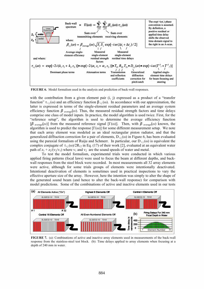
To test the model formalism, experimental trials were conducted in which various applied firing patterns (focal laws) were used to focus the beam at different depths, and back-wall responses from the steel block were recorded. In most measurements all 32 array elements were active, although for some trials groups of elements were intentionally deactivated. Intentional deactivation of elements is sometimes used in practical inspections to vary the effective aperture size of the array. However, here the intention was simply to alter the shape of the generated sound beam (and hence to alter the back-wall response) for comparison with model predictions. Some of the combinations of active and inactive elements used in our tests

)()()(11

ωτωβω ji

N

jji

N

i∑∑==

=Γ

Z1

Linear Phased-Array

Z2

water

solid where:

Average single-element efficiency

Measured single-element

residual strength factors


residual time delaysand where:

Dominant phase terms Attenuation terms Transmission and reflection coefficients

Applied single-element time delays

for beam focusing and steering

Generalized diffraction

correction for pitch/catch

Back-wall spectrum =

Sum over transmitting elements

Sum over receiving elements

The exp(+iωt.) phase convention is assumed. By definition, a positive residual or applied time delay shifts the observed time-domain signal to the right in an A-scan.]2/)(exp[)()( jijiaverageji ttiSS Δ+Δ−= ωωβωβ

)](exp[)()](2exp[)](2exp[)( 21221222112211 jA

iA

jiji TTiDTRTzzzkzki +−•••+−•+−= ωωααωτ

)()()(11

ωτωβω ji

N

jji

N

i∑∑==

=Γ

Z1

Linear Phased-Array

Z2

water

solidZ1

Linear Phased-Array

Z2

water

solid where:

Average single-element efficiency


residual strength factors


residual time delaysand where:

Dominant phase terms Attenuation terms Transmission and reflection coefficients

Applied single-element time delays

for beam focusing and steering

Generalized diffraction

correction for pitch/catch

Back-wall spectrum =

Sum over transmitting elements

Sum over receiving elements

The exp(+iωt.) phase convention is assumed. By definition, a positive residual or applied time delay shifts the observed time-domain signal to the right in an A-scan.]2/)(exp[)()( jijiaverageji ttiSS Δ+Δ−= ωωβωβ

)](exp[)()](2exp[)](2exp[)( 21221222112211 jA

iA

jiji TTiDTRTzzzkzki +−•••+−•+−= ωωααωτ

FIGURE 6. Model formalism used in the analysis and prediction of back-wall responses.

5L32E32-10 T018

5L32E32-10 T018

All Elements Active (“On”)

5L32E32-10 T018

Central 4 Elements Off

5L32E32-10 T018

Highest 8 Elements Off

5L32E32-10 T018

Central 16 Elements Off All Even-Numbered Elements Off

# 32# 1Firing Delays For 240 mm

Focal Depth in Water

4002000

Element NumberTim

e de

lay

in

nano

seco

nds

(a)

(b)

5L32E32-10 T0185L32E32-10 T018

5L32E32-10 T0185L32E32-10 T018

All Elements Active (“On”)

5L32E32-10 T018


5L32E32-10 T0185L32E32-10 T018


5L32E32-10 T018


5L32E32-10 T018


5L32E32-10 T018


5L32E32-10 T0185L32E32-10 T018

Central 16 Elements Off All Even-Numbered Elements Off

# 32# 1Firing Delays For 240 mm

Focal Depth in Water

4002000

Element NumberTim

e de

lay

in

nano

seco

nds

Firing Delays For 240 mm Focal Depth in Water

4002000

Element NumberTim

e de

lay

in

nano

seco

nds

(a)

(b)

FIGURE 7. (a): Combinations of active and inactive array elements used in measurements of the back-wall response from the stainless-steel test block. (b): Time delays applied to array elements when focusing at a depth of 240 mm in water.

884


are shown in Figure 7. Typical comparisons of measured and modeled back-wall responses are summarized in

Figure 8. For each group of comparisons, Figure 8a indicates the nature of the measurements and the source of the reference signal that was analyzed to deduce the average efficiency function. The next three panels (Figures 8b-8d) compare the spectral magnitudes of measured (solid curves) and predicted (plotted points) back-wall responses. For the results in Figure 8b all 32 elements were active, but the focal distance was changed by altering the applied time delays for the array elements. For an unfocused beam, the applied time delays (TA

j in Figure 6) are all set to zero. For a positive focal length, the applied time delays are such that elements near the center of the transducer fire later than those near the edges. For one case, namely a geometric focal depth of 240 mm in water, Figure 7b displays the applied time delays for each element; these range from from 0 nsec for outer elements #1 and #32 to 337 nsec for inner elements # 16 and # 17.

FIGURE 8. Comparisons of measured and predicted back-wall responses for the stainless steel test block. (a): Descriptions of the various measurements, including the nature of the reference signal for each test trial. (b)–(d): Comparisons of measured and predicted back-wall spectra. (e): Comparisons of measured and predicted time-domain signals for three of the cases.

Test 3. F = 240 mm Focal Depth Various Groupings of Active Elements

0.0

1.0

2.0

3.0

4.0

5.0

6.0

7.0

0 1 2 3 4 5 6 7 8 9 10

Frequency (MHz)

Spe

ctru

m M

agni

tude

All onCenter 4 offHigh 8 offCenter 16 offAll evens offAll onCenter 4 offHigh 8 offCenter 16 offAll evens off

Solid curves are exper.

Plotted points are model.

Test 2. F = 240 mm Focal Depth Various Groupings of Active Elements

0.0

1.0

2.0

3.0

4.0

5.0

6.0

7.0

0 1 2 3 4 5 6 7 8 9 10

Frequency (MHz)

Spe

ctru

m M

agni

tude

All onCenter 4 offHigh 8 offCenter 16 offAll evens offAll onCenter 4 offHigh 8 offCenter 16 offAll evens off



Test 1. Back-Wall Spectra For Various Choices of the Focal Depth

0.0

1.0

2.0

3.0

4.0

5.0

6.0

7.0

0 1 2 3 4 5 6 7 8 9 10

Frequency (MHz)

Spe

ctru

m M

agni

tude

F = 10000 mmF = 500 mmF = 240 mmF = 200 mmF = 175 mmF = 10000 mmF = 500 mmF = 240 mmF = 200 mmF = 175 mm



Back-wall echo when focused on back wall (F =240 mm). All “on”.

Test 3

Unfocused back-wall echo. All “on”.

Test 2

Back-wall signals for various focal lengths. All elements “on”.

Unfocused back-wall echo. All elements “on”.

Test 1

What was measured ?Reference SignalTest

Back-wall echo when focused on back wall (F =240 mm). All “on”.

Test 3

Unfocused back-wall echo. All “on”.

Test 2

Back-wall signals for various focal lengths. All elements “on”.

Unfocused back-wall echo. All elements “on”.

Test 1

What was measured ?Reference SignalTest

Measured and Predicted Spectra for Various Experiments Using a 32-Element, Linear,

Phased-Array Transducer(b)

(c) (d)

Back-wall signal when focused on the back-wall (F =240 mm). Various element groups “on” or “off”

(a)

Back-Wall Response; Test 1. F = 240 mm. All Elements Firing

-0.50-0.40-0.30-0.20-0.100.000.100.200.300.40

83 84 85 86 87

Arrival Time (microsec)

RF

Res

pons

e (V

olts

)

Focus at 240mm (Exp)Focus at 240mm (Thry)

Back-Wall Response; Test 1. F = 175 mm. All Elements Firing.

-0.40

-0.30-0.20

-0.10

0.00

0.100.20

0.30

0.40

83 84 85 86 87


Focus at 175mm (Exp)Focus at 175mm (Thry)

Back-Wall Response; Test 3. F = 240 mm. High 8 Elements Off.

-0.40

-0.30-0.20

-0.10

0.00

0.100.20

0.30

0.40

83 84 85 86 87


High 8 off (Exp)High 8 off (Thry)

(e)

885


The various applied focal lengths in water are labeled in Figure 8 and range from 175 mm to 10000 mm. As the focal length is systematically decreased from F = 10000 mm, the back-wall response first drops and then rises, achieving it maximum value when the beam is focused on the steel back wall (near F = 240 mm for our 50 mm water path). As the focal length is decreased further, the back-wall response again drops. In general, as may be seen in Figure 8b, the effect on the back-wall response of varying the focal length was found to be well predicted by the model formalism.

For a fixed focal length of 240 mm in water, Figures 8c-d display how the back-wall response varied as groups of elements were switched off. Predicted responses are shown for two choices of the measured reference signal having different focal conditions (unfocused beam or beam focused near the back wall). As expected, as more elements were turned off the amplitude of the back-wall response dropped, with the details of the drop depending on the number and locations of the inactive elements. Again model predicted spectra were found to be in good agreement with measurement. As illustrated in Figure 8e, time-domain waveforms for back-wall responses were also well-predicted by the model, with measured and predicted peak-to-peak voltages typically agreeing to within about +/- 5%. The average grain size in this steel specimen is fairly large (about 90 microns [3]), and earlier measurements with 5-MHz fixed-focused transducers found back-wall-amplitude variations with position (“speckle”) of about +/- 5%. Thus some of the difference between measured and predicted back-wall responses in Figure 8 is likely due to microstructure-induced signal fluctuations. SUMMARY

The method proposed here for system efficiency determination allows one to take element-to-element differences into account, but to still employ a single measured reference signal at the time of an inspection, as is the case for fixed-focus transducers. In experimental trials using a 5-MHz linear phased-array transducer and a stainless steel block, good agreement was found between measured and predicted back-wall responses. The method makes use of residual strength and time delay parameters which are measured (on an occasional basis) for each array element individually. We note that many phased-array pulse/receiver instruments allow both gains and time delays to be set independently for each array element. Given knowledge of the residual parameters defined here, such a capability could be used to largely “correct” transducer operating characteristics for the element-to-element differences.

ACKNOWLEDGEMENT

This material is based upon work supported by the Air Force Research Laboratory under Contract # FA8650-04-C-5228 at Iowa State University's Center for NDE. REFERENCES 1. R.B. Thompson and T.A. Gray, “A model relating ultrasonic scattering measurements

through liquid-solid interfaces to unbounded medium scattering amplitudes”, Journal of the Acoustical Society of America 74 (1983), pp. 1279–1290.

2. Ruiju Huang and Lester W. Schmerr Jr. , “Characterization of the system functions of ultrasonic linear phased array inspection systems”, Ultrasonics, 49, February 2009, pp. 219-225.

3. F. J. Margetan, T. A. Gray and R. B. Thompson, “Measurement and Modeling of Ultrasonic Pitch/Catch Grain Noise”, Rev. of Prog. in QNDE, 27B, eds. D.O. Thompson and D.E. Chimenti, (AIP, Melville NY, 2008), pp.1132-1139. (The steel specimen whose properties are described in this reference is the same one used in the present study).

886


simplified system efficiency functions for linear phased-array … · 2017-05-03 · simplified...

Documents