simplified control strategies for modular multilevel
TRANSCRIPT

Simplified Control Strategies for Modular
Multilevel Matrix Converter for Offshore
Low Frequency AC Transmission System
Jiankai Ma
A thesis submitted for the degree of
Doctor of Philosophy
September, 2018
School of Engineering
Newcastle University
United Kingdom


i
Abstract
The Low frequency AC (LFAC) transmission system is considered as the most cost-saving
choice for the short and intermediate distance. It not only improves the transmission capacity
and distance but also has higher reliability which makes it more advantageous than the HVDC
transmission system. Modular Multilevel Matrix Converter (M3C) is recognized as the most
suitable frequency converter for the LFAC transmission system which is responsible for
connecting 16.7 Hz and 50 Hz ac systems. In such applications, the ‘double αβ0 transform’
control method is most popular technique that realizes the decoupled control of the input current,
output current and circulating current. However, the derivation process of the mathematical
model is so complicated that it gives too much burden on the controller of the M3C system.
Therefore, this thesis is focusing on simplifying the M3C control strategies when used in LFAC
systems and the primary contribution to the knowledge is outlined as follows:
(1) A simplified hierarchical energy balance control method which employs an independent
control for each of three sub-converters in M3C is proposed in Chapter 5. The output
frequency circulating current is injected and utilized to balance the energy between the three
arms of the sub-converter. The proposed method achieves a reduced execution time and a
simplified control structure, with which a low-cost processor is applicable and the control
bandwidth of the system is improved.
(2) An improved energy balance control method with injecting both input and output frequency
circulating currents is proposed in Chapter 6. The magnitudes of the circulating current
responsible for the energy balance control in either frequency are half reduced as compared
to the single frequency injection method in Chapter 5. This arrangement alleviates the
negative impact of the injected circulating current on the external grid and allows the M3C
systems work through larger grid unbalance situations.
Finally, the effectiveness of the proposed control strategy is demonstrated by extensive
simulation results and validated experimentally using a scaled-down laboratory prototype.

ii

iii
Contents
Chapter 1 Introduction .................................................................................................... 1
1.1 Motivation and objectives .................................................................................. 1
1.2 Contribution to knowledge ................................................................................... 3
1.3 List of publications ............................................................................................... 4
1.4 Thesis overview .................................................................................................... 4
Chapter 2 Literature Review ........................................................................................... 6
2.1 Transmission systems for the offshore wind farm ................................................ 6
2.1.1 High-voltage Alternating-current (HVAC) transmission system ............... 7
2.1.2 High-voltage Direct-current (HVDC) transmission system ...................... 7
2.1.3 Low Frequency AC (LFAC) transmission system ...................................... 9
2.2 The Modular Multilevel Converters family ........................................................ 11
2.2.1 Multilevel Converters .............................................................................. 11
2.2.2 The Modular Multilevel Converters family ............................................. 13
2.3 The Overview of M3C ........................................................................................ 17
2.3.1 The history of M3C ................................................................................... 17
2.3.2 The modeling and arm power analysis for M3C ...................................... 19
2.3.3 Capacitor voltage balance control strategy of M3C ................................ 20
2.3.4 Research on special working conditions of M3C ..................................... 21
2.3.5 Research on the failure operation of M3C ............................................... 22
2.4 Summary ............................................................................................................. 23
Chapter 3 Modelling and Analysis of Modular Multilevel Matrix Converter .............. 24
3.1 Circuit topology of M3C ..................................................................................... 24
3.2 The mathematical model of M3C ........................................................................ 25
3.3 The mathematical model of sub-module in M3C ................................................ 26
3.4 The spectrum analysis of the M3C arm instantaneous power ............................. 30
3.5 Illustrative simulation results.............................................................................. 33
3.5.1 The selection of capacitor and arm inductor .......................................... 34
3.5.2 FFT Analysis of the capacitor voltage and the arm current .................... 34
3.6 Summary ............................................................................................................. 36
Chapter 4 The ‘double αβ0 transformation’ control method of M3C ............................ 37
4.1 The mathematical model of M3C based on αβ0 frame ....................................... 37
4.2 Power analysis based on αβ0 frame.................................................................... 39

iv
4.2 The ‘double αβ0 transformation’ control method ............................................... 40
4.2.1 Capacitor voltage control ........................................................................ 41
4.2.2 Input, output and circulating current control .......................................... 44
4.3 Illustrative simulation results under output voltage step change operation........ 47
4.3.1 Case I: Steady state operation ................................................................. 47
4.3.2 Case II: Dynamic output power operation .............................................. 48
4.4 Summary ............................................................................................................. 49
Chapter 5 Hierarchical Energy Balance Control Method for M3C based on Injecting
Output Frequency Circulating Currents ................................................................................... 50
5.1 The mathematical model of sub-converter a ...................................................... 50
5.2 The proposed control strategy ............................................................................ 52
5.2.1 Sub-converter Energy Balance Control ................................................... 52
a. Active and Reactive Power Control .......................................................... 53
b. Overall capacitor voltage control ............................................................ 54
5.2.2 Energy Balance Control between the three arms of the sub-converter
(Capacitor voltage balancing control) ..................................................................... 55
5.2.3 The arm current Control .......................................................................... 58
5.2.4 Energy balance control between n SMs of each arm (Selective Voltage
Mapping Modulation) ............................................................................................... 58
5.3 Illustrative Simulation Results ........................................................................... 60
5.3.1 Case I: Steady-state operation ................................................................ 61
5.3.2 Case II: Dynamic output power operation .............................................. 62
5.3.3 Case III: Unbalanced grid voltage condition .......................................... 63
5.4 Summary ............................................................................................................. 64
Chapter 6 Hierarchical Energy Balance Control Method for M3C based on Injecting
Two Frequency Circulating Currents ....................................................................................... 66
6.1 Circuit topology of M3C ..................................................................................... 66
6.2 The mathematical model of M3C ........................................................................ 67
6.3 The Proposed control strategy ............................................................................ 69
6.3.1 Energy balance control of M3C ............................................................... 70
6.3.2 Energy balance control between the three arms in the sub-converter A
(circulating current control) ..................................................................................... 72
6.3.3 Energy balance control between three arms of the sub-converter a
(circulating current control) ..................................................................................... 75

v
6.3.4 The arm current control ........................................................................... 78
6.3.5 Energy balance control between n SMs of each arm (SVMM) ................ 79
6.4 Illustrative simulation results.............................................................................. 79
6.4.1 Case I: Steady-state operation ................................................................ 79
6.4.2 Case II: Dynamic output power operation .............................................. 80
6.5 Comparison between the ‘double αβ0 transformation’ control method and
proposed control methods ................................................................................................. 81
6.6 Summary ............................................................................................................. 83
Chapter 7 Experimental Validation ............................................................................... 84
7.1 Experimental setup ............................................................................................. 84
7.2 Design and function of M3C prototype .............................................................. 85
7.2.1 Distributed control network of M3C prototype ........................................ 85
7.2.2 Communication Network ......................................................................... 88
7.2.3 The design of the software for the distributed control network of M3C .. 92
7.3 The design of the arm board of M3C .................................................................. 92
7.4 The design of the full-bridge sub-module .......................................................... 94
7.5 Experimental Results .......................................................................................... 97
7.5.1 The design of the pre-charge and soft-start process of the prototype ...... 98
7.5.2 The experimental results of the Hierarchical Energy Balance Control
Method for M3C based on Injecting Output Frequency Circulating Currents ......... 99
7.5.3 The experimental results of the Hierarchical Energy Balance Control
Method for M3C based on Injecting Two Frequency Circulating Currents ........... 105
7.6 Summary ........................................................................................................... 109
Chapter 8 Conclusions and Future Work .................................................................... 110
8.1 Conclusions ...................................................................................................... 110
8.2 Future work ...................................................................................................... 111
Reference ........................................................................................................................ 113

vi
List of Figures
Figure 2.1 Main components of an offshore wind farm: (a) Wind turbines (b) Collection
cables (c) Export cables (d) Transformer station (e) Converter station (f)
Meteorological mast (g) Onshore stations[1] ............................................................... 6
Figure 2.2 Three major offshore transmission systems ...................................................... 6
Figure 2.3 Typical layout of the HVAC transmission system for offshore wind farm ....... 7
Figure 2.4 Typical layout of the HVDC transmission system for offshore wind farm ...... 8
Figure 2.5 Investment for three offshore transmission systems ......................................... 9
Figure 2.6 The LFAC transmission system based on conventional wind turbines ........... 10
Figure 2.7 The LFAC transmission system based on re-designed wind turbines ............. 10
Figure 2.8 (a) Three-level NPC (b) Four-level FC ........................................................... 12
Figure 2.9 Categories of the multilevel converters........................................................... 13
Figure 2.10 (a) Half-bridge SM (b) Full-bridge SM (c) Clamp double SM ..................... 14
Figure 2.11 (a) Five-level cross-connected SM (b) Unipolar-voltage full-bridge SM ..... 15
Figure 2.12 Members of the Modular Multilevel Converters family ............................... 16
Figure 2.13 (a) Conventional matrix converter (b) First published structure of M3C ...... 18
Figure 2.14 Circuit diagram of the M3C with an arm inductor ........................................ 19
Figure 3.1 The circuit diagram of Modular Multilevel Matrix Converter ........................ 24
Figure 3.2 Circuit diagram of sub-converter a in M3C ..................................................... 25
Figure 3.3 Circuit diagram of the SM in sub-converter a of M3C .................................... 27
Figure 3.4 Status of SM in M3C ....................................................................................... 28
Figure 3.5 Status of SM in M3C ....................................................................................... 28
Figure 3.6 Status of SM in M3C ....................................................................................... 29
Figure 3.7 Status of SM in M3C ....................................................................................... 29
Figure 3.8 The linear steady state model of the armxa ...................................................... 30
Figure 3.9 The relationship between the frequency ratio and the capacitor voltage ripple[95]
.................................................................................................................................. 32
Figure 3.10 (a) Capacitor voltage (b) FFT analysis of the capacitor voltage ................... 35
Figure 3.11 (a) Arm current (b) FFT analysis of the arm current ..................................... 36

vii
Figure 4.1 The block diagram for the ‘double αβ0 transformation’ control ..................... 41
Figure 4.2 The overall capacitor voltage control block diagram ...................................... 42
Figure 4.3 The capacitor voltage balancing control block diagram ................................. 44
Figure 4.4 The block diagram of the input current control .............................................. 45
Figure 4.5 The block diagram of the output current control ............................................ 46
Figure 4.6 The block diagram of the circulating current control ...................................... 46
Figure 4.7 Simulation results under the steady-state operation ........................................ 48
Figure 4.8 Simulation results under a dynamic output power operation .......................... 49
Figure 5.1 The circuit diagram of Modular Multilevel Matrix Converter ........................ 50
Figure 5.2 The block diagram of the proposed control method in sub-converter a ......... 52
Figure 5.3 Active and reactive power control block diagram .......................................... 53
Figure 5.4 The block diagram of the overall capacitor voltage control ........................... 54
Figure 5.5 The block diagram of the capacitor voltage balancing control in sub-converter
a ................................................................................................................................ 56
Figure 5.6 One possible power exchange path ................................................................. 57
Figure 5.7 Arm current control block diagram ................................................................. 58
Figure 5.8 (a) Full bridge SM (b) PWM signals of five SMs ........................................... 59
Figure 5.9 PWM signals mapping of SVMM .................................................................. 60
Figure 5.10 Simulation results under steady-state operation ............................................ 62
Figure 5.11 Simulation results under a dynamic output power operation ........................ 63
Figure 5.12 Simulation results under unbalanced grid voltage condition ........................ 64
Figure 6.1 Circuit diagram for M3C divided into sub-converters a, b and c .................... 66
Figure 6.2 Circuit diagram for M3C divided into sub-converters A, B and C .................. 67
Figure 6.3 The block diagram of the proposed control method in sub-converter a and sub-
converter A ............................................................................................................... 70
Figure 6.4 Active and reactive power control block diagram .......................................... 71
Figure 6.5 The overall capacitor voltage control block diagram ...................................... 71
Figure 6.6 The block diagram of the capacitor voltage balancing control in sub-converter
A ............................................................................................................................... 73

viii
Figure 6.7 An example power exchange path (a) Sub-converter A (b) Sub-converter a, b
and c .......................................................................................................................... 74
Figure 6.8 The block diagram of the capacitor voltage balancing control in sub-converter
a ................................................................................................................................ 76
Figure 6.9 An example power exchange path (a) Sub-converter a (b) Sub-converter A, B
and C ......................................................................................................................... 77
Figure 6.10 Arm current control block diagram ............................................................... 78
Figure 6.11 Simulation results under steady-state operation ............................................ 80
Figure 6.12 Simulation results under dynamic output power operation........................... 81
Figure 6.13 Comparison of the mathematical calculation between three control methods
.................................................................................................................................. 82
Figure 6.14 Comparison of the operation time between three control methods............... 82
Figure 7.1 Experiment platform of the three phase to three phase M3C .......................... 84
Figure 7.2 The distributed control network of M3C ......................................................... 85
Figure 7.3 Function of the master controller .................................................................... 86
Figure 7.4 Function of the arm controller ........................................................................ 87
Figure 7.5 The distributed control network of M3C in details.......................................... 87
Figure 7.6 Four typical structures of the communication network................................... 88
Figure 7.7 The distributed control network (ring structure) based on EtherCAT for MMC
.................................................................................................................................. 89
Figure 7.8 Structure of the CAN bus in the distributed control network of M3C ............ 90
Figure 7.9 Schematic of the CAN interface ..................................................................... 91
Figure 7.10 The communication of the distributed control network by using CAN ........ 91
Figure 7.11 The design of the software for the distributed control network of M3C ....... 92
Figure 7.12 (a) Circuit diagram of the arm in M3C (b) The arm board ............................ 93
Figure 7.13 Schematic of the DSP controller ................................................................... 93
Figure 7.14 Schematic of the full-bridge SM in M3C ...................................................... 94
Figure 7.15 Inner schematic and peripheral circuit of DIPIPM ....................................... 94
Figure 7.16 Feedback circuit of the fault signal ............................................................... 96

ix
Figure 7.17 The relationship between input current and output voltage of hall voltage
sensor ........................................................................................................................ 96
Figure 7.18 Sampling and processing circuit of the capacitor voltage ............................. 97
Figure 7.19 An example current flow path at the uncontrolled rectifier stage ................. 98
Figure 7.20 Experimental results of the pre-charge and soft-start process ...................... 99
Figure 7.21 Experimental results under steady-state operation ...................................... 100
Figure 7.22 The simulation results of arm current and the corresponding FFT analysis
when fi=16.7 Hz and fo=50 Hz ................................................................................ 101
Figure 7.23 The simulation results of arm current and the corresponding FFT analysis
when fi=50 Hz and fo=16.7 Hz ................................................................................ 102
Figure 7.24 Simulation results of the proposed control method when fi=50 Hz and fo=16.7
Hz ........................................................................................................................... 103
Figure 7.25 Experimental results under output frequency step change operation.......... 104
Figure 7.26 Experimental results under output voltage step change operation .............. 105
Figure 7.27 Experimental results under steady-state operation ...................................... 106
Figure 7.28 Experimental results under output frequency step change operation.......... 107
Figure 7.29 Experimental results under output voltage step change operation .............. 108

x
List of Tables
Table 3.1 Switching states of SM in M3C ........................................................................ 27
Table 3.2 Simulation parameters ...................................................................................... 33
Table 4.1 Simulation parameters of the proposed control method ................................... 47
Table 6.1 The relationship between nine arms and six sub-converters ............................ 67
Table 7.1 Experimental parameters of the proposed control methods ............................. 97

xi
Acronyms and symbols
List of Symbols
P Rated active power
Ei Input phase RMS voltage
fi Input frequency
Li Input inductance
Eo Output phase RMS voltage
fo Output frequency
Lo Output inductance
Ro Load Resistance
L Arm inductance
Lg Grid-connected filter inductance
Cg Grid-connected filter capacitance
fs Switching frequency
Cxyz Capacitance of SM’s capacitor
UCxyz* Rated dc capacitor voltage
n Number of SMs per arm
eα_i, eβ_i Input voltage in the αβ0 frame
eα_o, eβ_o Input voltage in the αβ0 frame
uαα, uβα, …, u00 Nine arm voltages in the αβ0 frame
iαα, iβα, …, i00 Nine arm currents in the αβ0 frame
Le Equivalent inductance
pαα, pβα, …, p00 Nine arm power in the αβ0 frame
UCαα, UCβα, …, UC00 DC capacitor voltages in the αβ0 frame
pi Input power
po Output power
id_i, iq_i Input current in the dq frame
K1, K2, …, K6 Proportional gain
Tabc/αβ0, [Tabc/αβ0]T, Tabc/dq, Tdq/abc Transformation matrix

xii
iαα, iβα, iαβ, iββ Circulating current in the αβ0 frame
ωo Angular frequency of the output side
ωi Angular frequency of the input side
φA
relative phase angle of the input current wrt the input
voltage
φa relative phase angle of the output current wrt the
output voltage
θ Rotating frequency of the input or output grid
voltage
θi Rotating frequency of the input grid voltage
θo Rotating frequency of the output grid voltage
EA, EB, EC RMS value of the input voltages
IA, IB, IC RMS value of the input current
Ea, Eb, Ec RMS value of the output voltage
Ia, Ib, Ic RMS value of the output current
armxy Each arm in M3C
ixy Output current of the corresponding arm
uxy Output voltage of the corresponding arm
uxyz Output voltage of each SM
ixy_i Input current component
ixy_o Output current component
ixy_cir Circulating current component
ixy_cir_i Circulating current component with input frequency
ixy_cir_o Circulating current component with output frequency
uCxyz Capacitor voltage of each SM
uxyz Output voltage of each SM
iCxyz Current go through the capacitor of each SM
ixyz Output current of each SM
uxy Arm voltage

xiii
uCxy Sum of capacitor voltages of the corresponding arm
pCxy Active power of each SM
pxy Arm power
wxy Arm’s energy
UCxy DC capacitor voltage
xaCu Capacitor voltage ripple
ε Percentage of the capacitor voltage ripple
△i Maximum ripple of the arm current
k Eo/ Ei
h Io/ Ii
λ ωo/ωi
List of acronyms
M3C Modular Multilevel Matrix Converter
LFAC Low Frequency AC transmission system
HVAC High voltage AC transmission system
HVDC High voltage DC transmission system
AC Alternating current
DC Direct current
SVMM Selective voltage mapping modulation
MMC Modular Multilevel Converter
SM Sub-module
CHBC Cascaded H-bridge converter
LCC Line commutated converter
VSC Voltage source converter
IGBT Insulated gate bipolar transistor
FFTS Fractional frequency transmission system
THD Total Harmonic distortion
NPC Neutral point clamped converter

xiv
FC Flying capacitor converter
STATOCM Static synchronous compensator
UPFC Unified power flow controller
SVM Space vector modulation
PI Proportional integral
PWM Pulse width modulation
FCS-MPC Finite control set-model predictive control
DSP Digital signal processor
FPGA Field-Programmable Gate Array
CAN Controller area network

Chapter 1 Introduction
1
Chapter 1 Introduction
1.1 Motivation and objectives
Energy shortage, climate warming and environmental degradation have become the biggest
public crises for the sustainable development of human society. Therefore, the transformation
to green and low-carbon structure with clean energy and emission reduction has become the
priority of all countries in the world. The UK government has set a goal for the deployment of
renewable energy for the next decade which is that 20% of the UK’s total energy should come
from renewable sources [1]. Typically, due to geographic problem and the rapid growing
capacity of wind farm. A wind farm is normally very far away from the major power grid or
load centers. Considering these cases, the transmission of wind power from remote offshore
wind farm has been raised as an important issue. The main task is exploring the way to increase
transmission distance and capacity.
Apart from the traditional High voltage AC (HVAC) transmission system and the mature High
voltage DC (HVDC) transmission system, the Low Frequency (16.7 Hz) AC (LFAC)
transmission system is considering as the solution for the future development of offshore wind
farm. The LFAC transmission system has two main advantages: 1) Compared with the HVAC
transmission system, the low frequency reduced the charging current which provides higher
transmission capacity and longer transmission distance; 2) Compared with the HVDC
transmission system, the construction and maintenance cost less since there is only one onshore
ac/ac converter for the LFAC transmission system [2].
The onshore ac/ac converter is obviously the most important part of the LFAC transmission
system. The most commonly used frequency converter is the cycloconverter. However, it
suffers from the heavy harmonics and low power factors which limits its future development
[3]-[4]. The Modular Multilevel Matrix Converter (M3C) has been recognized as the next
generation of the ac/ac converter, with merits of high flexibility and scalability, high power
quality and being able to control both sides’ power factor, but the control of M3C brings
difficulty for the application to the LFAC transmission system.
Chapter 1 Introduction
2
There are eight current degrees of freedom and nine voltage degrees of freedom in M3C. Two
frequency components from both sides of the ac networks within the arm current cause highly
coupled relationship between these degrees of freedom and brings the main challenge in
controlling M3C. The commonly used mathematical model of M3C is based on the ‘double αβ0
transformation’ control method which was proposed in [5] where the control algorithm is
designed based on the sophisticated mathematical calculation which requires multiple αβ0
transformations to decouple the input current, output current and circulating current. It results
in a very complex analysis of the mathematical relationship between the arm power and the
capacitor voltage. According to that mathematical relationship, the circulating current which
contains both input and output frequency components is used to balance the capacitor voltage.
Reference [6] proposed the ‘dq transformation’ control method based on [5] where the current
is transformed to dq axis dc signals for a better performance. The capacitor voltage fluctuations
of M3C is significant when the input/output frequency get close to each other. In order to solve
this problem, reference [7] reallocates the arm currents by only using inner circulating currents.
However, this control method is also developed from [5]. A generalized control method for
Modular Multilevel Converter topologies (MMC, M3C etc.) is proposed in [8]. It presents a
current control based on the state-space representation and an optimized arm energy balancing
control which has been applied to M3C as an example. It concluded that reference [5] are
boundary cases of their proposed control method and their method has better performance.
However, these two methods both need a very complex control algorithm and associated
mathematical calculation. Reference [9] proposed the method which decouples the sub-
converter currents into positive, negative and zero sequences in order to control the input
current, circulating current and output current independently. It uses the negative sequence
circulating current, which is running at the input frequency, to balance the inter-arm dc-link
voltages within each sub-converter. This idea is similar to the commonly used “negative
sequence current injection” methods in the star-connected cascaded H-bridge converters
(CHBC) [10]. Several predictive control methods are also developed for M3C such as [11].
However, predictive control method needs accurate system parameters and a huge amount of
real time calculation which makes it less practical.

Chapter 1 Introduction
3
The focus of this thesis is on the design of the control algorithm for M3C. The simplification of
the inter-arm dc-link capacitor voltage balancing control reduced the control complexity and
the associated mathematical calculation. More specifically, three main research objectives are
as follows:
⚫ Investigate and identify the relationship between the eight current degrees of freedom and
nine voltage degrees of freedom in M3C. Quantify the mathematical relationship between
the arm power and capacitor voltage which is the major energy balance control elements;
⚫ Design the control algorithm which should not be developed from the commonly used
control method to balance the capacitor voltage. The injection of the circulating current
should be designed without affecting the input/output side.
⚫ Validate the proposed control methods using an ‘close-to-reality’ simulation model and a
real-time three phase-to-three phase M3C (three sub-modules in each arm) laboratory test
bench.
1.2 Contribution to knowledge
The original contributions of this research work are concluded as follows:
⚫ A simplified hierarchical energy balance control method with injecting output frequency
circulating current in proposed in Chapter 5 to achieve an independent sub-converter
control of M3C. The circulating current control has been designed easily and accurately for
the purpose of compensating the energy difference between the three arms of each sub-
converter. The complexity and associated mathematical calculation has been dramatically
reduced compared with earlier methods proposed in the literature, achieving a reduced
execution time and a simplified control structure, so that a low-cost processor is applicable
and the control bandwidth of the system is improved. Experimental results confirm the
simulation results and further demonstrated a comparable performance with other relevant
papers presented in the literature.
⚫ An improved energy balance control method with injecting both input and output frequency
circulating currents is proposed in Chapter 6. The magnitudes of the circulating current
responsible for the energy balance control in either frequency are half reduced as compared

Chapter 1 Introduction
4
to the single frequency injection method in Chapter 5. This arrangement alleviates the
negative impact of the injected circulating current on the external grid and allows the M3C
systems work through larger grid unbalance situations.
Furthermore, a distributed hardware control structure of the M3C system is proposed in Chapter
7 to experimentally validate the effectiveness of the proposed two control strategies. This
hardware structure is on the basis of the distributed local processor which further alleviates the
control burden of the master controller.
1.3 List of publications
The early research has been published as conference papers and further research based on that
is written as one journal paper which has been submitted to the power electronics.
[C1] J. Ma, M. Dahidah, V. Pickert and J. Yu, " Simplified Hierarchical Energy Balance Control
Method for M3C with Frequency Decoupling Strategy," submitted to the IEEE Transactions on
Power Electronics.
[J1] J. Ma, M. Dahidah, V. Pickert and J. Yu, "Modular multilevel matrix converter for offshore
low frequency AC transmission system," 2017 IEEE 26th International Symposium on
Industrial Electronics (ISIE), Edinburgh, 2017, pp. 768-774.
[C2] J. Liu, W. Yao, Z. Lu and J. Ma, "Design and implementation of a distributed control
structure for modular multilevel matrix converter," 2018 IEEE Applied Power Electronics
Conference and Exposition (APEC), San Antonio, TX, 2018, pp. 1934-1939.
1.4 Thesis overview
A brief description of each chapter is as follows: Chapter 2 reviewed three transmission systems
for offshore wind farm. M3C which function as the frequency converter is also reviewed in
terms of its history of and various control methods. Chapter 3 presents the circuit topology and
the mathematical model of the proposed M3C with the spectrum analysis of its arm power.
Chapter 4 presents the most commonly used control method of M3C which is names as ‘double
αβ0 transformation’ control method. Chapter 5 proposed a simplified hierarchical energy
balance control method of M3C with injecting output frequency circulating current. Chapter 6

Chapter 1 Introduction
5
proposed an improved energy balance control method with injecting both input and output
frequency circulating currents. Chapter 7 presented the experimental validation based on a
small laboratory prototype. Finally, Chapter 8 concluded the work and presented the
recommendations for the future work.

Chapter 2 Literature Review
6
Chapter 2 Literature Review
2.1 Transmission systems for the offshore wind farm
Different with onshore wind farms, the offshore wind farm requires the submarine cables to
transmit electricity to the onshore grid. Figure 2.1 presents a typical structure of the offshore
wind power station [12].
Figure 2.1 Main components of an offshore wind farm: (a) Wind turbines (b) Collection cables (c) Export
cables (d) Transformer station (e) Converter station (f) Meteorological mast (g) Onshore stations[1]
Since the cable length and the transmission voltage are determined by the distance and the rated
power of the offshore wind farm, the only variable is the frequency. Currently, there are three
major transmission technologies as illustrated Figure 2.2: High-voltage Alternating-current
(HVAC) transmission system, High-voltage Direct-current (HVDC) transmission system and
Low frequency AC (LFAC) transmission system.
Wind Farm
AC/DC
AC/AC
DC/AC
Grid
HVDC
LFAC
HVAC50 Hz
16.7 Hz
50 Hz
50 Hz
50 Hz
50 Hz
Offshore Onshore
Figure 2.2 Three major offshore transmission systems

Chapter 2 Literature Review
7
2.1.1 High-voltage Alternating-current (HVAC) transmission system
The High-voltage Alternating-current (HVAC) transmission system (operating at 50Hz or 60Hz)
is the common choice because of its simplicity of construction [13]. Figure 2.3 shows the typical
layout of the HVAC transmission system for offshore wind farm. The submarine cables connect
the offshore wind farm and the onshore substation to transmit the electricity.
G
G
Wind turbines
Wind turbines
Offshore
stationSubmarine cable
Offshore
compensationOnshore
compensation
Substation Grid
Figure 2.3 Typical layout of the HVAC transmission system for offshore wind farm
However, the submarine cables’ high parasitic capacitance generates charging current, which
means the reactive power compensation is required before the connection to the grid [14].
Therefore, the HVAC transmission system is less suitable for high capacity offshore wind farm
when the transmission distance is long [15]. In addition, when fault situations happen offshore,
both sides of the HVAC transmission system will be affected, since the onshore grid is directly
connected to the offshore wind farm [16].
2.1.2 High-voltage Direct-current (HVDC) transmission system
Compared with AC transmission technology, DC configurations do not have the charging
current or the need for the reactive power compensation. Hence, the High-voltage Direct-
current (HVDC) transmission system has been regarded as the best solution for the middle to
long range (>150 km) transmission over the last decades. As shown in Figure 2.4, the HVDC
transmission system contains three major components which are the offshore converter
platform, submarine cables and the onshore converter stations.

Chapter 2 Literature Review
8
G
G
Wind turbines
Wind turbines
Submarine
transmission line
Grid
AC
DC
DC
AC
OnshoreOffshore
Figure 2.4 Typical layout of the HVDC transmission system for offshore wind farm
The power converters that have been applied in the HVDC transmission system are usually
divided into two categories: (1) LCC (Line commutated converters) based on thyristors and (2)
VSC (Voltage source converters) based on fully-controllable power switches (such as IGBT).
LCC is a mature technology which has been applied to many transmission systems all over the
world. However it is still important to mention that the LCC requires strong network on both
sides of the converter and additional auxiliary equipment to filter the low-order harmonics [17].
Hence, researchers consider that the HVDC transmission system using LCC is not suitable for
offshore wind farm. Conversely, the VSC-HVDC which utilizes the controllable power device
realizes the independent control of the active power and reactive power with no commutation
failure and low/no extra filter requirement [18]. Although this topology is comparatively new,
it has developed so quickly that many existing projects have adopted the VSC-HVDC
transmission system [18]-[19]. So far, three main topologies in terms of the power converters
are utilized in the VSC-HVDC transmission system: two-level converters, three-level
converters and multilevel converters in order to deal with the high voltage and high power
transmission [20]. However there still exists technical challenges in the VSC-HVDC
transmission system such as the lack of reliable DC circuit breakers and dc/dc transformers [14].
Since an extra converter station needs to be built offshore, it brings many constraints on the
design, manufacture and installation of the offshore platform. Therefore, the VSC-HVDC
transmission system requires quite a large investment in the construction and maintenance.
Some researchers have also stated that the transmission cables have an insulation problem and
shorter life time when carrying DC current [21]-[22].

Chapter 2 Literature Review
9
2.1.3 Low Frequency AC (LFAC) transmission system
In addition to the two transmission schemes presented in the previous sub-sections, there is
another transmission system which is the Low Frequency AC (LFAC) transmission system.
LFAC decreases the transmission frequency to 16.7 Hz thus increasing the transmission
capacity and extending the transmission distance when compared with the HVAC transmission
system. Compared to the HVDC transmission system, it doesn’t need the offshore substation,
and instead requires an AC/AC onshore station to transform the low frequency (16.7 Hz) to the
desired grid frequency (50 Hz) [23]. As a result, this solution does not only deal with the
drawbacks of the HVAC transmission system but also avoids the high investment of the HVDC
transmission system. For short and intermediate distance (30 km-150 km), the LFAC
transmission system is the most cost-competitive choice. However, when the distance increases
further than 150 km, the HVDC transmission system will inevitably become cheaper. Figure
2.5 presents a comparison of investment between the three transmission systems [24]. It should
be noted that Figure 2.5 is illustrative and does not present the exact cost of each transmission
system.
Distance [km]
Investment cost
HVAC
HVDC
LFAC
30 50 150
Figure 2.5 Investment for three offshore transmission systems
In 1994 the Fractional Frequency Transmission System (FFTS) was first proposed to increase
the transmission capacity for remote hydro power plants [25]. Later, a more comprehensive
case study was carried out in [26] which looked at 10000 MW rating wind farms via FFTS. In
2001, the LFAC transmission system was proposed for use in offshore wind farms [27]. Figure
2.6 and Figure 2.7 show two possible designs for LFAC transmission system according to the

Chapter 2 Literature Review
10
different output frequencies of the wind turbines [28]. The design as shown in Figure 2.6 is
based on conventional wind turbines (output frequency: 50 Hz) so it does not require extra
equipment or modifications. However, an offshore power converter does need to be installed to
transform the 50Hz back to the desired low transmission frequency 16.7 Hz.
G
G
Wind turbines
Wind turbines
50Hz
Submarine cable
Grid
AC
AC
OnshoreOffshore
50 Hz
AC
AC
50/3 Hz
Figure 2.6 The LFAC transmission system based on conventional wind turbines
The second topology is presented in Figure 2.7 where the output frequency of the wind turbines
is 16.7 Hz. It means that the offshore frequency converter can be omitted. This largely reduces
the maintenance and control complexity. However, the equipment for the conventional three
phase power system (50 Hz) requires re-qualification and perhaps alterations. At certain power
rating the dimensions of a transformer are inversely proportional to the frequency so that the
magnetic core’s volume for the transformer offshore will be three times larger than the
conventional one [29].
G
G
Wind turbines
Wind turbines
50/3Hz
Submarine cable
Grid
AC
AC
OnshoreOffshore
50 Hz50/3 Hz
Figure 2.7 The LFAC transmission system based on re-designed wind turbines
Different converters have been considered and discussed in the literature and the 6-pulse cyclo-
converter was attempted to triple the frequency in LFAC, from 16.7 Hz to 50 Hz in [30].
Experimental results confirmed its usability but the high total harmonic distortion (THD) makes

Chapter 2 Literature Review
11
it inefficient. A different variation was then presented in [31] where the 6-pulse cycloconverter
is replaced by a 12-pulse cycloconverter aiming to reduce the THD. However, as confirmed by
[32], the 12-pulse cycloconverter still requires large filters to suppress the lower-order
harmonics. Therefore, back-to-back AC-DC-AC converters are considered as an alternative by
researchers instead of the conventional AC-AC converter [33]. The Modular Multilevel
Converter (MMC) is a mature technology in VSC-HVDC, which apparently the back-to-back
arrangement is a good candidate for LFAC system. Reference [34] highlighted that the modular
design of MMC provides capability to meet any voltage level requirements. Meanwhile,
compared with the cycloconverter, it has a superior harmonic performance [35]. However, as
discussed in [30] the structure of the half-bridge sub-module in MMC does not allow clearing
the dc bus short circuit fault, which is a major limitation. As the member of Modular Multilevel
Converter family, M3C which is the research target of this project will be discussed in details
in the later chapters.
2.2 The Modular Multilevel Converters family
2.2.1 Multilevel Converters
Due to the high voltage level of the wind farm, the conventional two-level converters are limited
by the voltage rating of the switching devices. To overcome this limitation, there are two
possible solutions. The first solution is to improve the voltage rating of the switching devices.
For example, this can be achieved by the SiC devices which has been widely researched and
applied or using the high blocking voltage switches made by the series connected small voltage
rating devices. However, this solution introduces extra voltage and current balancing problems
and in addition the high step up voltage will cause the issue of electromagnetic compatibility.
The second solution is to use multilevel topologies which means that the voltage level of the
converter’s output voltage is equal or bigger than three. For example, considering the three-
level neutral point clamped converter (NPC) and the four-level flying capacitor converter (FC)
as shown in Figure 2.8 (a) and (b) [36].

Chapter 2 Literature Review
12
+
_
Vdc
+
_
Vdc
(a) (b)
Figure 2.8 (a) Three-level NPC (b) Four-level FC
Compared with the two-level converter, the multilevel converter reduces the dv/dt of the output
voltage thus decreasing the output’s THD. Meanwhile, the design of the multilevel converter is
very helpful in decreasing the switching frequency and the size of the passive filter. Therefore,
the multilevel converter is the preferred choice for high power applications and has attracted
wide attention in both academic and industrial fields. Figure 2.9 classifies the common
topologies of multilevel converters [37].

Chapter 2 Literature Review
13
Multilevel
converter
Neutral point
clampedFlying capacitor
Cascaded
topologiesHybrid topologies
Transistor clamped
converter
3 Level-Active
Neutral point
clamped
5 Level-Active
Neutral point
clamped
Modular Multilevel
Converter
Cascaded H-
bridges
Equal DC
sources
Unequal
DC sources
Neutral point
clamped + Cascaded
H-bridges
Flying capacitor +
Cascaded H-bridges
Common cross
converter + 5
Level-Active
Neutral point
clamped
Other
Figure 2.9 Categories of the multilevel converters
2.2.2 The Modular Multilevel Converters family
Modular Multilevel Converter (MMC) is a member of the cascaded topologies family which
was first proposed in 2003, by the German researcher, Rainer Marquardt [38]. Compared to
other multilevel converters, the MMC utilizes the cascade half-bridge or full-bridge sub-
modules (SMs) without the external clamping diode, flying capacitor or transformer. It allows
the low voltage rating devices to be applied to medium/high voltage scenarios. Therefore, MMC
is not only suitable for high-voltage power transmission system but also can be used for electric
drive system at the medium/high voltage rating. The characteristics of such topology are
summarized as follows:
⚫ The MMC is composed by SMs and so any voltage level can be easily and flexibly
extended via series connected SMs.
⚫ Redundant design can be implemented since all the SMs within the MMC are the same as
each other. Once any SM is invalid, it can be quickly replaced by the redundant SMs to

Chapter 2 Literature Review
14
ensure reliability.
⚫ When the number of SMs increase, the equivalent switching frequency of the serial SMs
in MMC will also increase. Therefore, the switching frequency of each SM should not be
too high in order to reduce the switching loss and improve the efficiency of the converter.
Following continuous research and development, a series of topologies are derived from the
MMC. These are named as the Modular Multilevel Converters Family (MMCs) in this thesis.
Although, there is not a strict definition for such topologies it has a general and common feature,
all topologies are only composed by arms where each arm includes serial basic SMs and one
arm inductor. Three common structures of SM is shown in Figure 2.10 which includes the half-
bridge SM, the full-bridge SM and the clamp double SM [39]-[40].
(a) (b) (c)
Figure 2.10 (a) Half-bridge SM (b) Full-bridge SM (c) Clamp double SM
The half-bridge SM as illustrated in Figure 2.10(a) is the good option for the DC/AC or the
AC/DC converter when only the unipolar arm voltage is required. Therefore, the half-bridge
SM is the option with minimal loss in terms of the voltage transformation. However, such SM
lacks the capability of handling the DC side short-circuit fault. Once the short circuit fault
happens at the DC side of the converter, the anti-parallel diodes in the half-bridge SM still
provide the AC energy flow path. As a result, the converter behaves as a rectifier with the short-
circuit currents and the DC failures cannot be cleared until the circuit breakers on the AC side
are switched on [41]. To solve this problem and ensure the DC fault ride-through capability of
the MMCs, researchers proposed two other structures as shown in Figure 2.10(b) and (c). The
full-bridge SM is the other typical structure which can provide a bipolar output voltage and
hence is suitable for the AC/AC converter. In terms of the DC side short circuit fault, the full-
bridge SM can block the arm current by imposing reasonable arm voltage which ensure the DC
fault ride-through capability. Compared with the half-bridge SM, the numbers of power

Chapter 2 Literature Review
15
switches are doubled in terms of the full-bridge SM which increases both the cost and the
switching losses. Therefore, some scholars proposed a hybrid structure which combines these
two kinds of SMs within the one arm. It not only has the DC fault ride-through capability but
also needs less power devices and hence generates lower power losses [42]. Another special
solution was proposed by Marquardt in 2010 and was named as the clamp double SM as
illustrated in Figure 2.10(c) [43]. By increasing additional switches such an SM can be
configured as a half bridge or full-bridge SM to ensure the DC fault ride-through capability. It
should be noted that the additional switches do not operate at high frequency when choosing
switches with good conduction characteristics, which contribute little to the conduction losses.
The other two alternative structures of the SM are presented in Figure 2.11. For example, Nami
et al. [44] connected two half-bridges in a crossed fashion as shown in Figure 2.11(a) which
offers similar performance as the clamp double SM. The unipolar-voltage full-bridge SM
topology was first proposed in [45], and is a simplification of the conventional full-bridge SM.
(a) (b)
Figure 2.11 (a) Five-level cross-connected SM (b) Unipolar-voltage full-bridge SM
Different structures for the SM have been discussed previously, it is important to mention again
that each arm is composed by serial SMs and various combinations of the arm can implement
different modular multilevel topologies. The common members in the MMCs are presented in
Figure 2.12 [46]. Figure 2.12(a) shows the star-type STATCOM which does not provide active
power to the power grid. Compared with the traditional cascade multilevel converter, since it
adopts a flying capacitor to stabilize the DC voltage, the DC source can be omitted. Therefore,
this topology saves multiple transformers and avoids the energy feedback problem [47]-[48].
As an important part in the flexible AC power transmission system, the STATCOM is one of
the most popular research subjects in the power system research area.
The single-phase MMC as shown in Figure 2.12(b) is also proposed by Rainer Marquardt and

Chapter 2 Literature Review
16
Martin Glinka [49]-[50] who applied it to the single-phase AC/AC conversion. They utilized
such topology into the high-voltage and high-power electric traction field. The output of the
converter is the square wave and connects to the middle-frequency transformer which reduces
the transformer volume and omit the filter and resonant circuit.
(a) STATCOM (b) Single phase MMC (c) Three phase MMC
(d) M3C (e) Hexverter
Figure 2.12 Members of the Modular Multilevel Converters family
They also proposed other topologies in the MMCs with any phase of the input and output that
can be deduced based on the single phase MMC, including the MMC and M3C as illustrated in
Figure 2.12(c) and (d). However, the corresponding control strategy is not discussed in their
paper. Based on this fact, other researchers presented the predictive control method for the
single phase MMC which minimizes the error in each of the input, output and circulating current
control and the DC capacitor voltage balancing control [51].
The Modular Multilevel Matrix Converter (M3C) is one of the very potential topologies and is
also a direct AC/AC converter. It is able to realize any power factor of the input and the

Chapter 2 Literature Review
17
bidirectional energy flow [52]. In addition M3C is very suitable for functioning as the motor
drive with the requirement of high torque and low rotation speed such as a mill, conveyor and
extruder, etc. [53]. Until now, M3C has not been applied in industry and still needs further
research but it has attracted interests and attentions from researchers and is very likely become
a popular research subject in the future.
The Hexverter as illustrated in Figure 2.12(e) reduces by one third of the number of the arms
compared with M3C. Therefore, it has certain advantages such as reducing the quantity and
complexity of the hardware but it also reduces the degrees of freedom. If the input and output
of the Hexverter have big reactive power difference, then the circulating current and the large
common mode voltage should be injected [54]-[55] which will unavoidably increase the system
losses. In addition, the Hexverter is regarded as the fault status of M3C [56] which can improve
the failure redundancy capabilities of M3C. The Hexverter is also used as a high-power, multi-
terminal cascade multilevel converter in the unified power flow controller (UPFC) and has good
potential for application in the distributed power grid.
2.3 The Overview of M3C
2.3.1 The history of M3C
As the research target of this thesis, M3C was first proposed by R.Erickson and O.Al-Naseem
from university of colorado in 2001. They were studying how to improve the efficiency of a
wind wheel, and they innovatively proposed a new topology based on the features of the
traditional matrix converter and multilevel converter [57]. Subsequently the space vector
modulation was adapted to control this converter while the single capacitor control strategy was
proposed in references [58]-[59]. These studies also confirm the ability of M3C to overcome
the dominated matrix converters’ limitation of low voltage conversion ratio (i.e. Eout/Ein= 0.866).
The three-level matrix converter significantly improves the power transmission efficiency in
the variable-speed constant frequency wind power generation especially at a low wind speed.
As shown in Figure 2.13(b), the first published M3C does not have an arm inductor which means
each arm is regarded as a controllable voltage source. To avoid the short-circuit situation,

Chapter 2 Literature Review
18
certain restrictions need to be applied to the arm connection and the common control strategy
is the space vector modulation (SVM). References [60]-[61] improve the SVM control method
by reducing the complexity of calculation via a coordinate transformation. However, when the
number of SMs increase, the calculation of SVM will realize multiple of geometric growth
which limits the flexibility and scalability of this topology.
(a) (b)
Figure 2.13 (a) Conventional matrix converter (b) First published structure of M3C
Restricted by the connection principles as discussed previously and the associated control
complexity of M3C, SVM has not received further study for next several years. In order to
change this situation, reference [62] proposed an M3C with an arm inductor as shown in Figure
2.14 which was inspired by the MMC. Each arm is now regarded as a controllable current
source to avoid the short circuit possibility. The arm current is controlled by changing the
number of SMs that are inserted into the arm. The design and control idea proposed in [62] are
the foundation for controlling M3C.

Chapter 2 Literature Review
19
Figure 2.14 Circuit diagram of the M3C with an arm inductor
M3C transfers the active power from the input to the output which means the active power flows
through the arms. Therefore, the control difficulty for M3C is balancing the capacitor voltage
under the active power transmission condition. It means the secure operation of M3C is mainly
determined by the balancing of the capacitor voltage. Reference [63] proposed the capacitor
voltage balancing control method based on [62] which used four independent current loops
inside of M3C. However, it did not analyze the mathematical relationship between the active
power and the capacitor voltage ripple. It only used the sum of the variance between the
capacitor voltage and the given value as the cost function for the adjustment of the current loop.
However, the author still proposes a new idea for other researchers on how to balance the
capacitor voltage.
2.3.2 The modeling and arm power analysis for M3C
It brings the control difficulty since there are nine arms in M3C and its voltage and current
components are coupled. Therefore, it is necessary to have the equivalent model for M3C. In
order to effectively simplify the mathematical model, the parameters of each full-bridge SM are
regarded as consistent which means that each SM can be treated as equivalent to a uniform
model. In addition, the dead time and additional circuit or switching losses are ignored.
Until now, the commonly used mathematical model of M3C is based on the ‘double αβ0
transformation’ control method. The first ‘αβ0 transformation’ control method was proposed in

Chapter 2 Literature Review
20
2011. This method decouples the input and output current of M3C [52]. Then, references [64]-
[65] proposed an improved ‘αβ0 transformation’ control method in 2012 which was developed
based on [52]. It added the balance control of the two diagonal dimensions to decouple the input,
output and circulating currents from the nine arm currents in M3C. References [5], [67]
proposed a similar ‘double αβ0 transformation’ control method in the meantime. The difference
between this control method when compared with [52] is that the balance control is based on
the αβ0 transformation of each arm’s output power in M3C. Finally, four circulating currents
are defined as two αβ components inside M3C to simplify it as two internal three-phase
systems, so that the nine arm currents and arm voltages of M3C can be represented as four space
vectors and one zero vector (common mode component) [68]-[69]. Chile scholars have also
applied the same method to MW wind energy conversion system in 2016 and proposed the
corresponding control strategy based on that [70]-[72].
Apart from the modelling methods discussed previously, other researchers have divided M3C
into three sub-converters and divided the current flowing through the sub-converters into the
positive sequence, zero sequence and negative sequence current. These three currents enable
independent control of the input and output current and balancing of the capacitor voltages [9],
[73]. Such strategy simplifies the control difficulty and complexity, but it neglects the energy
exchange between sub-converters and manually reduces the number of degrees of freedom.
There are also some researchers who analyze M3C from the view of the matrix state equation
[74]. They summarized the laws of MMC, M3C and Hexverter and proposed a generic
mathematical model and control method for the MMCs [8], [75]-[76]. The reference [77]
analyzed how to independently control the internal circulating currents in the MMCs’
symmetric topology and presents the deduction for the corresponding transformation matrix.
2.3.3 Capacitor voltage balance control strategy of M3C
The capacitor voltage balance control is the kernel task for controlling M3C besides the input
and output control. Generally, it includes the arm-level balance control and the SM-level
balance control. The latter has been studied thoroughly in the control of MMC where the SM-
level balance control methods such as the sorting algorithm and the independent balance control

Chapter 2 Literature Review
21
can be directly applied to M3C. However, the arm-level balance control of M3C is more difficult
than that of MMC, because both the input and output of M3C are AC which means the frequency
spectrum of the arm power are complicated which makes it hard to derive mathematical
equations. The balance control strategy in references mainly utilizes M3C’s circulating currents
or the common mode voltage. Apart from the control methods that have been discussed
previously which are all based on the ‘double αβ0 transformation’ control method, there are
control schemes using the dq frame [6], [78]. However, the author does not give the specific
mathematical relationship between each arm’s output power and the capacitor voltage under
the dq frame. In addition, some predictive control strategies were proposed in [11], [79]-[80].
Similar to MMC, the cascade multilevel topology such as M3C contains massive state variables.
Therefore, the calculation load that is required for finite control set-model predictive control
(FCS-MPC) is too heavy to be implemented. The values of the injected circulating current and
common mode voltage can be directly calculated according to the feedback of the capacitor
voltage which is more practical when compared with other predictive control methods [81].
2.3.4 Research on special working conditions of M3C
There are mainly four kinds of frequency components in the arm power which cause the
fluctuation of the capacitor voltage. The integral of these frequency components are inversely
proportional to its frequency which means the frequency component with zero frequency leads
to the infinite ripple that fails M3C.
➢ Special working condition 1: when the output frequency is low
When the output frequency is low, the integral of the second-order harmonic generates large
capacitor voltage ripple which affects the steady operation of M3C.
➢ Special working condition 2: when the input frequency is equal to output frequency
When the input and output frequency are almost equal with each other, the difference frequency
component (difference between the input and output frequency) within the arm power will
become the dc value and directly affect the balance of the capacitor voltage. The low-pass filter
is used to get the dc value of the capacitor voltage and the voltage ripple is usually not controlled.
Therefore, two special working conditions as discussed should be paid attention to ensure that

Chapter 2 Literature Review
22
M3C has the whole range of operation. References [82]-[83] proposed that by using the open-
loop injection of the circulating current, the low frequency or difference frequency component
is eliminated, which can suppress the low-frequency ripple. Based on that, the additional
common mode voltage is added to compensate the active power deviation among the arms in
M3C [67], [84]-[85]. However, these two solutions will increase the system losses. References
[7], [86] researched M3C from the view of the frequency domain. It analyzed the equivalent
working points when the input and output frequency are equaled with each other. This solution
reallocates the arm current and then the ripple of the capacitor voltage can be suppressed
without injecting additional circulating current. Some other scholars discussed the whole range
of operation of M3C from the view of SVM [87]. References [88]-[89] proposed the generalized
low-frequency envelope control method which inject the high-frequency circulating current and
symmetric-frequency circulation current.
➢ Special working condition 3: when the output frequency is high
When M3C is operating under the working condition with high output frequency, the second-
order harmonic in the output frequency is reduced while the second-order harmonic in the input
frequency is increased. The fluctuation of the capacitor voltage can be reduced by injecting the
circulating currents for compensation which is also meaningful for the reduction of the
capacitance [90].
2.3.5 Research on the failure operation of M3C
Similar to other MMCs’ members, M3C also have the redundancy capability which is a huge
advantage for the future industrial application. In terms of MMC, many scholars have proposed
various methods for the failure detection [91]. There is no reference that analyzes and discusses
the failure detection for M3C until now. However, researchers did propose the solutions for the
failure of the SM. Reference [92] proposed a solution that bypassed the failed SMs and also
increased the desired voltage of other serial SMs to ensure the total capacitance of each arm is
unchanged. But it did not present experimental results under such condition. When the whole
arm is failed, such arm must be cut off which means the nine arms in M3C are decreased to
eight arms. If multiple arms fail, then M3C is working as the Hexverter which is analyzed in

Chapter 2 Literature Review
23
details in references [55], [93]-[94]. The aim of these references is optimizing the arm current
to reduce the loss of the power capacity when the arm failure happens. It realizes the smooth
transition between M3C and Hexverter.
2.4 Summary
Three transmission systems for the offshore wind farm have been discussed and compared in
this chapter. The LFAC transmission system is the most cost-competitive choice in terms of
short to intermediate distance. Meanwhile, the lower frequency (16.7 Hz) enables the increasing
of transmission capacity and extending of the transmission distance which makes the LFAC
transmission system is the future solution for the offshore wind power transmission. Then, the
converters that are suitable for offshore wind power transmission have been presented and M3C
in the MMCs is the major research target in this thesis.

Chapter 3 Modular Multilevel Matrix Converter
24
Chapter 3 Modelling and Analysis of Modular Multilevel Matrix
Converter
3.1 Circuit topology of M3C
Figure 3.1 shows the circuit diagram for M3C, which is functioning as an interface between two
power systems with different frequencies. In this work, the input of M3C is connected to the
offshore wind farm (16.7 Hz), where the three-phase voltages and currents are denoted by
uppercase letters: eA and iA; eB and iB; eC and iC respectively. Conversely, the output of M3C is
connected to the on-shore grid (50 Hz), where the three-phase output voltages and currents are
denoted by lowercase letters: ea and ia; eb and ib; ec and ic respectively.
SM1
ea eb ec
iA
iB
iC
ia ib ic
Sub-converter a Sub-converter b Sub-converter c
iAa iBa iCa iAb iBb iCb iAc iBc iCc
uAa
uBa
uCa
uAb
uBb
uCb
uAc
uBc
uCc
eA
eB
eC
Li
Li
Li
Lo
L L L L L L L L
Lo Lo
L
SMn
SM1
SMn
SM1
SMn
SM1
SMn
SM1
SMn
SM1
SMn
SM1
SMn
SM1
SMn
SM1
SMn
+
−uCxy1
+
−uCxy2
+
−uCxyn
L
ixy
uxy
Structure of each arm
uxy1
+
−
uxy2
+
−
uxyn
+
−
N
O
Figure 3.1 The circuit diagram of Modular Multilevel Matrix Converter
Each arm is numbered consecutively according to the three phases of the input and output sides.
The input side of each arm is denoted as x (i.e. x=A, B, C) according to phase A, B and C,
respectively. Similarly, the output side of each arm is denoted as y (i.e. y=a, b, c) according to
phase a, b and c, respectively. Therefore, each arm in M3C is represented as: armxy and the arm
current of the corresponding arm is: ixy while the arm voltage of the corresponding arm is: uxy.
In each arm, there are n SMs connected in series with an arm inductor. Each SM is constructed

Chapter 3 Modular Multilevel Matrix Converter
25
from a full bridge converter cell using four IGBT switches with their associated antiparallel
diodes and one dc capacitor. The capacitance of each SM’s capacitor is denoted by Cxyz (i.e.
z=1,2,…,n). The output voltage of each SM: uxyz has three different possible voltage levels, i.e.
uCxyz, 0 and -uCxyz, which are determined by the states of the four IGBT switches.
3.2 The mathematical model of M3C
As illustrated in Figure 3.1, M3C is divided into three identical sub-converters. For simplicity
and owing to the symmetry properties, only sub-converter a is considered for deriving the
mathematical model in this section. However, this can be equally applied to the other sub-
converters of M3C.
iA/3
iB/3
iC/3
eA
eB
eC
Li
Li
Li
iAaL
uAa
iBaL
iCaL
eaLo ia
Sub-converter a
uBa
uCa
ua
ia/3
ia/3
ia/3
Figure 3.2 Circuit diagram of sub-converter a in M3C
There are two current components in the arm current: input current component and the output
current component. For better presentation and discussion in the following chapters, the input
is represented by abbreviated letter: i and the output is represented by abbreviated letter: o.
Therefore, the arm current in sub-converter a is given by (3.1) as follows:

Chapter 3 Modular Multilevel Matrix Converter
26
aAAa
aBBa
C aCa
3 3
3 3
3 3
iii
iii
i ii
= +
= +
= +
(3.1)
The input and output voltage, current are defined as:
A A i AA A i
B B i AB B i
C C i AC i
a a o a a o a
sin( )cos( )
2sin( )2
cos( ) 33
2sin( )2
cos( ) 33
cos( ) cos( )
C
i I te E t
i I te E t
i I te E t
e E t i I t
= + =
= + − = −
= + +
= + = = +
, (3.2)
where ωi and ωo are the angular frequency of the input and the output side, respectively while
φA and φa are the relative phase angle of the input/output current with respect to the input/output
voltage, respectively.
Hence, the arm voltage of sub-converter a can be calculated according to Figure 3.2:
( ) ( )
( ) ( )
( ) ( )
aAAa A i o a
aBBa B i o a
C aCa C i o a
3 + 3 +
3 + 3 +
3 + 3 +
didiu e L L L L e
dt dt
didiu e L L L L e
dt dt
di diu e L L L L e
dt dt
= − − −
= − − −
= − − −
(3.3)
3.3 The mathematical model of sub-module in M3C
Figure 3.3 is the circuit diagram of the SM in the sub-converter a of M3C. It is clear that the
output voltage and current of the SM is determined from:
xaz xaz Cxaz
Cxaz xaz xaz
=
=
u S u
i S i
(3.4)
where the switching states of each SM is defined as Sxyz (Sxyz∈{-1, 0, 1}).

Chapter 3 Modular Multilevel Matrix Converter
27
Therefore, the capacitor voltage of the SM is calculated as:
xaz xaz xazxaz xaz xa xa
xaz xaz xaz xaz xaz xaz
1 1 1 1CC C
C C
du u pi S i i
dt C C u C u C= = = = (3.5)
where the instantaneous power of each SM is defined as: pxyz.
+
−
+
−
uCxaz
ixaS3S1
S2 S4
uxaz
iCxaz
Figure 3.3 Circuit diagram of the SM in sub-converter a of M3C
According to (3.5), the instantaneous power of each SM is proportional to the differential of
the capacitor voltage. Consequently, the dc capacitor of each SM has three states, i.e. charging,
discharging and bypassed, according to the switching states of the IGBT switch and the
direction of the arm current as shown in Table 3.1 below.
Table 3.1 Switching states of SM in M3C
Status S1 S2 S3 S4 ixy pxy uxyz Capacitor
1 0 1 1 0 <0 >0 -uCxyz Charging
2 0 1 1 0 >0 <0 -uCxyz Discharging
3 1 0 0 1 <0 <0 uCxyz Discharging
4 1 0 0 1 >0 >0 uCxyz Charging
5 0 1 0 1 >0/<0 0 0 Bypassed
6 1 0 1 0 >0/<0 0 0 Bypassed
As shown in Figure 3.4, when S1, S4 are switched on and S2, S3 are switched off, the SM is
connected with the arm and its output voltage is UC. In the Figure 3.4(a), when the current is
positive and it flows through the antiparallel diode of S1, S4 and the capacitor is being charged.
Therefore, when the current is negative and the capacitor is being discharged in Figure 3.4(b).

Chapter 3 Modular Multilevel Matrix Converter
28
(a) (b)
+
−
+
−
uCxaz
ixaS3S1
S2 S4
uxaz
iCxaz
+
−
+
−
uCxaz
ixaS3S1
S2 S4
uxaz
iCxaz
Figure 3.4 Status of SM in M3C
In Figure 3.5, when S1, S4 are switched off and S2, S3 are switched on, the output voltage of the
SM is -UC. In the Figure 3.5(a), when the current is negative and it flows through the switches
of S1, S4 and the capacitor voltage is being discharged. Thereby, when the current is positive
and the capacitor is being charged in Figure 3.5(b).
+
−
+
−
uCxaz
ixaS3S1
S2 S4
uxaz
(a) (b)
iCxaz
+
−
+
−
uCxaz
ixaS3S1
S2 S4
uxaz
iCxaz
Figure 3.5 Status of SM in M3C
In Figure 3.6, when S2 and S4 are switched on, S1 and S3 are switched off, the SM is bypassed
with zero output voltage. In Figure 3.6(a) and (b), the capacitor is bypassed whether the arm
current is positive or negative.

Chapter 3 Modular Multilevel Matrix Converter
29
+
−
+
−
uCxaz
ixaS3S1
S2 S4
uxaz
(a)
+
−
+
−
uCxaz
ixaS3S1
S2 S4
uxaz
(b)
Figure 3.6 Status of SM in M3C
When S2 and S4 are switched off, S1 and S3 are switched on in Figure 3.7. Its output voltage is
zero regardless of the direction of the current.
(a)
+
−
+
−
uCxaz
ixaS3S1
S2 S4
uxaz
(b)
+
−
+
−
uCxaz
ixaS3S1
S2 S4
uxaz
Figure 3.7 Status of SM in M3C
Then, the mathematical model of the armAa is deduced as:
xa xaz
1
Cxa Cxaz
1
N
z
N
z
u u
u u
=
=
=
=
(3.6)
Therefore, the differential function of the uCxy is calculated as:
xa xaz
1 xaz xaz
1NC
z C
du p
dt u C=
=
(3.7)
Under the steady state operation, it is reasonable to assume that the capacitance and the
capacitor voltage are all equaled with each other in M3C. Therefore:
xa xaz
xa xaz
C Cu n u
p n p
=
= (3.8)
Hence, (3.5) could be further simplified as:

Chapter 3 Modular Multilevel Matrix Converter
30
xa xaz xa
xaz xaz xaz xa
C
C C
du p pn n
dt C u C u= = (3.9)
According to (3.9), it is easy to deduce that when pxa > 0, the xaCdu
dt > 0, which means the
capacitors in armAa is being charged. Conversely, when pxa < 0, the capacitors in armAa is being
discharged. Thereby, in order to realize the capacitor voltage balance:
xa xa 0
t T
tw p dt
+
= = (3.10)
It means the active power have to be zero and only reactive power could be stored within
capacitors. Assuming the capacitor voltage of armAa is composed of dc capacitor voltage UCxa
and the ac fluctuation xaCu , while xaCu << UCxa.
xaxa xa xa xa xa xa xa
xa xa
+ +t T t T
CC C C Ct t
C C
n nu U u U p dt U u i dt
C U C U
+ +
= + = (3.11)
The linear steady state model is shown in Figure 3.8. The input variables are arm current ixa and
the arm voltage uxa.
pxa
ixa
uxa iCxaz
xa
1
CUuCxa
xaz
n
C
Figure 3.8 The linear steady state model of the armxa
3.4 The spectrum analysis of the M3C arm instantaneous power
The capacitor voltage balance is the key factor for the steady-state operation of M3C, therefore
it is essential to analyze the frequency components that could affect the voltage ripple of the
capacitor. In order to simplify the analysis, assuming the system is using open loop control, the
input and output is symmetrical and the arm inductance’s voltage is neglected while the
circulating current is zero. In Figure 3.2, the instantaneous power of armAa is given by:

Chapter 3 Modular Multilevel Matrix Converter
31
( ) ( )Aa A a A a
1
3p e e i i − + (3.12)
Therefore:
( ) ( )
( ) ( ) ( ) ( )
( ) ( ) ( )
( ) ( )
( )
Aa A a A a
A i a o A i A a o a
A A A a a a A A i A a a o a
a A i o A A a i o a
a A i o A
1
3
1sin sin sin sin
3
1 1 1cos cos cos 2 cos 2
6 6 6
1 1 cos cos
6 6
1 1 + cos
6
p e e i i
E t E t I t I t
E I E I E I t E I t
E I t E I t
E I t
− +
= − + + +
= − − + + +
− − + + − −
+ + − ( )A a i o acos6
E I t + +
(3.13)
Assuming that the input power is equal to output power, which means EAIAcosφA= EaIacosφa.
Therefore, according to (3.11), the ac fluctuation of the capacitor voltage in armAa is calculated
as:
Aa A A i A a a o a
Aa i o
a A i o i A a i o o
i o i o
a A i o A A a i o a
i o i o
1 1sin(2 ) sin(2 )
6 2 2
1 1sin ( ) sin ( )
1 1sin ( ) sin ( )
C
C
nu E i t E i t
CU
E i t E i t
E i t E i t
= − + + +
− − + + − −− −
+ + + − + +
+ +
(3.14)
Thereby, there are four frequency components: iAa,Cu ,
oAa,Cu , i oAa, -Cu ,
i oAa, +Cu and the
amplitude of these four frequency components could be calculated as:
i
A aAa,2
Aa i12C
C
nE Iu
CU
= (3.15)
i
a aAa,2
Aa i12C
C
nE Iu
CU
= (3.16)
( )i o
2 2 2 2Aa, - A a a A A a A a i o
Aa i o
2 cos6
C
C
nu E I E I E E I I
CU
= + − +
− (3.17)
( )i o
2 2 2 2Aa, + A a a A A a A a i o
Aa i o
2 cos -6 +
C
C
nu E I E I E E I I
CU
= + − (3.18)
As the input side is connected with the offshore wind farm, the parameters are determined,

Chapter 3 Modular Multilevel Matrix Converter
32
therefore the parameters of the output side could be defined according to the input side:
a
A
a
A
o
i
Ek
E
Ih
I
=
=
=
(3.19)
As the input side iAa,2Cu is maintained not changed, then the other three frequency components
could analyzed based on the iAa,2Cu .
o
o
i
Aa,2
2Aa,2
C
C
u khT
u
= = (3.20)
( )i o
i o
i
Aa, 2 2
A aAa,2
22 cos
1
C
C
uT k h kh
u
−
− = = + − +−
(3.21)
( )i o
i o
i
Aa, + 2 2
+ A aAa,2
22 cos -
1+
C
C
uT k h kh
u
= = + − (3.22)
The λ is the key factor. When φA=φa=π/2, k=2, h=0.5, the relationship between the capacitor
voltage ripple and the frequency components is presented in Figure 3.9 [95].
Ksum
K
K
K
Ksum
Input Frequency/Output Frequency λ
Capac
itor
Vo
ltag
e R
ipple
o2
i o −
i o +
Figure 3.9 The relationship between the frequency ratio and the capacitor voltage ripple[95]

Chapter 3 Modular Multilevel Matrix Converter
33
As shown in Figure 3.9, it is easy to deduce that:
o
i o
o2
i
o
i
0
1
T
T
−
= → →
= → →
,
,
(3.23)
Therefore, it is easy to conclude that:
◆ When the output frequency is being decreased, the capacitor voltage ripple in the frequency
components 2ωo is increasing which will unbalance the system.
◆ When the output frequency is close to the input frequency, the capacitor voltage ripple in
the frequency components ωi-ωo is increasing which will unbalance the system.
3.5 Illustrative simulation results
The simulation model of M3C for LFAC is developed using MATLAB/SIMULINK software.
The input side of M3C is connected to the offshore wind farm (16.7 Hz) while the output side
is connected with the on-shore power grid (50 Hz). The simulation parameters is shown in Table
II. There are five capacitors in each arm. The standard 6.6 kV 1.5 kA IGBT module such as the
product from Infineon is considered as the power switch to build the SM. The proposed system
is tested under steady-state operating conditions (without circulating current control) to analysis
the frequency components of M3C.
Table 3.2 Simulation parameters
Description Parameters Value
Rated Active Power P 10 MW
Input RMS line voltage Ei 11 kV
Input frequency fi 16.7 Hz
Input inductance Li 4 mH (3.4%)
Output RMS line voltage Eo 11 kV
Output frequency fo 50 Hz
Output inductance Lo 4 mH (3.4%)
Arm inductance L 5 mH (4.3%)

Chapter 3 Modular Multilevel Matrix Converter
34
Capacitance of SM’s capacitor Cxyz 5.1 mF
Rated dc capacitor voltage UCxyz* 5 kV
Number of SMs per arm n 5
Switching frequency fs 5 kHz
3.5.1 The selection of capacitor and arm inductor
According to Equation (3.24), there are four kinds of frequency components in the arm power
of armAa: 2ωi, 2ωo, ωi-ωo and ωi+ωo. Then the capacitor voltage ripple of armxy, AaCu , is
calculated as:
( )i o i o i o
Aa Aa,2ω Aa,2ω Aa, Aa,0
Aa6
t
C
C
nu p p p p
C U − +
= + + + (3.24)
The selection of the capacitance is based on limiting the capacitor voltage ripple within a
specified value. As the capacitor voltage ripple should be less than ε, therefore:
Aa AaC Cu U (3.25)
The ε is set as ±10% [95] and considering the experimental parameters, the capacitance of each
SM in the simulation and experiment are selected as 5.1mF and 1mF, respectively.
The arm inductance is relatively simple to determine by setting up a limitation at the arm current
ripple (usually 10% to 15%). The design of the conventional inverter’s inductor is considered
as a reference therefore the arm inductance is calculated as:
( ) Aa0.5 1 C
s
U nL
i f
+ =
(3.26)
where △i is the maximum ripple of the arm current and fs is the switching frequency.
Hence the arm inductance is calculated as 4 mH.
3.5.2 FFT Analysis of the capacitor voltage and the arm current
Four frequency components in Figure 3.10(a) should be calculated as discussed previously:
i o o
i i o
+ 66.7 , 2 100
2 33.4 , 33.4
Hz Hz
Hz Hz
= =
= − = (3.27)
Therefore, four frequency components that have been analysed above could be observed in

Chapter 3 Modular Multilevel Matrix Converter
35
Figure 3.10(b). It is important to mention that as the simulation is based on the closed loop
control, therefore the amplitude of the frequency components is not equal to the value that have
been calculated in (3.20).
Time [S](b) FFT analysis of the capacitor voltage
DC = 4999 , THD= 0.54%
0 1 2 3 4 5 6 7 8 9
Harmonic order
0
0.1
0.2
0.3
0.4
0.5
Ma
g (
% o
f D
C)
1 1.06 1.12 1.18 1.24 1.34950
5000
5050(a) Capacitor Voltage [V]
ucAa
Figure 3.10 (a) Capacitor voltage (b) FFT analysis of the capacitor voltage
According to (3.1), the arm current contains two frequency components: the input frequency
component and the output frequency component. This is proved by the FFT analysis of the arm
current as shown in Figure 3.11.

Chapter 3 Modular Multilevel Matrix Converter
36
1 1.05 1.1 1.15 1.2 1.25Time [s]
-400-200
0200400
Fundamental (16.6667Hz) = 236.2
THD= 102.33%
0 1 2 3 4 5 6 7 8 9Harmonic order
0
20
40
60
80
100
Mag
(% o
f Fu
nda
men
tal)
1.3
iAa
(b) FFT analysis of the arm current
(a) Arm Current [A]
Figure 3.11 (a) Arm current (b) FFT analysis of the arm current
The arm current contains both input and output frequency components, which makes the control
of M3C challenging. The main focus of scholars in terms of the control M3C is how to decouple
the input and output current, how to balance the capacitor voltage. The following chapters will
discuss control methods of M3C in details.
3.6 Summary
This chapter analyzed the relationship between the arm power and the capacitor voltage based
on the mathematical model of M3C. The effect of different input/output frequency ratio on the
capacitor voltage ripple has been discussed in detail. As the background of this thesis is M3C
functioning as the frequency changer for the LFAC transmission system, the input
frequency/output frequency ratio is fixed at 1/3. It means that the research of this thesis is not
the special frequency ratio cases, and the target of this thesis is to propose a simplified control
method as compared to the “double αβ0 transformation” control method as described as follows.

Chapter 4 The double αβ0 transformation control method of M3C
37
Chapter 4 The ‘double αβ0 transformation’ control method of M3C
The principle of the ‘double αβ0 transformation’ control method is proposed by references [5]
and [52]. As a reference to the proposed simplified control strategy, this control method has
been re-derived in detail in this chapter.
4.1 The mathematical model of M3C based on αβ0 frame
According to Kirchhoff’s law, the arm voltage in M3C is calculated from:
A B C A B C Aa Ba Ca Aa Ba Ca a a a
A B C i A B C Ab Bb Cb Ab Bb Cb o b b b
A B C A B C Ac Bc Cc Ac Bc Cc c c c
e e e i i i u u u i i i i i id d d
e e e L i i i u u u L i i i L i i idt dt dt
e e e i i i u u u i i i i i i
− = + +
a a a
b b b
c c c
e e e
e e e
e e e
+
(4.1)
The transformation matrix is defined as:
abcαβo
1 11
2 2
2 3 30
3 2 2
1 1 1
2 2 2
T
− −
= −
(4.2)
In order to transform from an abc frame to an αβ0 frame, Equation (4.1) should pre-times the
Tabc/αβ0 in Equation (4.2). Hence, Equation (4.1) is further calculated as:
Aα Bα Cα Aα Bα Cα α_o α_o α_o
i Aβ Bβ Cβ Aβ Bβ Cβ o β_o β_o β_o
A B C A B C A0 B0 C0 A0 B0 C0 0_o 0_o 0_o
0 0 0 0 0 0
3 0 0 0 3 0 0 0
u u u i i i i i id d d
L u u u L i i i L i i idt dt dt
e e e i i i u u u i i i i i i
− = + +
α_o α_o α_o
β_o β_o β_o
0 0 0
e e e
e e e
+
(4.3)
Then the Equation (4.3) post-multiplies [Tabc/αβ0]T. This leads to:

Chapter 4 The double αβ0 transformation control method of M3C
38
αα βα 0α αα βα 0α α_o
i αβ ββ 0β αβ ββ 0β o β_o
α_i β_i α_i β_i α0 β0 α0 β0 00
0 0 0 0 0 0 0 0
3 0 0 0 3 0 0 0 3 0 0
0 0 0 0 0 0
u u u i i i id d d
L u u u L i i i L idt dt dt
e e i i u u i i i
− = + +
α_o
β_o
0 0
3 0 0
0 0 0
e
e
+
(4.4)
where, eα_i and eβ_i are the input voltage in the αβ0 frame. iα_i and iβ_i are the input current in
the αβ0 frame. eα_o and eβ_o are the output voltage in the αβ0 frame. iα_o and iβ_o are the output
current in the αβ0 frame. uαα, uβα, …, u00 are the nine arm voltages in the αβ0 frame while iαα,
iβα, …, i00 are the corresponding nine arm currents in the αβ0 frame. Note that i00 is set as zero
since there is no current flow between the neutral points N and O.
Using Equations (4.3) and (4.4), the input current in the αβ0 frame is calculated as:
α_i
α0 αa αb αc
β_i
β0 βa βb βc
1( )
3 3
1( )
3 3
ii i i i
ii i i i
= + + =
= + + =
(4.5)
Similarly using Equations (4.3) and (4.4), the output current in αβ0 frame is calculated from:
α_o
0α Aα Bα Cα
β_o
0β Aβ Bβ Cβ
1( )
3 3
1( )
3 3
ii i i i
ii i i i
= + + =
= + + =
(4.6)
In Equation (4.5), iα0 and iβ0 are proportional to the αβ components of the input currents iα_i and
iβ_i. i0α and i0β are proportional to the αβ components of the output currents iα_o and iβ_0 in
Equation (4.6). The decomposition of Equation (4.4) then leads to the following three
equations for the currents:
The input current is calculated from:
α_i α0 α0
e
β_i β0 β0
3e i ud
Le i udt
= +
(4.7)
where the equivalent inductance: Le=3Li+L.
While the output current is calculated using:

Chapter 4 The double αβ0 transformation control method of M3C
39
α_o 0α 0α
e
β_o 0β 0β
3e i ud
Le i udt
− = +
(4.8)
And the circulating current is calculated from:
αα βα αα βα
αβ ββ αβ ββ
u u i idL
u u i idt
= −
(4.9)
These three Equations (4.7), (4.8) and (4.9). show that the input, output and circulating
currents have been decoupled.
4.2 Power analysis based on αβ0 frame
The relationship between the arm’s active power and the uCxy is given according to Equation
(3.11):
CAa CBa CCa Aa Ba Ca
*
CAb CBb CCb Ab Bb Cb xy*
xy
CAc CBc CCc Ac Bc Cc
1 1 1
1 1 1
1 1 1
C
C
u u u p p pn
u u u p p p dt UCU
u u u p p p
= +
(4.10)
The same ‘double αβ0 transformation’ is then applied to Equation (4.10) to give:
Cαα Cβα C0α αα βα 0α
Cαβ Cββ C0β αβ ββ 0β*
xyz *
Cα0 Cβ0 C00 α0 β0 00 xyz
0 0 0
0 0 0
0 0 3C
C
u u u p p pn
u u u p p p dtCU
u u u p p p U
= +
(4.11)
where uCαα, uCβα, …, uC00 are the corresponding αβ0 components of the uCAa, uCBa, …, uCCc.
pαα, pβα, …, p00 are the corresponding αβ0 components of the pAa, pBa, …, pCc.
The mathematical relationship between the arm power, arm voltage and arm current are
calculated by using the Mathcad software:
( ) ( ) ( )αα α_i α_o α_i α_o α_i αα β_i βα α_o αα β_o βα
1 1 1
3 6 6p e i i e e i e i e i e i= − + − − − (4.12)
( ) ( ) ( )βα β_i α_o α_i α_o α_i βα β_i αα α_o βα β_o ββ
1 1 1
3 6 6p e i i e e i e i e i e i= − − + − − (4.13)
( ) ( )0α α_i βα β_i αα α_o α_o β_o β_o
1 2
3 6p e i e i e i e i= + − − (4.14)

Chapter 4 The double αβ0 transformation control method of M3C
40
( ) ( ) ( )αβ α_i β_o α_i β_o α_i αβ β_i ββ α_o αβ β_o αα
1 1 1
3 6 6p e i i e e i e i e i e i= − + + + + (4.15)
( ) ( ) ( )ββ β_i β_o β_i β_o α_i ββ β_i αβ α_i ββ β_o βα
1 1 1
3 6 6p e i i e e i e i e i e i= − − + + + (4.16)
( ) ( )0β α_i αβ β_i ββ α_o β_o β_o α_ o
1 2
3 6p e i e i e i e i= + + + (4.17)
( ) ( )α0 α_i α_ i β_i β_ i α_o αα β_o αβ
2 1
6 3p e i e i e i e i= − − + (4.18)
( ) ( )β0 α_i β_i β_i α_i α_o βα β_o βα
2 1
6 3p e i e i e i e i= − + − + (4.19)
( )00 α_i β_i β_i β_i α_o α_o β_o β_o
1
3p e i e i e i e i= + − − (4.20)
Therefore, Equations (4.12) - (4.20) show how the active power of the nine arms has been
calculated in the αβ0 frame.
The conclusion is that pα0, pβ0, p0α, p0β are responsible for energy balance between sub-
converters; pαα, pβα, pβα, pββ are responsible for the energy balance between arms in each sub-
converter; p00 is responsible for the overall energy balance control of M3C.
4.2 The ‘double αβ0 transformation’ control method
The control block diagram of the ‘double αβ0 transformation’ control method is shown in
Figure 4.1. After the input, output and circulating current control loop, the reference value of
the nine arm voltages in the αβ0 frame is calculated and after applying inverse αβ0
transformation twice, the reference value uxy* of the nine arms is calculated. Finally, the PWM
signals are generated by the modulation technique.

Chapter 4 The double αβ0 transformation control method of M3C
41
Overall Capacitor
Voltage Control
Input, output and
circulating
current control
Modulation
Technique
Capacitor Voltage
Balancing Control
id_i*
iq_i*
iαα*
iβα*
iαβ*
iββ*
uxy*
abcABC
αβ0
9
eα_i*
eβ_i*
eα_o*
eβ_o*
uαβ*
uαα*
uβα*
uββ*
αβ0
uCxy1
uCxy2
uCxyn
uC00
uCα0
uCβ0
uC0α
uC0β
uCαα uCβα uCαβ uCββ
Figure 4.1 The block diagram for the ‘double αβ0 transformation’ control
4.2.1 Capacitor voltage control
The capacitor voltage control is divided into two parts: overall capacitor voltage control and
the capacitor voltage balancing control. The overall capacitor voltage control is determined
according to Equations (4.20) and (4.11) which calculate the reference value of the input
current. The capacitor voltage balancing control is realized according to Equations (4.19) and
(4.11) which calculate the reference value for the four circulating currents. The details of the
control strategy are discussed in the following sub-sections.
A. Overall capacitor voltage control
As the reference DC value of uCαα, uCβα, …, uC00 should be controlled from:
Cαα Cβα C0α
Cαβ Cββ C0β
*
Cα0 Cβ0 C00 xyz
0 0 0
0 0 0
0 0 3 C
U U U
U U U
U U U U
=
(4.21)
where UCαα, UCβα, …, UC00 are the corresponding DC value of uCαα, uCβα, …, uC00.
The overall capacitor voltage control means controlling the UC00=3UC*. Therefore, P00 is
controlled using the P controller as:
* * 00
00 1 xy3 ( )3
CC
Up K U= − (4.22)
where p00* is the reference value of p00. K1 is the gain of the P controller.
The input current is calculated from Equation (4.7) which is then transformed to a dq frame:

Chapter 4 The double αβ0 transformation control method of M3C
42
i
d_i d _ i d_o
q_i q _ i q_o
i
13
3
dL L
e i edt
e i edL L
dt
−
= +
(4.23)
Hence, P00 is calculated from:
00 d_i d_i α_o α_o β_o β_o
1 1( )
3 3p e i e i e i= − + (4.24)
where, the input power of M3C is defined as pi: pi=ed_iid_i, and the output power of M3C is
defined by: po: po=eα_oiα_o+ eβ_oiβ_o.
Therefore, the reference value of the input current id_i* is calculated from:
*
* *0 00d_i 2 xy
d_i 2
1(1 )( )
3
CC
p Ui K U
e ST= + + − (4.25)
where, po* is the reference value of the output power while K2 is the proportional gain and T2
is the sampling time.
Then iq_i* is equal to zero for the unity power factor.
*
q_i 0i = (4.26)
+
_
PIid_i
*
iq_i*=0
1/ed_i
UC00
UC00*
++
po*
Figure 4.2 The overall capacitor voltage control block diagram
B. Capacitor voltage balancing control
⚫ Capacitor voltage balancing control between arms
According to Equations (4.12) and (4.13), the mathematical relationship between pαα and iαα,
iβα; pβα and iαα, iβα are determined by:
( ) ( )
( ) ( )
αα α_i αα β_i βα i αα i βα
βα α_i βα β_i αα i βα i αα
sin cos
sin cos
p e i e i i i
p e i e i i i
− +
− − − +
(4.27)

Chapter 4 The double αβ0 transformation control method of M3C
43
Equation (4.27) can then be further developed as:
i i
αα βα αα βα
i i
sin cos
cos sinp p i i
−
(4.28)
Therefore, the mathematical relationship between pαα, pβα and iαα, iβα can be written as:
i i
αα βα αα βα
i i
sin cos
cos sini i p p
= −
(4.29)
Following a similar approach, the mathematical relationship between pαβ, pββ and iαα, iβα is
defined by:
i i
αβ ββ αβ ββ
i i
sin cos
cos sini i p p
= −
(4.30)
Combining Equation (4.29) and Equation (4.30) gives:
αα βα αα βα i i
αβ ββ αβ ββ i i
sin cos
cos sin
i i p p
i i p p
=
− (4.31)
⚫ Capacitor voltage balancing control between sub-converters
Applying the same theory to developing the mathematical relationship between p0α, p0β and iαα,
iβα leads to:
( ) ( )
( ) ( )
0α α_i αα α_i βα i αα i βα
0β α_i αβ α_i ββ i αβ i ββ
sin cos
sin cos
p e i e i i i
p e i e i i i
− −
+ −
(4.32)
These two relationships can be written as:
i
0α αα βα
i
i
0β αβ ββ
i
sin
cos
sin
cos
p i i
p i i
−
−
(4.33)
Post-multiplying both side of Equation (4.33) by [sin𝜃i − cos𝜃i] gives:
2
i i i
0α i i αα βα 2
i i i
2
i i i
0β i i αβ ββ 2
i i i
sin sin cossin cos
sin cos cos
sin sin cossin cos
sin cos cos
p i i
p i i
− − = −
−
− −
(4.34)
Hence, the mathematical relationship between P0α, P0β and iαα, iβα is given by:

Chapter 4 The double αβ0 transformation control method of M3C
44
αα βα 0α
i i
αβ ββ 0β
sin cosi i p
i i p
= −
(4.35)
Similarly, the mathematical relationship between Pα0, Pβ0 and iαα, iβα is defined by:
αα βα α0 o β0 o
αβ ββ α0 o β0 o
sin sin
cos cos
i i p p
i i p p
− − =
(4.36)
In this way the mathematical relationship between the circulating current and eight arm power
has been determined. The reference values of the four circulating currents: iαα*, iβα
*, iαβ*, iββ
* are
then adjusted using P controller according to:
* * * * *
αα 3 αα i βα i 4 0α i 5 α0 o
* * * * *
βα 3 αα i βα i 4 0α i 5 β0 o
* * * * *
αβ 3 αβ i ββ i 4 0β i 5 α0 o
* * *
ββ 3 αβ i ββ i 4
( sin cos ) ( sin ) ( sin )
( cos sin ) ( cos ) ( sin )
( sin cos ) ( sin ) ( cos )
( sin sin ) (
i K p p K p K p
i K p p K p K p
i K p p K p K p
i K p p K
= + + −
= − − −
= + + +
= − − * *
0β i 5 β0 ocos ) ( cos )p K p
+
(4.37)
where, K3, K4 and K5 are the proportional gains.
ABC
αβ0
abc
αβ09
uCxy
uC00
uCα0
uCβ0
uC0α
uC0β
uCαα
uCβα
uCαβ
uCββ
Equation
(4.45)
iαα*
iβα*
iαβ*
iββ*
Low-pass
Filter
Low-pass
Filter
4
4
Figure 4.3 The capacitor voltage balancing control block diagram
4.2.2 Input, output and circulating current control
The double αβ0 transformation has been applied to the nine arm currents, ixy, and these are then
used to calculate the eight αβ components of the arm current as discussed in Equation (4.4).
Therefore the input, output and circulating currents have been fully decoupled and using the
reference values of these three currents, the eight voltage components in the αβ0 frame are then
calculated. Finally, the modulation technique generates the PWM singles. The details of the
input, output and circulating current control are discussed in the following sub-sections.
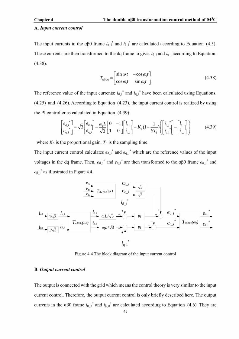
Chapter 4 The double αβ0 transformation control method of M3C
45
A. Input current control
The input currents in the αβ0 frame iα_i* and iβ_i
* are calculated according to Equation (4.5).
These currents are then transformed to the dq frame to give: id_i and iq_i according to Equation.
(4.38).
i i
αβ/dq
i i
sin cos
cos sin
t tT
t t
− =
(4.38)
The reference value of the input currents: id_i* and iq_i
* have been calculated using Equations.
(4.25) and (4.26). According to Equation (4.23), the input current control is realized by using
the PI controller as calculated in Equation (4.39):
* *d_i d_i d_id_i d_ii
6* *q_i q_i q_iq_i q_i6
0 1 13 (1 )
1 03
e i ie iLK
e i ie iST
− = − − + −
(4.39)
where K6 is the proportional gain. T6 is the sampling time.
The input current control calculates ed_i* and eq_i
* which are the reference values of the input
voltages in the dq frame. Then, ed_i* and eq_i
* are then transformed to the αβ0 frame eα_i* and
eβ_i* as illustrated in Figure 4.4.
Tabc/dq(ωi)
+_
+
_
PI
PI
Tdq/αβ0(ωi)
_
_+
+
3
3
eA
eB
eC
ed_i
eq_i
iα_i
iβ_i
Tαβ0/dq(ωi)
id_i
iq_i
id_i*
iq_i*
ed_i*
eq_i*
eα_i*
eβ_i*
iα0
iβ0
1/ 3
1/ 3
i / 3L
i / 3L
Figure 4.4 The block diagram of the input current control
B. Output current control
The output is connected with the grid which means the control theory is very similar to the input
current control. Therefore, the output current control is only briefly described here. The output
currents in the αβ0 frame iα_o* and iβ_o
* are calculated according to Equation (4.6). They are

Chapter 4 The double αβ0 transformation control method of M3C
46
then transformed to the dq frame giving: id_o and iq_o. Next the reference values of the output
currents: id_o* and iq_o
* can be calculated and then using Equation (4.8), the reference value of
the output voltage in the dq frame: ed_o* and eq_o
* are determined. Finally ed_i* and eq_i
* are
transformed to the αβ0 frame eα_o* and eβ_o
* as illustrated in Figure 4.5.
eα_o*
eβ_o*
iα_o
iβ_o
i0α
i0β
Output Current
Control1/ 3
1/ 3Tdq/αβ0(ωi)
ed_o*
eq_o*
Figure 4.5 The block diagram of the output current control
C. Circulating current control
The calculation for the circulating current is specified in Equation (4.5). The reference value
of the circulating current is then calculated by using the P controller as given in Equation (4.40):
* * * *αα βααα βα αα βα
6* * * *αβ ββαβ ββ αβ ββ
i iu u i iK
i iu u i i
= − −
(4.40)
The reference value of four circulating currents: iαα*, iβα
*, iαβ*, iββ
* are determined from Equation
(4.37). As shown in Figure 4.6, the four corresponding reference values of the voltage
components: uαα*, uβα
*, uαβ*, uββ
* in terms of iαα*, iβα
*, iαβ*, iββ
* are subsequently calculated using
Equation (4.40). The eight reference values of the voltage components in the αβ0 frame: eα_i*,
eβ_i*; eα_o
*, eβ_o*; uαα
*, uβα*, uαβ
*, uββ* are then calculated and transformed to the abc frame as
shown in Figure 4.1. Then, the reference values of the nine arm voltages: uxy* are calculated
and by using the modulation technique, PWM signals are generated and send to each SM. The
modulation technique is not discussed in this thesis for the ‘double αβ0 transformation method’.
-k6
+
_
iαα*
iαβiαα iβα iββ
+
_
iβα*
uαβ*
uαα*
uβα*
uββ*
+
_
iαβ*
+iββ
*
_
Figure 4.6 The block diagram of the circulating current control

Chapter 4 The double αβ0 transformation control method of M3C
47
4.3 Illustrative simulation results under output voltage step change operation
The simulation model of M3C using the ‘double αβ0 transformation method’ is developed using
the MATLAB/SIMULINK software. The input side of M3C is connected to the offshore wind
farm (16.7 Hz) while the output side is connected with the Grid (50 Hz). The simulation
parameters is shown in Table 4.1.
Table 4.1 Simulation parameters of the proposed control method
Description Parameters Value
Rated active power P 20 kW
Input RMS line voltage Ei 380 V
Input frequency fi 16.7 Hz
Output RMS line voltage Eo 380 V
Output frequency fo 50 Hz
Arm inductance L 4 mH
Switching frequency fs 4 kHz
Grid-connected filter inductance Lg 1 mH
Grid-connected filter capacitance Cg 10 μF
Capacitance of SM’s capacitor Cxyz 1 mF
Rated dc capacitor voltage UCxyz* 250 V
Number of SMs per arm n 3
4.3.1 Case I: Steady state operation
Figure 4.7 shows the simulation results of M3C under the steady state operation. The input
voltage and input current is in phase which shows the unity power operation. The arm current
as shown in Figure 4.7(c) contains two frequency components: 50 Hz and 16.7 Hz. The three
capacitor voltages of armAa are illustrated in Figure 4.7(e) which equalled with each other and
controlled around 250 V with ±8% voltage ripple. The sum of all capacitor voltages in armAa,
armBa and armCa in sub-converter a is illustrated in Figure 4.7(f) which proves that the energy

Chapter 4 The double αβ0 transformation control method of M3C
48
difference between these three arms is well balanced.
-500
0
500(a) Input Voltage [V]
-50
0
50(b) Input Current [A]
-50
0
50(c) Arm Current [A]
-50
0
50(d) Output Current [A]
200
250
300(e) Capacitor Voltages [V]
0 0.1 0.2 0.3 0.4 0.5
Time [s]
600
750
1000(f) Sum of Capacitor Voltages [V]
eA
eB
eC
iA
iB
iC
iAa
iBaiCa
ia
ibic
uCAaz
uCBa
uCCa
uCAa
Figure 4.7 Simulation results under the steady-state operation
4.3.2 Case II: Dynamic output power operation
In order to verify the control effect of the ‘double αβ0 transformation’ control method, M3C is
tested under dynamic output power (from 20 kW to 24 kW) operation. As shown in Figure 4.8,
the three capacitor voltages of armAa are illustrated in Figure 4.8(d) drops at first and then are
all tightly balanced around 750 V with ±6.7% voltage ripple. This is because the output power
rises instantaneously and the energy within the capacitors are absorbed. However, the capacitors
need to be re-supplied by the energy balancing control so the input current will increase
immediately. When the input power and output power are equalled with each other, the system
has reached a new steady-state operation point. It can be seen that the transition is smooth, the
overshoot is small, and the dynamic performance is good.

Chapter 4 The double αβ0 transformation control method of M3C
49
0
2
410
4 (a) Active and Reactive Power [W]/[Var]
-100
0
100(b) Input Current [A]
-50
0
50(c) Arm Current [A]
-100
0
100(d) Output Current [A]
200
250
300(e) Capacitor Voltages [V]
0 0.1 0.2 0.3 0.4 0.5 0.6 0.7 0.8 0.9 1
Time [s]
600
700
800
900(f) Sum of Capacitor Voltages [V]
P
Q
iA
iB
iC
iAa
iBaiCa
ia
ibic
uCAaz
uCBa
uCCa
uCAa
Figure 4.8 Simulation results under a dynamic output power operation
4.4 Summary
The most commonly used control method of M3C is studied and presented in this chapter. The
analysis and control algorithm needs multiple αβ0 transformations. It decoupled the input,
output and circulating current and calculate the mathematical relationship between the arm
power and capacitor voltage on the αβ0 frame. Determined by the mathematical relationship,
four circulating current components with either input or output frequency are designed to
balance the capacitor voltage. However, the control logic of using the circulating current
components on the αβ0 frame to balance the capacitor voltage is too complex and not clear.
Therefore, it is essential to design a simplified control method for M3C which is discussed in
following chapters.

Chapter 5 Hierarchical Energy Balance Control Method for M3C based on Injecting Output Frequency Circulating Currents
50
Chapter 5 Hierarchical Energy Balance Control Method for M3C based on
Injecting Output Frequency Circulating Currents
The target of this thesis is to develop a simplified control method of M3C for the LFAC
transmission system. Two different control methods have been developed in this thesis and they
are presented in chapter 5 and chapter 6 respectively. In this chapter, the simplified energy
balance control method of M3C with injecting single frequency is discussed in details.
5.1 The mathematical model of sub-converter a
As illustrated in Figure 5.1, M3C is divided into three identical sub-converters. For simplicity
and owing to the symmetry properties, only sub-converter a is considered for deriving the
mathematical model in this section. However, this can be equally applied to the other sub-
converters of M3C.
SM1
ea eb ec
iA
iB
iC
ia ib ic
Sub-converter a Sub-converter b Sub-converter c
iAa iBa iCa iAb iBb iCb iAc iBc iCc
uAa
uBa
uCa
uAb
uBb
uCb
uAc
uBc
uCc
eA
eB
eC
Li
Li
Li
Lo
L L L L L L L L
Lo Lo
L
SMn
SM1
SMn
SM1
SMn
SM1
SMn
SM1
SMn
SM1
SMn
SM1
SMn
SM1
SMn
SM1
SMn
+
−uCxy1
+
−uCxy2
+
−uCxyn
L
ixy
uxy
Structure of each arm
uxy1
+
−
uxy2
+
−
uxyn
+
−
N
O
Figure 5.1 The circuit diagram of Modular Multilevel Matrix Converter
As injecting the output frequency circulating current, each arm current contains three current
components: input current component, output current component and circulating current
component. For better presentation and discussion in the following sections, the input is

Chapter 5 Hierarchical Energy Balance Control Method for M3C based on Injecting Output Frequency Circulating Currents
51
represented by abbreviated letter: i and the output is represented by abbreviated letter: o, while
the circulating current is represented by: cir. Therefore, the arm current in sub-converter a is
given by (1) as follows:
Aa Aa_oAa_i Aa_cir
Ba Ba_oBa_i Ca_cir
Ca Ca_oCa_i Ca_cir
i i i i
i i i i
i i i i
= + +
= + +
= + +
(5.1)
where, iAa_i, iBa_i and iCa_i are the input current components and iAa_o, iBa_o and iCa_o are the
output current components while iAa_cir, iBa_cir and iCa_cir are circulating currents.
It is worth noting that the circulating current flows within the sub-converter and does not
contribute to the input and output currents and the sum of the three circulating currents equals
to zero.
Aa_cir Ba_cir Ca _cir 0i i i+ + = (5.2)
Due to the symmetry property of the proposed M3C, the input current components and the
output current components are one third of the input and output currents, respectively. Therefore,
(5.1) can be further represented by (5.4) as follows:
aAAa _ cir
aBBa_cir
C aCa_cir
Aa
Ba
Ca
3 3
3 3
3 3
iii
iii
i ii
i
i
i
+
+
+
= +
= +
= +
(5.3)
Hence, the arm voltage of sub-converter a can be calculated as:
( ) ( )
( ) ( )
( ) ( )
Aa_i Aa_o Aa_cir
Aa A i o a
Ba_i Aa_o Ba_cir
Ba B i o a
Ca_i Aa_o Ca_cir
Ca C i o a
3 + 3 +
3 + 3 +
3 + 3 +
di di diu e L L L L L e
dt dt dt
di di diu e L L L L L e
dt dt dt
di di diu e L L L L L e
dt dt dt
= − − − −
= − − − −
= − − − −
(5.4)
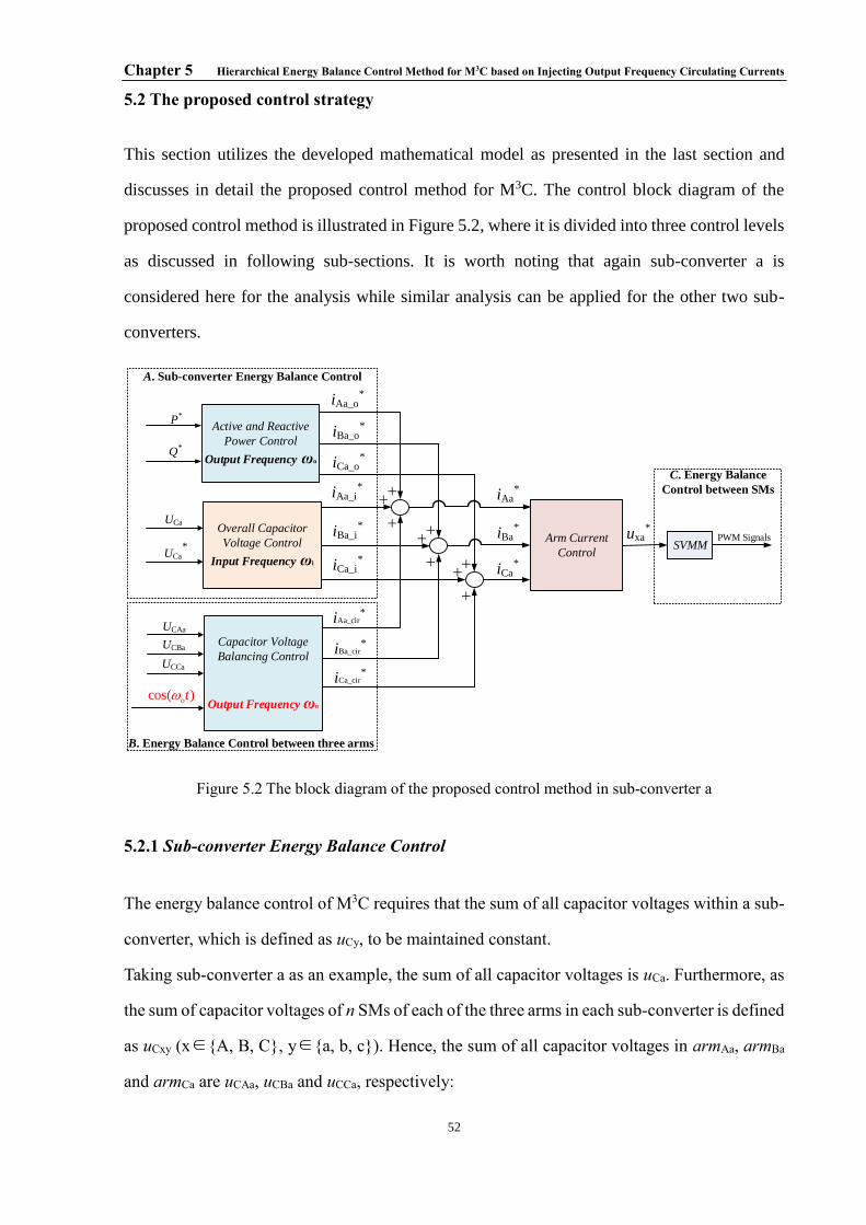
Chapter 5 Hierarchical Energy Balance Control Method for M3C based on Injecting Output Frequency Circulating Currents
52
5.2 The proposed control strategy
This section utilizes the developed mathematical model as presented in the last section and
discusses in detail the proposed control method for M3C. The control block diagram of the
proposed control method is illustrated in Figure 5.2, where it is divided into three control levels
as discussed in following sub-sections. It is worth noting that again sub-converter a is
considered here for the analysis while similar analysis can be applied for the other two sub-
converters.
P*
Q*
Active and Reactive
Power Control
Output Frequency ωo
UCa
UCa*
UCAa
UCBa
UCCa
iAa_cir*
iAa_o*
iBa_i*
A. Sub-converter Energy Balance Control
B. Energy Balance Control between three arms
C. Energy Balance
Control between SMs
Capacitor Voltage
Balancing Control
Output Frequency ωo
Overall Capacitor
Voltage Control
Input Frequency ωi
iBa_o*
iCa_o*
iAa_i*
iCa_i*
++
+++
+++
+
iAa*
iBa*
iBa_cir*
iCa_cir*
SVMMPWM Signals
iCa*
Arm Current
Control
uxa*
ocos( )t
Figure 5.2 The block diagram of the proposed control method in sub-converter a
5.2.1 Sub-converter Energy Balance Control
The energy balance control of M3C requires that the sum of all capacitor voltages within a sub-
converter, which is defined as uCy, to be maintained constant.
Taking sub-converter a as an example, the sum of all capacitor voltages is uCa. Furthermore, as
the sum of capacitor voltages of n SMs of each of the three arms in each sub-converter is defined
as uCxy (x∈{A, B, C}, y∈{a, b, c}). Hence, the sum of all capacitor voltages in armAa, armBa
and armCa are uCAa, uCBa and uCCa, respectively:

Chapter 5 Hierarchical Energy Balance Control Method for M3C based on Injecting Output Frequency Circulating Currents
53
a Aa Ba Ca=C C C Cu u u u+ + (5.5)
where, uCAa, uCBa and uCCa are calculated by (5.6):
CAa CAa1 CAa2 CAan
CBa CBa1 CBa2 CBan
Ca CCa1 CCa2 CCan
C
u u u u
u u u u
u u u u
= + ++
= + ++ = + ++
(5.6)
The arm current consists of input and output current components as given by (5.3), where any
changes in these currents will influence the uCa and vice versa. Hence controlling uCa is the key
to achieve the required energy balance.
a. Active and Reactive Power Control
In Figure 5.3, P* and Q* are reference values of the required active and reactive power,
respectively, which are dependent on the demand from the output side.
P*
Q*
id_o*
iq_o*
Active and
Reactive Power
Control1/3
ixa_o*
ixb_o*
ixc_o*
ia*
ib*
ic*
Tdq/abc(ωo)
Figure 5.3 Active and reactive power control block diagram
The output voltages are transferred to dq frame (i.e. ed and eq) using (5.7):
abcdq
cos cos cos2
3sin sin sin
2 2
3 3
2 2
3 3
T
− +
=
− − − − +
(5.7)
Then the reference values, id_o* and iq_o* of the output currents, can be obtained from (5.8):
d d
q d
* *_ o
* *_ o
P e i
Q i e
=
= −
(5.8)
Therefore, the reference values of the output currents ia*, ib* and ic* can then be calculated by
transforming id_o* and iq_o* back to abc frame using (5.9).

Chapter 5 Hierarchical Energy Balance Control Method for M3C based on Injecting Output Frequency Circulating Currents
54
dqabc
2
3
cos sin
2 2cos( ) sin( )
3 3
2 2cos( ) sin( )
3 3
T
=
− − −
+ − +
(5.9)
With reference to (5.3), in each sub-converter the output current components within the arm
current is equal to one third of the output current. Therefore, the reference value of output
current components ixa_o*, ixb_o* and ixc_o
* of the nine arms currents of three sub-converters in
M3C have been calculated as shown in Figure 5.3.
where:
*
y*
xy_o =3
ii (5.10)
b. Overall capacitor voltage control
In Figure 5.4, the low pass filter functions as filtering out the ac fluctuation of uCa. After passing
through the filter, the DC capacitor voltage of uCa is defined as UCa. UCa* is the reference value
of UCa. When UCa is bigger than UCa* it means there is an extra energy that is stored within the
sub-converter a. Conversely, when UCa is smaller than UCa*, it means the energy provided to
the sub-converter a is insufficient. Therefore, the input side must increase the energy provided
to sub-converter a. The ultimate goal of this control block is to keep UCa equal to UCa* which
means the input side meets the required energy demand.
iq_i*=0
Tdq/abc(ωi)PI
id_i*
+−
uCa
iAa_i*
iBa_i*
iCa_i*
UCa
UCa*
Figure 5.4 The block diagram of the overall capacitor voltage control
In Figure 5.4, id_i* and iq_i* are reference values of the direct and quadrature axis components
of the input current components iAa_i, iBa_i and iCa_i, respectively. Furthermore, iq_i* is set to zero

Chapter 5 Hierarchical Energy Balance Control Method for M3C based on Injecting Output Frequency Circulating Currents
55
to achieve a unity power factor. Therefore, the reference values of the input current components:
iAa_i*, iBa_i* and iCa_i
* in Figure 5.4 have been calculated according to transformation matrix
(5.9).
It is important to mention that the amplitude of three arm currents iAa_i, iAb_i, iAc_i in sub-
converters a, b, c, respectively are not necessary equalled with each other. When there is an
unbalanced condition at the gird, the proposed control method is able to self-balance the energy
between sub-converters.
5.2.2 Energy Balance Control between the three arms of the sub-converter (Capacitor voltage
balancing control)
Although the overall energy of the sub-converter is controlled, however it is not necessarily
means that the energy between the three arms of the sub-converter is balanced. Therefore,
another control level is required, which utilizes the circulating current. With the circulating
current control, the arm with bigger energy compensates the arm with smaller energy, to realize
the dynamic energy balance within each sub-converter.
Figure 5.5 illustrates the proposed circulating current control, which equally balances the
energy across the three arms of the sub-converter. The sum of all capacitor voltages in armAa,
armBa and armCa are uCAa, uCBa and uCCa, respectively. The low pass filter functions as filtering
out the ac fluctuation of uCAa, uCBa and uCCa. After passing through the filter, these three DC
capacitor voltages are defined as UCAa, UCBa and UCCa. Then, these three values are averaged as
in (5.11):
Ca CAa CBa CCa( ) / 3U U U U= + + (5.11)

Chapter 5 Hierarchical Energy Balance Control Method for M3C based on Injecting Output Frequency Circulating Currents
56
+−
PIiAa_cir
+−
PIiBa_cir
++
+
1/3
IAa_cir
IBa_cir
uCAa
uCBa
uCCa
UCAa
UCBa
UCCa
UCAa
UCBaUCa
iCa_cir
+
iAa_cir
iBa_cir +-1
( )ocos t
( )ocos t
Figure 5.5 The block diagram of the capacitor voltage balancing control in sub-converter a
After UCAa and UCBa are compared with the mean value and the error is processed the PI
controller, the RMS value of the circulating currents: IAa_cir*, IBa_cir
* are then calculated as
portrayed in Figure 5.5.
In order to realize the independent control of each sub-converter, the phase angle: ωot of output
voltage ea is set as the reference phase angle for these three circulating currents since these three
arms of sub-converter is connected with output phase a. Therefore, the calculation of the
circulating currents is shown in (5.12):
* *
Aa_cir Aa_cir o
* *
Ba_cir Ba_cir o
* * *
Ca_cir Aa_cir Ba_cir
cos( )
cos( )
i I t
i I t
i i i
=
= = − −
(5.12)
The energy difference between three arms of sub-converter a is caused by the active power that
are generated by circulating currents, these three active power’s value are defined by: PAa_cir,
PBa_cir and PCa_cir which can be calculated as follows:
*
Aa_cir a
Aa _ cir
*
Ba_cir a
Ba _ cir
*
Ca_cir a
Ca _ cir
2
2
2
I EP
I EP
I EP
=
=
=
(5.13)
Figure 5.6 shows one possible power exchange path between the three arms in sub-converter a,
which is further discussed in details in the remaining of this section.
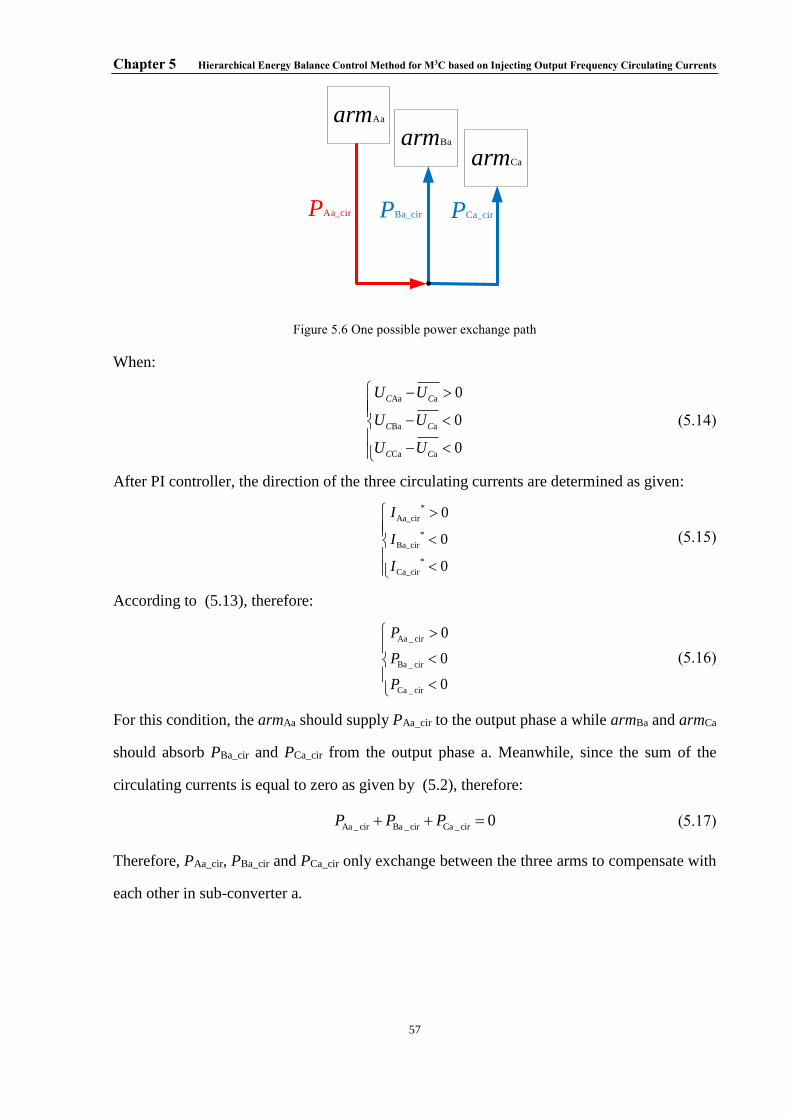
Chapter 5 Hierarchical Energy Balance Control Method for M3C based on Injecting Output Frequency Circulating Currents
57
armAa
armCa
armBa
PAa_cir PBa_cir PCa_cir
Figure 5.6 One possible power exchange path
When:
Aa a
Ba a
Ca a
0
0
0
C C
C C
C C
U U
U U
U U
−
−
−
(5.14)
After PI controller, the direction of the three circulating currents are determined as given:
*
Aa_cir
*
Ba_cir
*
Ca_cir
0
0
0
I
I
I
(5.15)
According to (5.13), therefore:
Aa _ cir
Ba _ cir
Ca _ cir
0
0
0
P
P
P
(5.16)
For this condition, the armAa should supply PAa_cir to the output phase a while armBa and armCa
should absorb PBa_cir and PCa_cir from the output phase a. Meanwhile, since the sum of the
circulating currents is equal to zero as given by (5.2), therefore:
Aa _cir Ba _cir Ca _cir 0P P P+ + = (5.17)
Therefore, PAa_cir, PBa_cir and PCa_cir only exchange between the three arms to compensate with
each other in sub-converter a.

Chapter 5 Hierarchical Energy Balance Control Method for M3C based on Injecting Output Frequency Circulating Currents
58
5.2.3 The arm current Control
Figure 5.7 shows the arm current control according to (5.3) in sub-converter a. The reference
value of the arm current ixa* consists of three current components: ixa_i
*, ixa_o* and ixa_cir that have
been calculated in the previous sections.
+PI
+
−
+−
SVMM
ixa_cir
+
+
ixa
−
eA
ea
uxa*
ixa*
PWM Signals
ixa_o*
ixa_i*
Figure 5.7 Arm current control block diagram
The difference between the ixa and ixa* are calculated at first, after which the PI controller along
with a feedforward term as per (5.4) is used to calculate the reference value of three arm
voltages (noted by uxa*). Then, the selective voltage mapping modulation technique (SVMM),
as discussed in the following section, is designed to generate the PWM signals of each SM.
5.2.4 Energy balance control between n SMs of each arm (Selective Voltage Mapping
Modulation)
In each arm, each SM’s energy should be balanced which indicates the balance of the capacitor
voltage. Therefore, a third control level is required to control the SM’s capacitors voltage. The
selective voltage mapping modulation (SVMM) is designed based on the phase disposition
modulation method (PDPWM) but the sorting algorithm is specifically designed for M3C. The
voltages of all SM’s capacitors are being measured and sorted according to their values. Then
based on the arm current’s direction these capacitors are mapped according to the sorting
algorithm to realize the goal of balancing energy between the n SMs. The details of the control
strategy is further explained below.

Chapter 5 Hierarchical Energy Balance Control Method for M3C based on Injecting Output Frequency Circulating Currents
59
+
−
+
−
uCxaz
ixa
iCxaz(t) S3NOT
SCxaz1
S1
S2NOT S4
uxaz
PWM1
PWM6
PWM10
SCxaz2
......
t0
1
-1
Am
pli
tud
e [
p.u
.]
(a) (b)
Figure 5.8 (a) Full bridge SM (b) PWM signals of five SMs
The instantaneous power of each SM is defined as: pCxyz. The dc capacitor voltage of the SM is
defined as: UCxyz as discussed in the previous section. The reference value of the dc capacitor
voltage is defined as: UCxyz*. Each SM needs two switching signals which can be presented as
SCxaz1, SCxaz2 in sub-converter a as shown in Figure 5.8(a). Assuming there are five SMs in armAa
of sub-converter a, then two switching signals are SCAaz1, SCAaz2. Therefore, the output voltage
of the SM in armAa is determined from:
Aaz CAaz1 Aa CAaz2 Aa(1 )C z C zu S u S u= − − (5.18)
Whereas, the instantaneous power of each SM is calculated as:
Aaz Aaz Aa CAaz1 CAaz2 Aa Aa( 1) C zp u i S S u i= = + − (5.19)
Hence:
CAa1 Aa1 Aa CAa11 CAa12 Aa1 Aa
CAa2 Aa2 Aa CAa21 CAa22 Aa2 Aa
CAa5 Aa5 Aa CAa51 CAa52 Aa5 Aa
( 1)
( 1)
( 1)
C
C
C
p u i S S u i
p u i S S u i
p u i S S u i
= = + −
= = + − = = + −
(5.20)
In Figure 5.8(b), the reference value of arm voltage: uAa* is the reference signal and there are
ten carrier signals in terms of five SMs. It generates ten PWM signals that defined as: PWM1,
PWM2 … PWM10. For example, when iAa>0, each SM’s instantaneous power could be sorted
descending in (5.21):

Chapter 5 Hierarchical Energy Balance Control Method for M3C based on Injecting Output Frequency Circulating Currents
60
* *
5 10 Aa 4 9 Aa
* *
4 9 Aa 3 8 Aa
* *
3 8 Aa 2 7 Aa
* *
2 7 Aa 1 6 Aa
( 1) ( 1)
( 1) ( 1)
( 1) ( 1)
( 1) ( 1)
Cxyz Cxyz
Cxyz Cxyz
Cxyz Cxyz
Cxyz Cxyz
PWM PWM u i PWM PWM u i
PWM PWM u i PWM PWM u i
PWM PWM u i PWM PWM u i
PWM PWM u i PWM PWM u i
+ − + −
+ − + −
+ − + −
+ − + −
(5.21)
Then the capacitor voltages should be sorted ascending in order to balance the energy between
five SMs in armAa. Assuming uCAa1<uCAa2<uCAa3<uCAa4<uCAa5, then PWM signals should be
mapped to the certain switching signals of each SM as shown in Figure 5.9, which enables the
balancing of the capacitors voltage within each arm.
PWM5
PWM10
SCAa11
SM One
SCAa12
PWM4
PWM9
SCAa21
SM Two
SCAa22
PWM3
PWM8
SCAa31
SM Three
SCAa32
PWM2
PWM7
SCAa41
SM Four
SCAa42
PWM1
PWM6
SCAa51
SM Five
SCAa52
Figure 5.9 PWM signals mapping of SVMM
5.3 Illustrative Simulation Results
The simulation model of M3C for LFAC is developed using MATLAB/SIMULINK software.
The input side of M3C is connected to the offshore wind farm (16.7 Hz) while the output side
is connected with the on-shore power grid (50 Hz). The simulation parameters are shown in
Table II. The offshore wind farm can be up to 630 MW (i.e. The London Array Offshore wind
farm). However, on the other hand, 10 MW windfarms are also available in some other areas,
such as: offshore wind farm in Taiwan (8 MW), Spain (5 MW), Norway (2 MW) and France (2
MW) [97]. Nevertheless, the simulation model is aimed at verifying the effectiveness of the
developed voltage balance control method proposed in this paper and it can easily extend to

Chapter 5 Hierarchical Energy Balance Control Method for M3C based on Injecting Output Frequency Circulating Currents
61
higher rated systems with different simulation parameters. There are five capacitors in each arm.
The standard 6.6 kV 1.5 kA IGBT module such as the product from Infineon is considered as
the power switch to build the SM. The proposed system is tested under different operating
conditions to validate the performance of the proposed control strategy.
Table Ⅱ
Simulation parameters
Description Parameters Value
Rated Active Power P 10 MW
Input RMS line voltage Ei 11 kV
Input frequency fi 16.7 Hz
Input inductance Li 4 mH (3.4%)
Output RMS line voltage Eo 11 kV
Output frequency fo 50 Hz
Output inductance Lo 4 mH (3.4%)
Arm inductance L 5 mH (4.3%)
Capacitance of SM’s capacitor Cxyz 5.1 mF
Rated dc capacitor voltage UCxyz* 5 kV
Number of SMs per arm n 5
Switching frequency fs 5 kHz
5.3.1 Case I: Steady-state operation
Figure 5.10 shows the simulation results under steady-state operation, where Figure 5.10 (a)
and (b) are the input voltage and input current with no phase shift, demonstrating the unity
power operation. The arm current contains two frequency components as illustrated in Figure
5.10 (c). According to [95], the tolerance of the capacitor voltage ripple should be ±10%. In
Figure 5.10 (e), the capacitor voltages of armAa in sub-converter a is illustrated, where all five
capacitor voltages are tightly balanced around 5 KV with ±2.5% voltage ripple. Furthermore,
Figure 5.10 (f) shows the sum of capacitor voltages of all SMs in sub-converter a, which are

Chapter 5 Hierarchical Energy Balance Control Method for M3C based on Injecting Output Frequency Circulating Currents
62
perfectly controlled around 25kV.
-1
0
110
4 (a) Input Voltage [V]
-1000
0
1000(b) Input Current [A]
-500
0
500(c) Arm Current [A]
-1000
0
1000(d) Output Current [A]
4950
5000
5050(e) Capacitor Voltages [V]
0 0.1 0.2 0.3 0.4 0.5
Time [s]
2.48
2.5
2.5210
4 (f) Sum of Capacitor Voltages [V]
eAeBeC
iAiB
iC
iAaiBa
iCa
iaib
ic
uCAaz
uCAa
uCBa
uCCa
Figure 5.10 Simulation results under steady-state operation
5.3.2 Case II: Dynamic output power operation
Figure 5.11 shows the simulation results under dynamic output power operation. Specifically,
Figure 5.11(a) demonstrates the case when the active power supplied by the input side increases
from 10 MW to 11 MW at 0.5 s, where the reactive power maintain as zero for the unity power
operation. It is worth noting that the capacitor voltages in Figure 5.11(e) and (f) slightly
decreased to compensate the active power to the gird from 0.5 s and the proposed control
strategy successfully managed to maintain the voltage balance at 0.8 s.

Chapter 5 Hierarchical Energy Balance Control Method for M3C based on Injecting Output Frequency Circulating Currents
63
0
5
10
1510
6 (a) Active and Reactive Power [W]/[Var]
-1000
0
1000(b) Input Current [A]
-500
0
500(c) Arm Current [A]
-1000
0
1000(d) Output Current [A]
4900
5000
5100(e) Capacitor Voltages [V]
0 0.5 1 2
Time [s]
2.45
2.5
2.5510
4 (f) Sum of Capacitor Voltages [V]
P
Q
iAiB
iC
iAaiBa
iCa
iaib
ic
uCAaz
uCAa
uCBa
uCCa
Figure 5.11 Simulation results under a dynamic output power operation
5.3.3 Case III: Unbalanced grid voltage condition
The 5% negative sequence component has been added in the input side of M3C which cause the
unbalanced grid voltage condition as shown in Figure 5.12(a), the proposed control strategy
illustrated the good performance under this condition. From 0.5 s to 0.8 s, the capacitor voltage
balancing control has been deactivated to illustrate the effect of the circulating current. As it
can be noticed, from 0 s to 0.5 s, the circulating current control is deactivated, which causing
the five capacitors voltages in armAa in sub-converter a deviating (i.e. gradually increasing)
from the reference voltage. This has also influenced the sum of capacitor voltages of armAa
(increasing) and armBa, armCa (decreasing) as shown in Figure 5.12. On the other hand, the

Chapter 5 Hierarchical Energy Balance Control Method for M3C based on Injecting Output Frequency Circulating Currents
64
effect of the circulating current can be obviously observed when it is activated at 0.8 s, where
the capacitor voltages are quickly re-balanced around 5 kV.
-1
0
110
4 (a) Input Voltage [V]
-1000
0
1000(b) Input Current [A]
-500
0
500(c) Arm Current [A]
-1000
0
1000(d) Output Current [A]
4800
5000
5200(e) Capacitor Voltages [V]
0 0.5 1 1.5
Time [s]
2.4
2.5
2.610
4 (f) Sum of Capacitor Voltages [V]
Deactivated
eAeBeC
iAiB
iC
iAaiBa
iCa
iaib
ic
uCAaz
uCAa
uCBa
uCCa
Figure 5.12 Simulation results under unbalanced grid voltage condition
5.4 Summary
Obviously, the proposed control method does not need multiple αβ0 transformations to
decouple the input, output and circulating current. Furthermore, in the ‘double αβ0
transformation’ control method, four circulating currents on the αβ0 frame are designed to
balance the capacitor voltage between nine arms. Both characteristics of the ‘double αβ0
transformation’ control method brings the disadvantages of increasing the complexity of the
control algorithm. However, the proposed control method achieved the fully independent

Chapter 5 Hierarchical Energy Balance Control Method for M3C based on Injecting Output Frequency Circulating Currents
65
control of each sub-converter. The injection of output frequency circulating current has been
designed easily and accurately for the purpose of compensating the energy difference between
the three arms of each sub-converter, which dramatically decrease the mathematical calculation
and control complexity. Furthermore, the selective voltage mapping modulation technique is
designed that balances the energy between n sub-modules within each arm. The experimental
results from a scaled down laboratory prototype proved the performance of the proposed control
method under steady-state and different dynamic operating conditions. The experimental results
from a scaled down laboratory prototype which is presented in chapter 7, is in a perfect match
with the simulation ones.

Chapter 6 Hierarchical Energy Balance Control Method for M3C based on Injecting Two Frequency Circulating Currents
66
Chapter 6 Hierarchical Energy Balance Control Method for M3C based on
Injecting Two Frequency Circulating Currents
This chapter presented an improved control method for the energy balance of M3C. It is
achieved by incorporating both input and output frequency circulating current on the basis of
two set of sub-converters.
6.1 Circuit topology of M3C
Figure 6.1 shows the circuit diagram for M3C which is discussed in the previous chapter where
three sub-converters are defined as sub-converter a, sub-converter b and sub-converter c as
illustrated in Figure 6.1. In this chapter, the proposed control method for M3C is based on
dividing the converter into six sub-converters instead of three as in the previous chapter. Apart
from sub-converters a, b and c, the other three sub-converters of M3C are shown in Figure 6.2
which are named as sub-converter A, sub-converter B and sub-converter C.
SM1
ea eb ec
iA
iB
iC
ia ib ic
Sub-converter a Sub-converter b Sub-converter c
iAa iBa iCa iAb iBb iCb iAc iBc iCc
uAa
uBa
uCa
uAb
uBb
uCb
uAc
uBc
uCc
eA
eB
eC
Li
Li
Li
Lo
L L L L L L L L
Lo Lo
L
SMn
SM1
SMn
SM1
SMn
SM1
SMn
SM1
SMn
SM1
SMn
SM1
SMn
SM1
SMn
SM1
SMn
+
−uCxy1
+
−uCxy2
+
−uCxyn
L
ixy
uxy
Structure of each arm
uxy1
+
−
uxy2
+
−
uxyn
+
−
N
O
Figure 6.1 Circuit diagram for M3C divided into sub-converters a, b and c
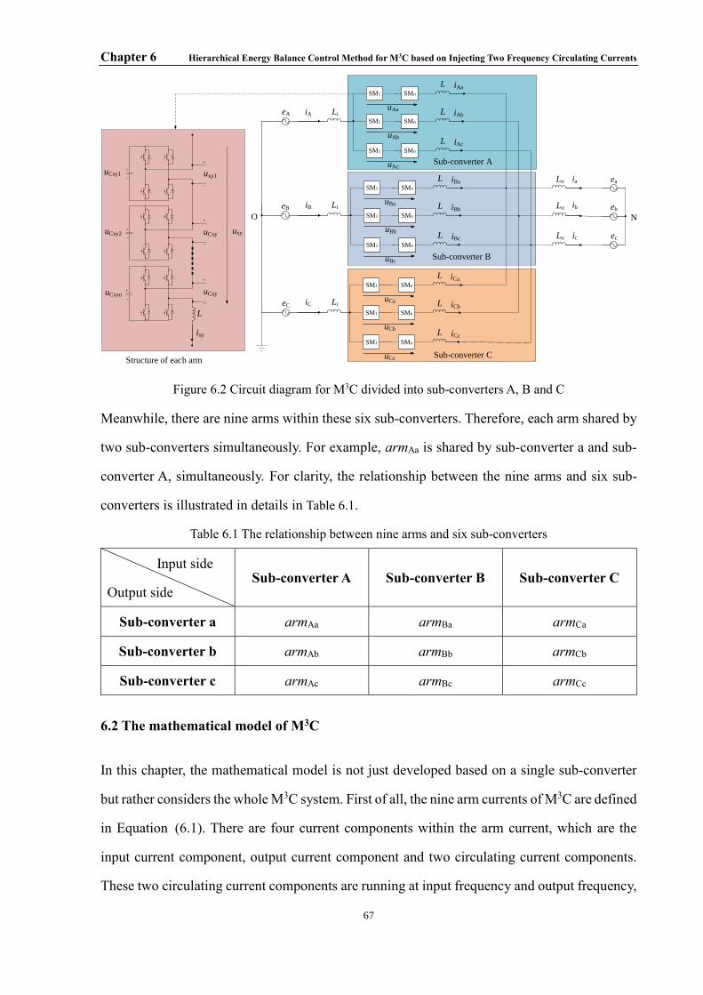
Chapter 6 Hierarchical Energy Balance Control Method for M3C based on Injecting Two Frequency Circulating Currents
67
iA
iB
iC
eA
eB
eC
Li
Li
Li
SM1
iAa
uAa
LSMn
iAbL
iAcL
SM1
uAb
SMn
SM1
uAc
SMn
SM1
iBa
uBa
LSMn
iBbL
iBcL
SM1
uBb
SMn
SM1
uBc
SMn
SM1
iCa
uCa
LSMn
iCbL
iCcL
SM1
uCb
SMn
SM1
uCc
SMn
eaia
Lo
eb
ec
Lo
Lo
ib
ic
Sub-converter A
Sub-converter B
Sub-converter C
+
−uCxy1
+
−uCxy2
+
−uCxyn
L
ixy
uxy
Structure of each arm
uxy1
+
−
uCxy
+
−
uCxy
+
−
NO
Figure 6.2 Circuit diagram for M3C divided into sub-converters A, B and C
Meanwhile, there are nine arms within these six sub-converters. Therefore, each arm shared by
two sub-converters simultaneously. For example, armAa is shared by sub-converter a and sub-
converter A, simultaneously. For clarity, the relationship between the nine arms and six sub-
converters is illustrated in details in Table 6.1.
Table 6.1 The relationship between nine arms and six sub-converters
Input side
Output side Sub-converter A Sub-converter B Sub-converter C
Sub-converter a armAa armBa armCa
Sub-converter b armAb armBb armCb
Sub-converter c armAc armBc armCc
6.2 The mathematical model of M3C
In this chapter, the mathematical model is not just developed based on a single sub-converter
but rather considers the whole M3C system. First of all, the nine arm currents of M3C are defined
in Equation (6.1). There are four current components within the arm current, which are the
input current component, output current component and two circulating current components.
These two circulating current components are running at input frequency and output frequency,

Chapter 6 Hierarchical Energy Balance Control Method for M3C based on Injecting Two Frequency Circulating Currents
68
respectively. The details of the circulating current control will be discussed in this chapter.
Nine arm currents of M3C are given by:
xy xy_oxy_i xy_cir
xy_cir xy_cir_i xy_cir_o
i i i i
i i i
+
= +
= + (6.1)
where ixy_o is the output current component. ixy_cir_i is the circulating current running at input
frequency of the corresponding arm while ixy_cir_o is the circulating current running at output
frequency of the corresponding arm.
Since the three sub-converters a, b and c are connected to the corresponding output phase a, b
and c as shown in Figure 6.1, therefore it is easy to deduce that the sum of the three arm currents
in each sub-converter is equal to the corresponding output phase current. Meanwhile, the sum
of three circulating currents within each sub-converter is equal to zero as discussed in the
previous chapter. Hence, the required calculations of arm currents for sub-converters a, b and c
are given in Equations (6.2)-(6.4).
For sub-converter a:
Aa Ba Ca a
Aa _ cir _ o Ba _ cir _ o Ca _ cir _ o 0
i i i i
i i i
+ + =
+ + = (6.2)
For sub-converter b:
Ab Bb Cb b
Ab _ cir _ o Bb _ cir _ o Cb _ cir _ o 0
i i i i
i i i
+ + =
+ + = (6.3)
For sub-converter c:
Ac Bc Cc c
Ac_ cir _ o Bc_ cir _ o Cc_ cir _ o 0
i i i i
i i i
+ + =
+ + = (6.4)
Similarly, the sub-converters A, B and C are connected to the corresponding input phase A, B
and C as illustrated in Figure 6.2. Therefore, the sum of the three arm currents is equal to the
corresponding input phase current while the sum of the three circulating currents within each
sub-converter is equal to zero. The required calculations of arm currents for sub-converters A,
B and C are given in Equations (6.5)-(6.7).
For sub-converter A:

Chapter 6 Hierarchical Energy Balance Control Method for M3C based on Injecting Two Frequency Circulating Currents
69
Aa Ab Ac A
Aa _ cir _ i Ab _ cir _ i Ac_ cir _ i 0
i i i i
i i i
+ + =
+ + = (6.5)
For sub-converter B:
Ba Bb Bc B
Ba _ cir _ i Bb _ cir _ i Bc _ cir _ i 0
i i i i
i i i
+ + =
+ + = (6.6)
For sub-converter C:
Ca Cb Cc C
Ca _ cir _ i Cb _ cir _ i Cc_ cir _ i 0
i i i i
i i i
+ + =
+ + = (6.7)
Then, the output voltages for each arm are defined by Equation (6.8) as:
xa_i xa_o xa_cir
xa x i o a
xb_i xb_o xb_cir
xb x i o b
xc_i xc_o xc_cir
xc x i o c
( ) ( )
( ) ( )
( ) ( )
di di diu e L L L L L e
dt dt dt
di di diu e L L L L L e
dt dt dt
di di diu e L L L L L e
dt dt dt
= − + − + − −
= − + − + − −
= − + − + − −
(6.8)
6.3 The Proposed control strategy
The block diagram for the overall energy balance control strategy is shown in Figure 6.3. There
are two main differences in terms of the design of the control strategy. Firstly, the energy
balance control of the whole M3C has been added in Control Level One. Secondly, the energy
balance control between the six sub-converters has been considered in this control strategy. This
is achieved by using the circulating current control (two different frequencies) in Control Level
Two. This control method enables the energy to be balanced between the nine arms of M3C.
The details of the proposed control method are discussed in the following sub-sections.

Chapter 6 Hierarchical Energy Balance Control Method for M3C based on Injecting Two Frequency Circulating Currents
70
P*
Q*
Active and Reactive
Power Control
Output Frequency ωo
uC
uC*
uCAa
uCBa
uCCa
iAa_cir_o*
ixa_o*
iBy_i*
A. Energy Balance Control of the M3C
B. Energy Balance Control between three arms
C. Energy Balance
Control between SMs
Capacitor Voltage
Balancing Control
Output Frequency ωo
Overall Capacitor
Voltage Control
Input Frequency ωi
ixb_o*
ixc_o*
iAy_i*
iCy_i*
iAa*
iBa*
iBa_cir_o*
iCa_cir_o*
SVMMPWM Signals
iCa*
Arm Current
Control
uxa*
uCAa
uCBa
uCCa
iAa_cir_i*
C. Energy Balance Control between sub-converters
Capacitor Voltage
Balancing Control
Input Frequency ωi
iBa_cir_i*
iCa_cir_i*
+
+
+
+
+
+
+ +
+ +
+
+
ocos( )t
icos( )t
Figure 6.3 The block diagram of the proposed control method in sub-converter a and sub-converter A
6.3.1 Energy balance control of M3C
The first control level of the overall energy balance control strategy to balance the energy of
the whole M3C. Therefore, the sum of all the capacitor voltages in M3C should be maintained
constant. The input and output currents have an effect on the sum of capacitor voltages.
Therefore, the key aim is to keep capacitor voltage sum balanced so that the energy is balanced.
The sum of all capacitor voltages in M3C: uC is calculated as:
a b cC C C Cu u u u= + + (6.9)
where uCb, uCc are the sum of all capacitor voltages in sub-converter b and c, respectively.
a. Output current control
The output current control block diagram is shown in Figure 6.4 which is same as the output
current control discussed in chapter 6. Analysing M3C according to Figure 6.1 where the

Chapter 6 Hierarchical Energy Balance Control Method for M3C based on Injecting Two Frequency Circulating Currents
71
converter is divided into sub-converters a, b and c. Therefore, the output current components
within the arm current are equal to one third of the output current in each sub-converter. Thereby,
the reference value of output current components ixa_o*, ixb_o* and ixc_o
* of the nine arm currents
in M3C have been calculated as:
*
y*
xy _ o3
ii = (6.10)
P*
Q*
id_o*
iq_o*
Active and
Reactive Power
Control
1/3
ixa_o*
ixb_o*
ixc_o*
ia*
ib*
ic*
Tdq/abc(ωo)
Figure 6.4 Active and reactive power control block diagram
b. Input current control
The control theory of the input current control is similar to that described in the chapter 5.
However, the control target of the input current control in this chapter is the energy balance of
M3C, where uC* in Figure 6.5 is the reference value for uC. When uC is bigger than uC
*, it means
there is an extra energy stored within M3C, therefore the input side must decrease the energy
that is provided to the converter. Conversely, when uC is smaller than uC*, it means the energy
provided to the converter is insufficient, therefore the input side must increase the energy
provided to M3C. The ultimate goal of this control block is to keep uC equal to uC* which means
the input side meets the required energy demand.
iq_i*=0
Tdq/abc(ωi)PI
id_i*
+−
UC
UC*
iA*
iB*
iC*
1/3
iAy_i*
iBy_i*
iCy_i*
Figure 6.5 The overall capacitor voltage control block diagram

Chapter 6 Hierarchical Energy Balance Control Method for M3C based on Injecting Two Frequency Circulating Currents
72
The reference values of the input current: iA*, iB* and iC
* are shown in Figure 6.5. Analysing
M3C according to Figure 6.2 where the converter is divided into sub-converters A, B and C.
Therefore, the input current components within the arm current are equal to one third of the
input current in each sub-converter. Hence, the reference value of input current components
iAy_i*, iBy_i* and iCy_i
* of the nine arm currents in M3C are calculated from:
** x
xy _ i3
ii = (6.11)
6.3.2 Energy balance control between the three arms in the sub-converter A (circulating
current control)
As M3C is divided into sub-converters A, B and C according to Figure 6.2, therefore the next
control level is the energy balance between the three arms in sub-converters A, B and C. In this
sub-section, only sub-converter A is discussed in details as an example. The energy balance
control between the three arms armAa, armAb and armAc in sub-converter A is realized by
injecting the circulating current with input frequency. Meanwhile, it is important to be noticed
that armAa in sub-converter A which also belongs to sub-converter a as presented in Table 6.1.
Similarly, the other two arms in sub-converter A: armAb belongs to sub-converter b while armAc
belongs to sub-converter c. Therefore, this control level is also the energy balance control
between the sub-converter a, sub-converter b and sub-converter c.
Figure 6.6 shows the energy balance control between the three arms in sub-converter A. The
sum of the capacitor voltages in the three arms: armAa, armAb and armAc are defined as: uCAa,
uCAb and uCAc, respectively. After passing through the low-pass filter, these three values are
denoted by: UCAa, UCab and UCAc. Then the mean value of these three values can be calculated
from:
A Aa Ab Ac( ) / 3C C C CU U U U= + + (6.12)

Chapter 6 Hierarchical Energy Balance Control Method for M3C based on Injecting Two Frequency Circulating Currents
73
+−
PI-IAa_cir_i
+−
PI-IAb_cir_i
++
+
1/3
uCAa
uCAb
uCAc
UCAa
UCAb
UCAc
UCAa
UCAbUCA
iAa_cir_i
iAb_cir_i
iAc_cir_i
-1
-1
+
iAa_cir_i
iBa_cir_i +-1
( )icos t
( )icos t
Figure 6.6 The block diagram of the capacitor voltage balancing control in sub-converter A
After UCAa, UCAb and UCAc are compared with the mean value and the error is processed in the
PI controller, the peak value of the circulating currents: IAa_cir_i, IAb_cir_i and IAc_cir_i are then
calculated as illustrated in Figure 6.6. Then, these three values times the constant: -1 because
of the opposite direction compared with eA. The phase angle: ωit of the input voltage eA is set
as a reference phase angle for these three circulating currents. Thereby, the circulating current
(input frequency) can be calculated as follows:
Aa_cir_i Aa_cir_i i
Ab_cir_i Ab_cir_i i
Ac_cir_i Aa_cir_i Ab_cir_i
cos( )
cos( )
i I t
i I t
i i i
= −
= −
= − −
(6.13)
The value of three active powers that are generated by these three circulating currents are
defined as: PAa_cir, PAb_cir and PAc_cir which are calculated by:
Aa_cir_i A
Aa _ cir_i
Ab_cir_i A
Ab _ cir_i
Ac_cir_i A
Ac _ cir_i
2
2
2
I EP
I EP
I EP
= −
= −
= −
(6.14)
Figure 6.7(a) shows an example of power exchange path between the three arms in sub-
converter A which is also the power exchange path between sub-converter a, b and c as
illustrated in Figure 6.7(b). This example power exchange path is further discussed in details in
the remainder of this section.

Chapter 6 Hierarchical Energy Balance Control Method for M3C based on Injecting Two Frequency Circulating Currents
74
armAa
armAc
armAb
PAa_cir PAb_cir PAc_cir
Sub-converter a Sub-converter cSub-converter b
(a) (b)
...
...
...armAa
armAc
armAb
PAa_cir PAb_cir PAc_cir
Sub-converter A
Figure 6.7 An example power exchange path (a) Sub-converter A (b) Sub-converter a, b and c
When:
Aa A
Ab A
Ac A
0
0
0
C C
C C
C C
U U
U U
U U
−
−
−
(6.15)
Then after the PI controller the direction of the three circulating currents are determined from:
Aa_cir_i
Ab_cir_i
Ac_cir_i
0
0
0
I
I
I
(6.16)
And so according to Equation (6.14):
Aa _ cir_i
Ab _ cir_i
Ac _ cir_i
0
0
0
P
P
P
(6.17)
For this condition, the armAa should absorb PAa_cir from the input phase A while armAa and
armAb should supply PAb_cir and PAc_cir to the input phase A. Meanwhile, since the sum of the
circulating currents is equal to zero as given by Equation (6.5), then:
Aa _cir_i Ab_cir_i Ac_cir_i 0P P P+ + = (6.18)
Therefore, the circulating current controller controls the PAa_cir_i, PAb_cir_i and PAc_cir_i exchange
between the three arms to compensate each other in sub-converter A. Hence:
Aa Ab AcP P P= = (6.19)

Chapter 6 Hierarchical Energy Balance Control Method for M3C based on Injecting Two Frequency Circulating Currents
75
where the value of active powers of these three arms: armAa, armAb, armAc are denoted by:
PAa, PAb and PAc, respectively.
The same control theory is applied to sub-converter B and sub-converter C.
In sub-converter B:
Ba Bb BcP P P= = (6.20)
where the value of active powers of these three arms: armBa, armBb, armBc are denoted by: PBa,
PBb and PBc, respectively.
Similarly, in sub-converter C:
Ca Cb CcP P P= = (6.21)
where the value of active powers of these three arms: armCa, armCb, armCc are denoted by: PCa,
PCb and PCc, respectively.
On the other hand, the value of active powers of sub-converter a, b and c are denoted by: Pa, Pb
and Pc, respectively. Therefore, according to Equations (6.19)-(6.21), it is easy to be deduced
that:
a b cP P P= = (6.22)
where,
a Aa Ba Ca
b Ab Bb Cb
c Ac Bc Cc
P P P P
P P P P
P P P P
= + +
= + + = + +
(6.23)
In summary, the energy balance control between three arms in sub-converter A, B and C,
respectively also ensure balanced the energy between sub-converters a, b and c.
6.3.3 Energy balance control between three arms of the sub-converter a (circulating current
control)
Although the energy of the sub-converters a, b and c is controlled as discussed in the previous
section, however, this does not necessarily mean that the energy between the sub-converters A,
B and C is balanced. Similarly, analysing M3C according to Figure 6.1 where the converter is
divided into sub-converters a, b and c. In this sub-section, only sub-converter a is discussed in

Chapter 6 Hierarchical Energy Balance Control Method for M3C based on Injecting Two Frequency Circulating Currents
76
details for an example. Figure 6.8 illustrates the proposed capacitor voltage balancing control
with injecting circulating current (output frequency), which balances the energy between the
three arms of sub-converter a which is also the energy balance control between sub-converters
A, B and C. The control theory is similar to that discussed in Chapter 5.
+−
PIiAa_cir_o
+−
PIiBa_cir_o
++
+
1/3
IAa_cir_o
IBa_cir_o
uCAa
uCBa
uCCa
UCAa
UCBa
UCCa
UCAa
UCBaUCa
iCa_cir_o
+
iAa_cir_o
iBa_cir_o +-1
( )ocos t
( )ocos t
Figure 6.8 The block diagram of the capacitor voltage balancing control in sub-converter a
The phase angle, ωot of the output voltage ea is set as the reference phase angle for all three
circulating currents since these three arms of sub-converter a are connected with output phase
a. Therefore, the calculation of the circulating currents is given by:
oAa_cir_o Aa_cir_o
oBa_cir_o Ba_cir_o
Ca_cir_o Aa_cir_o Ba_cir_o
cos( )
cos( )
i I t
i I t
i i i
−
=
=
= −
(6.24)
The value of active powers that are generated by the circulating currents are defined as: PAa_cir_o,
PBa_cir_o and PCa_cir_o and are calculated as follows:
Aa_cir_o a
Aa_cir_o
Ba_cir_o a
Ba_cir_o
Ca_cir_0 a
Ca_cir_o
2
2
2
I EP
I EP
I EP
=
=
=
(6.25)
Figure 6.9 shows an example power exchange path between the three arms in sub-converter a,
which is discussed further in details in the remainder of this section.

Chapter 6 Hierarchical Energy Balance Control Method for M3C based on Injecting Two Frequency Circulating Currents
77
armAa
armCa
armBa
pAa_cir
pBa_cir
pCc_cir
Sub-converter A
Sub-converter B
...armAa
armCa
armBa
(a)
pAa_cir pBa_cir pCc_cir
(b)
...
Sub-converter C...
Sub-converter a
Figure 6.9 An example power exchange path (a) Sub-converter a (b) Sub-converter A, B and C
When:
Aa a
Ba a
Ca a
0
0
0
C C
C C
C C
U U
U U
U U
−
−
−
(6.26)
Then after the PI controller, the direction of the three circulating currents are determined from:
Aa_cir_o
Ba_cir_o
Ca_cir_o
0
0
0
I
I
I
(6.27)
And so according to Equation (6.25):
Aa _ cir_o
Ba _ cir_o
Ca _ cir_o
0
0
0
P
P
P
(6.28)
For this condition, the armAa should supply PAa_cir_o to the output phase a while armBa and armCa
should absorb PBa_cir_o and PCa_cir_o from the output phase a. Meanwhile, since the sum of the
circulating currents is equal to zero then:
Aa _cir_o Ba _cir_o Ca _cir_oP P P+ + (6.29)
Therefore, the circulating current controller controls PAa_cir_o, PBa_cir_o and PCa_cir_o only
exchange between the three arms to compensate with each other. Therefore, similar analysis as
discussed in the previous section, it is concluded as:

Chapter 6 Hierarchical Energy Balance Control Method for M3C based on Injecting Two Frequency Circulating Currents
78
Aa Ba Ca
Ab Bb Cb
Ac Bc Cc
P P P
P P P
P P P
= =
= = = =
(6.30)
Hence:
A B CP P P= = (6.31)
where the value of active powers of sub-converter A, B and C are denoted by: PA, PB and PC,
respectively and these three powers are calculated as:
A Aa Ab Ac
B Ba Bb Bc
C Ca Cb Cc
P P P P
P P P P
P P P P
= + +
= + + = + +
(6.32)
In summary, the energy balance control between three arms in sub-converter A, B and C,
respectively also balances the energy between sub-converters a, b and c in the meantime.
According to this sub-section and sub-section 6.3.2, it is important to conclude that:
Aa Ab Ac Ba Bb Bc Ca Cb CcP P P P P P P P P= = = = = = = = (6.33)
Equation (6.33) means that the circulating current control balances the active power of nine
arms in M3C.
6.3.4 The arm current control
Figure 6.10 shows the arm current control of sub-converter a which is developed by Equation
(6.1) The reference value of the arm current ixa* consists of four current components: ixa_i
*, ixa_o*,
ixa_cir_i and ixa_cir_o as described in the previous sections.
+
PI+
−
+−
SVMM
ixa_cir_i +
+
ixa
−
eA
ea
uxa*
ixa*
PWM Signals
ixa_o*
ixa_i*
+
ixa_cir_o
Figure 6.10 Arm current control block diagram

Chapter 6 Hierarchical Energy Balance Control Method for M3C based on Injecting Two Frequency Circulating Currents
79
The difference between the ixa and ixa* are calculated first, then the reference value of the three
arm voltages uxa* can then be calculated by Equation (6.8). By using the selective voltage
mapping modulation technique (SVMM) as discussed in the following section, the PWM
signals can be generated for each SM.
6.3.5 Energy balance control between n SMs of each arm (SVMM)
In each arm, the SM’s energy should be balanced which indicates the balance of the capacitor
voltage. Therefore, a third control level is required to control the SM’s capacitors voltage. The
selective voltage mapping modulation (SVMM) discussed in chapter 6 is considered here again
for this chapter.
6.4 Illustrative simulation results
The simulation model of M3C that function as the frequency converter in the LFAC
transmission system is developed using MATLAB/SIMULINK software which is the same as
discussed in chapter 5. The proposed control method is tested under different operating
conditions to validate the effectiveness and the performance of the control strategy as presented
in this chapter.
6.4.1 Case I: Steady-state operation
Figure 6.11 shows the simulation results under steady-state operation, where Figure 6.11(a) and
(b) are the input voltage and input current respectively with no phase shift, hence demonstrating
the unity power operation. The arm current contains two frequency components as illustrated
in Figure 6.11(c). The capacitor voltages of armAa are illustrated in Figure 6.11(e), where all
five capacitor voltages are tightly balanced around 5 kV with voltage ripple ±5%. Furthermore,
Figure 6.11(f) shows the sum of the capacitor voltages of all SMs in sub-converter a, which are
all perfectly controlled around 25 kV.

Chapter 6 Hierarchical Energy Balance Control Method for M3C based on Injecting Two Frequency Circulating Currents
80
eAeBeC
iAiB
iC
iAaiBa
iCa
iaib
ic
uCAaz
uCAa
uCBa
uCCa
-1
0
110
4 (a) Input Voltage [V]
-1000
0
1000(b) Input Current [A]
(c) Arm Current [A]
-1000
0
1000(d) Output Current [A]
4950
5000
5050(e) Capacitor Voltages [V]
0 0.1 0.2 0.3 0.4 0.5
Time [s]
2.48
2.5
2.5210
4 (f) Sum of Capacitor Voltages [V]
-500
0
500
Figure 6.11 Simulation results under steady-state operation
6.4.2 Case II: Dynamic output power operation
Figure 6.12 shows the simulation results under dynamic output power operation. Specifically,
Figure 6.12(a) demonstrates the case when the active power supplied by the input side increases
from 10 MW to 11 MW at 0.5 s, where the reactive power maintain as zero for the unity power
operation. It is worth noting that the proposed control strategy successfully managed to maintain
the voltage balance of the five SMs’ capacitors in Figure 6.12(e) and (f).

Chapter 6 Hierarchical Energy Balance Control Method for M3C based on Injecting Two Frequency Circulating Currents
81
-1000
0
1000(b) Input Current [A]
-5000
500
(c) Arm Current [A]
-1000
0
1000(d) Output Current [A]
4900
5000
5100(e) Capacitor Voltages [V]
0 0.2 0.4 0.6 0.8 1 1.2 1.4 1.6 1.8 2
Time [s]
2.45
2.5
2.5510
4 (f) Sum of Capacitor Voltages [V]
P
Q
iAiB
iC
iAaiBa
iCa
iaib
ic
uCAaz
uCAa
uCBa
uCCa
0
5
10
1510
6 (a) Active and Reactive Power [W]/[Var]
Figure 6.12 Simulation results under dynamic output power operation
6.5 Comparison between the ‘double αβ0 transformation’ control method and proposed
control methods
In terms of the complexity of the voltage balancing control, the comparison between three
control methods has been given in Figure 6.13. The complexity of the mathematical calculation
is determined by how many accumulator, multiplier, sin and cos in the coding of these three
methods based on the CCS platform. Obviously, the amount of accumulator, multiplier, sin and
cos of the ‘double αβ0 transformation’ control method are much more than the proposed control
methods.

Chapter 6 Hierarchical Energy Balance Control Method for M3C based on Injecting Two Frequency Circulating Currents
82
44
54
18
4 6 510
7 7
0
10
20
30
40
50
60
Accumulator Mutiplier Sin and Cos
Comparison of the Mathematical Calculation
'double αβ0 transformation' proposed control method in chapter 5
proposed control method in chapter 6
[amount]
[calculation]
Figure 6.13 Comparison of the mathematical calculation between three control methods
As shown in Figure 6.14, the operation time of ‘double αβ0 transformation’ control method is
4117 CPU period and the proposed control methods only take half of the time, 2553 CPU period
(CPU frequency is 200 MHz). Therefore, the proposed control method effectively reduced the
control complexity and the associated mathematical calculation with reduced operation time. It
is important to mention that all the data are based on the coding of the author to achieve the
fairest results.
[t1/t2]
[methods]
0 0.2 0.4 0.6 0.8 1 1.2 1.4 1.6 1.8
Comparison of the Operation Time
Operation time of the proposed control methods (t1)
Operation time of the 'double αβ0 transformation' (t2)
Figure 6.14 Comparison of the operation time between three control methods
According to Figure 6.14, the reduced operation time brings the following merits:
⚫ A low-cost processor which saves the cost of the converter.
⚫ Reduce the time delay of the controller which can increase the control bandwidth of the
Chapter 6 Hierarchical Energy Balance Control Method for M3C based on Injecting Two Frequency Circulating Currents
83
system and improve the dynamic performance of the converter.
Meanwhile, the simplified control structure as proposed in chapter 5 and chapter 6 brings the
following merits:
⚫ The sub-converter is controlled independently so that M3C is decoupled to three
independent converters, which simplifies the design procedure.
⚫ The injection of the circulating current is also simple since they are in phase with the arm
output voltage.
6.6 Summary
Different with the proposed control method in chapter 5, the M3C is divided into six sub-
converters with each sub-converter controlled independently. The injection of input frequency
circulating current is responsible for capacitor voltage balance between three arms in sub-
converter A, B and C while the injection of output frequency circulating current is responsible
for capacitor voltage balance between three arms in sub-converter a, b and c. As the six sub-
converters shares nine arms, the input and output frequency circulating current balanced the
capacitor voltage between nine arms. It is important to mention that, although there are more
controllers added in the proposed control method in chapter 6, the control complexity is only
slightly increased compared with chapter 5. Furthermore, it alleviates the negative impact of
the injected circulating current on the external grid and allows the M3C systems work through
larger grid unbalance situations. The comparison between three control methods clearly indicate
that the proposed control methods are simplified than the most commonly used ‘double αβ0
transformation’ control method.

Chapter 7 Experimental Validation
84
Chapter 7 Experimental Validation
7.1 Experimental setup
The experimental platform for three-phase to three-phase M3C is demonstrated in Figure 7.1.
The input side is connected with a three-phase programmable AC source (50 Hz). The output
side is connected with a three-phase inductive load (16.7 Hz). There are nine arms in M3C as
illustrated in Figure 7.1 and each group of three arms is defined as one sub-converter. For
example, the sub-converter a comprises: armAa, armBa and armCa.
Figure 7.1 Experiment platform of the three phase to three phase M3C
The upper level of the prototype comprises the master controller and the pre-charging module.
The function of the pre-charging module is to pre-charge all of capacitors before the experiment
to avoid an overvoltage or overcurrent situations. The experimental setup is realized by using a
distributed control network. It contains ten controllers (TMS320F2837xS) with one master

Chapter 7 Experimental Validation
85
controller for M3C’s system control and one arm controller for each arm. The communication
is achieved by using CAN.
7.2 Design and function of M3C prototype
7.2.1 Distributed control network of M3C prototype
M3C has the advantages of flexibility and scalability which means that the number of SMs could
be extended to satisfy any voltage rating. However, the resultant problem is that the number of
PWM and measurement signals increase in the meantime. For example, this prototype has 108
PWM and 48 sampling signals in total. In terms of the conventional centralized control network,
the limitation due to the number of PWM outputs of the DSP, means that the controller is usually
chosen to be a combination of the DSP and FPGA. The DSP is responsible for the serial
algorithm, while the FPGA calculates the parallel algorithm and extends the number of PWM
outputs. The design idea of the centralized control network is instinctive and simple but the
complicated wiring hinders the scalability of the system. Therefore, a distributed control
network has been chosen to make full use of the advantages of M3C. The ideal design of the
distributed control network is based on SM-level, but the cost of that is too high. Consequently,
the distributed control network in this project is based at the arm-level which means all the SMs
in one arm share the same arm controller. Figure 7.2 illustrates the structure of this scheme,
which includes one master controller and nine arm controllers. These controllers exchange data
through the communication network.
M3C
A
B
C
Voltage
and
Current
sampling
Pre-
Charging
a
b
c
Master Controller
CAN
Pre-
Charging
Voltage
and
Current
samplingNine arm controllers
Figure 7.2 The distributed control network of M3C
The distributed control network of M3C is illustrated in detail in Figure 7.3, the master

Chapter 7 Experimental Validation
86
controller is responsible for the overall control target. Specified control targets can be listed as
follows:
⚫ Measuring the input and output current and realizing the requirements from the system
level.
⚫ Calculating the reference value of the arm current according to the received value of
capacitor voltage and then sending the reference value to the arm controller.
⚫ Sending synchronization signals based on its own clock to ensure clock synchronization.
⚫ Handling system-level faults and status information from the arm controller.
SM1
SM2
SM3
Arm
Controller
PWM
armxyarmxy
ixy
uCxy1
ixy*
uCxy
Master
Controller
System
variables
Figure 7.3 Function of the master controller
Figure 7.4 illustrates the function of the arm controller. The biggest difference compared with
the centralized control network is the local controller which handles more complex real-time
control tasks. Specific control targets are:
⚫ Measuring the capacitor voltage and the arm current and send them to the system controller.
⚫ Performing real-time current and voltage control loops to generate PWM signals.
⚫ Handling the fault signals from the power switches and also sending the status signals to
the master controller.

Chapter 7 Experimental Validation
87
Arm Controller
H-Bridge
Capacitor DC Voltage
H-Bridge H-Bridge
Protection signals
PWM signals*4
24V Source
A aL
24V Source
CAN
ixy
Figure 7.4 Function of the arm controller
Figure 7.5 shows the full structure of the distributed control network of M3C. Again, it clearly
shows the layout of the ten controllers with one master controller and one arm controller for
each of the nine arms.
220V to 24V
Relay1
Relay2
Measurement of the input variables
Master controller
Arm controller
SM124V
CAN
SM2
SM3
I/O
Input
Output
24V
Arm controller
SM1
SM2
SM3
I/O
CAN
24V
Arm controller
SM1
SM2
SM3
I/O
CAN
Arm controller
SM124V
CAN
SM2
SM3
I/O
Arm controller
SM124V
CAN
SM2
SM3
I/O
Arm controller
SM124V
CAN
SM2
SM3
I/O
armAa
Arm controller
SM124V
CAN
SM2
SM3
I/O
Arm controller
SM124V
CAN
SM2
SM3
I/O
Arm controller
SM124V
CAN
SM2
SM3
I/O
CAN 24V
Measurement of the output variables
armAb
armAc
armBa
armBb
armBc
armCa
armCb
armCc
Figure 7.5 The distributed control network of M3C in details

Chapter 7 Experimental Validation
88
7.2.2 Communication Network
The control algorithm should be used in every controller in the distributed control network.
Therefore, an appropriate communication network is required. Figure 7.6 shows four possible
types of typical structure of communication networks.
(a) Star (b) Ring
(c) Tree (d) Bus
Figure 7.6 Four typical structures of the communication network
1) Figure 7.6(a) shows the star structure which means that each controller is connected into a
network in the shape of a star. The advantages of the star structure are as follows: The
structure is simple and easy to construct and maintain. There is only a small network delay
and low transmission errors. However the cost of the star structure is high while the
reliability is low. In addition its ability to share resources is poor. Hence, the star structure
is not suitable to be applied in distributed power electronic systems.
2) The ring structure is formed by multiple nodes connected through the closed loop point-to-
point links as shown in Figure 7.6(b). This structure is able to provide a large throughput
with simple control software but when the number of nodes is high the information
transmission rate is slowed down. However since the structure is a closed loop network it

Chapter 7 Experimental Validation
89
is not conducive to be expanded. In addition the information flows in a fixed direction
through in the network which means that one faulty node will cause the entire network to
fail.
3) Figure 7.6 (c) shows the tree network which can be regarded as an extended form of the star
network. The adaptability of the topology is very strong and there are few restrictions on
the number of connectable devices and the transmission rate.
4) The bus structure is the most widely used communication network in terms of industrial
data communication as illustrated in Figure 7.6(d). Any node on the bus can send the data
and all the other nodes can receive it. The network for the bus structure is easy to install but
as the transmission distance increases, the signal strength gradually decreases. Hence the
number and distribution of connectable devices are limited by the cable length. However,
the bus structure is still very suitable for the hierarchical distributed communication network.
The communication technology has been widely applied in the industry, and some schemes
have been used in the distributed control of MMC. In order to solve the problems of the delayed
communication and the processing of large amounts of data, a high speed network is usually
required such as: PROFINET, MACRO and EtherCAT. The EtherCAT for example is an open
fieldbus system and uses a master-slave architecture based on Ethernet. EtherCAT is capable of
delivering high-precision in terms of the clock synchronization (error: ±20ns). For example,
an EtherCAT-based distributed control communication network for MMC is shown in Figure
7.7.
SM1
P1
SM2
P1
SMn
P1
SM1
P1
SM2
P1
SMn
P1
Master Controller
P1
Rx Tx
Figure 7.7 The distributed control network (ring structure) based on EtherCAT for MMC
where, Rx and Tx means the receiver and transmitter, respectively. P1 is the communication
port.

Chapter 7 Experimental Validation
90
However a high speed communication network usually has weaker ability to resist noise and
provides lower reliability with a higher cost. Considering the serious EMI environment in the
power electronic converter, the CAN bus with low bandwidth and strong noise immunity is
selected as the communication bus for this prototype as shown in Figure 7.8. The CAN bus has
a transport distance of 40m at the speed of 1Mbps, which is enough for M3C in this project.
Since the core of the CAN is integrated in the DSP, no extra communication chip is required.
However the transceiver chip SN65HVD234 is added in the board to function as the isolation
between the DSP and the wire.
Master Board
DSP
CAN
Controller
CAN
Transceiver
60Ω 60Ω
Arm Board 1
DSP
CAN
Controller
CAN
Transceiver
Arm Board n
DSP
CAN
Controller
CAN
Transceiver
...
60Ω 60Ω
Figure 7.8 Structure of the CAN bus in the distributed control network of M3C
Figure 7.9 depicts the CAN interface which is designed from aspect of EMC. P1 and P2 are the
communication ports while L1 is the common mode inductor which is used to filter the common
mode noise in the differential line. C3 and C4 are the filter capacitors, which provide a low-
impedance path for the noise and usually is selected as 100pF. D1 and D2 is the 3.5V. TVS diode
which is used to suppress the surge voltage.

Chapter 7 Experimental Validation
91
28377S
CANTXA
CANRXA
D
R
EN
RS
3.3V
VC
CG
ND
CANH
CANL
P2
P1
10k
10k
C1
L1
L1
C1
C3 C4 D2D1
Figure 7.9 Schematic of the CAN interface
Figure 7.10 shows the communication of the distributed control network in M3C by using CAN
bus. All ten controllers receive and transmit signals between each other so that each controller
can receive and transmit the desired signals in terms of its function. Figure 7.10 also shows how
the auxiliary power supply is connected between the nine arms in M3C.
220V to 24V
Relay1
Relay2
Measurement of the input variables
Master controller
Arm controller
SM124V
CAN
SM2
SM3
I/O
24V
Arm controller
SM1
SM2
SM3
I/O
CAN
24V
Arm controller
SM1
SM2
SM3
I/O
CAN
Arm controller
SM124V
CAN
SM2
SM3
I/O
Arm controller
SM124V
CAN
SM2
SM3
I/O
Arm controller
SM124V
CAN
SM2
SM3
I/O
armAa
Arm controller
SM124V
CAN
SM2
SM3
I/O
Arm controller
SM124V
CAN
SM2
SM3
I/O
Arm controller
SM124V
CAN
SM2
SM3
I/O
CAN 24V
Measurement of the output variables
armAb
armAc
armBa
armBb
armBc
armCa
armCb
armCc
220V
Figure 7.10 The communication of the distributed control network by using CAN

Chapter 7 Experimental Validation
92
7.2.3 The design of the software for the distributed control network of M3C
The coding of the control method and system command is based on the CCS platform using C
language. As shown in Figure 7.11, the software design of the whole system is divided into
three parts: (1) The arm-level: (shown in orange) represents the programming of the PWM
generation and sampling (capacitor voltage balance control in each arm); (2) The system-level:
(shown in blue) implements the energy balance control of each sub-converter or between sub-
converters and also provides the energy balance control between the three arms in each sub-
converter; (3) The user-level (shown in grey) is the top level in terms of the software control.
Through the human-computer interaction interface, the user is able to monitor the operational
status of the system, set the parameters, view real-time waveforms, debug control parameters,
and even perform online upgrades to the arm-level and system-level.
Current Loop Modulation Dead Time Safety
Limits
Driver
Sensor V A
Sensor V A
ADC
ADCEnergy Balance
Control
Limits
Safety Driver
Relay
USB to CAN
Set
Set
I/O
Computer
Capacitor voltages and arm current
System variables
Figure 7.11 The design of the software for the distributed control network of M3C
7.3 The design of the arm board of M3C
The circuit diagram of the arm in M3C is shown in Figure 7.12(a). There are three SMs within
each arm and each SM contains a dc-link capacitor, one IGBT module, four optocouplers
(HCPL4504), one voltage hall sensor and several isolated auxiliary power supplies as illustrated
in Figure 7.12.

Chapter 7 Experimental Validation
93
MPI
+
−uCxy1
S1
S2
S3
S4
+
−
S5
S6
S7
S8
+
−uCxy3
S9
S10
S11
S12L iAa
uCxy2
DSP(F28377S)
API
PWM*4 Fault 24V
24V
P1
P2
Figure 7.12 (a) Circuit diagram of the arm in M3C (b) The arm board
where MPI is the main power supply interface, API is the auxiliary power interface and P1
and P2 are the communication ports of CAN.
According to the datasheet, each controller (TMS320F28337xS) has a frequency of 200MHz
which can generate 24 PMW output and support 12 ADC input. It also contains various
communication buses including the CAN bus used in this prototype. As shown in Figure 7.13,
the DSP is connected to the computer through the simulation chip (FT223H) and USB to
provide the functions such as the debugging and loading of the program. The LED indicates the
status of the system and the reset button is used to reset the system manually.
DSP
TMS320F28377S
USB FT223H
CAN
3.3V
LED
4
PWM
12
A/D
3Fault
Reset
Figure 7.13 Schematic of the DSP controller

Chapter 7 Experimental Validation
94
7.4 The design of the full-bridge sub-module
Figure 7.14 shows the design of the full-bridge SM board in M3C. Each full-bridge SM contains
a dc-link capacitor, one IGBT module, four optocouplers (HCPL4504), one voltage hall sensor
and several isolated auxiliary power supplies.
VDD
VDD VDD
VDD
VDDVDD
VDD
24V
GND
VA VBV+ V-
PWM1
PWM2
uCxyzSensor
PWM3
PWM4
Figure 7.14 Schematic of the full-bridge SM in M3C
In order to avoid the complexity introduced by using a large number of power devices, the dual-
in-line package intelligent power module (DIPIPM): Mitsubishi Electrical PSS15S92F6 is
chosen in this platform as shown in Figure 7.15.
Drive circuit
Drive circuit
Protection circuitVNC CIN
Shunt
resistorR1
P-side
IGBT
N-side
IGBT
P
ABC
NANBNC
C1 Rsh
P-PWM
N-PWM
Fault
Figure 7.15 Inner schematic and peripheral circuit of DIPIPM

Chapter 7 Experimental Validation
95
The DIPIPM integrates the power chips, drive circuit, protection circuit and temperature output
as illustrated in Figure 7.15. The voltage rating of this IGBT module is 600V and the maximum
current is 15A which satisfies the requirements of the system. The 350V electrolytic capacitor
is chosen for the desired 250V dc-link which then satisfies the desired input and output voltage
rating. There are two advantages of using this power module. Firstly, it is a six-in-one module
whose structure is depicted in Figure 7.15. Four out of the six IGBTs have been used and its
circuit design is much simpler when compared with the isolated IGBT scheme. Another
advantage of this power module is the short-circuit (SC) protection function through the shunt
resistor. After comparing the feedback voltage from the shunt resistor and the SC protection
voltage the integrated control circuit captures the maximum current and activates the protection
mechanism automatically.
The appropriate shunt resistance is selected according to the typical SC action threshold voltage
reference value Usc*=0.48V. The maximum value of the SC protection current should be the
saturated current of the IGBT which is the 1.7 times the rated current. Therefore:
SC(max) 15A 1.7 25.5AI = = (7.1)
where, ISC(max) is the maximum value of the SC protection current.
In terms of the design of the protection circuit, the value of the shunt resistance should be
considered. According to the datasheet:
SC(min)
SC(typ)
SC(max)
0.455V
0.48V
0.505V
U
U
U
=
= =
(7.2)
where, USC(max) USC(typ) and USC(min) are the maximum, typical and minimum values
respectively of the SC action threshold voltage.
Therefore, the minimum value of the shunt resistance Rsh(min) is calculated as:
SC(max)
sh(min)
SC(max)
0.505V19.8m
25.5A
UR
I= = = (7.3)
Usually the accuracy of a resistor is considered as ±5% to obtain the accurate value of the
current. Hence:

Chapter 7 Experimental Validation
96
sh(min)
sh(typ)
sh(max) sh(typ)
19.8mΩ20.8mΩ
0.95 0.95
1.05 20.84 1.05 21.9mΩ
RR
R R
= = =
= = =
(7.4)
Since there are no available resistors with these values, resistors of 40mΩ and 43mΩ are
selected and connected in parallel to get the desired resistance 20.8mΩ.
When the SC protection acts the N-side IGBT will be blocked and the fault signal will be
generated. In order to avoid a mistaken action caused by switching noise or reverse current, a
RC filter is required at the CIN pin. The C1 is chose as 1nF while R1 is equal to 2kΩ. When the
fault signal is generated by the DIPIPM, the signal transfers to the DSP in order to identify the
fault module. The optocoupler EL817 functions as isolation, and the PNP triode is utilized to
amplify this signal. The feedback circuit is presented in Figure 7.16.
VDD3.3V
Fault
DSP_Rec
EL817
MMBT3906
Figure 7.16 Feedback circuit of the fault signal
The variables in each arm that needs to be sampled are the three capacitor voltages and the arm
current. Since the DSP integrates the A/D converter, only an extra sensor and the processing
circuit are required. To reduce the number of auxiliary power supplies, the single-supply sensor
is adopted, where the voltage sensor is HBV05-A5. The relationship between the input current
and output voltage of this sensor is shown in Figure 7.17.
-10 -5 0 5 10
3.750
3.125
2.500
1.875
1.250
Input Current [mA]
Ou
tpu
t V
olt
age
[V]
Figure 7.17 The relationship between input current and output voltage of hall voltage sensor

Chapter 7 Experimental Validation
97
The schematic of the sampling and processing circuit of the capacitor voltage is shown in Figure
7.18. The maximum current of the hall sensor is 10mA and the sampling resistance is 20kΩ.
Vin+
Vin-
V+
Vo
GND
+_10k
TL3474
5V
5VV+
V-Uc
HBV05A5
25k
25k
1k
4k1nF
Figure 7.18 Sampling and processing circuit of the capacitor voltage
7.5 Experimental Results
In this section, experimental results of two proposed control methods as discussed in chapter 5
and chapter 6 are presented and analyzed. The experimental parameters is shown in Table 7.1.
Table 7.1 Experimental parameters of the proposed control methods
Description Parameters Value
Rated active power P 0.63 kW
Input phase RMS voltage Ei 60 V
Input frequency fi 50 Hz
Input inductance Li 1 mH
Output phase RMS voltage Eo 56 V
Output frequency fo 16.7 Hz
Switching frequency fs 4kHz
Output inductance Lo 1 mH
Capacitance of SM’s capacitor Cxyz 1 mF
Rated dc capacitor voltage UCxyz* 70 V
Arm inductance L 4 mH
Load Resistance Ro 16 Ω
Number of SMs per arm 𝑛 3

Chapter 7 Experimental Validation
98
7.5.1 The design of the pre-charge and soft-start process of the prototype
If the prototype is started directly, the capacitor voltage control loop will be instantaneously
saturated which creates an instantaneous inrush current to the input side and is very harmful to
the device in the prototype. Therefore, it is necessary to design the system's pre-charge and soft-
start strategies. The pre-charge process is now designed and discussed in further details.
(1) Uncontrolled rectifier stage. All PWM signals are disabled and each arm is regarded as a
series connected uncontrolled rectifier. In order to prevent the inrush current, a current
limiting resistor is added to the input side as shown in Figure 7.19. At the uncontrolled
rectifier stage, there is no current flowing through the load which can be considered as a
short-circuited situation. For example, when eA> eC > eB, the charging current loop is shown
in Figure 7.19. Assuming the effective value of the input three-phase voltage is ei, then:
A B i i i
22 sin( ) 2 sin( ) 6 cos( )
3 3e e e t e t e t
− = − − = − (7.5)
The maximum value of the right hand side of Equation (7.5) is √6ei. Since there are six
series connected SMs in these two sub-converters, the maximum capacitor voltage for each
capacitor that could be charged is ei/√6.
eA
eB
eC
Li
Li
Li
SM1
SM1
SM1
SM3
SM3
SM3
charging
Figure 7.19 An example current flow path at the uncontrolled rectifier stage
(2) Function as the controlled rectifier. The PWM signal is enabled which means the prototype
operates in the rectifier state. Unlike the normal operation state, the output side voltage is
controlled as zero. Only the input side of the prototype is being controlled, and the capacitor

Chapter 7 Experimental Validation
99
voltage is controlled as the ramp as shown in Figure 7.20.
(3) Soft-start. When the output voltage is being uncontrolled it might increase too fast and this
will cause the system to stop working properly. Therefore, the output voltage needs to be
controlled and increased slowly during the soft-start operation.
The experimental results of the pre-charge and soft-start process are shown in Figure 7.20.
When t=0 s, the current limiting resistors are connected into the circuit which means the pre-
charging process of the prototype starts. When t1=0.15 s, the power supply of the prototype is
switched on. M3C is working in the uncontrolled rectifier state. From t2=0.4 s to t3=1.3 s, the
capacitor voltage is being charged to the rated value. Then, the output voltage control of the
prototype is soft started as discussed previously. When t4=3.5 s, the output voltage is being
controlled at the rated value. Finally, the system is working in the steady state.
𝒕𝟑 𝒕𝟏 𝒕𝟐
0 1 2 3 4 5 [s]
𝒕𝟒
Input current
Output current
Capacitor voltage
Figure 7.20 Experimental results of the pre-charge and soft-start process
7.5.2 The experimental results of the Hierarchical Energy Balance Control Method for M3C
based on Injecting Output Frequency Circulating Currents
Case I: Steady-state operation
Figure 7.21 shows the experimental results of M3C under steady-state operation condition.
Specifically, Figure 7.21(b) shows the input current is in-phase with the input voltage, which
demonstrates the unity power factor operation achieved by the proposed control method. The

Chapter 7 Experimental Validation
100
output current has been controlled well with the desired low frequency of 16.7 Hz as can be
seen from Figure 7.21(d). As expected, the arm current contains two frequency components,
which is experimentally shown in Figure 7.21(c). Once again, the circulating current has no
effect on the either the input or the output currents as demonstrated experimentally in Figure
7.21(b), (c) and (d). Three capacitor voltages are presented in Figure 7.21(e) where the zoomed
figure shows the voltage fluctuates by only ±2 V (±2.9%) from the desired voltage of 70V,
which again confirms the effectiveness of the proposed control technique. Finally, the output
voltage of armAa is shown in Figure 7.21(f).
(c) Arm Current
5
0
-5
-10
10
[A]
(e) Capacitor Voltages
0
[V]
100
(b) Input Current
(d) Output Current
[A]
[A]
5
0
-5
-10
10
5
0
-5
-10
10
(a) Input Voltage
0
-100
100
[V]
50
(f) Arm Voltage
0
200
100
100
200
[V]
20ms
20ms
20ms
20ms
100ms
20ms
60ms
eA
eB
eC
iA
iB
iC
iAa
iBa
iCa
ia
ib
ic
uCAa1
uCAa2
uCAa3
uAa
Figure 7.21 Experimental results under steady-state operation

Chapter 7 Experimental Validation
101
Figure 7.22 below shows the simulated arm current, where the input frequency to M3C is 16.7
Hz and the output frequency is 50 Hz. As it can be seen from spectrum illustrated in Figure
7.22(b), the arm current contains these two frequency components. Similarly, when the input
frequency is 50Hz and the output frequency is 16.7 Hz, again the FFT analysis of the arm
current in Figure 7.23(b) shows the same components i.e. 50 Hz and 16.7 Hz. Therefore,
although the shape of the arm current is different in the two cases, however, it contains the same
components that are depend on the input and output frequencies.
0
500
-500
iAa
iBa
iCa
1 1.05 1.1 1.15 1.2 1.25Time [s]
1.3
(a) Arm Current [A]
1 1.05 1.1 1.15 1.2 1.25Time [s]
-400
-200
0
200
400
Fundamental (16.6667Hz) = 254.3
THD= 96.34%
0 1 2 3 4 5 6 7 8 9Harmonic order
0
10
20
30
40
50
60
70
80
90
100
1.3
(b) FFT analysis of the arm current
Mag
(% o
f Fu
nda
men
tal)
iAa
Figure 7.22 The simulation results of arm current and the corresponding FFT analysis
when fi=16.7 Hz and fo=50 Hz

Chapter 7 Experimental Validation
102
1 1.05 1.1 1.15 1.2 1.25Time [s]
-400
-200
0
200
400
Fundamental (16.6667Hz) = 244.8
THD= 104.89%
0 1 2 3 4 5 6 7 8 9Harmonic order
0
20
40
60
80
100
1.3
(a) Arm Current [A]
(b) FFT analysis of the arm current
1 1.05 1.1 1.15 1.2 1.25Time [s]
1.3
0
1000
-1000
iAa
iBa
iCa
iAa
Mag
(% o
f Fu
nda
men
tal)
Figure 7.23 The simulation results of arm current and the corresponding FFT analysis
when fi=50 Hz and fo=16.7 Hz
The emphasis of this work is to use M3C as a frequency changer between the offshore and
onshore grids to facilitate the adoption of LFAC transmission system. Furthermore, the
proposed M3C in this paper is intended to be at onshore, where the input frequency is 16.7 Hz
and the output is 50 Hz to matched to electricity network. However, due to the unavailability of
low frequency (16.7 Hz) programmable AC source in the lab, the output side is connected to
the passive load with 16.7Hz to demonstrate the capability of the proposed converter in
changing the frequency. Therefore, the scenario of the experiments is different from the
simulations, but it can be regarded as a supplement to the simulation results which further
validates the effectiveness of the proposed methods experimentally.

Chapter 7 Experimental Validation
103
In order to give a better explanation and presentation, Figure 7.24 shows the simulation results
(when fi=50 Hz and fo=16.7 Hz) of the proposed control method in chapter 5 under steady-state
condition which is a perfect match to the experimental results.
-1
0
110
4 (a) Input Voltage [V]
-1000
0
1000(b) Input Current [A]
-1000
0
1000(c) Arm Current [A]
-1000
0
1000(d) Output Current [A]
4950
5000
5050(e) Capacitor Voltages [V]
0 0.1 0.2 0.3 0.4 0.5
Time [s]
24600
25000
25400(f) Sum of Capacitor Voltages [V]
eAeBeC
iAiB
iC
iAaiBa
iCa
iaib
ic
uCAaz
uCAa
uCBa
uCCa
Figure 7.24 Simulation results of the proposed control method when fi=50 Hz and fo=16.7 Hz
Case II: Dynamic output frequency operation
Furthermore, the performance of the proposed system is experimentally validated with two step
change operating conditions. Figure 7.25 illustrates the step change in the output frequency, i.e.
16.7 Hz to 5 Hz. The lower the output frequency the higher ac voltage ripple of the capacitor
voltage. This test aims to demonstrate the performance of the proposed control technique with
a very low output frequency. However, the measured capacitor voltages shows only ±5 V

Chapter 7 Experimental Validation
104
(±7.1%) variation from the 70 V reference voltage as shown in Figure 7.25(d), which again
proves the robustness of the control method.
[A]
5
0
-5
-10
10
(a) Input Current
(c) Output Current[A]
5
0
-5
-10
10
(b) Arm Current
5
0
-5
-10
10
[A]
(d) Capacitor Voltages
0
[V]
7090
(e) Arm Voltage
0
200
100
100
200
[V]
50
100ms
100ms
500ms
100ms
100ms
200ms
iA
iB
iC
iAa
iBa
iCa
ia
ib
ic
uCAa1
uCAa2
uCAa3
uAa
Figure 7.25 Experimental results under output frequency step change operation
Case III: Dynamic output voltage operation
Step change in the output voltage is also demonstrated experimentally, where the voltage
changed from 43 V to 56 V as portrayed in Figure 7.26. As the demand on the output side
increased as shown in Figure 7.26(c), the input current increases accordingly as depicted in
Figure 7.26(a). Three capacitor voltages damped for compensating the increasing power

Chapter 7 Experimental Validation
105
demand from the output side, but well balanced at 70 V.
[A]
5
0
-5
-10
10
(a) Input Current
(c) Output Current[A]
5
0
-5
-10
10
(b) Arm Current
5
0
-5
-10
10
[A]
(d) Capacitor Voltages
0
[V]
70100
(e) Arm Voltage
0
200
100
100
200
[V]
50ms
50ms
1s
100ms
50ms
100ms
iA
iB
iC
iAa
iBa
iCa
ia
ib
ic
uCAa1
uCAa2
uCAa3
uAa
Figure 7.26 Experimental results under output voltage step change operation
7.5.3 The experimental results of the Hierarchical Energy Balance Control Method for M3C
based on Injecting Two Frequency Circulating Currents
Case I: Steady-state operation
Experiment results of the overall energy balance control method under steady-state operation
condition are presented in Figure 7.27. First of all, Figure 7.27(b) shows the input current is in-

Chapter 7 Experimental Validation
106
phase with the input voltage, which again demonstrates the unity power factor operation. As
the circulating current control balances the energy between sub-converters, three capacitor
voltages in Figure 7.27(e) shows the voltage fluctuates by only ±2 V (±2.9%) from the desired
voltage of 70 V, which again confirms the effectiveness of the proposed control technique.
Finally, the output voltage of armAa is shown in Figure 7.27(f).
(c) Arm Current
5
0
-5
-10
10
[A]
(e) Capacitor Voltages
0
[V]
100
(b) Input Current
(d) Output Current
[A]
[A]
5
0
-5
-10
10
5
0
-5
-10
10
(a) Input Voltage
0
-100
100
[V]
50
(f) Arm Voltage
0
200
100
100
200
[V]
20ms
20ms
20ms
20ms
100ms
20ms
40ms
eA
eB
eC
iA
iB
iC
iAa
iBa
iCa
ia
ib
ic
uCAa1
uCAa2
uCAa3
uAa
Figure 7.27 Experimental results under steady-state operation

Chapter 7 Experimental Validation
107
Case II: Dynamic output frequency operation
In order to have a better observation between two proposed control methods, the performance
of the proposed system is also experimentally validated with two step change operating
conditions. Figure 7.28 illustrates the step change in the output frequency from 16.7 Hz to 5 Hz.
The measured capacitor voltages shows only ±5 V (±7.1%) variation from the 70V reference
voltage as shown in Figure 7.28(d). Compared with the capacitor voltages in Figure 7.25(d),
the performance is very similar which again proves the robustness of the control method.
[A]
5
0
-5
-10
10
(a) Input Current
(c) Output Current[A]
5
0
-5
-10
10
(b) Arm Current
5
0
-5
-10
10
[A]
(d) Capacitor Voltages
0
[V]
70
100
(e) Arm Voltage
0
200
100
100
200
[V]
50
100ms
100ms
500ms
100ms
100ms
400ms
iA
iB
iC
iAa
iBa
iCa
ia
ib
ic
uCAa1
uCAa2
uCAa3
uAa
Figure 7.28 Experimental results under output frequency step change operation

Chapter 7 Experimental Validation
108
Case III: Dynamic output voltage operation
Experiment results of the step change in the output voltage is demonstrated where the voltage
changed from 43 V to 56 V as portrayed in Figure 7.29. As the demand on the output side
increased as shown in Figure 7.29(c), the input current increases accordingly as depicted in
Figure 7.29(a). Three capacitor voltages damped for compensating the increasing power
demand from the output side, but well balanced at 70 V. Obviously, the performance compared
with the Figure 7.26 is very similar which also effectively proved the performance of the
proposed control methods.
[A]
5
0
-5
-10
10
(a) Input Current
(c) Output Current[A]
5
0
-5
-10
10
(b) Arm Current
5
0
-5
-10
10
[A]
(d) Capacitor Voltages
0
[V]
70100
(e) Arm Voltage
0
200
100
100
200
[V]
50ms
50ms
1s
100ms
50ms
100ms
iA
iB
iC
iAa
iBa
iCa
ia
ib
ic
uCAa1
uCAa2
uCAa3
uAa
Figure 7.29 Experimental results under output voltage step change operation

Chapter 7 Experimental Validation
109
7.6 Summary
The proposed control methods are designed as each sub-converter controlled independently
while one sub-converter’s control could be equally applied to the other sub-converters of M3C.
The distributed control network has been applied to a small laboratory prototype for taking full
advantages of flexibility and scalability of the proposed control methods of M3C. The design of
the distributed control architecture distributed the real-time current loop to each arm controller
which eased the communication burden and greatly reduced the negative impact of the
communication delay. The similar experiment results under various conditions prove the
effectiveness of the two proposed control methods and the perfect match compared with the
simulation results.
Chapter 8 Conclusions and Recommendations for the Future Work
110
Chapter 8 Conclusions and Future Work
8.1 Conclusions
In Chapter 3, the mathematical model of M3C quantify the relationship between the arm power
and capacitor voltage which is the fundamental of capacitor voltage balancing control. Although
there are two frequency components in the arm current, the frequency analysis presents that
there are four frequency components in the arm power and the capacitor voltage. It identified
the relationship between the capacitor voltage ripple and the input/output frequency ratio: 1)
when the output frequency is being decreased, the capacitor voltage ripple in the frequency
components 2ωo is increasing which will unbalance the system; 2) when the output frequency
is close to the input frequency, the capacitor voltage ripple in the frequency components ωi-ωo
is increasing which will unbalance the system. However, as the background of this thesis is
M3C functioning as the frequency changer for the LFAC transmission system, the input
frequency/output frequency ratio is fixed at 1/3. But this chapter provides the fundamental
analysis and mathematical model for the future work.
In Chapter 4, the commonly used control method ‘double αβ0 transformation’ control method
has been studied and presented. The mathematical model of M3C is developed based on the αβ0
frame to decouple the input current, output current and circulating current. The arm power
analysis based on αβ0 frame gives nine arm power components to control the overall capacitor
voltage balance and the capacitor voltage between nine arms. According to its mathematical
relationship between the arm power and capacitor voltage, the frequency of circulating currents
are randomly selected from either input frequency or the output frequency. Simulation results
under different conditions proved its performance. However, as discussed in Chapter 4, several
times of αβ0 transformation brings the massive mathematical calculation and greatly increase
the control complexity.
In Chapter 5, the proposed control method achieved the fully independent control of each sub-
converter. The injection of output frequency circulating current has been designed easily and
accurately for the purpose of compensating the energy difference between the three arms of the

Chapter 8 Conclusions and Recommendations for the Future Work
111
sub-converter. The selective voltage mapping modulation technique is designed that balances
the energy between n sub-modules within each arm. The experimental results from a scaled
down laboratory prototype proved the performance of the proposed control method under
steady-state and different dynamic operating conditions.
In Chapter 6, an improved energy balance control method with injecting both input and output
frequency circulating currents is proposed. The M3C is divided into six sub-converters and each
sub-converter is controlled independently. The input and output frequency circulating current
balanced the capacitor voltage between nine arms within six sub-converters. The magnitudes
of the circulating current responsible for the energy balance control in either frequency are half
reduced as compared to the single frequency injection method in Chapter 5. This arrangement
alleviates the negative impact of the injected circulating current on the external grid and allows
the M3C systems work through larger grid unbalance situations.
In Chapter 7, the three phase-to-three phase M3C experimental platform is validated to test the
performance of the proposed control methods. As M3C has the advantages of flexibility and
scalability, the platform is designed as the distributed control network which contains ten
controllers (TMS320F2837xS) with one master controller for M3C’s system control and one
arm controller for each arm. As the emphasis of this work is to use M3C as a frequency changer
between the offshore and onshore grids to facilitate the adoption of LFAC transmission system
and the proposed M3C in this thesis is intended to be at onshore, where the input frequency is
16.7 Hz and the output is 50 Hz to matched to electricity network. However, due to the
unavailability of low frequency (16.7 Hz) programmable AC source in the lab, the output side
is connected to the passive load with 16.7 Hz to demonstrate the capability of the proposed
converter in changing the frequency. Therefore, the scenario of the experiments is different
from the simulations, but it can be regarded as a supplement to the simulation results which
further validates the effectiveness of the proposed methods experimentally.
8.2 Future work
The research on the subject of the offshore wind power transmission system has far-reaching
significance and it still has a long way to go. This thesis has carried out the research on several

Chapter 8 Conclusions and Recommendations for the Future Work
112
key issues such as control strategies and modulation technology of M3C-LFAC which have
achieved some results. However, the author believes that there are still some problems that need
further research:
⚫ The fault diagnosis of M3C. The high-voltage and high-capacity industrial projects require
a large number of sub-modules in M3C. Once the failure occurs in a sub-module, if it is not
detected and removed in time, it may affect the operation of the entire converter. Therefore,
the real-time fault diagnosis is needed to achieve the accurate detection of fault.
⚫ The control of M3C under the three-phase unbalanced condition. The control capability of
M3C under the three-phase unbalance condition is essential to meet the requirements which
can handle the risk from the grid. The effective number of degrees of freedom is not enough,
therefore the control strategy should be different in terms of different control objectives.

Reference
113
Reference
[1] Y. Zhou, D. E. Macpherson, W. Blewitt, and D. Jovcic, "Comparison of DC-DC converter
topologies for offshore wind-farm application," in Power Electronics, Machines and
Drives (PEMD 2012), 6th IET International Conference on, 2012, pp. 1-6.
[2] S. Liu, X. Wang, L. Ning, B. Wang, M. Lu, and C. Shao, “Integrating offshore wind power
via fractional frequency transmission system,” in IEEE Transactions on Power Delivery,
vol. 32, no. 3, pp. 1253-1261, June 2017.
[3] X. Wang and X. Wang, "Feasibility study of fractional frequency transmission system," in
IEEE Transactions on Power Systems, vol. 11, no. 2, pp. 962-967, May 1996.
[4] W. Fischer, R. Braun and I. Erlich, "Low frequency high voltage offshore grid for
transmission of renewable power," 2012 3rd IEEE PES Innovative Smart Grid
Technologies Europe (ISGT Europe), Berlin, 2012, pp. 1-6.
[5] W. Kawamura, M. Hagiwara and H. Akagi, "Control and Experiment of a Modular
Multilevel Cascade Converter Based on Triple-Star Cells," in IEEE Transactions on
Industry Applications, vol. 50, no. 5, pp. 3536-3548, Sept.-Oct. 2014.
[6] S. Liu, X. Wang, Y. Meng, P. Sun, H. Luo and B. Wang, "A Decoupled Control Strategy
of Modular Multilevel Matrix Converter for Fractional Frequency Transmission System,"
in IEEE Transactions on Power Delivery, vol. 32, no. 4, pp. 2111-2121, Aug. 2017.
[7] B. Fan, K. Wang, P. Wheeler, C. Gu and Y. Li, "A Branch Current Reallocation Based
Energy Balancing Strategy for the Modular Multilevel Matrix Converter Operating
Around Equal Frequency," in IEEE Transactions on Power Electronics, vol. 33, no. 2, pp.
1105-1117, Feb. 2018.
[8] D. Karwatzki and A. Mertens, "Generalized Control Approach for a Class of Modular
Multilevel Converter Topologies," in IEEE Transactions on Power Electronics, vol. 33,
no. 4, pp. 2888-2900, April 2018.
[9] T. Nakamori, M. A. Sayed, Y. Hayashi, T. Takeshita, S. Hamada and K. Hirao,
"Independent Control of Input Current, Output Voltage, and Capacitor Voltage Balancing
for a Modular Matrix Converter," in IEEE Transactions on Industry Applications, vol. 51,

Reference
114
no. 6, pp. 4623-4633, Nov.-Dec. 2015.
[10] D. Lu, S. Wang, J. Yao, T. Yang and H. Hu, "Cluster Voltage Regulation Strategy to
Eliminate Negative Sequence Currents under Unbalanced Grid for Star-Connected
Cascaded H-Bridge STATCOM," in IEEE Transactions on Power Electronics.
[11] A. Mora, M. Espinoza, M. Díaz and R. Cárdenas, "Model Predictive Control of Modular
Multilevel Matrix Converter," 2015 IEEE 24th International Symposium on Industrial
Electronics (ISIE), Buzios, 2015, pp. 1074-1079.
[12] S. Rodrigues et al. "A Multi-Objective Optimization Framework for Offshore Wind Farm
Layouts and Electric Infrastructures," Energies 9.3(2016):216.
[13] O. Anaya-Lara et al, “Wind Energy Generation Modeling and Control”, 1st ed. Chichester,
U.K.: Wiley, 2009.
[14] T. Funaki and K. Matsuura, "Feasibility of the low frequency AC transmission," 2000
IEEE Power Engineering Society Winter Meeting. Conference Proceedings (Cat.
No.00CH37077), Singapore, 2000, pp. 2693-2698 vol.4.
[15] K. H. Sobrink, D. Woodford, R. Belhomme, and E. Joncquel (2003), "A.C. cable v D.C.
cable transmission for offshore wind farms, a study case," presented at the 4th
International Workshop on Largescale Integration of Wind Power and Transmission
Networks for Offshore Wind Farms, Billund, Denmark.
[16] P. Bresesti, W. L. Kling, R. L. Hendriks and R. Vailati, "HVDC Connection of Offshore
Wind Farms to the Transmission System," in IEEE Transactions on Energy Conversion,
vol. 22, no. 1, pp. 37-43, March 2007.
[17] SKM, Review of Worldwide Experience of Voltage Source Converter (VSC) High
Voltage Direct Current Technology (HVDC) Installations, 2013 (Online).
[18] K. Friedrich, "Modern HVDC PLUS application of VSC in Modular Multilevel Converter
topology," 2010 IEEE International Symposium on Industrial Electronics, Bari, 2010, pp.
3807-3810.
[19] B. Jacobson, P. Karlsson, G. Asplund, L. Harnefors, T. Jonsson, "VSC-HVDC
transmission with cascaded two-level converters," in CIGRÉ SC B4 Session, 2010.
[20] J. Glasdam, "Harmonics in Offshore Wind Power Plants," Springer International

Reference
115
Publishing, 2016.
[21] T. Takeda et al., "Space charge behavior in full-size 250 kV DC XLPE cables," in IEEE
Transactions on Power Delivery, vol.13, pp. 28-39, 1998.
[22] M. Fu, G. Chen, L. A. Dissado, and J. C. Fothergill, "Influence of thermal treatment and
residues on space charge accumulation in XLPE for DC power cable application," IEEE
Transactions on Dielectrics and Electrical Insulation, vol. 14, pp. 53-64, 2007.
[23] H. Waje-Andreassen, "Low Frequency AC Transmission-Investigating the Dynamics of
an Export Cable for Offshore Wind Power Applications," MS thesis, NTNU, 2016.
[24] N. Qin, Y. S, Z. Xu and V. Akhmatov, "Offshore Wind Farm Connection with Low
Frequency AC Transmission Technology," 2009 IEEE Power & Energy Society General
Meeting, Calgary, AB, 2009, pp. 1-8.
[25] X. Wang, "The Fractional Frequency Transmission System," in 1994 IEE Japan Power &
Energy, pp. 53-58.
[26] X. Wang, Y. Teng, L. Ning, Y. Meng and Z. Xu. "Feasibility of integrating large wind
farm via Fractional Frequency Transmission System a case study,". Int Trans Electr
Energy Syst 2014; 24: pp. 64–74.
[27] T. Schutte, B. Gustavsson, and M. Strom (2001), "The use of low frequency AC for
offshore wind power". Proceedings of the Second International Workshop on
Transmission Networks for Offshore Wind Farms (ed T.Ackermann), Royal Institute of
Technology, Stockholm.
[28] P. B. Wyllie, Y. Tang, L. Ran, T. Yang, and J. Yu, "Low frequency AC transmission -
elements of a design for wind farm connection," in Proc. 2015 Int. Conf. AC and DC
Power Transmission, 2015.
[29] J. Ruddy, R. Meere, and T. O’Donnell. "Low Frequency AC transmission for offshore
wind power: A review." Renewable & Sustainable Energy Reviews 56(2016):75-86.
[30] X. Wang, C. Cao and Z. Zhou, "Experiment on fractional frequency transmission system,"
in IEEE Transactions on Power Systems, vol. 21, no. 1, pp. 372-377, Feb. 2006.
[31] H. Chen, M. H. Johnson and D. C. Aliprantis, "Low-Frequency AC Transmission for
Offshore Wind Power," in IEEE Transactions on Power Delivery, vol. 28, no. 4, pp. 2236-

Reference
116
2244, Oct. 2013.
[32] N. Lianhui, W. Xifan and T. Yufei, "Experiment on wind power integration grid via
fractional frequency transmission system: Realization of the variable-speed variable-
frequency power wind," 2011 4th International Conference on Electric Utility
Deregulation and Restructuring and Power Technologies (DRPT), Weihai, Shandong,
2011, pp. 444-449.
[33] Y. Tang, P. B. Wyllie, J. Yu, X. M. Wang, L. Ran and O. Alatise, "Offshore low frequency
AC transmission with back-to-back modular multilevel converter (MMC)," 11th IET
International Conference on AC and DC Power Transmission, Birmingham, 2015, pp. 1-
8.
[34] S. Debnath, J. Qin, B. Bahrani, M. Saeedifard and P. Barbosa, "Operation, Control, and
Applications of the Modular Multilevel Converter: A Review," in IEEE Transactions on
Power Electronics, vol. 30, no. 1, pp. 37-53, Jan. 2015.
[35] M. A. Perez, S. Bernet, J. Rodriguez, S. Kouro and R. Lizana, "Circuit Topologies,
Modeling, Control Schemes, and Applications of Modular Multilevel Converters," in
IEEE Transactions on Power Electronics, vol. 30, no. 1, pp. 4-17, Jan. 2015.
[36] B. Wu, "High-Power Converters and AC Drives." Sirirajmedj Com (2014).
[37] S. Kouro et al., "Recent Advances and Industrial Applications of Multilevel Converters,"
in IEEE Transactions on Industrial Electronics, vol. 57, no. 8, pp. 2553-2580, Aug. 2010.
[38] A. Lesnicar and R. Marquardt, "An innovative modular multilevel converter topology
suitable for a wide power range," 2003 IEEE Bologna Power Tech Conference
Proceedings, 2003, pp. 6 pp. Vol.3.
[39] K. Sharifabadi et al., “Design, Control and Application of Modular Multilevel Converters
for HVDC Transmission Systems,” 2016.
[40] S. Du et al., “Modular Multilevel Converters: Analysis, Control and Applications,” 2017.
[41] N. Cherix, "Functional Description and Control Design of Modular Multilevel Converters:
Towards Energy Storage Applications for Traction Networks," Religión Y Escuela La
Revista Del Profesorado De Religión, 2015.
[42] R. Zeng, L. Xu, L. Yao and B. W. Williams, "Design and Operation of a Hybrid Modular

Reference
117
Multilevel Converter," in IEEE Transactions on Power Electronics, vol. 30, no. 3, pp.
1137-1146, March 2015.
[43] R. Marquardt, “A Universal Concept for HVDC-Networks and extended DC-
Busapplications,” in Proc. IPEC Conference, Sapporo, June 2010.
[44] A. Nami, L. Wang, F. Dijkhuizen, and A. Shukla, “Five level cross connected cell for
cascaded converters,” Proceedings of the 2013 15th European Conference on Power
Electronics and Applications, pp. 1–9, 2013.
[45] J. Qin, M. Saeedifard, A. Rockhill, and R. Zhou, “Hybrid design of modular multilevel
converters for HVDC systems based on various submodule circuits,” IEEE Transactions
on Power Delivery, vol. 30, no.1, pp. 385–394, Feb. 2015.
[46] W. Kawamura, M. Hagiwara and H. Akagi, "Control and Experiment of a Modular
Multilevel Cascade Converter Based on Triple-Star Arms," in IEEE Transactions on
Industry Applications, vol. 50, no. 5, pp. 3536-3548, Sept.-Oct. 2014
[47] H. Akagi, S. Inoue and T. Yoshii, "Control and Performance of a Transformerless Cascade
PWM STATCOM With Star Configuration," in IEEE Transactions on Industry
Applications, vol. 43, no. 4, pp. 1041-1049, July-aug. 2007.
[48] H. Akagi, "Classification, Terminology, and Application of the Modular Multilevel
Cascade Converter (MMCC)," in IEEE Transactions on Power Electronics, vol. 26, no.
11, pp. 3119-3130, Nov. 2011.
[49] M. Glinka and R. Marquardt, "A new AC/AC multilevel converter family," in IEEE
Transactions on Industrial Electronics, vol. 52, no. 3, pp. 662-669, June 2005.
[50] M. Glinka and R. Marquardt, "A new AC/AC-multilevel converter family applied to a
single-phase converter," The Fifth International Conference on Power Electronics and
Drive Systems, 2003. PEDS 2003., 2003, pp. 16-23 Vol.1.
[51] M. A. Perez, J. Rodriguez, E. J. Fuentes and F. Kammerer, "Predictive Control of AC–AC
Modular Multilevel Converters," in IEEE Transactions on Industrial Electronics, vol. 59,
no. 7, pp. 2832-2839, July 2012.
[52] F. Kammerer, J. Kolb and M. Braun, "A novel cascaded vector control scheme for the
Modular Multilevel Matrix Converter," IECON 2011 - 37th Annual Conference of the

Reference
118
IEEE Industrial Electronics Society, Melbourne, VIC, 2011, pp. 1097-1102.
[53] Y. Okazaki et al., "Experimental Comparisons Between Modular Multilevel DSCC
Inverters and TSBC Converters for Medium-Voltage Motor Drives," in IEEE
Transactions on Power Electronics, vol. 32, no. 3, pp. 1805-1817, March 2017.
[54] L. Baruschka and A. Mertens, "A New Three-Phase AC/AC Modular Multilevel Converter
With Six Branches in Hexagonal Configuration," in IEEE Transactions on Industry
Applications, vol. 49, no. 3, pp. 1400-1410, May-June 2013.
[55] L. Baruschka and A. Mertens, "A new 3-phase AC/AC modular multilevel converter with
six branches in hexagonal configuration," 2011 IEEE Energy Conversion Congress and
Exposition, Phoenix, AZ, 2011, pp. 4005-4012.
[56] J. Kucka, D. Karwatzki and A. Mertens, "Optimised operating range of modular multilevel
converters for AC/AC conversion with failed modules," 2015 17th European Conference
on Power Electronics and Applications (EPE'15 ECCE-Europe), Geneva, 2015, pp. 1-10.
[57] R. W. Erickson and O. A. Al-Naseem, "A new family of matrix converters," Industrial
Electronics Society, 2001. IECON '01. The 27th Annual Conference of the IEEE, Denver,
CO, 2001, pp. 1515-1520 vol.2.
[58] S. Angkititrakul and R. W. Erickson, "Control and implementation of a new modular
matrix converter," Applied Power Electronics Conference and Exposition, 2004. APEC
'04. Nineteenth Annual IEEE, 2004, pp. 813-819 vol.2.
[59] S. Angkititrakul and R. W. Erickson, "Capacitor voltage balancing control for a modular
matrix converter," Twenty-First Annual IEEE Applied Power Electronics Conference and
Exposition, 2006. APEC '06., Dallas, TX, 2006, pp. 7 pp.-.
[60] Y. Miura, T. Mizutani, M. Ito and T. Ise, "A novel space vector control with capacitor
voltage balancing for a multilevel modular matrix converter," 2013 IEEE ECCE Asia
Downunder, Melbourne, VIC, 2013, pp. 442-448.
[61] Y. Miura, K. Inubushi, M. Ito and T. Ise, "Multilevel modular matrix converter for high
voltage applications: Control, design and experimental characteristics," IECON 2014 -
40th Annual Conference of the IEEE Industrial Electronics Society, Dallas, TX, 2014, pp.
4690-4696.

Reference
119
[62] C. Oates, "A methodology for developing ‘Chainlink’ converters," 2009 13th European
Conference on Power Electronics and Applications, Barcelona, 2009, pp. 1-10.
[63] C. Oates and G. Mondal, "DC circulating current for capacitor voltage balancing in
modular multilevel matrix converter," Proceedings of the 2011 14th European Conference
on Power Electronics and Applications, Birmingham, 2011, pp. 1-7.
[64] F. Kammerer, J. Kolb and M. Braun, "Fully decoupled current control and energy
balancing of the Modular Multilevel Matrix Converter," 2012 15th International Power
Electronics and Motion Control Conference (EPE/PEMC), Novi Sad, 2012, pp. LS2a.3-
1-LS2a.3-8.
[65] W. Kawamura and H. Akagi, "Control of the modular multilevel cascade converter based
on triple-star bridge-cells (MMCC-TSBC) for motor drives," 2012 IEEE Energy
Conversion Congress and Exposition (ECCE), Raleigh, NC, 2012, pp. 3506-3513.
[66] W. Kawamura and H. Akagi, "Control of the modular multilevel cascade converter based
on triple-star bridge-cells (MMCC-TSBC) for motor drives," 2012 IEEE Energy
Conversion Congress and Exposition (ECCE), Raleigh, NC, 2012, pp. 3506-3513.
[67] W. Kawamura, M. Hagiwara and H. Akagi, "A broad range of frequency control for the
modular multilevel cascade converter based on triple-star bridge-cells (MMCC-TSBC),"
2013 IEEE Energy Conversion Congress and Exposition, Denver, CO, 2013, pp. 4014-
4021.
[68] F. Kammerer, M. Gommeringer, J. Kolb and M. Braun, "Energy balancing of the Modular
Multilevel Matrix Converter based on a new transformed arm power analysis," 2014 16th
European Conference on Power Electronics and Applications, Lappeenranta, 2014, pp. 1-
10.
[69] F. Kammerer, D. Braeckle, M. Gommeringer, M. Schnarrenberger and M. Braun,
"Operating Performance of the Modular Multilevel Matrix Converter in Drive
Applications," Proceedings of PCIM Europe 2015; International Exhibition and
Conference for Power Electronics, Intelligent Motion, Renewable Energy and Energy
Management, Nuremberg, Germany, 2015, pp. 1-8.
[70] M. Díaz, M. Espinoza, A. Mora, R. Cárdenas and P. Wheeler, "The application of the

Reference
120
modular multilevel matrix converter in high-power wind turbines," 2016 18th European
Conference on Power Electronics and Applications (EPE'16 ECCE Europe), Karlsruhe,
2016, pp. 1-11.
[71] M. Diaz, R. Cárdenas, M. Espinoza, A. Mora and P. Wheeler, "Modelling and control of
the Modular Multilevel Matrix Converter and its application to Wind Energy Conversion
Systems," IECON 2016 - 42nd Annual Conference of the IEEE Industrial Electronics
Society, Florence, 2016, pp. 5052-5057.
[72] M. Diaz et al., "Control of Wind Energy Conversion Systems Based on the Modular
Multilevel Matrix Converter," in IEEE Transactions on Industrial Electronics, vol. 64, no.
11, pp. 8799-8810, Nov. 2017.
[73] Y. Hayashi, T. Takeshita, M. Muneshima and Y. Tadano, "Independent control of input
current and output voltage for Modular Matrix Converter," IECON 2013 - 39th Annual
Conference of the IEEE Industrial Electronics Society, Vienna, 2013, pp. 888-893.
[74] D. Karwatzki, L. Baruschka, J. Kucka and A. Mertens, "Current control and branch energy
balancing of the Modular Multilevel Matrix Converter," 2015 IEEE Energy Conversion
Congress and Exposition (ECCE), Montreal, QC, 2015, pp. 6360-6367.
[75] D. Karwatzki and A. Mertens, "Control approach for a class of modular multilevel
converter topologies," 2016 IEEE Energy Conversion Congress and Exposition (ECCE),
Milwaukee, WI, 2016, pp. 1-9.
[76] D. Karwatzki, M. Dokus and A. Mertens, "Control of a three-phase to five-phase modular
multilevel matrix converter based on a generalized control concept," 2017 19th European
Conference on Power Electronics and Applications (EPE'17 ECCE Europe), Warsaw,
2017, pp. P.1-P.10.
[77] P. Himmelmann and M. Hiller, "A Generalized Approach to the Analysis and Control of
Modular Multilevel Converters," PCIM Europe 2017; International Exhibition and
Conference for Power Electronics, Intelligent Motion, Renewable Energy and Energy
Management, Nuremberg, Germany, 2017, pp. 1-8.
[78] Y. Meng et al., "Research on Modeling and Control Strategy of Modular Multilevel Matrix
Converter Based on Doubledq Coordinate Transformation," Proceedings of the Csee, 2016.

Reference
121
[79] L. Huang, X. Yang, B. Zhang, L. Qiao, H. Li and M. Tian, "Hierarchical model predictive
control of modular multilevel matrix converter for low frequency AC transmission," 2015
9th International Conference on Power Electronics and ECCE Asia (ICPE-ECCE Asia),
Seoul, 2015, pp. 927-933.
[80] H. Nademi, L. E. Norum, Z. Soghomonian and T. Undeland, "Low frequency operation of
modular multilevel matrix converter using optimization-oriented predictive control
scheme," 2016 IEEE 17th Workshop on Control and Modeling for Power Electronics
(COMPEL), Trondheim, 2016, pp. 1-6.
[81] B. Fan, K. Wang, P. Wheeler, C. Gu and Y. Li, "An Optimal Full Frequency Control
Strategy for the Modular Multilevel Matrix Converter Based on Predictive Control," in
IEEE Transactions on Power Electronics, vol. PP, no. 99, pp. 1-1.
[82] W. Kawamura, K. L. Chen, M. Hagiwara and H. Akagi, "A Low-Speed, High-Torque
Motor Drive Using a Modular Multilevel Cascade Converter Based on Triple-Star Arms
(MMCC-TSBC)," in IEEE Transactions on Industry Applications, vol. 51, no. 5, pp. 3965-
3974, Sept.-Oct. 2015.
[83] W. Kawamura, Y. Chiba, M. Hagiwara and H. Akagi, "Experimental Verification of an
Electrical Drive Fed by a Modular Multilevel TSBC Converter When the Motor Frequency
Gets Closer or Equal to the Supply Frequency," in IEEE Transactions on Industry
Applications, vol. 53, no. 3, pp. 2297-2306, May-June 2017.
[84] W. Kawamura, Y. Chiba and H. Akagi, "A Broad Range of Speed Control of a Permanent
Magnet Synchronous Motor Driven by a Modular Multilevel TSBC Converter," in IEEE
Transactions on Industry Applications, vol. 53, no. 4, pp. 3821-3830, July-Aug. 2017.
[85] D. Braeckle, F. Kammerer, M. Schnarrenberger, M. Hiller and M. Braun, "A Modular
Multilevel Matrix Converter for High Speed Drive Applications," PCIM Europe 2016;
International Exhibition and Conference for Power Electronics, Intelligent Motion,
Renewable Energy and Energy Management, Nuremberg, Germany, 2016, pp. 1-8.
[86] B. Fan, K. Wang, C. Gu, P. Wheeler and Y. Li, "A branch current reallocation based energy
balancing strategy for the Modular multilevel matrix converter operating around equal
frequency," IECON 2016 - 42nd Annual Conference of the IEEE Industrial Electronics

Reference
122
Society, Florence, 2016, pp. 3111-3116.
[87] Y. Miura, K. Inubushi, T. Yoshida, T. Fujikawa and T. Ise, "Operation of modular matrix
converter under close input and output frequency by using voltage space vector
modulation," IECON 2015 - 41st Annual Conference of the IEEE Industrial Electronics
Society, Yokohama, 2015, pp. 005136-005141.
[88] F. Li and G. Wang. "Control Scheme of Modular Multilevel Matrix Converters for
Expanding Low-frequency Operating Range." Automation of Electric Power Systems,
40.22, 2016.
[89] F. Li and G. Wang. "Control Strategy for Low Frequency Operation of Modular Multilevel
Matrix Converters with Similar Input and Output Frequencies." Transactions of China
Electrotechnical Society, 2016.
[90] D. Braeckle, P. Himmelmann, M. Schnarrenberger and M. Hiller, "Control strategy for
modular multilevel matrix converters at high output frequencies," 2017 IEEE Energy
Conversion Congress and Exposition (ECCE), Cincinnati, OH, 2017, pp. 2137-2143.
[91] S. Shao, P. W. Wheeler, J. C. Clare and A. J. Watson, "Fault Detection for Modular
Multilevel Converters Based on Sliding Mode Observer," in IEEE Transactions on Power
Electronics, vol. 28, no. 11, pp. 4867-4872, Nov. 2013.
[92] Y. Miura, T. Yoshida, T. Fujikawa, T. Miura and T. Ise, "Operation of modular matrix
converter with hieralchical control system under cell failure condition," 2016 IEEE Energy
Conversion Congress and Exposition (ECCE), Milwaukee, WI, 2016, pp. 1-8.
[93] B. Fan, K. Wang, Z. Zheng, L. Xu and Y. Li, "Optimized Branch Current Control of
Modular Multilevel Matrix Converters Under Branch Fault Conditions," in IEEE
Transactions on Power Electronics, vol. 33, no. 6, pp. 4578-4583, June 2018.
[94] D. Karwatzki, M. von Hofen, L. Baruschka and A. Mertens, "Operation of modular
multilevel matrix converters with failed branches," IECON 2014 - 40th Annual Conference
of the IEEE Industrial Electronics Society, Dallas, TX, 2014, pp. 1650-1656.
[95] F. Li and G. Wang. "Steady-state Analysis of Sub-modular Capacitor Voltage Ripple in
Modular Multilevel Matrix Converters." DianjiGongchengXuebaoChina /proceedings of
the Chinese Society of Electrical Engineering, 33.24(2013):52-58.

Reference
123
[96] High Quality Capacitors. ELNA co., Ltd, http: // www. elna. co. jp/ en/ capacitor/ pdf/
catalog_13_14_e.pdf
[97] Global Wind Report Annual Market Update. http://files.gwec.net/files/GWR2016. pdf.
Accessed 4 June 2017.