Simple Nonparametric Estimators for the Bid-Ask Spread in the Roll Model

Xiaohong Chen Oliver Linton Stefan Schneeberger Yanping Yi

The Institute for Fiscal Studies Department of Economics, UCL

cemmap working paper CWP12/16

Simple Nonparametric Estimators for the Bid-Ask Spread in the

Roll Model

Xiaohong Chen∗

Yale University

Oliver Linton†

University of Cambridge

Stefan Schneeberger‡

Yale University

Yanping Yi §

Shanghai University of Finance and Economics

March 16, 2016

Abstract

We propose new methods for estimating the bid-ask spread from observed transaction prices

alone. Our methods are based on the empirical characteristic function instead of the sample

autocovariance function like the method of Roll (1984). As in Roll (1984), we have a closed

form expression for the spread, but this is only based on a limited amount of the model-implied

identification restrictions. We also provide methods that take account of more identification

information. We compare our methods theoretically and numerically with the Roll method as

well as with its best known competitor, the Hasbrouck (2004) method, which uses a Bayesian

Gibbs methodology under a Gaussian assumption. Our estimators are competitive with Roll’s

and Hasbrouck’s when the latent true fundamental return distribution is Gaussian, and perform

much better when this distribution is far from Gaussian. Our methods are applied to the E-

mini futures contract on the S&P 500 during the Flash Crash of May 6, 2010. Extensions to

∗Department of Economics, Yale University, PO Box 208281, New Haven CT 06520-8281, USA. E-mail: xiao-

hong.chen@yale.edu. Web Page: http://cowles.econ.yale.edu/faculty/chen.htm.†Department of Economics, University of Cambridge, Austin Robinson Building, Sidgwick Avenue, Cambridge

CB3 9DD, United Kingdom, E-mail: obl20@cam.ac.uk. Web Page: http://www.oliverlinton.me.uk.‡Department of Economics, Yale University, New Haven CT 06520-8281, USA. E-mail: ste-

fan.schneeberger@yale.edu.§School of Economics, Shanghai University of Finance and Economics (SUFE), Shanghai, 200433, China. E-mail:

yi.yanping@mail.shufe.edu.cn.

1

models allowing for unbalanced order flow or Hidden Markov trade direction indicators or trade

direction indicators having general asymmetric sup port or adverse selection are also presented,

without requiring additional data.

1 Introduction

The (quoted) bid-ask spread of a financial asset is the difference between the best quoted prices

for an immediate purchase and an immediate sale of that asset. The spread represents a potential

profit for the market maker handling the transaction, and is a major part of the transaction cost

facing investors, especially since the elimination of commissions and the reduction in exchange fees

that has happened in the last twenty years, see for example Jones (2002), Angel et al. (2011), and

Castura et al. (2010). Measuring the bid ask spread in practice can be quite time consuming and

subject to a number of potential accuracy issues due to the quoting strategies of High Frequency

Traders, for example.

The seminal paper Roll (1984) provides a simple market microstructure model that allows one

to estimate the bid-ask spread from observed transaction prices alone, without information on the

underlying bid-ask price quotes and the order flow (i.e., whether a trade was buyer- or seller-

induced). This is particularly useful for long historical data sets, which are often limited in their

scope. For instance, Hasbrouck (2009) notes that "investigations into the role of liquidity and

transaction costs in asset pricing must generally confront the fact that while many asset pricing tests

make use of U.S. equity returns from 1926 onward, the high-frequency data used to estimate trading

costs are usually not available prior to 1983. Accordingly, most studies either limit the sample to

the post-1983 period of common coverage or use the longer historical sample with liquidity proxies

estimated from daily data." Another area where the available data is limited are open-outcry markets

(like the CME), in which bid and ask quotes by traders expire (if not filled) without recording (see,

e.g., Hasbrouck (2004) for more details).

In the Roll (1984) model, an observed (log) asset price pt evolves according to

pt = p∗t + Its0

2,

p∗t = p∗t−1 + εt,

(1)

where p∗t is the underlying fundamental (log) price with innovations εt, and the trade direction

indicators {It} are i.i.d. and take the values ±1 with probability q := Pr(It = 1) = 1/2, where

2

It = 1 indicates that the transaction is a purchase, and It = −1 denotes a sale. The price pt is

observed, whereas all other variables in Equation (1) are unobserved. The parameter of interest is the

effective bid-ask spread s0.1 Roll (1984) assumes that {εt} is serially uncorrelated and uncorrelated

with the trade direction indicators {It}. Under these assumptions:

∆pt = εt + (It − It−1)s0

2= εt + ∆It

s0

2, (2)

s0 = 2√−Cov (∆pt,∆pt−1). (3)

Roll (1984) proposes to estimate s0 from (3) by replacing the theoretical covariance by its empirical

counterpart, i.e.,

sRoll := 2

√− Cov (∆pt,∆pt−1). (4)

In practice, this estimator is not satisfactory, since the empirical first-order autocovariance of price

changes is often positive, in which case (4) is not well-defined. Roll (1984) encounters this phe-

nomenon in about a half of the cases in his data, which consists of annual samples of daily and

weekly prices. The literature contains several proposals to deal with this shortcoming. Harris (1990)

suggests to replace − Cov (∆pt,∆pt−1) in (4) by its absolute value∣∣∣ Cov (∆pt,∆pt−1)

∣∣∣. This makes

the estimator always well-defined. Hasbrouck (2009) suggests to set the estimated spread to zero if

the empirical autocovariance is positive, which is motivated by the finding of Harris (1990) that pos-

itive autocovariance estimates are more likely for smaller spreads. However, it is not clear whether

either of these ad hoc modifications work well in finite samples, and they are theoretically not well

motivated.

In a well-known alternative, Hasbrouck (2004) proposes to strengthen Roll’s modeling assump-

tions by assuming that {εt} is i.i.d. with a known parametric distribution, and is independent of

{It}.2 He then uses a Bayesian Gibbs sampling methodology to estimate the spread parameter sub-

ject to a non-negativity constraint. Specifically, Hasbrouck (2004) assumes that εt ∼ i.i.d. N(0, σ2ε),

where the parameter σε is estimated jointly with the spread s0. Corwin and Schultz (2012) propose

another spread estimator based on consecutive daily high/low transaction prices. They also assume1The bid-ask spread in Equation (1) is called effective bid-ask spread because it is based on the effective (average)

price pt that is paid to fill an order, and not necessarily on the quoted bid or ask price, since it might be the case

that the order cannot be filled at the latter price (e.g., due to insufficient depth of the market).2Hasbrouck (2004) presents an extension that relaxes the independence between {εt} and {It} assumption using

additional trade volume data.

3

that the fundamental price process is a Geometric Brownian motion, which is even stronger than the

discrete time Gaussian asumption employed in Hasbrouck (2004). The recent empirical literature

emphasizes several issues with the Roll model. First, it assumes balanced market order flow, i.e.,

q = 1/2, which may be accurate on average, but may be inaccurate for certain episodes of trading.

Second, it assumes no serial correlation in trade direction indicators, i.e., It is uncorrelated with

It−j for any j ≥ 1. Third, market orders are assumed not to bring news into prices, so that It is

uncorrelated with εt+j for j ≥ 0. Fourth, expected returns are constant, which may be an unrealis-

tic assumption for long horizon studies. Fifth, spreads themselves are constant within the sample

period. Admitting any one of these effects in the model will lead to the undesired consequence that

the spread estimators of Roll (1984) and Hasbrouck (2004) become inconsistent (i.e., biased even as

sample size goes to infinity). Furthermore, without additional assumptions, or additional observed

information, it may not be possible to identify the spread jointly with parameters describing order

flow imbalance, for example.

There have been many recent suggestions for estimating spreads (and liquidity costs more gen-

erall), that relax some of these assumptions, but at the cost of requiring additional observed infor-

mation (data) such as trade direction indicators. As we have said, these data may not be readily

available or, if available, be not well measured for the relevant frequency; see, e.g., Andersen and

Bondarenko (2014). Bleaney and Li (2015) review these estimators and provide some comparison

when the above assumptions, such as constant spread and i.i.d. mid-price increments, are not valid.

Goyenko et al. (2009) review many different liquidity proxies based on lower frequency data includ-

ing the Roll-type transaction-price-based measures, as well as those that use additional information

such as trading volume.

We work with the framework in (1), where only transaction prices are available. These prices

could be daily or weekly closing prices, but might also consist of high-frequency intra-day prices.

However, contrary to, e.g., Corwin and Schultz (2012), we do not require intra-day data for our

method to work. We assume that {εt} is i.i.d. and independent of the increments of the unobserved

trade direction indicators {∆It}. The assumption of independence between {εt} and {∆It} allows

us to propose new, simple estimators of s0 that are based on empirical characteristic functions.

However, we do not impose any parametric restrictions (in contrast to Hasbrouck (2004)), or any

location/scale assumptions, and we do not require the existence of moments of any order (in contrast

4

to Roll (1984), which requires εt to have finite second moments). This feature seems to be attractive

for financial applications where distributions can be asymmetric and heavy-tailed. The consistency

and asymptotic normality of our simple estimators are established without requiring finite moments

of the observed price data. In simulation studies that mimic the design of Hasbrouck (2009), our

estimators are competitive to Roll’s and Hasbrouck’s when the latent true fundamental return

distribution is Gaussian, and perform much better when the distribution is either asymmetric or

heavy-tailed. Since we are working with an independence assumption, we are also able to identify

the characteristic function of the latent true fundamental price increments, as well as some further

parameters associated with extensions to the basic Roll model. For example, parameters associated

with unbalanced order flow and/or general asymmetric supported {It}, or those for Hidden Markov

{It}, or those that capture an adverse selection component in the spread. Again, this can be

accomplished without requiring additional data.

We apply our method to a high-frequency dataset of transaction prices on the E-mini futures

contract during the Flash Crash of May 6, 2010. We use a rolling-window approach to understand

the development of the spread during the crisis period and more tranquil periods. In the applica-

tion we also show the evolution of some additional estimated quantities, including the estimated

characteristic function of the fundamental price innovations εt, and indicators for an unbalanced

order flow.

The rest of the paper is organized as follows: Section 2 presents the basic model and identifica-

tion of the spread parameter. Section 3 provides new simple spread estimators and their asymptotic

properties. Section 4 presents a simulation study and the empirical application. Section 5 consid-

ers extensions to the model that allow for unbalanced order flow, serially dependent latent trade

indicator, or adverse selection. Section 6 concludes. All proofs are relegated to the Appendix.

2 Basic Model and Identification

In this section we assume that the observed price dynamics follow a basic Roll (1984) type model.

Assumption 1. (i) Data {pt}Tt=1 is generated from Equation (1) with s0 > 0, where {εt} is i.i.d.

and independent of {∆It}; (ii) {It} is i.i.d.; and (iii) It takes the values ±1 with equal probability.

(See Section 5 for extended models by relaxing various parts of Assumption 1.) Let ϕε(u) :=

5

E (exp (iuεt)) denote the characteristic function (c.f.) of εt. Let ϕ∆p,1(u) := E (exp (iu∆pt))

and ϕ∆p,2(u, u′) := E (exp (iu∆pt + iu′∆pt−1)) denote the marginal and joint c.f. of ∆pt and

(∆pt,∆pt−1), respectively. We shall obtain a useful expression based on these quantities that will

identify the unknown spread parameter s0 > 0. The use of marginal quantities such as characteristic

functions for identification of s0 is reminiscent of the classic GMM approach to identification and es-

timation of continuous time models where the transition density is hard to express analytically, but

many moment conditions can be obtained from the marginal distributions. Precisely, Assumption

1 implies that, for all (u, u′) ∈ R2,

ϕ∆p,2(u, u′) = ϕε(u)ϕε(u′)E(

exp(iu∆It

s0

2+ iu′∆It−1

s0

2

))= ϕε(u)ϕε(u

′)E(

exp(iuIt

s0

2

))E(

exp(i(u′ − u)It−1

s0

2

))E(

exp(−iu′It−2

s0

2

))= ϕε(u)ϕε(u

′) cos(us0

2

)cos(

(u′ − u)s0

2

)cos(u′s0

2

). (5)

Equation (5) evaluated at any (u, 0) ∈ R2 yields the relation for the marginal c.f.:

ϕ∆p,1(u) := ϕ∆p,2(u, 0) = ϕε(u)[cos(us0

2

)]2. (6)

Equation (5) evaluated at any (u, u) ∈ R2 yields another useful relation:

ϕ∆p,2(u, u) =[ϕε(u) cos

(us0

2

)]2. (7)

If the distribution of εt were parametrically specified, one could work directly with equations (5)-

(7) and develop estimation methods that would be a simple alternative to the Hasbrouck (2004)

likelihood-type procedure. In our case, where this distribution is not specified, these relations still

involve the unknown function ϕε, albeit in a convenient multiplicative fashion. The multiplicative

structure in (5), (6) and (7) reminds one of the proportional hazard model in Cox (1972), and we

shall approach estimation in a similar way. We find a relation that eliminates the unknown function

ϕε(·), and then proceed to estimate the parametric model for the distribution of the trade direction

effect. Denote

V := {u ∈ R : ϕ∆p,1(u) 6= 0} . (8)

Since ϕ∆p,1(·) is uniformly continuous in R (see, e.g., page 3 of Lukacs (1972)) and ϕ∆p,1(0) = 1,

V contains an open interval of 0. Equations (6) and (7) imply that for all u ∈ V, ϕ∆p,2(u, u) 6= 0,

ϕε(u) 6= 0 and cos(u s02)6= 0 as well. We immediately obtain the following identification result.

6

Theorem 1. Let Assumption 1 hold. Then: the c.f. ϕε(·) is identified on V as

ϕε(u) =ϕ∆p,2(u, u)

ϕ∆p,1(u); (9)

and the true spread s0 is identified as

s0 =2

uarccos

√ ϕ2∆p,1(u)

ϕ∆p,2(u, u)

(10)

with a small positive u ∈ V.

Proof of Theorem 1: Under Assumption 1, Equations (6) and (7) hold for all u ∈ R, which

implies that for all u ∈ V, Equation (9) holds, and

∣∣∣cos(us0

2

)∣∣∣ =

√ϕ2

∆p,1(u)

ϕ∆p,2(u, u), (11)

which, at least for a small positive u ∈ V,3 can be inverted to obtain Equation (10). Once s0 is

identified, we may alternatively identify the c.f. ϕε(·) using Equation (6) alone:

ϕε(u) =ϕ∆p,1(u)[

cos(u s02)]2 . (12)

From (12) (or (9)), one may obtain cumulants of the noise distribution such as the variance by

differentiating logϕε(u) at the origin.

2.1 Overidentification

The above closed-form identification result does not use all the model restrictions contained in

Equation (5). We now present an alternative identification result (for s0) that utilizes the fact that

Equation (5) holds for all (u, u′) ∈ R2. Denote

H(u, u′) :=ϕ∆p,2(u, u′)

ϕ∆p,1(u)ϕ∆p,1(u′), (13)

which is well defined on V2. Equations (5) and (6) imply that for all (u, u′) ∈ V2,

H(u, u′) =cos((u− u′) s02

)cos(u s02)

cos(u′ s02

) =: R(u, u′; s0), (14)

3Since cos(·) is periodic and has countably many separated inverse values, it suffices to take a small positive u 6= 0.

7

and H(u, u′) is real-valued for all (u, u′) ∈ V2. Or equivalently,

ϕ∆p,2(u, u′) = ϕ∆p,1(u)ϕ∆p,1(u′)R(u, u′; s0). (15)

Equation (14) (or (15)) is free of the nuisance function ϕε(·) and only depends on the parameter of

interest s0, which is the key insight of our identification and estimation methods. Equation (14) (or

(15)) for identification of s0 is similar to the classic GMM approach to identification and estimation.

Due to the continuity of the c.f. ϕ∆p,2(u, u′) in R2 and ϕ∆p,2(0, 0) = 1, V2 contains an open ball

of (0, 0), and hence Equation (14) (or (15)) contains infinitely many overidentifying restrictions for

s0. Let S := [0, s] denote the parameter space, where s > 0 is chosen from prior experience for the

market (to ensure that s0 ∈ S). Denote

U :=

{(u, u′) ∈ V2 : min

s∈S| cos

(us

2

)cos(u′s

2

)| > 0

}, (16)

which still contains an open ball of (0, 0). Denote

R(u, u′; s) :=cos((u− u′) s2

)cos(u s2)

cos(u′ s2) , (17)

which is well defined on U ×S. Let U ⊆ U and |U| denote the number of points in U , which can be

chosen to be |U| ≥ 1. We introduce two simple minimum distance criterion functions on S:4

J (s,U) :=∑

(u,u′)∈U

|ϕ∆p,2(u, u′)− ϕ∆p,1(u)ϕ∆p,1(u′)R(u, u′; s)|2 ≥ 0, (18)

Q (s,U) :=∑

(u,u′)∈U

|H(u, u′)−R(u, u′; s)|2 ≥ 0. (19)

Since Equation (14) (or (15)) holds for all (u, u′) ∈ V2 and U ⊆ U ⊆ V2, both criteria are minimized

at s = s0, i.e., J (s0,U) = 0 and Q (s0,U) = 0.

Assumption 2. (i) s0 ∈ S; (ii) either (a) U = U ; or (b) U ⊂ U , and ∃(u, u) ∈ U such that

0 < u < u, where u denotes the first positive zero of u 7→ mins∈S cos(u s2).

Theorem 2. Let Assumptions 1 and 2 hold. Then: s0 is identified as the unique solution to

mins∈S J (s,U) or to mins∈S Q (s,U), and satisfies the identifiable uniqueness on S.5

4If |U| = ∞, there is a slight abuse of notations in definitions (18) and (19). Summations should be replaced by

integrals with respect to some (positive) sigma-finite measure on U .5That is, for all sequences {ak} ⊂ S with J (ak,U) (or Q (ak,U)) going to 0, we have |ak − s0| goes to zero.

8

We do not impose any restriction on the error distribution.

Assumptions 1 and 2 are sufficient for the identification of s0. Constructing U according to

Section 3.1.1 will ensure that Assumption 2(ii)(b) is satisfied with a grid U consisting of finitely

many discrete points in (0, u)2.

As shown in Theorem 1, for the identification of s0 it suffices to choose a grid U satisfying

Assumption 2(ii)(b) with |U| = 1. But a grid U with larger |U| > 1 is better for more accurate

estimation of s0. Theorem 2 suggests a natural minimum distance estimation procedure for s0 in

Section 3.

3 Estimators and Asymptotic Properties

This section introduces several simple spread estimators and then presents their large sample prop-

erties.

3.1 New Simple Spread Estimators

The identification Theorem 2 suggests to estimate s0 as a minimizer of the empirical version of the

criterion (18) or (19). We first replace the population characteristic functions ϕ∆p,2 and ϕ∆p,1 by

the corresponding empirical characteristic functions (e.c.f.), defined as

ϕT,2(u, u′) =1

T − 1

T∑t=2

exp(iu∆pt + iu′∆pt−1

), (20)

ϕT,1(u) := ϕT,2(u, 0) =1

T

T∑t=1

exp (iu∆pt) , (21)

where {∆pt}Tt=1 denotes a sample of observed price changes. Define

HT (u, u′) :=ϕT,2(u, u′)

ϕT,1(u)ϕT,1(u′)

as the empirical counterpart of H(u, u′). The empirical criterion functions are simply given by

JT (s,U) :=∑

(u,u′)∈U

|ϕT,2(u, u′)− ϕT,1(u)ϕT,1(u′)R(u, u′; s)|2, (22)

QT (s,U) :=∑

(u,u′)∈U

|HT (u, u′)−R(u, u′; s)|2. (23)

9

We use the absolute value in (22) and (23) to obtain a real-valued criterion that we can optimize.

The estimators secf and secf,2 solve

secf := arg mins∈S

JT (s,U) , (24)

secf,2 := arg mins∈S

QT (s,U) . (25)

Let a grid U be such that 1 ≤ |U| <∞. Denote the vectorized versions of {H(u, u′) : ∀(u, u′) ∈ U},

{HT (u, u′) : ∀(u, u′) ∈ U} and {R(u, u′; s) : ∀(u, u′) ∈ U} as H(U), HT (U) and R(U ; s), respectively.

Denote

D0 = diag{|ϕ∆p,1(u)|2|ϕ∆p,1(u′)|2 : ∀(u, u′) ∈ U

}(26)

conformable with the chosen grid vectorization. For any positive semi-definite |U| × |U| matrix D,

we can define a general weighted minimum distance criterion

QD (s,U) := [H(U)−R(U ; s)]ᵀD [H(U)−R(U ; s)] , (27)

which include the criteria (18) and (19) as special cases: QD0 (s,U) = J (s,U) and QI (s,U) =

Q (s,U). We can define a general weighted minimum distance estimator as follows:

QDT ,T

(s,U) := [Re (HT (U))−R(U ; s)]ᵀ DT [Re (HT (U))−R(U ; s)] ,

secf,DT

:= arg mins∈S

QDT ,T

(s,U) , (28)

where DT is a consistent estimator of D. We show in Section 3.2.2 how to choose D to obtain

the optimally weighted estimator s∗ecf , i.e., the estimator that has the smallest asymptotic variance

among the class of minimum distance estimators (28).

In computation, instead of using a numerical optimization routine to minimize the criteria

JT (s,U), QT (s,U), QDT ,T

(s,U) over the parameter space S = [0, s], we apply a simple grid search

over an equally spaced fine grid of S. This is because simulations suggest that these criteria might

exhibit many local minima (due to the periodicity of the involved cos(·) functions in R(U ; s)), and

a grid search over S ensures that one picks the global minimum as the estimators.

3.1.1 Choice of a Grid U

The choice of U plays an important role in the finite sample performance of our simple estimators,

and so we discuss it in some detail here. Due to the specific expressions of Equation (14) or (15)

10

and their empirical counter parts, it is sufficient and desirable to restrict the grid U consisting of

points (u, u′) close to the origin. To see this, suppose that the fundamental price innovations εt

have a density with respect to Lebesgue measure (which we do not assume, but also do not want

to rule out). Since {εt} and the increments of the trade direction indicators {∆It} are independent

by assumption, this implies that the observed price innovations ∆p have a density as well. The

Riemann-Lebesgue lemma (see also Theorem 1.1.6 in Ushakov (1999)) implies that

lim‖(u,u′)‖→∞

∣∣ϕ∆p,2(u, u′)∣∣ = 0. (29)

But the e.c.f. ϕT,2 is the c.f. of a discrete distribution, and as such it is almost periodic (see, e.g.,

Exercise 1.8.6 in Bisgaard and Sasvári (2000)). Hence (see also Theorem 1.1.5 in Ushakov (1999)),

regardless of the sample size T ,

lim sup‖(u,u′)‖→∞

∣∣ϕT,2(u, u′)∣∣ = 1. (30)

This means that, at least for an absolutely continuous distribution of εt, the e.c.f. is not a good

approximation of the true c.f. for large u, u′. Indeed, we find in simulations that the relative

approximation error between the true c.f. and the e.c.f. increases exponentially with u, even for

a large sample size (see Figure 8 in Appendix D.). Thus, for large values of u, u′, the moment

conditions in (14) and (15) become very noisy, which appears to be problematic. This suggests to

restrict U to points close to the origin to ensure that the e.c.f.’s are bounded away from zero by a

certain magnitude. But how close to the origin such points should be depends on how fast the true

c.f. ϕ∆p,2 decays to zero, which in turn is governed by the distribution of εt and the true spread

s0, both of which are unknown. To overcome this problem, we suggest the following data-driven

construction of a suitable grid U .

Algorithm:

(1.) Compute the joint and marginal e.c.f.’s ϕT,2(·, ·) and ϕT,1(·) from the data.

(2.) Choose a cutoff c ∈ (0, 1) and compute the largest value u ∈ (0, 0.95π/s] for which

min {|ϕT,2(u, u)|, |ϕ2T,1(u)|} ≥ c.

We found in simulations that c = 0.1 works well; values of c close to 0 and 1 tend to increase

the variance of the estimator.

11

(3.) Choose a number ng ∈ N and construct the grid U = V×V, where V contains ng equally spaced

points in (0, u). We found in simulations that the accuracy of our simple estimators secf and

secf,2 turn to increase in the number of grid points; ng ≥ 12 seems to work well.

Remark 1. The above construction of U correspond to trimming constraints I{|ϕ2T,1(u)| > c

}and

I {|ϕT,2(u, u)| > c}. We show in the proof of Theorem 3 that, as long as the cutoff point c is chosen

small enough, the trimming constraints are never binding asymptotically.

In addition to the proper choice of U , there is another aspect of our estimation procedure

that deserves attention. According to its definition in (14), the population quantity H satisfies

H(u, u′) > 1 for all small positive values u, u′ whenever s0 > 0. In finite samples, however, we often

find that for the empirical counterpart HT , its real part Re (HT (u, u′)) < 1 for a number of the

points (u, u′) ∈ U , especially for small values of s0 > 0 (for an illustration see Figure 7 in Appendix

D.). This is simply due to sampling variation, and simulations confirm that the problem disappears

with increasing sample size. This gives rise to the following problem: Our estimation strategy

minimizes the distance between R(u, u′; s) and HT (u, u′) over S = [0, s]. If Re (HT (u, u′)) < 1,

then s = 0 provides the "best fit" at (u, u′), in that it minimizes the distance between R(u, u′; s)

and HT (u, u′), since R(u, u′; s) > 1 for s > 0 and R(u, u′; 0) = 1. If this happens for a large portion

of the grid points, then the global minima of the empirical criterion functions QT , JT and QDT ,T

will

be shifted towards s = 0. However, such an estimate is not very informative, although we encounter

this phenomenon predominately for small samples and when true s0 is very close to zero. To avoid

this downward bias, we suggest to exclude problematic grid points with Re (HT (u, u′)) < 1 from the

optimization step. This issue resembles the problem of a positive empirical covariance for the original

Roll’s estimator. However, instead of emulating the various proposals in the literature to deal with

this issue – e.g., Hasbrouck (2009)’s suggestion to set the estimate to 0 for a positive empirical

covariance would correspond to setting Re (HT (u, u′)) = 1 –, we simply drop the problematic points

from the grid U .

Remark 2. Instead of c.f.’s, we could use moment generating functions (m.g.f.’s). This would avoid

the problem of singularities and periodicity, since all cosine functions would be replaced by the non-

periodic and positive hyperbolic cosine functions. However, this comes at the cost of assuming that

εt has a finite m.g.f. around the origin, which implies that all of its moments are finite. This is a

12

strong assumption – in particular for finance applications – and goes against our desire to make

minimal assumptions about the distribution of εt. We thus do not pursue this idea any further.

3.2 Large-Sample Properties of the Estimators

We now present the asymptotic properties of the various feasible estimators of s0 proposed in

Subsection 3.1.

3.2.1 Consistency and Asymptotic Normality

Assumption 2′. (i) Assumption 2 holds; and (ii) 1 ≤ |U| <∞.

Assumption 2′(ii) is assumed for easy implementation of our simple estimators.

Theorem 3. Let Assumptions 1 and 2′ hold. Then: secf →p s0 and secf,2 →p s0 as T →∞.

Assumption 3. The true unknown s0 lies in the interior of S.

In the following, ∇s denotes the first derivative of a function with respect to s, each component

of ∇sR(U ; s) is given in (74) in Appendix B. And D0 is given in (26).

Theorem 4. Suppose that Assumptions 1, 2′, 3 hold. Then:

(i)√T (secf − s0)→d N (0, Asyvar (secf )), with

Asyvar (secf ) := (∇sR(U ; s0)ᵀD0∇sR(U ; s0))−2 ×∇sR(U ; s0)ᵀD0Σ0D0∇sR(U ; s0);

(ii)√T (secf,2 − s0)→d N (0, Asyvar (secf,2)), with

Asyvar (secf,2) := (∇sR(U ; s0)ᵀ∇sR(U ; s0))−2 ×∇sR(U ; s0)ᵀΣ0∇sR(U ; s0),

where Σ0 is a positive definite |U| × |U| matrix defined in Appendix C.

3.2.2 The “Optimally” Weighted Estimator

For any positive semi-definite weight matrix |U|× |U| matrix D, and its consistent estimate DT , we

define an estimator secf,DT

as in (28).

Assumption 4. (i) D is a positive semi-definite |U| × |U| matrix; and (ii) DT →p D as T →∞.

13

Theorem 5. Let Assumptions 1, 2′, 3 and 4 hold. Then:

(i)√T(secf,DT

− s0

)→d N

(0, Asyvar

(secf,DT

)), with

Asyvar(secf,DT

):= (∇sR(U ; s0)ᵀD∇sR(U ; s0))−2 ×∇sR(U ; s0)ᵀDΣ0D∇sR(U ; s0). (31)

(ii) Based on (31), the optimally weighed estimator of s0 is given by

s∗ecf := secf,Σ−1

0= arg min

s∈SQ

Σ−10 ,T

(s,U) , (32)

which satisfies√T(s∗ecf − s0

)→d N

(0, Asyvar

(s∗ecf

)), with

Asyvar(s∗ecf

)=(∇sR(U ; s0)ᵀΣ−1

0 ∇sR(U ; s0))−1

.

The asymptotic variances of all these estimators, Asyvar (secf ), Asyvar (secf,2), Asyvar(secf,DT

)and Asyvar

(s∗ecf

), can be consistently estimated by replacing D0, D, ∇sR(U ; s0) and Σ0 by

D0 = diag{|ϕT,1(u)|2|ϕT,1(u′)|2 : ∀(u, u′) ∈ U

}, DT , ∇sR(U ; s) and Σ0 respectively, where s is

any consistent estimator of s0 such as secf or secf,2, and Σ0 is a consistent estimator for Σ0 given

in Appendix C.

Remark 3. When |U| = 1, i.e., the grid U consists of a single point (u, u) with 0 < u < u, our

estimation procedure has a closed-form solution that corresponds to Equation (10), i.e.,

sdiag(u) :=2

uarccos

(√|HT (u, u)|−1

). (33)

However, simulations suggest that the performance of our estimation procedure, in terms of RMSE,

improves with |U| (the number of grid points). Nevertheless, averaging the estimator in (33) over

various values of u could lead to efficiency gains. We leave this open for further research.

Remark 4. One could drop Assumption 2′(ii) to allow for infinitely many grid points (i.e., |U| =∞),

and then apply an approach with a continuum of moment conditions similar to Carrasco et al.

(2007). This alternative procedure could provide an asymptotically more efficient estimation of s0

in theory. However, simulations indicate that it is computationally more demanding and no-clear

efficiency gain in finite samples. Perhaps more importantly, our model is not first-order Markov

and hence the semiparametric efficiency bound for s0 is unknown. We leave it to future research for

semiparametric efficient estimation of s0.

14

4 Simulation Studies and Empirical Application

We first present a simulation study that compares the finite sample performance of our estimators

to the estimators based on the original method of Roll (1984) and the Gibbs sampling procedure

proposed by Hasbrouck (2004). We then provide an empirical application to data on traded E-Mini

S&P futures contracts for the day of the 2010 Flash Crash.

4.1 A Comparison of our Estimators to the Methods of Roll and Hasbrouck

We compare the finite sample performance of the following estimators: secf and secf,2, which are

based on the criteria JT and QT , respectively; the “optimally” weighted estimator secf,Σ0

−1 defined

in Equation (32); and the estimators of Roll and Hasbrouck, denoted by sRoll and sHas., respectively.

We use the following simulation designs:

• For the spread and the sample size we follow Hasbrouck (2009) and use s0 ∈ {0.02, 0.2} and

T = 250 (this corresponds to roughly a year of daily closing prices). Regarding the spread

size, Hasbrouck (2009) notes the following (c = s0/2 denotes the half-spread): "Although

prior to 2000 the minimum price increment on most U.S. equities was $0.125, it has since

been $0.01, and currently this value might well approximate the posted half-spread in a large,

actively traded issue. For a share hypothetically priced at $50, the implied c equals 0.0002.

No approach using daily trade data is likely to achieve a precise estimate of such a magnitude.

The posted half-spread for a thinly traded issue might be 25 cents on a $5 stock, implying c

equals 0.05. This is likely to be estimated much more precisely."

• For the distribution of εt we consider four cases: εt ∼ 0.02×N(0, 1), as in Hasbrouck (2009);

εt ∼ 0.02×t(1) and εt ∼ 0.02×t(2); as well as εt ∼ 0.02×LN(0, 1.25) and εt ∼ 0.02×LN(0, 2),

where we re-center the log-normal (LN) distribution to have zero mean. For log prices, a

standard deviation of 0.02 represents a daily volatility of 2%, and an annual volatility of

about 32% (for 250 trading days).

• The number of simulation runs is n = 5000.

• For our estimators we use the following parameters: c = 0.1, ng = 12, and s = 0.05 (for

s0 = 0.02) and s = 0.5 (for s0 = 0.2), along with 500 equally spaced points in [0, s] for S.

15

For secf,Σ0

−1 we use the regularized version(

Σ0 + 0.0001× I)−1

as the estimated weighting

matrix.

• For Roll’s estimator we use two versions: sRoll,1 denotes Roll’s estimator with Hasbrouck

(2009) correction (i.e., set the estimate to zero for a positive empirical covariance); and sRoll,2

denotes Roll’s estimator with Harris (1990) correction (i.e., use the absolute value of the

empirical covariance).

• For Hasbrouck’s estimator we use the Matlab code accompanying Hasbrouck (2004), pro-

vided on the author’s website (retrieved on Oct 28, 2015), and use 10,000 sweeps of the Gibbs

sampler with a burn-in of 2,000. We report two sets of results: sHas.,1 denotes Hasbrouck’s

estimator where we set the estimate to zero in case the procedure does not converge; sHas.,n∗=·

denotes Hasbrouck’s estimator where we only use the n∗ = · simulation runs, out of n = 5, 000,

where the procedure converges.

The setup with Gaussian innovations represents a regime with light tails, in which both Roll’s and

Hasbrouck’s method should do well, given their embedded assumptions. The setup with heavy-tailed

student-t innovations, however, should be challenging for those two methods, whereas we expect

our estimator to be more robust. The setup with (re-centered) log-normal innovations presents a

regime with asymmetry, in which we expect Hasbrouck’s estimator to be at a disadvantage. Indeed,

these predictions are confirmed in the simulation results, as presented in Tables 1 and 2. They can

be summarized as follows:

• Our estimators secf and secf,2 have very similar performance, with secf slightly better (in

terms of RMSE) across all simulation designs. The optimally weighted estimator secf,Σ0

−1

does not work well in small samples (T = 250).

• Our estimators secf and secf,2 are competitive in the light-tailed regime, while both Roll’s

and Hasbrouck’s method perform slightly better there. This is not surprising, given that

those two methods are tailored to an environment with finite second moments; in particular,

Hasbrouck’s estimator is built on the assumption of normally distributed price innovations,

which corresponds to the truth in this regime. However, Hasbrouck’s estimator is sensitive

and may be difficult to converge when the true unknown spread s0 is large relative to the

16

variance of the latent price innovation.6

• In the settings with student-t innovations, secf performs best; in particular, our estimator

yields good results even in the extreme case of εt ∼ 0.02 × t(1), where both Roll’s and

Hasbrouck’s estimators do poorly, and where our estimators beat those estimators by at least

an order of magnitude in terms of RMSE. Although this case might be extreme, our empirical

results in Section 4.2.1 suggest that for periods of heavy market turbulence this is not an

unrealistic assumption. This makes the robustness of our estimator a relevant feature.

• In the asymmetric cases with εt ∼ 0.02× LN(0, .), our estimator secf again performs best.

6For example, Hasbrouck’s estimator only converges in about 60% out of n = 5, 000 simulation runs when s0 = 0.2

and εt ∼ 0.02 × N(0, 1), which is consistent with its behavior in the empirical E-mini analysis: there, it does not

converge because the price innovations seem to be discrete, up/down a tick; here, in the simulations, it also looks

rather discrete, i.e., big (discrete) jumps of size ±s0/2, and comparably small variance of εt).

17

RMSE Bias Stdev q2.5 q25 q75 q97.5

εt ∼ 0.02N(0, 1)

secf 0.0046 -0.0005 0.0046 0.0092 0.0167 0.0227 0.0274secf,2 0.0051 -0.0007 0.0051 0.0085 0.0162 0.0229 0.0279secf,Σ0

−1 0.0110 0.0001 0.0110 0.0000 0.0150 0.0243 0.0492sRoll,1 0.0042 -0.0003 0.0042 0.0106 0.0173 0.0225 0.0269sRoll,2 0.0041 -0.0002 0.0041 0.0106 0.0173 0.0225 0.0269sHas.,n∗=5000 0.0043 -0.0015 0.0041 0.0097 0.0157 0.0215 0.0253

εt ∼ 0.02t(2)

secf 0.0053 0.0004 0.0053 0.0101 0.0167 0.0242 0.0301secf,2 0.0059 0.0004 0.0059 0.0097 0.0161 0.0247 0.0315secf,Σ0

−1 0.0187 -0.0087 0.0165 0.0000 0.0000 0.0157 0.0500sRoll,1 0.0146 -0.0007 0.0146 0.0000 0.0048 0.0290 0.0469sRoll,2 0.0123 0.0040 0.0116 0.0049 0.0163 0.0304 0.0499sHas.,1 0.0087 -0.0073 0.0048 0.0086 0.0106 0.0137 0.0209sHas.,n∗=4999 0.0087 -0.0073 0.0048 0.0086 0.0106 0.0137 0.0209

εt ∼ 0.02t(1)

secf 0.0059 0.0035 0.0048 0.0145 0.0201 0.0268 0.0332secf,2 0.0063 0.0031 0.0055 0.0132 0.0192 0.0270 0.0341secf,Σ0

−1 0.0174 -0.0119 0.0127 0.0000 0.0000 0.0115 0.0500sRoll,1 0.3816 0.1232 0.3612 0.0000 0.0000 0.1311 0.9691sRoll,2 0.4088 0.1618 0.3754 0.0152 0.0527 0.1599 1.0288sHas.,1 0.3493 0.1140 0.3302 0.0203 0.0339 0.1001 0.8295sHas.,n∗=4948 0.3494 0.1141 0.3303 0.0205 0.0339 0.1001 0.8295

εt ∼ 0.02LN(0, 1.25)

secf 0.0040 0.0000 0.0040 0.0122 0.0174 0.0228 0.0275secf,2 0.0043 -0.0002 0.0043 0.0113 0.0169 0.0228 0.0277secf,Σ0

−1 0.0195 -0.0106 0.0163 0.0000 0.0000 0.0083 0.0500sRoll,1 0.0190 0.0036 0.0187 0.0000 0.0000 0.0377 0.0573sRoll,2 0.0196 0.0123 0.0152 0.0071 0.0217 0.0413 0.0641sHas.,n∗=5000 0.0062 -0.0049 0.0037 0.0097 0.0128 0.0167 0.0223

εt ∼ 0.02LN(0, 2)

secf 0.0039 0.0016 0.0036 0.0146 0.0191 0.0240 0.0286secf,2 0.0040 0.0010 0.0039 0.0136 0.0183 0.0237 0.0285secf,Σ0

−1 0.0193 -0.0126 0.0147 0.0000 0.0000 0.0079 0.0500sRoll,1 0.1718 0.1055 0.1356 0.0000 0.0000 0.1862 0.4265sRoll,2 0.2163 0.1633 0.1419 0.0327 0.1018 0.2214 0.5458sHas.,n∗=5000 0.1043 0.0685 0.0786 0.0323 0.0537 0.0979 0.2663

Table 1: Simulation results for spread s0 = 0.02, sample size T = 250 and n = 5, 000 simulationruns. In addition to simulation RMSE, Bias and Stdev, qx is the x% quantile of the estimates acrossthe simulation runs (an measure of dispersion of the estimators). secf and secf,2 are our estimatorsbased on criterion JT and QT respectively; s

ecf,Σ0−1 is our “optimally” weighted estimator. sRoll,1

and sRoll,2 denote Roll’s estimator with Hasbrouck (2009) correction and Harris (1990) correctionrespectively. sHas.,n∗=· denotes Hasbrouck’s estimator, where we only use the n∗ = · simulationruns where the procedure converges. When n∗ < 5000 we also report sHas.,1, another Hasbrouck’sestimator, where we set the estimate to zero in case the procedure does not converge.

18

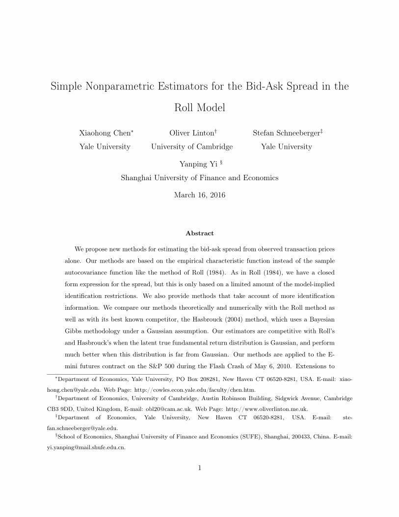
RMSE Bias Stdev q2.5 q25 q75 q97.5

εt ∼ 0.02N(0, 1)

secf 0.0154 -0.0002 0.0154 0.1690 0.1900 0.2100 0.2300secf,2 0.0156 -0.0002 0.0156 0.1680 0.1900 0.2100 0.2300secf,Σ0

−1 0.0528 0.0074 0.0523 0.1730 0.1920 0.2090 0.4345sRoll,1 0.0143 0.0003 0.0143 0.1713 0.1910 0.2100 0.2283sRoll,2 0.0143 0.0003 0.0143 0.1713 0.1910 0.2100 0.2283sHas.,1 0.1292 -0.0836 0.0986 0.0000 0.0000 0.2002 0.2031sHas.,n∗=2913 0.0019 -0.0001 0.0019 0.1961 0.1986 0.2011 0.2036

εt ∼ 0.02t(2)

secf 0.0164 0.0000 0.0164 0.1670 0.1890 0.2110 0.2320secf,2 0.0166 0.0000 0.0166 0.1670 0.1890 0.2110 0.2320secf,Σ0

−1 0.0498 0.0059 0.0495 0.1630 0.1890 0.2120 0.3515sRoll,1 0.0192 0.0006 0.0192 0.1661 0.1896 0.2115 0.2335sRoll,2 0.0184 0.0008 0.0184 0.1663 0.1897 0.2115 0.2336sHas.,1 0.0773 -0.0297 0.0714 0.0000 0.1967 0.2048 0.2120sHas.,n∗=4343 0.0289 -0.0039 0.0286 0.0693 0.1988 0.2054 0.2123

εt ∼ 0.02t(1)

secf 0.0186 -0.0009 0.0185 0.1610 0.1870 0.2120 0.2340secf,2 0.0187 -0.0010 0.0186 0.1610 0.1860 0.2120 0.2340secf,Σ0

−1 0.1031 0.0118 0.1025 0.0000 0.1470 0.2560 0.4970sRoll,1 0.2397 0.0514 0.2342 0.0000 0.1700 0.2580 1.1315sRoll,2 0.2410 0.0689 0.2310 0.0676 0.1772 0.2643 1.1652sHas.,1 0.2973 -0.0398 0.2946 0.0523 0.0673 0.1405 0.7770sHas.,n∗=4980 0.2976 -0.0392 0.2951 0.0530 0.0675 0.1408 0.7782

εt ∼ 0.02LN(0, 1.25)

secf 0.0167 -0.0008 0.0167 0.1660 0.1880 0.2110 0.2310secf,2 0.0168 -0.0008 0.0168 0.1650 0.1880 0.2110 0.2310secf,Σ0

−1 0.0656 0.0115 0.0646 0.1505 0.1880 0.2140 0.4580sRoll,1 0.0190 -0.0003 0.0190 0.1627 0.1881 0.2117 0.2354sRoll,2 0.0188 -0.0003 0.0188 0.1627 0.1881 0.2117 0.2355sHas.,1 0.0471 -0.0114 0.0457 0.0000 0.1987 0.2087 0.2165sHas.,n∗=4870 0.0348 -0.0064 0.0343 0.0719 0.1993 0.2088 0.2165

εt ∼ 0.02LN(0, 2)

secf 0.0214 -0.0017 0.0213 0.1550 0.1840 0.2130 0.2400secf,2 0.0215 -0.0017 0.0215 0.1550 0.1840 0.2130 0.2400secf,Σ0

−1 0.1383 -0.0023 0.1383 0.0000 0.0890 0.2720 0.5000sRoll,1 0.1591 0.0253 0.1571 0.0000 0.1631 0.2844 0.5210sRoll,2 0.1739 0.0591 0.1635 0.0672 0.1847 0.2961 0.5972sHas.,n∗=5000 0.1380 -0.0916 0.1032 0.0569 0.0747 0.1095 0.2808

Table 2: Simulation results for spread s0 = 0.2, sample size T = 250 and n = 5, 000 simulationruns. (See the caption of Table 1 for further details.)

19

4.2 An Application to E-mini S&P Futures Transaction Data

In this section we illustrate the usefulness of our estimator with an application to data on traded

E-Mini S&P futures contracts. These contracts are electronically traded futures contracts with the

S&P 500 stock market index as underlying, where the notional value of each contract is 50 times

the value of the S&P 500 index. The contracts are traded on the Chicago Mercantile Exchange’s

Globex electronic trading platform, where trading takes place from Sunday-Friday from 6 pm to 5

pm ET (Eastern Time), with a 15 min trading halt period Monday-Friday from 4:15 pm to 4:30

pm, and a maintenance period Monday-Thursday from 5 pm to 6 pm.7

In our application we look at the trading data for May 6, 2010.8 During this day, financial markets in

the U.S. experienced one of the most volatile periods on record, with major stock indices collapsing

and rebounded within a short time frame of less than an hour.9 Consequently, this episode has

become known as the Flash Crash (of 2010). For an illustration, Figure 1 displays the transaction

prices for the sample period: the left plot shows the trading price of the last trade in each second;

the right plot shows the sequence of all transaction prices. The difference in the two plots highlights

that the majority of the trading on May 6 happened around the time of the Flash Crash. For

comparison purposes, Figure 2 displays the same data for May 13, 2010, on which no unusual

market turbulence occurred. A joint report by the U.S. SEC and the U.S. CFTC (henceforth SEC-

CFTC report) published in 2010 identifies the market for E-mini S&P futures as one of the sources

of the turbulences:

"The combined selling pressure from the sell algorithm, HFTs, and other traders drove the price of

the E-Mini S&P 500 down approximately 3% in just four minutes from the beginning of 2:41 p.m.

through the end of 2:44 p.m. During this same time cross-market arbitrageurs who did buy the E-

Mini S&P 500, simultaneously sold equivalent amounts in the equities markets, driving the price of

SPY (an exchange-Transaction fund which represents the S&P500 index) also down approximately

3%."

This makes the E-mini futures market an interesting object to study. In particular, we want to

analyze how the liquidity cost of the E-mini S&P future evolved during the period of the Flash7Before September 21, 2015, E-mini contracts used to trade for 23 hours a day from 6 pm to 5:15 pm ET.8Specifically, we look at all trades from May 5, 6 pm to May 6, 4:15 pm ET.9For a more detailed description of the events on May 6, along with an in-depth empirical analysis, see, e.g.,

Kirilenko et al. (2014) or U.S. SEC & U.S. CFTC (2010).

20

Crash. We focus on the period from 2:32 pm to 3:08 pm ET (Kirilenko et al. (2014) date the Flash

Crash to this specific period), and we restrict our analysis to trades in the E-mini contract maturing

in June 2010 (this contract makes up 99.65% of the number of trades on that day). To measure the

liquidity cost, we estimate the implied spread with our estimator secf (with c = 0.1, ng = 12), as

well as with sRoll,1, i.e., Roll’s estimator with Hasbrouck (2009) correction. We do not report results

for sHas., since the underlying Gibbs sampling procedure (with the parameter configurations as in

the code of the author) only converged for about 20% of the cases in the (restricted) sample. The

method does not seem to handle high-frequency data well, which often involves consecutive trades

at identical prices and price bounces in discrete (tick-size) steps. This makes the price innovations a

discrete process, whereas Hasbrouck’s estimator is based on the assumption of Gaussian (and thus

continuous) innovations. This is consistent with two observations: first, the convergent cases are

concentrated around the most volatile subperiod, where the price innovations appear less discrete;

and second, adding a small Gaussian noise to the data makes the algorithm converge. For the

estimation we use a rolling-window approach, where we estimate the spread for each second, using

all trades over the last 30 seconds as input data (alternative window sizes of 15 or 20 seconds do

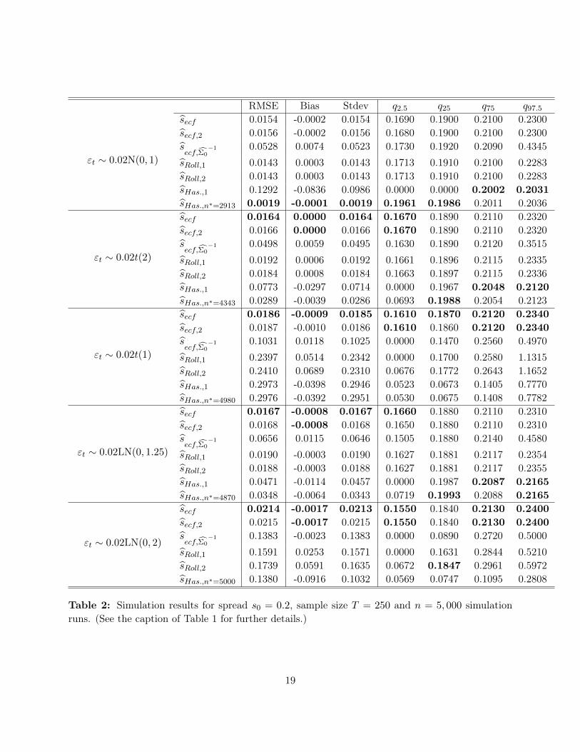
not change the results in a significant way). Figure 3 plots the corresponding prices and, for each

second, the number of trades in the last 30 seconds for our restricted sample period. We use log

prices to give the spread a relative percentage interpretation (given its magnitude, the results a

restated in basis points, BPS; 1 BPS = 1/100%). The results are presented in Figure 4 and can be

summarized as follows:

• Both estimators secf and sRoll,1 produce almost identical (and roughly constant) results

throughout the sample period, except for the time between 2:45 pm to 2:49 pm ET, dur-

ing which the spread appears to spike, and then returns to its previous level. However, the

increase is much more pronounced for sRoll,1 than for our estimator secf . The turbulence in

market prices during this period, along with the simulation evidence in the previous section

on the robustness of secf in a heavy-tailed environment, suggests that sRoll,1 might overstate

the (increase in the) underlying liquidity cost, and that secf provides a better approximation.

This is consistent with the fact that outside the window of extreme turbulence both methods

produce nearly identical results.

• The detected spike in the spread is consistent with the following passages in the SEC-CFTC

21

report: "HFTs, therefore, initially provided liquidity to the market. However, between 2:41

and 2:44 p.m., HFTs aggressively sold about 2,000 E-Mini contracts in order to reduce their

temporary long positions." The estimates seem to pick up this temporary liquidity evaporation,

although with some time lag.

• However, we do not find any detectable early warning signs of a pending crash in the spread

estimates. This is in contrast to, e.g., Easley et al. (2012), who find that the (appropriately

measured) market order flow became increasingly imbalanced in the hour preceding the crash,

and that this imbalance contributed to the withdrawal of many liquidity providers from the

market.

Figure 1: Transaction prices for E-Mini S&P futures (with maturity in June 2010) from May 5,

2010, 6 pm to May 6, 2010, 4:15 pm ET. Left: The last trading price for each second; Right: The

sequence of all transaction prices throughout the day.

22

Figure 2: Transaction prices for E-Mini S&P futures (with maturity in June 2010) from May 12,

2010, 6 pm to May 13, 2010, 4:15 pm ET. Left: The last trading price for each second; Right: The

sequence of all transaction prices throughout the day.

Figure 3: Transaction prices (left) and the number of trades in the last 30 seconds (right) for the

period of the Flash Crash.

23

Figure 4: Spread estimates secf (left) and sRoll,1 (right) for the period of the Flash Crash, with

approximate 95% confidence bands (gray area).

4.2.1 Estimating the c.f. of the Fundamental Price Innovations εt

We have emphasized the estimation of the bid-ask spread parameter s0, but it may also be of interest

to estimate features of the distribution of the innovation process. We obtain estimates of the c.f. of

the innovation process from (12) by using our spread estimator:

ϕε(u) :=ϕT,1(u)[

cos(usecf

2

)]2 .

The properties of this estimator follow directly from our analysis of secf and from the properties

of the sample characteristic function of the observed transaction prices. For an illustration, we

incorporate this estimator into our empirical analysis of the E-mini futures data. We estimate the

c.f. ϕε for three different points in time: before, at, and after the spike in the estimated spread (see

Figure 4); specifically, we choose the times 2:36 pm, 2:46 pm, and 2:56 pm ET, respectively. As in

the previous section, we use all transaction prices for the last 30 seconds in the estimation. We find

the following, with the estimates displayed in Figure 5:

• For 2:36 pm, we obtain an estimate that resembles the c.f. of a point mass at zero (i.e.,

a horizontal line), which is intuitive: the data shows that, during the tranquil periods of

trading, the executed transaction price jumps up or down (with roughly equal probability) by

24

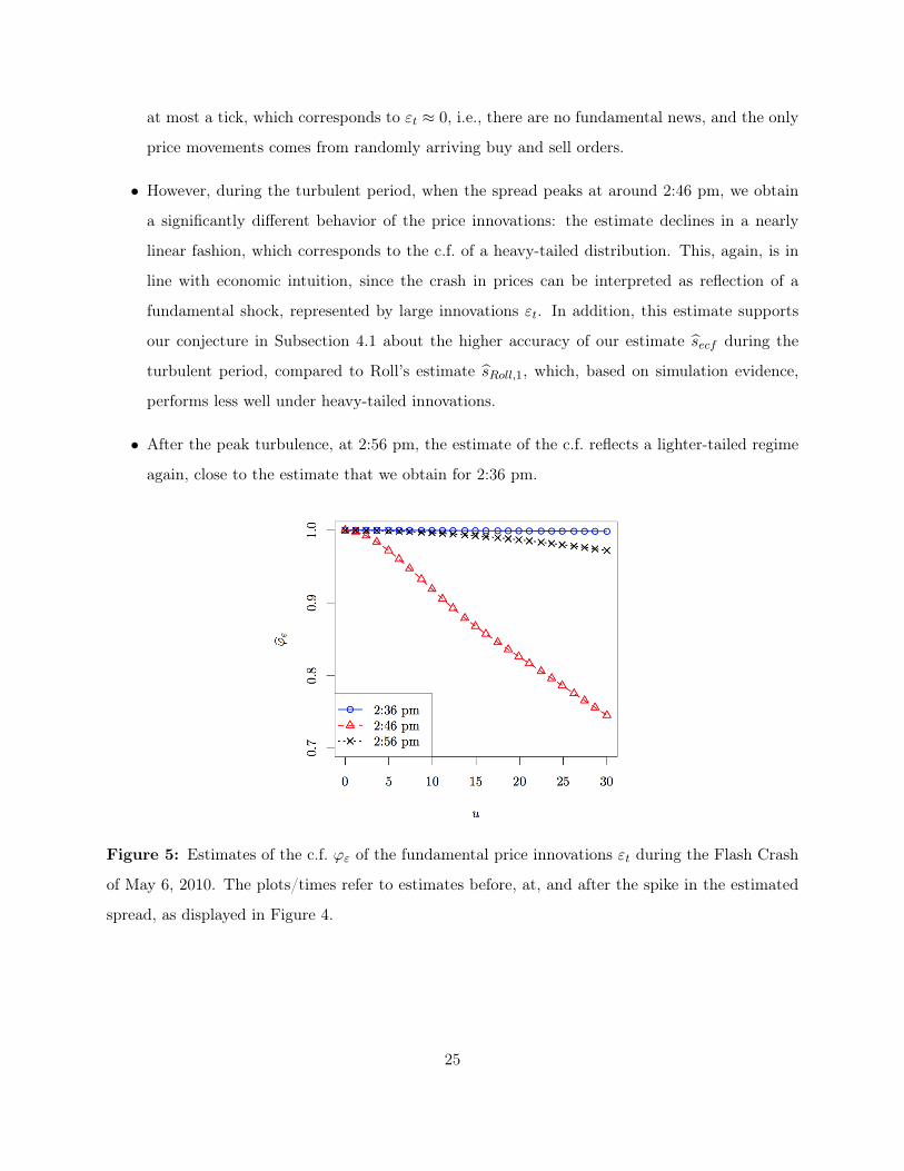
at most a tick, which corresponds to εt ≈ 0, i.e., there are no fundamental news, and the only

price movements comes from randomly arriving buy and sell orders.

• However, during the turbulent period, when the spread peaks at around 2:46 pm, we obtain

a significantly different behavior of the price innovations: the estimate declines in a nearly

linear fashion, which corresponds to the c.f. of a heavy-tailed distribution. This, again, is in

line with economic intuition, since the crash in prices can be interpreted as reflection of a

fundamental shock, represented by large innovations εt. In addition, this estimate supports

our conjecture in Subsection 4.1 about the higher accuracy of our estimate secf during the

turbulent period, compared to Roll’s estimate sRoll,1, which, based on simulation evidence,

performs less well under heavy-tailed innovations.

• After the peak turbulence, at 2:56 pm, the estimate of the c.f. reflects a lighter-tailed regime

again, close to the estimate that we obtain for 2:36 pm.

Figure 5: Estimates of the c.f. ϕε of the fundamental price innovations εt during the Flash Crash

of May 6, 2010. The plots/times refer to estimates before, at, and after the spike in the estimated

spread, as displayed in Figure 4.

25

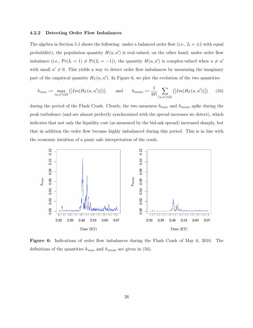
4.2.2 Detecting Order Flow Imbalances

The algebra in Section 5.1 shows the following: under a balanced order flow (i.e., It = ±1 with equal

probability), the population quantity H(u, u′) is real-valued; on the other hand, under order flow

imbalance (i.e., Pr(It = 1) 6= Pr(It = −1)), the quantity H(u, u′) is complex-valued when u 6= u′

with small u′ 6= 0. This yields a way to detect order flow imbalances by measuring the imaginary

part of the empirical quantity HT (u, u′). In Figure 6, we plot the evolution of the two quantities

hmax := max(u,u′)∈U

(∣∣Im(HT (u, u′))∣∣)) and hmean :=

1

|U|∑

(u,u′)∈U

(∣∣Im(HT (u, u′))∣∣) (34)

during the period of the Flash Crash. Clearly, the two measures hmax and hmean spike during the

peak turbulence (and are almost perfectly synchronized with the spread increases we detect), which

indicates that not only the liquidity cost (as measured by the bid-ask spread) increased sharply, but

that in addition the order flow became highly imbalanced during this period. This is in line with

the economic intuition of a panic sale interpretation of the crash.

Figure 6: Indications of order flow imbalances during the Flash Crash of May 6, 2010. The

definitions of the quantities hmax and hmean are given in (34).

26

5 Extensions

This section presents identification results for four extended models that relax parts of Assumption

1 imposed in Sections 2 and 3. The purpose is to show how we may accommodate more general

features in the basic Roll type model (1), and potentially how to estimate them from transaction

data {pt}Tt=1 alone, without further observed information.

5.1 Unbalanced Order Flow

Assumption 5. (i) Assumption 1(i)(ii) holds; and (ii) {It} takes values ±1 with unknown proba-

bility q0 := Pr(It = 1) ∈ (0, 1).

This relaxation allows for unbalanced order flow (i.e., q0 6= 1/2). Under Assumption 5, we obtain

the following relations (similar to Equations (5), (6) and (7) in Section 2): for all (u, u′) ∈ R2,

ϕ∆p,2(u, u′) = ϕε(u)ϕε(u′)E(

exp(ius0

2It

))E(

exp(i(u′ − u)

s0

2It−1

))E(

exp(−iu′ s0

2It−2

))= ϕε(u)ϕε(u

′)[cos(us0

2

)+ (2q0 − 1)i sin

(us0

2

)] [cos(u′s0

2

)− (2q0 − 1)i sin

(u′s0

2

)]×[cos(

(u′ − u)s0

2

)+ (2q0 − 1)i sin

((u′ − u)

s0

2

)],

ϕ∆p,1(u) = ϕ∆p,2(u, 0) = ϕε(u)[cos2

(us0

2

)+ (2q0 − 1)2 sin2

(us0

2

)],

ϕ∆p,2(u, u) = (ϕε(u))2[cos2

(us0

2

)+ (2q0 − 1)2 sin2

(us0

2

)].

In addition to the definitions of V, U and H(u, u′) given in Section 2, we introduce a function on

U × S × (0, 1) as

R(u, u′; s, q) :=

[cos(u s

2

)+ (2q − 1)i sin

(u s

2

)] [cos(u′ s

2

)− (2q − 1)i sin

(u′ s

2

)]×[cos((u′ − u) s

2

)+ (2q − 1)i sin

((u′ − u) s

2

)][cos2

(u s2)

+ (2q − 1)2 sin2(u s2)] [

cos2(u′ s2)

+ (2q − 1)2 sin2(u′ s2)] ,

which is complex-valued unless either u = u′ or (2q−1) sin(u′ s2)

= 0. In particular, R(u, u′; s, 1/2) =

R(u, u′; s) defined in Section 2. Similar to the identification Equation (14) for the basic Roll type

model in Section 2, we have:

H(u, u′) = R(u, u′; s0, q0) for all (u, u′) ∈ V2, (35)

27

and H(u, u′) is complex-valued unless either u = u′ or (2q0 − 1) sin(u′ s02

)= 0. Therefore for all

(u, u) ∈ V2 with u 6= 0, Equation (35) yields the relations

H(u, u) =1

cos2(u s02)

+ (2q0 − 1)2 sin2(u s02) ,

⇐⇒ cos2(us0

2

)=

1/H(u, u)− (2q0 − 1)2

1− (2q0 − 1)2, (36)

where H(u, u) is real-valued with H(u, u) > 1. Once (2q0 − 1)2 is identified or estimated, Equation

(36) can be used to identify or estimate s0 (as in Section 2). For (u,−u) ∈ V2 with u 6= 0, Equation

(35) implies

H(u,−u)

[H(u, u)]2=[cos(us0

2

)+ (2q0 − 1)i sin

(us0

2

)]2[cos (us0)− (2q0 − 1)i sin (us0)] .

Re

(H(u,−u)

[H(u, u)]2

)= (2q0 − 1)2 +

[(2q0 − 1)2 − 1

]cos2

(us0

2

) [1− 2 cos2

(us0

2

)]= 2(2q0 − 1)2 −H(u, u)−1 + 2

[H(u, u)−1 − (2q0 − 1)2

]21− (2q0 − 1)2

,

where the last equality uses the relation implied by Equation (36). Therefore,

(2q0 − 1)2 =Re(H(u,−u)

[H(u,u)]2

)+H(u, u)−1 − 2H(u, u)−2

2 + Re(H(u,−u)

[H(u,u)]2

)− 3H(u, u)−1

(37)

which can be used to identify and estimate (2q0 − 1)2.

Im

(H(u,−u)

[H(u, u)]2

)=[(2q0 − 1)2 − 1

](2q0 − 1) sin2

(us0

2

)sin (us0)

= 2(1− 2q0)(1−H(u, u)−1)

√1/H(u, u)− (2q0 − 1)2

1− (2q0 − 1)2

√1− 1/H(u, u)

1− (2q0 − 1)2, (38)

which can be used to identify the sign of 2q0 − 1 for a small u 6= 0. These arguments lead to the

following theorem.

Assumption 6. (i) Assumption 2(i) holds; (ii) either (a) U = U ; or (b) U ⊂ U , and ∃(u, u), (u,−u) ∈

U such that 0 < u < u, where u denotes the first positive zero of u 7→ mins∈S cos(u s2).

Theorem 6. (1) Let Assumption 5 hold. Then: the c.f. ϕε(·) is identified as (9) on V, and (s0, q0)

is identified by Equations (36), (37) and (38) with a small positive u ∈ V.

(2) Let Assumptions 5 and 6 hold. Then: (s0, q0) is identified as the unique solution to the minimum

distance criterion function based on Equation (35) evaluated on U .

28

In Theorem 6 part(2), the minimum distance criterion function can be constructed similar to

Equation (27). Then the consistency and the asymptotic normality are readily established similar

to Theorems 3, 4 and 5. In practice, a more limited objective of detecting when order flow is

unbalanced can be addressed by examining the imaginary part of H(u, u′) for u 6= u′ with small

u′ 6= 0, since for such cases, H(u, u′) is complex-valued when q0 6= 1/2 and is real-valued when

q0 = 1/2. This is what we implemented in the empirical application section 4.2.

5.2 Model when {It} has general discrete support

We now consider a generalization of the Roll model by relaxing Assumption 1(iii) on the support

of the latent trade direction indicators.

Assumption 7. (i) Assumption 1(i)(ii) holds; and (ii) {It} may take values in {−k1, . . . , 0, . . . ,+k2},

and Pr(It = −k1) > 0, Pr(It = +k2) > 0.

Here, k1 and k2 are positive integers, measuring the strength of the order flow. Assumption

7(ii) allows the case where Pr(It = 0) = 0 or Pr(It = 0) > 0. It also allows for asymmetric support

in the sense that k1 6= k2. Denote the unknown marginal probabilities of {It} as π0 = [~πl], where

πl = Pr(It = l) ≥ 0, for l = −k1, . . . , 0, . . . ,+k2 and∑

l πl = 1. Let ϕI(u) := E (exp (iuIt)) denote

the c.f. of It, which is analytic and is uniquely determined by the unknown π0. By the inversion

theorem, the unknown π0 is identified as long as its c.f. ϕI(·) is identified. Under Assumption 7(i)

(i.e., Assumption 1(i)(ii)), we obtain: for all (u, u′) ∈ R2,

ϕ∆p,2(u, u′) = ϕε(u)ϕε(u′)ϕI

(us0

2

)ϕI

((u′ − u)

s0

2

)ϕI

(−u′ s0

2

), (39)

ϕ∆p,1(u) = ϕε(u)ϕI

(us0

2

)ϕI

(−us0

2

), (40)

ϕ∆p,2(u, u) = ϕε(u)ϕε(u)ϕI

(us0

2

)ϕI

(−us0

2

). (41)

By Equations (41) and (40), the c.f. ϕε(·) is identified as (9) on V. Denote

R(u, u′; s0, π0) :=E(exp

[i s02 (u′ − u) It−1

])E(exp

[iu′ s02 It−1

])E(exp

[−iu s02 It−1

]) .Then Equations (39) and (40) imply the following relation:

H(u, u′) = R(u, u′; s0, π0) for all (u, u′) ∈ V2. (42)

Under Assumption7(ii), we prove in Appendix that Equation (42) identifies both s0 and ϕI(·).

29

Theorem 7. (1) Let Assumption 7(i) hold. Then the c.f. ϕε(·) is identified as (9) on V.

(2) Let Assumption 7(i)(ii) hold. Then: s0 and the c.f. ϕI(·) are identified.

We can jointly estimate s0 and π0 by essentially the same minimum distance strategy as in

Section 3 based on an empirical version of the identification equation (42). Recently Zhang and

Hodges (2012) consider a model where our Assumption 7(ii) is replaced by {It} having support in

{−λ,−1, 1, λ}. They do not study the identification issue but directly apply Bayesian Gibbs method

for estimation under the additional assumption of εt ∼ i.i.d. N(0, σε).

5.3 General model when {It} is a Stationary Markov Chain of Order 1

{It} could also be a stationary first-order Markov Chain with

Pr(It = j|It−1 = m) = qmj , for m = −k, . . . , 0, . . . ,+k, and j = −k, . . . , 0, . . . ,+k.

The probabilistic property of {It} is determined by the unknown transition matrix Q0 = [qmj ].

Denote the associated stationary marginal probabilities of {It} as π0 = [~πl], where πl = Pr(It = l),

for l = −k, . . . , 0, . . . ,+k and∑

l πl = 1.

Assumption 8. (i) Assumption 1(i) holds; (ii) {It} is strictly stationary first-order Markov, irre-

ducible and aperiodic; and (iii) {It} takes values in {−k, . . . , 0, . . . ,+k}, and Pr(It = l) > 0, for

l = −k, . . . , 0, . . . ,+k.

Since {It} is a strictly stationary, finite-state Markov chain, by Theorem 3.1 of Bradley (2005),

{It} being irreducible and aperiodic is equivalent to its being ψ−mixing or strongly mixing. And

under such condition, the mixing rates are (at least) exponentially fast. Assumption 8 (ii) is

assumed, because {∆pt} is observed to be stationary and display short memory in real data. Under

Assumption 8, we obtain for all (u, u′) ∈ R2,

ϕ∆p,1(u) = ϕε(u)E(

exp[ius0

2(It − It−1)

]),

ϕ∆p,2(u, u′) = ϕε(u)ϕε(u′)E(

exp[ius0

2(It − It−1)

]exp

[iu′s0

2(It−1 − It−2)

]).

Suppose θ0 = (s0,Q0) ∈ Θ ⊂ Rd. It follows that

H(u, u′) = R(u, u′; s0,Q0), for all (u, u′) ∈ V2, (43)

30

where

R(u, u′; s0,Q0) :=E(exp

[iu s02 (It − It−1)

]exp

[iu′ s02 (It−1 − It−2)

])E(exp

[iu s02 (It − It−1)

])E(exp

[iu′ s02 (It−1 − It−2)

]) .We can identify θ0 = (s0,Q0) ∈ Θ ⊂ Rd by considering lots of (u, u′) ∈ V2. We next establish identi-

fication. Let ϕ∆I (·, ·) denote the true unknown joint c.f. of (It−1 − It−2, It − It−1). In the following

lemma, we first establish the identification result for the joint distribution of (It−1 − It−2, It − It−1)

and the spread, i.e.(s0, ϕ∆I (·, ·)). Since {It} takes values in {−k, . . . , 0, . . . ,+k}, the support of

(It − It−1) is {−2k, . . . , 0, . . . ,+2k} and the joint support of (It−1 − It−2, It − It−1) is

(−2k, 0) · · · · · · · · · (−2k, 2k)

(−2k + 1,−1) (−2k + 1, 0) · · · · · · · · · (−2k + 1, 2k)

(−2k + 2,−2) (−2k + 2,−1) (−2k + 2, 0) · · · · · · · · · (−2k + 2, 2k)

.

.

....

.

.

....

.

.

....

.

.

.

(−1,−2k + 1) · · · · · · (−1, 0) · · · · · · (−1, 2k − 1) (−1, 2k)

(0,−2k) (0,−2k + 1) · · · · · · (0, 0) · · · · · · (0, 2k − 1) (0, 2k)

(1,−2k) (1,−2k + 1) · · · · · · (1, 0) · · · · · · (1, 2k − 1)

.

.

....

.

.

....

.

.

....

.

.

.

(2k − 2,−2k) · · · · · · · · · (2k − 2, 0) (2k − 2, 1) (2k − 2, 2)

(2k − 1,−2k) · · · · · · · · · (2k − 1, 0) (2k − 1, 1)

(2k,−2k) · · · · · · · · · (2k, 0)

.

(44)

When one uses Equation (43) for estimation, the joint support information given in Equation (44)

shall be used to improve efficiency. Denote the joint probability mass matrix of (It−1 − It−2, It − It−1)

as Q0∆I , which is a (4k+1)×(4k+1) matrix. Denote the row vectors of Q0 as Qj,· = [qj,−k, · · · , qj,k],

for j = −k, . . . , 0, . . . ,+k. The summation of each component of Qj,· equals to 1, according to the

definition. The following equation shows the connection between Q0∆I and Q0, π0 :

Q0∆I = AQ0,π0 ×BQ0 , (45)

where AQ0,π0 is a (4k + 1)× (2k + 1) matrix

πkqk,−k 0 0 0 · · · · · · 0

πk−1qk−1,−k πkqk,−k+1 0 0 · · · · · · 0

πk−2qk−2,−k πk−1qk−1,−k+1 πkqk,−k+2 0 · · · · · · 0

.

.

....

.

.

....

.

.

....

.

.

.

π−k+2q−k+2,−k π−k+3q−k+3,−k+1 π−k+4q−k+4,−k+2 · · · πkqk,k−2 0 0

π−k+1q−k+1,−k π−k+2q−k+2,−k+1 π−k+3q−k+3,−k+2 · · · πk−1qk−1,k−2 πkqk,k−1 0

π−kq−k,−k π−k+1q−k+1,−k+1 π−k+2q−k+2,−k+2 · · · πk−2qk−2,k−2 πk−1qk−1,k−1 πkqk,k

0 π−kq−k,−k+1 π−k+1q−k+1,−k+2 · · · πk−3qk−3,k−2 πk−2qk−2,k−1 πk−1qk−1,k

0 0 π−kq−k,−k+2 · · · πk−4qk−4,k−2 πk−3qk−3,k−1 πk−2qk−2,k

.

.

....

.

.

....

.

.

....

.

.

.

0 · · · 0 0 π−kq−k,k−2 π−k+1q−k+1,k−1 π−k+2q−k+2,k

0 · · · 0 0 0 π−kq−k,k−1 π−k+1q−k+1,k

0 · · · 0 0 0 0 π−kq−k,k

,

31

and BQ0 is (2k + 1)× (4k + 1) matrix

0 · · · · · · · · · 0 0 0 0 0 Q−k,·

0 · · · · · · · · · 0 0 0 0 Q−k+1,· 0

0 · · · · · · · · · 0 0 0 Q−k+2,· 0 0

.

.

....

.

.

....

.

.

....

.

.

....

.

.

....

0 · · · · · · · · · 0 0 Q−1,· · · · 0 0

0 · · · · · · · · · 0 Q0,· 0 · · · 0 0

0 · · · · · · 0 Q1,· 0 0 · · · 0 0

.

.

....

.

.

....

.

.

....

.

.

....

.

.

....

0 0 Qk−2,· 0 0 0 · · · · · · 0 0

0 Qk−1,· 0 0 0 0 · · · · · · 0 0

Qk,· 0 0 0 0 0 · · · · · · 0 0

.

Thus the rank of Q0∆I is at most 2k + 1. Since it does not satisfy the non-singularity condition,

Theorem 1 of Gassiat and Rousseau (2016) could not be applied to our case. Once ϕ∆I (·, ·) or

equivalently Q0∆I is identified and estimated, Equation (45) can be used to recover Q0 and π0.

Assumption 9. (i) AQ0,π0 is of full column rank; and (ii) q−k,−k > 12 and qk,k > 1

2 .

For example, if πkqk,j > 0, for j = −k, · · · , k, or π−kq−k,j > 0, for j = −k, · · · , k, then

Assumption 9(i) is satisfied. Also, when k = 1 (as in the basic Roll model), Assumption 9(ii) could

be interpreted as a model of (time-varying) autocorrelation in the trade indicators: after a buy, the

most likely thing is another buy, and analogously for a sell.

Lemma 1. Suppose that Assumptions 8 and 9 hold. Then on V2, (s0, ϕ∆I (·, ·)) and the c.f. ϕε are

uniquely identified.

In general, (s0, ϕ∆I (·, ·)) cannot be identified, without information about the support.

Example 5.1. {It} could take values in {−2,−1, 0, 1, 2}. The marginal distribution satisfies Pr(It =

−1) = Pr(It = 1) = 1/2, and the transition matrix is [1/3 2/3; 2/3 1/3]. DefineWt = 1/2 [It − It−1 + et],

with {et} being independent of {It}, and Pr(et = −2) = b,Pr(et = 2) = 1 − b. It is easy to show

the joint support of (Wt−1,Wt) is a subset of Equation (44) for k = 2. Therefore, Equation (43)

cannot distinguish (s, ϕ∆I (·, ·)) from (2s, ϕW (·, ·)), where ϕW (·, ·) is the joint c.f.of (Wt−1,Wt).

Simple calculations show Pr(Wt−1 = −2,Wt = −1) = Pr(Wt−1 = −1,Wt = −2) = 19b

2 > 0,

Pr(Wt−1 = 1,Wt = 2) = Pr(Wt−1 = 2,Wt = 1) = 19(1− b)2 > 0. If one has additional information

that Pr(It = −2) = Pr(It = 2) = 0, then it is known that (−2,−1), (−1,−2), (1, 2), (2, 1), are not

in Equation (44) for k = 1. Thus one is able to distinguish (s, ϕ∆I (·, ·)) from (2s, ϕW (·, ·)). More

32

generally, let Wt = c [It − It−1 + et], where c is any constant and {et} is independent of {It}. The

joint support of (Wt−1,Wt) is not a subset of Equation (44) for k = 1.

We next establish the identification results for the joint distribution of (It−1, It).

Theorem 8. Suppose that Assumptions 8 and 9 hold. Furthermore, qk,−j > 0, for j = 1, · · · , k and

q−k,j > 0, for j = 0, 1, · · · , k. Then s0 and the joint distribution of (It−1, It) are uniquely identified.

Lemma 1 shows the identification result for Q0∆I . Since Q0

∆I = AQ0,π0 × BQ0 , we show in the

proof of Theorem 8 that BQ0 or equivalently the joint distribution of (It−1, It) can be solved back

under some conditions on AQ0,π0 . Theorem 8 only gives one such sufficient condition.

5.4 Adverse Selection

In all the above extensions we have assumed that the price dynamics follows Equation (1). We now

relax this condition and suppose that

∆pt = εt + α0It − β0It−1, (46)

where the other parts of Assumption 1 are kept. This equation arises from considering the presence

of an adverse selection component in the spread, see Equation (5.4) in Foucault et al. (2013). In

this case, β0 = s0/2 and α0 = s0/2 + δ, where δ = α0 − β0 6= 0 measures the contribution of

adverse selection. Rewriting (46) in the form of our previous price dynamics in (1), i.e., ∆pt =

εt + (It − It−1)s0/2, we have εt = εt + δIt, and thus Cov (εt, It) = δ 6= 0, so that our estimator

(and the Roll and Hasbrouck estimators) would be biased. Under only autocovariance restrictions

and without trade direction data, (α0, β0, σ2ε) cannot be jointly identified (even under Hasbrouck

(2004)’s assumption of εt ∼ i.i.d. N(0, σε)). We now show how to obtain identification under

Hasbrouck (2004)’s stronger independence assumption that {εt} is independent of {It}.

Assumption 10. (i) Data {pt}Tt=1 is generated from Equation (46) with β0 > 0, where {εt} is i.i.d.

and independent of {It}; (ii) Assumption 1(ii)(iii) holds.

This assumption implies that for all (u, u′) ∈ R2,

ϕ∆p,2(u, u′) = ϕε(u)ϕε(u′)E (exp (iuα0It))E

(exp

(i(u′α0 − uβ0)It−1

))E(exp

(−iu′β0It−2

))= ϕε(u)ϕε(u

′) cos (uα0) cos(u′α0 − uβ0

)cos(u′β0

), (47)

ϕ∆p,1(u) = ϕ∆p,2(u, 0) = ϕε(u) cos (uα0) cos (uβ0) . (48)

33

Denote

Uas :=

{(u, u′) ∈ V2 : min

(α,β)∈S2| cos (uβ) cos

(u′α)| > 0

}, (49)

and a function on Uas × S2 as

R(u, u′;α, β) :=cos (u′α− uβ)

cos (uβ) cos (u′α)= 1 +

sin (uβ) sin (u′α)

cos (uβ) cos (u′α).

Equations (47) and (48) now imply that

H(u, u′) = R(u, u′;α0, β0) for (u, u′) ∈ V2, (50)

and hence H(u, u′) is real-valued for all (u, u′) ∈ V2. Since V2 contains an open ball of (0, 0), for a

small positive u ∈ V, we have (u, u), (u, 2u), (2u, u) ∈ V, and Equation (50) yields

sin2(uα0) =2H(u, u)−H(u, 2u)− 1

2H(u, u)− 2H(u, 2u), (51)

sin2(uβ0) =2H(u, u)−H(2u, u)− 1

2H(u, u)− 2H(2u, u). (52)

Since 0 < u < u2 , s 7→ sin2 (us) is strictly increasing in s ∈ S. This implies that (51) and (52) hold

only at α = α0 and β = β0. Consequently,

α0 = u−1 arcsin

(√2H(u, u)−H(u, 2u)− 1

2H(u, u)− 2H(u, 2u)

), β0 = u−1 arcsin

(√2H(u, u)−H(2u, u)− 1

2H(u, u)− 2H(2u, u)

).

Assumption 11. (i) (α0, β0) ∈ S2; (ii) either (a) U = Uas; or (b) U ⊂ Uas and ∃(u, u), (u, 2u), (2u, u) ∈

U , such that 0 < u < u2 , where u denotes the first positive zero of u 7→ mins∈S cos (us).

Theorem 9. (1) Let Assumption 10 hold. Then: (α0, β0) is identified by Equations (51) and (52)

for a small positive u ∈ V, and the c.f. ϕε is identified on V as ϕε(u) =ϕ∆p,1(u)

cos(uα0) cos(uβ0) .

(2) Let Assumptions 10 and 11 hold. Then: (α0, β0) is identified as the unique solution to the

minimum distance criterion function based on Equation (50) evaluated on U .

From this we can identify (s0, δ) jointly. In Theorem 9 part (2), the minimum distance criterion

function can be constructed similar to Equation (27). The consistency and the asymptotic normality

are readily established similar to Theorems 3, 4 and 5. We note that, with additional data such

as trade volume, the independence between {εt} and {It} condition in Assumption 10 could be

dropped. Furthermore, one could modify some recently development in nonclassical measurement

error (see, e.g., Hu (2016), Carroll et al. (2006)) to obtain further extensions of the basic Roll model.

34

6 Conclusions

In this paper we provide simple nonparametric estimators of the spread parameter using transaction

price data alone. We compare our method theoretically and numerically with the Roll (1984) method

as well as with the Hasbrouck (2004) method. Our estimators perform similarly to theirs when the

latent true fundamental return distribution is Gaussian, but much better than theirs when the

distribution is far from Gaussian, such as for high-frequency data.

In our application to the E-mini futures contract on the S&P 500 during the Flash Crash, we

find that during relatively tranquil times our estimator secf and the Roll estimator sRoll,1 are very

similar, but during the peak period of the Flash Crash, i.e., between 2:45 pm to 2:49 pm ET,

the spread appears to spike, and then returns to its previous level, but the increase is much more

pronounced for the Roll estimator than for our estimator. The turbulence in market prices during

this period, along with the simulation evidence on the robustness of our estimator secf in a heavy-

tailed environment, suggests that sRoll might overstate the (increase in the) underlying liquidity

cost, and that secf provides a better approximation. This is consistent with the fact that outside

the window of extreme turbulence both methods produce nearly identical results. We also found

that order flow became badly unbalanced. Both of these findings corroborate the work presented

in the SEC/CFTC report on the days events and subsequent academic work. We also find however

that the fundamental innovation became much more heavy tailed during the critical period, so that

perhaps explanations are not just due to market structure related issues.

We have emphasized in the theoretical treatment the plain Roll model, but we also showed

how certain extensions such as unbalanced order flow, or serially dependent latent trade indicators,

or adverse selection can be well accommodated in our framework. In fact, it may be possible to

consider further extensions that allow several features all at once, and one could consider more

efficient estimators as well. We leave these for future work.

35

Appendices

The Appendices consist of all the proofs and additional figures.

A. Proofs for Identification Results in Sections 2 and 5

Proof of Theorem 2 Both criterion functions (18) and (19) are nonnegative, with J(s0,U) =

Q(s0,U) = 0, under Assumption 2(ii). For either case of Assumption 2(ii), ∃(u, u) ∈ U with u > 0.

For this grid point, the moment condition (15) yields the relation

cos2(us0

2

)=

ϕ2∆p,1(u)

ϕ∆p,2(u, u). (53)

By Assumption 2(ii), u is smaller than the first positive zero of u 7→ mins∈S cos(u s2), and hence

s 7→ cos2(u s2)is strictly decreasing in s ∈ S. This implies that (53) holds only at s = s0, which

further implies that both criterion functions are uniquely minimized at s = s0. This gives the

identification result. Proof of Theorem 7

Let ϕI denote the c.f.of {It} associated with the true unknown π0, which is analytic on R, since

{It} is discrete with support {−k1, . . . , 0, . . . ,+k2}. Equation (42) gives on V2,

H(u, u′) =ϕI(s02 (u′ − u)

)ϕI(s02 u′)ϕI(− s0

2 u) . (54)

If the pair (s ∈ S, ψ(·)) also satisfies Equation (42), where ψ denotes the c.f.of {It} associated with

another probability mass function π i.e.,

H(u, u′) =ϕI(s02 (u′ − u)

)ϕI(s02 u′)ϕI(− s0

2 u) =

ψ(s2 (u′ − u)

)ψ(s2u′)ψ(− s

2u) . (55)

Below we shall prove that ϕI( s02 u) = exp(ifu)ψ(s2u), where f ∈ R is a constant, with no infor-

mation about the support of {It}. This result is intuitive. Since we only have observations fors02 (It − It−1), we could not differentiate between It and It + f , for a constant f , or between (It, s0)

and (It · s0s , s), for a positive constant s, without additional information about the support. Assump-

tion 7 (ii) excludes the possibility of a change of the location or the scale, then θ0 = (s0, πᵀ

0)ᵀ can be

uniquely identified from Equation (42). Denote h(u) = ψ(ss0u), and u1 = − s0

2 u, u2 = s02 u′. Note

that ϕI(·), ψ(·), h(·) are analytic on R and equal to 1 at 0. There exists a small neighbourhood

M of (0, 0) ⊂ V2, such that ϕI (u1), ϕI (u2), ϕI (u1 + u2), h (u1), h (u2) and h (u1 + u2) are all

36

bounded away from zero on (u1, u2) ∈M. Equation (55) gives

ϕI (u1 + u2)

h (u1 + u2)=ϕI (u1)

h (u1)

ϕI (u2)

h (u2). (56)

Define γ(u) = ϕI(u)h(u) , which is analytic on an open interval of 0. Equation (56) can be rewritten as

γ(u1 + u2) = γ(u1)γ(u2). (57)

In Theorem 1 on page 38 of Aczel (1966), it has been shown that the only nonzero analytic solutions

of (57) are the exponential functions, exp(au), where a ∈ C is a constant. Namely, ϕI( s02 u) =

exp(au)ψ(s2u), for some fixed a ∈ C. Since, for all u ∈ R, ϕI(− s0

2 u) = ϕI(s02 u) and ψ

(− s

2u)

=

ψ(s2u), it is straightforward to show a = if , for some f ∈ R. Equivalently,

s0

2It =

s

2It + f, (58)

where the c.f. of It is ϕI(u), and the c.f. of It is ψ (u). Equation (58) implies the number of points in

the support of It is also identified. Let the ordered sets {m1,m2, · · · ,ml} ⊂ {−k1, · · · , 0, · · · ,+k2}

and {m1, m2, · · · , ml} ⊂ {−k1, · · · , 0, · · · ,+k2} denote the supports of It and It, respectively. Equa-

tion (58) implies, for all i = 1, · · · , l,

mi =s0

smi − f

2

s.

Since m1 = m1 = −k1, and ml = ml = +k2, s0 = s and f = 0. Therefore, s0 and the distribution

of It can be uniquely identified. Then ϕε(u) =ϕ∆p,1(u)

ϕI(s02u)ϕI(− s0

2u). Proof of Lemma 1

Equation (43) gives on V2,

H(u1, u2) :=ϕ∆I

(s02 u1,

s02 u2

)ϕ∆I

(s02 u1, 0

)ϕ∆I

(0, s02 u2

) .If the pair (s, ψ∆I (·, ·)) also satisfies Equation (43), i.e.,

H(u1, u2) =ϕ∆I

(s02 u1,

s02 u2

)ϕ∆I

(s02 u1, 0

)ϕ∆I

(0, s02 u2

) =ψ∆I

(s2u1,

s2u2

)ψ∆I

(s2u1, 0

)ψ∆I

(0, s2u2

) . (59)

Then on V2, which contains a small neighbourhood of (0, 0)

ϕ∆I

(s0

2u1,

s0

2u2

)ψ∆I

(s

2u1, 0

)ψ∆I

(0,s

2u2

)= ψ∆I

(s

2u1,

s

2u2

)ϕ∆I

(s0

2u1, 0

)ϕ∆I

(0,s0

2u2

).

(60)

37

Since {It} is discrete with support {−k, . . . , 0, . . . ,+k}, ϕ∆I (·, ·) and ψ∆I (·, ·) are analytic. There-

fore ϕ∆I (·, ·) and ψ∆I (·, ·) have analytic continuations for all complex numbers (z1, z2) ∈ C2. Fur-

thermore, the analytic continuations, ϕ∆I (z1, z2) and ψ∆I (z1, z2) are entire functions, and Equation

(60) is satisfied for all (z1, z2) ∈ C2. Let Z ⊂ C be the set of zeros of ϕ∆I

(s02 ·, 0

), and Z ⊂ C be

the set of zeros of ψ∆I

(s2 ·, 0

). Fix z1 = d+ fi ∈ Z, where d, f ∈ R. Then, for any z ∈ C,

ϕ∆I

(s0

2z1,

s0

2z)ψ∆I

(s

2z1, 0

)ψ∆I

(0,s

2z

)= 0 (61)

Define a(z) =(exp

[iz s02 (−2k)

], · · · , exp

[iz s02 (−1)

], 1, exp

[iz s02 (1)

], · · · , exp

[iz s02 (2k)

])ᵀ, thenϕ∆I

(s0

2z1,

s0

2z)

= a(z)ᵀQ∆Ia(z1) = a(z)ᵀAQ,πBQa(z1).

z → ϕ∆I

(s02 z1,

s02 ·)is the null function if and only if AQ,πBQa(z1) = 0. Since AQ,π is of full

column rank, AQ,πBQa(z1) = 0 if and only if BQa(z1) = 0.

BQa(z1) =

q−k,−k + q−k,−k+1 exp(iz1

s02

)+ q−k,−k+2 exp

(2iz1

s02

)+ · · ·+ q−k,k exp

(2kiz1

s02

)q−k+1,−k exp

(−iz1 s02

)+ q−k+1,−k+1 + q−k+1,−k+2 exp

(iz1

s02

)+ · · ·+ q−k+1,k exp

((2k − 1)iz1

s02

)q−k+2,−k exp

(−2iz1

s02

)+ q−k+2,−k+1 exp

(−iz1 s02

)+ q−k+2,−k+2 + · · ·+ q−k+2,k exp

((2k − 2)iz1

s02

)...

......

...

qk−2,−k exp((−2k + 2)iz1

s02

)+ · · ·+ qk−2,k−2 + qk−2,k−1 exp

(iz1

s02

)+ qk−2,k exp

(2iz1

s02

)qk−1,−k exp

((−2k + 1)iz1

s02

)+ qk−1,−k+1 exp

((−2k + 2)iz1

s02

)+ · · ·+ qk−1,k−1 + qk−1,k exp

(iz1

s02

)qk,−k exp

(−2kiz1

s02

)+ qk,−k+1 exp

((−2k + 1)iz1

s02

)+ qk,−k+2 exp

((−2k + 2)iz1

s02

)+ · · ·+ qk,k

The real part of the first component of BQa(z1) equals to

q−k,−k + q−k,−k+1 exp(−f

s0

2

)cos

ds0

2+ q−k,−k+2 exp

(−2f

s0

2

)cos

2ds0

2+ · · ·+ q−k,k exp

(−2kf

s0

2

)cos

2kds0

2, (62)

while the real part of the last component of BQa(z1) equals to

qk,−k exp(

2kfs0

2

)cos

2kds0

2+ qk,−k+1 exp

((2k − 1)f

s0

2

)cos

(2k − 1)ds0

2+ · · ·+ qk,k−1 exp

(fs0

2

)cos

ds0

2+ qk,k. (63)

Since qk,k > 1/2 and q−k,−k > 1/2, either Equation (62) or (63) is strictly larger than zero, no

matter what value z1 takes. Therefore, AQ,πBQa(z1) 6= 0 and z → ϕ∆I

(s02 z1,

s02 ·)is not the null

function. Thus, it is possible to choose z2 ∈ C such that ϕ∆I

(s02 z1,

s02 z2

)6= 0, and ψ∆I

(0, s2z2

)6= 0.

Then Equation (61) leads to ψ∆I

(s2z1, 0

)= 0, therefore Z ⊂ Z. A similar argument shows Z ⊂ Z,

therefore Z = Z. Since ϕ∆I

(s02 z, 0

)and ψ∆I

(s2z, 0

)have growth order 1, using Hadamard’s

factorization theorem (see Stein and Shakarchi (2003), Theorem 5.1), we can get that there exists

a polynomial R of degree ≤ 1 such that for all z ∈ C,

ϕ∆I

(s0

2z, 0)

= exp(R(z))ψ∆I

(s

2z, 0

).

38

Since ϕ∆I (0, 0) = ψ∆I (0, 0) = 1, there exists a complex number c such that ϕ∆I

(s02 z, 0

)=

exp(cz)ψ∆I

(s2z, 0

). Furthermore, for all z ∈ R, ϕ∆I

(− s0

2 z, 0)

= ϕ∆I

(s02 z, 0

)and ψ∆I

(− s

2z, 0)

=

ψ∆I

(s2z, 0

). It is straightforward to show c = if , for some f ∈ R. According to the support

information, the only possible value of f is zero. Therefore, ϕ∆I

(s02 z, 0

)= ψ∆I

(s2z, 0

), for all

z ∈ C. Since ϕ∆I

(s02 z, 0

)= ϕ∆I

(0, s02 z

), and ψ∆I

(s2z, 0

)= ψ∆I

(0, s2z

), Equation (60) leads

to ϕ∆I

(s02 z1,

s02 z2

)= ψ∆I

(s2z1,

s2z2

), for all (z1, z2) ∈ C2. Namely, the joint distribution of[

s02 (It−1 − It−2), s02 (It − It−1)

]can be identified by Equation (43). According to the joint support

information of (It−1 − It−2, It − It−1), s0 can be identified. Therefore, (s0, ϕ∆I (·, ·)) is identified.

Then ϕε(u) =ϕ∆p,1(u)

ϕ∆I(s02u,0)

. Proof of Theorem 8

According to Lemma 1, s0 and the joint distribution of (It−1 − It−2, It − It−1) can be identified by

Equation (43). For any fixed integer k, {It} takes values in {−k, · · · , 0, · · · ,+k). The probabilities

of the first row and the last row of Equation (44) satisfy

Pr(−2k, j) = πkqk,−kq−k,−k+j , Pr(2k,−j) = π−kq−k,kqk,k−j , for j = 0, 1, · · · , 2k

where Pr(−2k, j) and Pr(2k,−j) are short for Pr(It−1 − It−2 = −2k, It − It−1 = j) and Pr(It−1 −

It−2 = 2k, It − It−1 = −j), respectively. Along with the fact that∑2k

j=0 q−k,−k+j = 1 and∑2kj=0 qk,k−j = 1, πk, π−k, Qk, · and Q−k, · can be identified. The probabilities of the second

row and the second last row of Equation (44) satisfy

Pr(−2k + 1,−1) = πkqk,−k+1q−k+1,−k, Pr(−2k + 1, 2k) = πk−1qk−1,−kq−k,k, (64)

Pr(−2k + 1, j) = πkqk,−k+1q−k+1,−k+j+1 + πk−1qk−1,−kq−k,−k+j , for j = 0, 1, · · · , 2k − 1 (65)

Pr(2k − 1, 1) = π−kq−k,k−1qk−1,k, Pr(2k − 1,−2k) = π−k+1q−k+1,kqk,−k, (66)

Pr(2k − 1,−j) = π−kq−k,k−1qk−1,k−1−j + π−k+1q−k+1,kqk,k−j , for j = 0, 1, · · · , 2k − 1 (67)

Equation (64) and (66) can be used to identify πk−1×qk−1,−k, π−k+1×q−k+1,k, qk−1,k and q−k+1,−k.

Then Equation (65) and (67) can be used to identify q−k+1,j , for j = −k + 1, · · · , k and qk−1,j , for

j = −k, · · · , k − 1, respectively. Consequently, πk−1 and π−k+1 can be identified. Following the

same strategy, the probabilities of the third row and the third last row of Equation (44) can be

used to identify πk−2, π−k+2, Qk−2, · and Q−k+2, ·. Essentially, the same strategy can be applied

recursively to identify π and Q.

39

B. Proofs for Estimation Results in Section 3

We start with some background material. The complex conjugate and the real and imaginary

parts of a complex number z are denoted by z, Re(z), and Im(z), respectively. Denote the joint

characteristic function and empirical c.f. of(∆pt, · · · ,∆pt−(d−1)

), for d ≥ 1, by

ϕ∆p,d (u1, u2, · · · , ud) = E(exp

(iu1∆pt + iu2∆pt−1 + · · ·+ iud∆pt−(d−1)

)), (68)

ϕT,d (u1, u2, · · · , ud) =1

T

T∑t=1

exp(iu1∆pt + iu2∆pt−1 + · · ·+ iud∆pt−(d−1)

), (69)

where E (ϕT,d (u1, u2, · · · , ud)) = ϕ∆p,d (u1, u2, · · · , ud). Define the empirical characteristic function

process

WT,2

(u, u′

):=√T(ϕT,2

(u, u′

)− ϕ∆p,2

(u, u′

))(70)

Concerning the covariance structure, since {∆pt}Tt=1 is strictly stationary and 1-dependent, we are

able to show that

limT→∞

Cov(WT,2

(u, u′

),WT,2

(v, v′

))=

2∑s=−2

Cov[exp

(iu∆pt + iu′∆pt−1

), exp

(iv∆pt−s + iv′∆pt−s−1

)]=

ϕ∆p,4 (−v,−v′, u, u′) + ϕ∆p,4 (u, u′,−v,−v′) + ϕ∆p,3 (−v, u− v′, u′) + ϕ∆p,3 (u, u′ − v,−v′)

+ϕ∆p,2 (u− v, u′ − v′)− 5ϕ∆p,2 (u, u′)ϕ∆p,2 (−v,−v′) ,

(71)

which can be consistently estimated by the sample analogs. Given {∆pt}Tt=1 is strictly stationary and

1-dependent, following Theorem 2.1 and Theorem 2.2 of Feuerverger (1990), we have the following

result:

Lemma 2. For d ≥ 1,

(i) ϕT,d (u1, u2, · · · , ud)→ ϕ∆p,d (u1, u2, · · · , ud) a.s., ∀ (u1, u2, · · · , ud) ∈ Rd;

(ii) sup|uj |≤M, j=1,··· ,d |ϕT,d (u1, u2, · · · , ud)−ϕ∆p,d (u1, u2, · · · , ud) | → 0 a.s., for any fixed 0 < M <∞;

(iii) ∀k, ∀ (u1, u′1) , · · · , (uk, u′k) ∈ R2 :

(WT,2

(u1, u

′1

), · · · ,WT,2

(uk, u

′k

))→d

(W2

(u1, u

′1

), · · · ,W2

(uk, u

′k

)),

where {W2 (u, u′) = W2 (−u,−u′), (u, u′) ∈ R2} is a zero mean complex-valued Gaussian process

with the covariance structure (71).

40

Proof of Theorem 3 Under Assumption 2′, S is compact and U contains only finite number of

grid points. It is straightforward to show sups∈S |JT (s,U) − J (s,U) | = op(1), due to the fact

that the characteristic functions are bounded by unity in norm and Lemma 2(ii). In addition, the

identification result in Theorem 2 establishes J (s,U) > 0, for s ∈ S, s 6= s0. Then using Theorem

2.1 of Newey and McFadden (1994), the consistency of secf is established. Assumptions 1 and 2′

assure that inf(u,u′)∈U |ϕ∆p,1(u)ϕ∆p,1(u′)| > 0, or equivalently

sup(u,u′)∈U | 1ϕ∆p,1(u)ϕ∆p,1(u′) | <∞. Along with Lemma 2 and the property of characteristic functions,

we are able to show sup(u,u′)∈U |HT (u, u′) − H(u, u′)| = op(1). Also, H(u, u′) = R(u, u′; s0) is

uniformly bounded on U . Then the consistency of secf,2 can be established similarly. Assumptions

1 and 2′ also ensure that

min(u,u′)∈U

(|ϕ2

∆p,1(u)|, |ϕ2∆p,1(u′)|, |ϕ∆p,2(u, u)|, |ϕ∆p,2(u′, u′)|

)≥ δ1 > 0,

for some constant δ1. This establishes that, as stated in Remark 1, if the cutoff c in the construction

of U is chosen small enough (c < δ1), then the corresponding trimming constraints I{|ϕ2T,1(u)| > c

}and I {|ϕT,2(u, u)| > c} are not binding asymptotically. Before we

prove Theorem 4 on the asymptotic normality, we define quantities that appear inside the limiting

variances of our estimators. Let W2 (u, u′) be a Gaussian process with covariance function

cov(W2

(u, u′

),W2

(v, v′

))(72)

= ϕ∆p,4

(−v,−v′, u, u′

)+ ϕ∆p,4

(u, u′,−v,−v′

)+ ϕ∆p,3

(−v, u− v′, u′

)+ ϕ∆p,3

(u, u′ − v,−v′

)+ ϕ∆p,2

(u− v, u′ − v′

)− 5ϕ∆p,2

(u, u′

)ϕ∆p,2

(−v,−v′

),

where the joint c.f. of(∆pt, . . . ,∆pt−(d−1)

), for d ≥ 1, is denoted by ϕ∆p,d (u1, u2, . . . , ud) =

E(exp

(iu1∆pt + iu2∆pt−1 + · · ·+ iud∆pt−(d−1)

)). Define the real random variables

G(u, u′) := Re

(W2 (u, u′)

ϕ∆p,1(u)ϕ∆p,1(u′)

)−R(u, u′; s0) Re

(W2 (0, u′)

ϕ∆p,1(u′)

)−R(u, u′; s0) Re

(W2 (u, 0)

ϕ∆p,1(u)

)(73)

= 12

[W2(u,u′)

ϕ∆p,1(u)ϕ∆p,1(u′) + W2(−u,−u′)ϕ∆p,1(−u)ϕ∆p,1(−u′)

]− R(u,u′;s0)

2

[W2(0,u′)ϕ∆p,1(u′) + W2(0,−u′)

ϕ∆p,1(−u′) + W2(u,0)ϕ∆p,1(u) + W2(−u,0)

ϕ∆p,1(−u)

].

Denote the vectorized version of {G(u, u′);∀(u, u′) ∈ U} as G(U). Let the covariance of G(U) be

Σ0, which is a |U| × |U| matrix. Every component of Σ0, cov (G(u, u′), G(v, v′)), can be calculated

using (72). We provide a detailed instruction on how to calculate Σ0 and a consistent estimator Σ0

41

in Appendix C. Proof of Theorem 4 In the proof, we shall verify the conditions in Theorem 3.1

of Newey and McFadden (1994) for the asymptotic normality. In the following ∇s and ∇ss denote

the first and second derivatives of a function with respect to s, respectively. We first derive a few

useful formulae.

∇sR(u, u′; s) =u′

2 sin(u s2)

cos(u s2)

+ u2 sin

(u′ s2)

cos(u′ s2)[

cos(u s2)

cos(u′ s2)]2 , (74)

∇ssR(u, u′; s) =

uu′

2 cos(u s2)

cos(u′ s2)

+ sin(u s2)

sin(u′ s2) (

u′2

2 cos2(u s2)

+ u2

2 cos2(u′ s2))

[cos(u s2)

cos(u′ s2)]3 .

Note that on the boundary point 0, ∇sR(u, u′; 0) ≡ 0, ∀(u, u′) ∈ U . Under Assumption 2′ (ii),

sup(u,u′)∈U ,s∈S

|∇sR(u, u′; s)| < M3, sup(u,u′)∈U ,s∈S

|∇ssR(u, u′; s)| < M4, (75)

for some fixed number 0 < M3,M4 <∞.

(i) We have

∇ssJ (s0,U) = 2∑

(u,u′)∈U

|ϕ∆p,1(u)|2|ϕ∆p,1(u′)|2 ∇2sR(u, u′; s0) > 0 (76)

∇sJT (s,U) = −2∑

(u,u′)∈U

∇sR(u, u′; s) Re(ϕT,1(u)ϕT,1(u′)

[ϕT,2(u, u′)− ϕT,1(u)ϕT,1(u′)R(u, u′; s)

])(77)

∇ssJT (s,U) = −2∑

(u,u′)∈U

∇ssR(u, u′; s) Re(ϕT,1(u)ϕT,1(u′)

[ϕT,2(u, u′)− ϕT,1(u)ϕT,1(u′)R(u, u′; s)

])+ 2

∑(u,u′)∈U

|ϕT,1(u)|2|ϕT,1(u′)|2 ∇2sR(u, u′; s)

Due to Assumption 2′ (ii), Equation (75), Lemma 2(ii), and the properties of characteristic func-

tions, it is straightforward to show sups∈S |∇ssJT (s,U) − ∇ssJ (s,U) | = op(1). Furthermore,

∇ssJ (s0,U) > 0. secf satisfies the first order condition ∇sJT (secf ,U) = 0. Expanding the first

order condition around s0, we have

0 = ∇sJT (secf ,U) = ∇sJT (s0,U) +∇ssJT (s0,U) [secf − s0] + op(1/√T )

√T [secf − s0] =

−√T∇sJT (s0,U)

∇ssJ (s0,U)+ op(1)

=

∑(u,u′)∈U ∇sR(u, u′; s0) Re

(ϕ∆p,1(u)ϕ∆p,1(u′)

√T [ϕT,2(u, u′)− ϕT,1(u)ϕT,1(u′)R(u, u′; s0)]

)∑

(u,u′)∈U |ϕ∆p,1(u)|2|ϕ∆p,1(u′)|2 ∇2sR(u, u′; s0)

+ op(1)

42

where

√T[ϕT,2(u, u′)− ϕT,1(u)ϕT,1(u′)R(u, u′; s0)

]=

√T

ϕT,2(u, u′)− ϕ∆p,2(u, u′)

−ϕ∆p,1(u)R(u, u′; s0) [ϕT,1(u′)− ϕ∆p,1(u′)]

−ϕT,1(u′)R(u, u′; s0) [ϕT,1(u)− ϕ∆p,1(u)]

→d W2

(u, u′

)−R(u, u′; s0)ϕ∆p,1(u)W2

(0, u′

)−R(u, u′; s0)ϕ∆p,1(u′)W2 (u, 0)

The last convergence result follows from Lemma 2 (iii). Therefore,

√T [secf − s0]→d

∑(u,u′)∈U ∇sR(u, u′; s0)|ϕ∆p,1(u)|2|ϕ∆p,1(u′)|2G (u, u′)∑

(u,u′)∈U |ϕ∆p,1(u)|2|ϕ∆p,1(u′)|2 ∇2sR(u, u′; s0)

(ii) We derive the asymptotic normality of secf,2 in a similar manner.

∇ssQ (s0,U) = 2∑

(u,u′)∈U

∇2sR(u, u′; s0) > 0

∇sQT (s,U) = −2∑

(u,u′)∈U

∇sR(u, u′; s)(Re[HT (u, u′)

]−R(u, u′; s)

)∇ssQT (s,U) = −2

∑(u,u′)∈U

∇ssR(u, u′; s)(Re[HT (u, u′)

]−R(u, u′; s)

)+ 2

∑(u,u′)∈U

∇2sR(u, u′; s)

Due to Assumption 2′ (ii), Equation (75), Lemma 2(ii), and the properties of characteristic func-

tions, it is easy to show sups∈S |∇ssQ (s,U) | <∞ and sups∈S |∇ssQT (s,U)−∇ssQ (s,U) | = op(1).

Furthermore, ∇ssQ (s0,U) > 0. secf,2 satisfies the first order condition ∇sQT (secf,2,U) = 0. Ex-

panding the first order condition around s0, similar to part (i), we can get

√T [secf,2 − s0]→d

∑(u,u′)∈U ∇sR(u, u′; s0)G (u, u′)∑

(u,u′)∈U ∇2sR(u, u′; s0)

.

Proof of Theorem 5

The conditions in Theorem 3.2 of Newey and McFadden (1994) can be easily verified. We have

∇ssQD (s0,U) = 2∇sR(U ; s0)ᵀD∇sR(U ; s0) > 0

∇sQDT ,T (s,U) = −2 [Re (HT (U))−R(U ; s)]ᵀ DT∇sR(U ; s),

∇ssQDT ,T (s0,U) = −2 [Re (HT (U))−R(U ; s0)]ᵀ DT∇ssR(U ; s0) + 2∇sR(U ; s0)ᵀDT∇sR(U ; s0)

→p ∇ssQD (s0,U) .

43

secf,DT

satisfies the first order condition ∇sQDT ,T(secf,DT

,U)

= 0. Expanding the first order

condition around s0, similar to the proof of Theorem 4, we can obtain√T[secf,DT

− s0

]→d ∇sR(U ; s0)ᵀD ×G (U)

∇sR(U ; s0)ᵀD∇sR(U ; s0).

The asymptotic variance of secf,DT

is given by

(∇sR(U ; s0)ᵀD∇sR(U ; s0))−1 ×∇sR(U ; s0)ᵀDΣ0D∇sR(U ; s0)× (∇sR(U ; s0)ᵀD∇sR(U ; s0))−1

(78)

(ii) Follows since (78) is minimized when D = Σ−10 . The asymptotic variance of the optimal

estimator s∗ecf equals(∇sR(U ; s0)ᵀΣ−1

0 ∇sR(U ; s0))−1.

C. How to Calculate Σ0

In this section we provide a detailed construction of Σ0. Recall that Σ0 denotes the covariance

matrix of G(U), where G(U) denotes the vectorized version of {G(u, u′);∀(u, u′) ∈ U}, and

G(u, u′) = 12

[W2(u,u′)

ϕ∆p,1(u)ϕ∆p,1(u′) + W2(−u,−u′)ϕ∆p,1(−u)ϕ∆p,1(−u′)

]− R(u,u′;s0)

2

[W2(0,u′)ϕ∆p,1(u′) + W2(0,−u′)

ϕ∆p,1(−u′) + W2(u,0)ϕ∆p,1(u) + W2(−u,0)

ϕ∆p,1(−u)

].

The construction of Σ0 depends on the chosen vectorization for U . One possibility, which we

use in this section, is given by [(u1, u′1), (u2, u

′1), . . . , (un, u

′1), (u1, u

′2), (u2, u

′2), . . . , (un, u

′m)]ᵀ, where

u1, . . . , un and u′1, . . . , u′m denote the elements (in increasing order) along the first and second dimen-

sion of U , respectively. For simplicity, we also assume m = n and ui = u′i, ∀i = 1, . . . , n, i.e., U =

(u1, . . . , un)× (u1, . . . , un). To avoid a singular Σ0, it is important to choose u1 > 0. However, for

the computation of G(u, u′) we need the elements of the formW2(ui, 0) andW2(−ui, 0) = W2(ui, 0)

(recall that W2(0, u) = W2(u, 0), ∀u; this is also the reason why including u1 = 0 as a grid point,

together with the construction of U as a cross product, will lead to a singular Σ0). Hence we augment

the vectorization of U to [(u1, 0), . . . , (un, 0), (u1, u′1), (u2, u

′1), . . . , (un, u

′1), (u1, u

′2), (u2, u

′2), . . . , (un, u

′n)]ᵀ.

Denote the corresponding vectorizations of {W2(u, 0),W2(u, u′);∀(u, u′) ∈ U} and

{W2(−u, 0),W2(−u,−u′);∀(u, u′) ∈ U} by W2(U) and W2(−U), respectively. Also denote the

stacked 2 (|U|+ n) dimensional vector [W2(U)ᵀ,W2(−U)ᵀ]ᵀ byW2(U). The elements of the 2 (|U|+ n)×

2 (|U|+ n) covariance matrix of W2(U) are given by (71), which applies to any (u, u′), (v, v′) ∈ R2:

V ar(W2(U)) =

V ar(W2(U)), Cov(W2(U),W2(−U))

Cov(W2(−U),W2(U)), V ar(W2(−U))

. (79)

Next, we define several matrices:

44

• First, the two |U| × |U| diagonal matrices

Φ1 := diag (1n×1 ⊗ [ϕ∆p,1(u1), . . . , ϕ∆p,1(un)]ᵀ) , (80)

Φ2 := diag ([ϕ∆p,1(u1), . . . , ϕ∆p,1(un)]ᵀ ⊗ 1n×1) , (81)

where 1n×1 denotes a column vector of ones of length n and ⊗ signifies the Kronecker product.

• Second, the two |U| × (|U|+ n) matrices

D1 :=

[0|U|×n ,

1

2(Φ1Φ2)−1

], D2 :=

[0|U|×n ,

1

2

(Φ1Φ2

)−1], (82)

where 0|U|×n denotes a matrix of zeros of dimension |U| × n, and where we use the fact that

ϕ∆p,1(u) = ϕ∆p,1(−u), ∀u.

• Third, the two |U| × (|U|+ n) matrices (note that |U| = n2)

M3,4 :=[In×n ⊗ 1n×1 , 0|U|×|U|

], M5,6 :=

[1n×1 ⊗ In×n , 0|U|×|U|

], (83)

where In×n denotes an n× n identity matrix.

• Fourth, the |U| × |U| matrix

R := −1

2diag (R(U ; s0)) , (84)

where R(U ; s0) represents the (unaugmented) vectorization of {R(u, u′; s0);∀(u, u′) ∈ U}.

• And finally, the four |U| × (|U|+ n) matrices

D3 := RΦ2M3,4 , D4 := R Φ2M3,4 , D5 := RΦ1M3,4 , D6 := R Φ1M3,4 . (85)

With the above matrices we can calculate G(U) as

G(U) = D1W2(U) +D2W2(−U) +D3W2(U) +D4W2(−U) +D5W2(U) +D6W2(−U)

= (D1 +D3 +D5)W2(U) + (D2 +D4 +D6)W2(−U)

= [D1 +D3 +D5 , D2 +D4 +D6]W2(U)

Dᵀ1 +Dᵀ

3 +Dᵀ5

Dᵀ2 +Dᵀ

4 +Dᵀ6

.

45

Thus, the covariance matrix Σ0 is given by

Σ0 = V ar(G(U))

= [D1 +D3 +D5 , D2 +D4 +D6]V ar(W2(U))

Dᵀ1 +Dᵀ

3 +Dᵀ5

Dᵀ2 +Dᵀ

4 +Dᵀ6

. (86)

To obtain an estimate Σ0 of Σ0, simply replace the unknown population quantities in (79), (80),

(81) and (84) by their sample counterparts. For (79), the individual sample covariances can be

computed from (71).

46

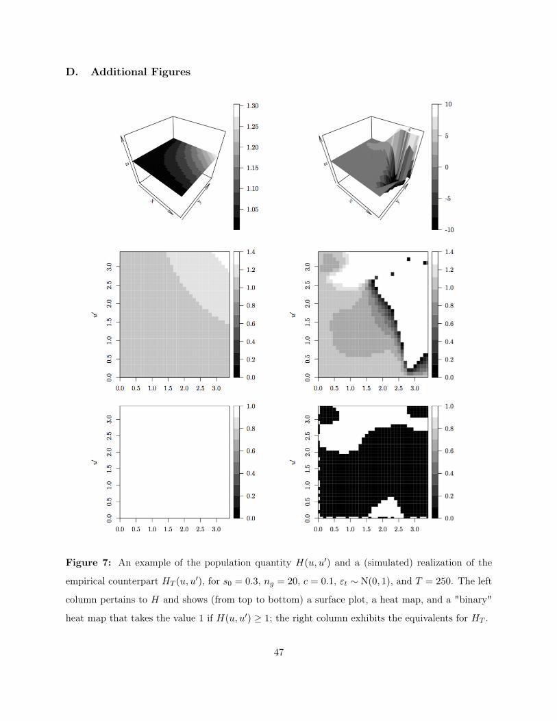
D. Additional Figures

Figure 7: An example of the population quantity H(u, u′) and a (simulated) realization of the

empirical counterpart HT (u, u′), for s0 = 0.3, ng = 20, c = 0.1, εt ∼ N(0, 1), and T = 250. The left

column pertains to H and shows (from top to bottom) a surface plot, a heat map, and a "binary"

heat map that takes the value 1 if H(u, u′) ≥ 1; the right column exhibits the equivalents for HT .

47

Figure

8:Truec.f.ϕ

∆P

andtw

ocorrespo

ndinge.c.f.’sϕT

=250an

dϕT

=5000,alon

gwiththecorrespo

ndingap

proxim

ationerrors.

The

real

and

imag

inarypa

rtofϕT

=250an

dϕT

=5000in

theleft

plot

areprojected

onto

therespective

plan

es.

The

e.c.f.’sare

compu

tedfrom

asimulated

sampleof

leng

thT

=5,

000withs 0

=0.

3an

dε t∼

N(0,1

),whereϕT

=250is

compu

tedfrom

thefirst

250elem

ents

ofthesample.

48

References

Aczel, J. (1966). Lectures on Functional Equations and Their Applications. Academic Press, New

York.

Andersen, T. G. and Bondarenko, O. (2014). Vpin and the flash crash. Journal of Financial Markets,

17:1–46.

Angel, J. J., Harris, L. E., and Spatt, C. S. (2011). Equity trading in the 21st century. The Quarterly

Journal of Finance, 1(01):1–53.

Bisgaard, T. M. and Sasvári, Z. (2000). Characteristic Functions and Moment Sequences: Positive

Definiteness in Probability. Nova Publishers.

Bleaney, M. and Li, Z. (2015). The performance of estimators of the bid-ask spread under less than

ideal conditions. Studies in Economics and Finance, 32:98 – 127.

Bradley, R. C. (2005). Basic properties of strong mixing conditions. a survey and some open

questions. Probability Surveys, 2:107–144.

Carrasco, M., Chernov, M., Florens, J.-P., and Ghysels, E. (2007). Efficient estimation of general

dynamic models with a continuum of moment conditions. Journal of Econometrics, 140(2):529–

573.

Carroll, R., Ruppert, D., Stefanski, L., and Crainiceanu, C. (2006). Measurement error in nonlinear

models. Chapman and Hall.

Castura, J., Litzenberger, R., Gorelick, R., and Dwivedi, Y. (2010). Market efficiency and mi-

crostructure evolution in us equity markets: A high-frequency perspective. Russell: The Journal

Of The Bertrand Russell Archives, 24.

Corwin, S. and Schultz, P. (2012). A simple way to estimate bid-ask spreads from daily high and

low prices. Journal of Finance, 67:719 – 760.

Cox, D. R. (1972). Regression models and life-tables. Journal of the Royal Statistical Society. Series

B (Methodological), pages 187–220.

49

Easley, D., de Prado, M. M. L., and O’Hara, M. (2012). Flow toxicity and liquidity in a high-

frequency world. Review of Financial Studies, page hhs053.

Feuerverger, A. (1990). An efficiency result for the empirical characteristic function in stationary

time-series models. Canadian Journal of Statistics, 18(2):155–161.

Foucault, T., Pagano, M., and Roell, A. (2013). Market Liquidity: Theory, Evidence and Policy.

Oxford University Press.

Gassiat, E. and Rousseau, J. (2016). Nonparametric finite translation hidden markov models and

extensions. Bernoulli, 22:193 – 212.

Goyenko, R., Holden, C., and Trzcinka, C. (2009). Do liquidity measures measure liquidity? Journal

of Financial Economics, 92:153 – 181.

Harris, L. (1990). Statistical properties of the Roll serial covariance bid/ask spread estimator. The

Journal of Finance, 45(2):579–590.

Hasbrouck, J. (2004). Liquidity in the futures pits: Inferring market dynamics from incomplete

data. Journal of Financial and Quantitative Analysis, 39(02):305–326.

Hasbrouck, J. (2009). Trading costs and returns for us equities: Estimating effective costs from

daily data. The Journal of Finance, 64(3):1445–1477.

Hu, Y. (2016). Microeconomic models with latent variables: Applications of measurement error

models in empirical industrial organization and labor economics. Journal of Econometrics, forth-

coming.

Jones, C. M. (2002). A century of stock market liquidity and trading costs. Available at SSRN

313681.

Kirilenko, A. A., Kyle, A. S., Samadi, M., and Tuzun, T. (2014). The flash crash: The impact of

high frequency trading on an electronic market. Available at SSRN 1686004.

Lukacs, E. (1972). A survey of the theory of characteristic functions. Advances in Applied Probability,

4(1):1–38.

50

Newey, W. and McFadden, D. (1994). Handbook of Econometrics, volume IV, chapter 36 Large

Sample Estimation and Hypothesis Testing. Elsevier.

Roll, R. (1984). A simple implicit measure of the effective bid-ask spread in an efficient market.

The Journal of Finance, 39(4):1127–1139.

Stein, E. and Shakarchi, R. (2003). Complex Analysis. Princeton, NJ: Princeton University Press.

U.S. SEC & U.S. CFTC (2010). Findings regarding the market events of May 6, 2010 (Report of the

Staffs of the CFTC and SEC to the Joint Advisory Committee on Emerging Regulatory Issues).

Ushakov, N. G. (1999). Selected topics in characteristic functions. Walter de Gruyter.

Zhang, H. and Hodges, S. (2012). An extended model of effective bid-ask spread.

51