simple maths for scientists

8/14/2019 Simple Maths For Scientists

http://slidepdf.com/reader/full/simple-maths-for-scientists 1/33

SIMPLE MATHEMATICS

FOR SCIENCE

John L Bähr & John N DoddDepartment of Physics

University of Otago2002



Simple Maths for Science

Physics Department, University of Otago

1 PHYSICAL QUANTITIES 3

2 MATHEMATICAL EQUATIONS - STATEMENT OF A PHYSICAL RELATION 3

2.1 NOTATION 5

3 BUILDING AN EQUATION AND READING SENSE INTO IT 5

4 MATHEMATICAL EQUATIONS 8

Range of validity of an equation. 8

5 SCIENTIFIC NOTATION AND SIGNIFICANT FIGURES 9

6 SIMPLE MANIPULATION OF SIMPLE EQUATIONS 10

Rule I 11

Rule II 11

7 SIMPLE EQUATIONS, SOLUTIONS AND GRAPHS 12

7 .1 The PROPORTIONAL relationship. 12

7.2 The LINEAR relationship. 14

7 .3 The QUADRATIC relationship 16

7.4 The INVERSE relationships 17

8 THE GEOMETRY OF THE CIRCLE AND THE SPHERE 18

9 THE GEOMETRY OF A TRIANGLE 20

10 SIMPLE TRIGONOMETRY 23

10.1 The SINE and COSINE function of an angle 23

10.2 Angles greater than 90 o

25

11 RATES OF CHANGE 26

12 EXPONENTIAL BEHAVIOUR 28

12.1 EXPONENT notation 28

12.2 The EXPONENTIAL function 28

13 THE LOGARITHM AND THE LOGARITHMIC FUNCTION 32

13.1 LOGARITHMIC SCALE 32

13.2 The DECIBEL 33

• Note: Answers to the exercises are available from the Physics Department





SIMPLE MATHEMATICS FOR SCIENCE

1 PHYSICAL QUANTITIES

Physical quantities such as distance, time, temperature, current , etc. are measured by a number and

a unit :

distance x = 5 m

∂ = 3.6 km

time t = 125 s

T = 5.0 µs

temperature T = 20o

C

= 293 K

These are examples of scalar quantities (a number and a unit only). Sometimes a statement of

direction in space is needed also - vector quantities

displacement x = 5 m to the right

y = 12 m upward

velocity v = 0.7 ms-1

to NE

force F = 19.6 N downward.

A vector physical quantity is sometimes denoted by → over its symbol, and this is the most graphic

way to represent it in manuscript; in print it is usually denoted ( as above ) by bold type.

Area is also really a vector quantity but we will not treat it as such. The area of a 20c piece [6.16 x

10-4

m2 ] has a different orientation in space if it is lying on a table than if it is on edge:

Pressure ( = force per unit area ) is a scalar

P = 160 Nm-2

= 160 Pa

Care must be taken when dealing with vector quantities. We shall discuss simple cases later, but

for now will discuss only scalar physical quantities.

2 MATHEMATICAL EQUATIONS - STATEMENT OF A PHYSICAL RELATION

You will note above that we have used algebraic symbols (usually roman or greek letters) to stand

for physical quantities: we have introduced x , ∂, y to stand for distances and displacements. In





science these are always measured in metres (symbol m) so that a statement about where something

is (measured from some reference point origin) is made by giving a number and the unit. Thus the

symbolic statement

x = 5 m (to the right)

can be read as

"The displacement of an object is five metres to the right of the origin".

If the direction of the displacement is not important, ie if we only want information about how far

the object is from the origin, we can dispense with the vector symbolism and language and write

x = 5 m, or

"The displacement of the object is 5 m from the origin".

Note that the mathematical equation:

x = 5 cm,

or in general x = a

(where a is any distance), is just a sentence.

The quantity on the LHS ( here x ) is the subject of the sentence. The = sign is the verb (other

verbs are ≠, >, <, >>, << etc) . The quantity on the RHS is the object of the sentence. Being a

sentence, a mathematical equation is subject to the rules of grammar and syntax which go to make

sensible language. The quantities on the two sides of an = sign must be the same type of

physical quantity. For example, in sensible ordinary language, you can’t say

"2 horses equal 200 dollars" ,

[on substituting a different verb - eg "cost" rather than "equal" the statement may make sense].

One can say

"2 dollars equal 200 cents",

because the dollar and the cent are both quantities of the same thing - money.

In science, we try to use the same unit all the time. In the above case we could adopt the dollar as

the standard unit and we should then have to write

"2 dollars = 2 dollars".

The number and the unit must agree on both sides of the equation.

Note however that it is permissible to use decimal multipliers for the units ( they are the equivalent

of adjectives ):

1 km = 1000 m

2.73 x 10-5

m = 27.3 µm= 2.73 x 10-2 mm

= 0.0273 mm.

Learn the use of the following multipliers:





G = giga = 109

M = mega = 106

k = kilo = 103

m = milli = 10-3

µ = micro = 10-6

n = nano = 10-9

p = pico = 10-12

There are others which may be introduced from time to time. Note the necessity of distinguishingthe use of upper case symbols ( eg M for mega ) and lower case symbols ( eg m for milli ).

Newspapers often fail to recognise the important distinction; a statement that the output of a powerstation is 150 mW is usually quite alarming news.

2.1 NOTATION

In text and printed material a physical quantity is normally written in italic font . This practice is

not followed in manuscript, so, in your written work, you must be quite careful not to confuse

physical quantities and units.

The unit (and any multiplier used with it) is written in plain upright font.If a unit is called after a person, that unit, when spelt in full, is written with a small letter ( newton,

amp, volt, watt); but the symbol for that quantity always reverts to the capital ( N, A, V, W ).

Examples

F = 9.8 N ↓, reads "the (vector) force is 9.8 newtons downwards";

I = 10 µA, reads "the electric current is ten micro-amps";V = 230 V, reads "the voltage (or potential, or potential difference) is 230 volts;P = 1.2 kW, reads "the power is 1.2 kilo-watts".

3 BUILDING AN EQUATION AND READING SENSE INTO IT

Suppose we wish to describe where an object is at various instants of time. The object is movingalong a straight line (which we may call the x-axis) and we measure all distances from a fixed pointor origin (0) on that line. Positions to the right of the origin will be called positive and those to the

left of the origin will be negative.

-2 0 +2 +4 +6 +8 +10

t = 0x /m

We are going to let x stand for the distance an object is from the origin at time t .

[Note the use of x /m to label the axis:

x stands for a physical quantity, distance, which is measured as "so many metres". Being aphysical quantity it is written in italics. Dividing by "metres" (as implied by /m) means we are

left with a pure number; these are the numbers used to label the axis. We label the line with a setof numbers representing the number of metres from the origin.]

Example: Let the object be at position x0 at t = 0.

Example 1: Let the object be 2 m to the right of the origin at t = 0: x0 = 2 m.

If it remains stationary ( velocity is zero, v = 0 ), it remains always at the same position, the initialposition. Therefore the equation of motion is a trivial:





(3.1) x = x0 = 2m.

Example 2: The object is moving to the right with a constant velocity of 1.5 ms-1.The velocity at t = 0 is

v0 = 1.5 ms-1,

the subscript 0 being used to indicate the value of v at time zero. Since the velocity remainsconstant with time,

(3.2) v = v0 = 1.5 ms-1

During a time interval t an object moving at a constant velocity v‚ has moved a distance = velocity

x time [ eg: When driving at 65 km/hr for two hours, we move a distance of 65 km/hr x 2 hr = 130km. When speeding at 1000 ms-1 for a time interval of 2 ms, ( note the meanings "metre persecond" and "millisecond" respectively), a rocket travels

1000 ms

-1

x 2 ms = 1000 ms

-1

x 0.002 s = 2 m.It is wise, while building up your confidence at using equations and making mathematicalstatements with physical quantities, to be quite pedantic in writing numbers and units. When you

get a bit more experience a few short cuts can be taken ].

Therefore, if an object moves at a constant velocity v0 for a time interval t, it moves a distance

x = v0 x t .This is frequently written more simply as x = v0t ; ( when two or more symbols for physicalquantities are placed next to each other this means that they are multiplied together ). Note that as

well as the numbers being multiplied, so are the units:

distancemetressecondsecond

metres

(time)(velocity) →=→ This distance moved in a time interval t is sometimes referred to as an increment of displacement

or position, and is symbolized by ∆ x (read as "delta x"):

(3.3) ∆ x = v0t .

The final position of the moving object = the initial position + the increment of position:

x = x0 + ∆ x(3.4) x = x0 + v0t

This is called an EQUATION OF MOTION; it is an equation that tells where the object is ( x ) at

a certain instant of time (t ). The quantities x0 ‚ and v0 ‚ are called the initial conditions, i.e. theposition and speed of the object at time zero. In this case it is the equation of motion for an object

that is moving at constant velocity (constant speed along a straight line ). We shall find otherequations of motion for other circumstances.

The great advantage of this mathematical expression is its generality. Thus, using (3.4) , for

x0 = +2 m and v0 = +1.5 ms-1 :

at t = 0, x = x0 = 2 m;at t = 1 s, x = x0 + v0 x (1 s) = 2 m + (1.5 ms-1)(1 s) = 3.5 m;

at t = 2 s, x = 2 m + (1.5 ms-1)(2 s) = 5 m;





at t = 3 s, x = 2 m + (1.5 ms-1)(3 s) = 6.5 m;

at t = 206 s, x = 2 m + (1.5 ms-1)(206s) = 311 m;at t = -5 s, x = 2 m + (1.5 ms-1)(-5 s) = -5.5 m.

One equation expresses the conditions for all times; and the same equation is used for differentinitial conditions.

Exercises: Work out for the times in the above example the position for the following initial

conditions:

Ex(1) x0 = 0, v0 = 2 x 104 ms-1

Ex(2) x0 = 10 m, v0 = - 0.2 ms-1

Example 3: As a further example of building up a useful equation we shall consider the case of anobject moving along a line with acceleration; i.e. the velocity does not remain constant as in (3.2)

above. We write

(3.5) v = v0 + at ,

where a is the acceleration, eg if at t = 0, v0 = 1.5 ms-1 and a = 0.4 ms-2, then the velocities at

later instants are:

at t = 0 v = v0 = 1.5 ms-1 at t = 1 s v = 1.5 + 0.4 x 1 = 1.9 ms-1

at t = 2 s v = 1.5 + 0.4 x 2 = 2.3 ms-1 at t = 3 s v = 1.5 + 0.4 x 3 = 2.7 ms-1

i.e. in each successive second the velocity has increased by an increment of 0.4 ms-1 . We say"there is an acceleration of 0.4 metres per second, per second" , or a = 0.4 ms-2 .

What is the equation of motion, i.e. an equation relating x and t , for this case where there is

acceleration? There are now two contributions to the increment of displacement. The first we havealready discussed; (3.3) gives for the increment in time t caused by the (initial) velocity v0:

(∆ x )v = v0t .

There is a further increment due to the fact that the object is accelerating, because the velocity

during the time from t = 0 to t when the motion is taking place is not always v0, but is increasingaccording to (3.5). We shall show later that the increment in distance x caused by non-zero

acceleration is :

(∆ x )a = (1/2) x acceleration x the square of the time, or

(3.6) (∆ x )a = a t 2 /2, [ note that this term is zero if a = 0 ].

The final position of the object at time t is: the initial position ( x0 ) plus the increment due to

initial velocity (v0t ) plus the increment due to acceleration ( at 2 /2 ) :

x = x0 + (∆ x )v + (∆ x )a





(3.7) x = x0 + v0t + at 2 /2 .

This is the EQUATION OF MOTION of an object moving along a straight line with constant

acceleration. Note that if a = 0 the equation reduces to that in (3.4), and that if v0 = 0 , it

reduces to (3.1).

Exercises:Ex(3) Using x0 = 2m, v0 = 1.5 ms-1, and a = 0.4 ms-2, calculate x at t = -5 s, 1 s, 2 s, 206 s.

Ex(4) Calculate again, using a = - 0.4 ms-2. What does this negative acceleration mean?

4 MATHEMATICAL EQUATIONS

Some time has been spent in the previous section showing how a mathematical equation is built up

to represent some scientific statement - a statement which can be made of a quantitative nature. The

advantage of the mathematical equation is its conciseness - the equations used in physics, or

indeed in any science, should not be thought of so much as mathematics but as a concise and

precise way of writing a scientific statement .

For much of science, and certainly for beginning courses in physics, the level of mathematicsneeded to express scientific statements, and to make predictions from them, is quite simple. Themain problem is to recognise and to understand the scientific principle involved, and to translate

that into mathematical language. Once that has been done the mathematical processing usuallyproceeds quite easily. The further problem exists in translating the mathematical answer back intoscientific predictions. It is for this reason that we have above spent some time on building up and

interpreting an equation. Later we shall study some other types of equation.

Range of validity of an equation.

In the example above, we have discussed the equation of motion of an object that has position x0

and velocity v0 at the instant t = 0, and moves with constant acceleration a . We found twoequations which give the displacement and velocity of the object at any later time t .

x = x0 + v0t + at 2 /2 ( 3.7)

v = v0 + at . ( 3.5) .

Two questions can immediately be asked:

Is it really only for later times; what about earlier times, i.e. before t = 0, for which t would be a

negative number of seconds ? Are the equations valid for all times ?

The answer to the first question is that the equation is certainly usable for earlier (negative) times:this has been done in one of the examples worked out earlier. The presumption would then be that

the object has been moving in such a way that it reaches the initial condition ( in this case x0 =

2m, v0 = 1.5 ms-1) at the initial time ( in this case t = 0 ). On the other hand, it could perhaps havebeen that the object had remained at rest at the position x0 = 2 m at times earlier than t = 0 andthen, at that instant, was given a velocity v0 = 1.5 ms-1 together with an acceleration of a = 0.4 ms-

2 to further increase the velocity. In this case the range of validity of the equation is only for times

after t = 0. Prior to this the object would have remained stationary at x = x0 = 2m; thus (3.1)would apply for t < 0, whereas (3.5) and (3.7) would apply for t > 0.The answer to the second question is more subtle. If the equations of motion are valid for all times

then, for example, (3.5):

v = v0 + at





means that, after 25 years = 25 x 365.25 days

= 25 x 365.25 x 24 hours= 25 x 365.25 x 24 x 60 minutes= 25 x 365.25 x 24 x 60 x 60 seconds

= 788 940 000 s,the velocity will reach

v = 2 ms-1 + 0.4 ms-2 x 788 940 000 s= 315 576 002 ms-1 ??

Now this enormous speed is, in fact, faster than the speed of light, and we know through the

theory of relativity that it is impossible to accelerate something to greater than the speed of light(299 792 458 ms-1). We must therefore conclude that the equations of motion that we have

deduced are valid only for the range of nonrelativistic velocities ( i.e. velocities that are much lessthan the speed of light).

In a similar way all other equations which represent a scientific statement may have limited ranges

of validity.

5 SCIENTIFIC NOTATION AND SIGNIFICANT FIGURES

In the above numerical example numbers have been calculated to nine figures. First of all this isclumsy and makes it difficult to appreciate the size of quantities. Secondly, the statement of ninefigures implies an accuracy of measurement or of knowledge that is well beyond the normal

experiment.

(i) Scientific or exponential notation: Using powers of 10 :

100 = 10 x 10 = 102

1 000 = 10 x 10 x 10 = 103

1 000 000 = 106

1 000 000 000 = 109 etc.Furthermore

3

2

1

101000

1

10100

1

1010

1

−

−

−

=

=

=

Using this scientific notation, the velocity v = 315 576 002 ms-1 would be written:

v = 3.155 760 02 x 108 ms-1 .

We can immediately appreciate that this is larger than the velocity of light in vacuum:

c = 2.997 924 58 x 108 ms-1,

and therefore is a velocity that is unattainable according to Einstein’s theory of relativity.

Likewise for small quantities: the mass of a proton should not be written as

mp = 0.000 000 000 000 000 000 000 000 001 672 613 kilogram (kg).Rather this should be written as





mp = 1.672 613 x 10-27 kg .

This is not only tidier, but it gives more immediately a concept of the order of magnitude of thequantity ( here, 10-27 kg ).

(ii) The accuracy to which we quote a numerical quantity. In the examples of velocities

quoted above we have used nine significant figures. Now, there are some cases of extremelyaccurate experiments, when we may indeed need to know a quantity to such fine precision (it is

defined that the velocity of light is 299 792 458 ms-1); but in many cases much less precision isneeded. For most purposes to quote the velocity of light in vacuum as

c = 3.00 x 108 ms-1

is quite precise enough ( it is within 1 part in 300 of the accurate result ). And the velocity of the

object given above as 3.155 760 02 x 108 ms-1 ( if such a velocity were possible ) would much moresensibly be written as

v = 3.156 x 108 ms-1 ,

if the accuracy were of the order of 1 part in 3000. Indeed we may often quote a quantity only to

within 10% say, in which case we would write

v = 3.2 x 108 ms-1 .

Learn to express measurements of scientific quantities in scientific notation, and with a number of significant digits appropriate to the sort of accuracy implied in the problem.

6 SIMPLE MANIPULATION OF SIMPLE EQUATIONSWe often need to manipulate an equation to bring a certain quantity into isolation - say on to theleft hand side of the equation.

We shall start by studying the form of mathematical equations. We shall restrict our discussion to

equations which relate two quantities to each other. We shall use x and y ( above we used x and t

representing displacement and time, but x and y may be any quantities which are somehow relatedby some process ). An equation of the sort

(6.1) y = x + f

has two TERMS on the right-hand side, x and f ; terms are added or subtracted. The equation

(6.2)m

xgxd y

2

+=−

has two terms on each side. But now each of the terms on the right hand side has several

FACTORS:

gx has two factors, g and x

x

m

2

has three factors, x times x divided by m , or x times x times (1/ m ) .

The equation(6.3) y = px





has two FACTORS on the right hand side, p times x ; factors are multiplied or divided.

(6.4) y = x/m

also has two factors on the right hand side, x times (1/ m ) or x divided by m .

Rule I A term in an equation can be transferred from one side to the other by changing its sign.

Examples:(i) (6.1) can be written y - f = x .

(ii) (6.1) can also be written in three other ways:

f y x

f y x

f x y

−=−

=+−=−−

0

0

(iii) (6.2) can be written y = d + gx + x2 / m.

Rule II

A factor in an equation can be transferred from one side to the other by moving it from thenumerator to the denominator (or vice versa).

(iv) (6.3) can be written x = y / p ,

(v) (6.4) can be written x/y = m , etc.

When the equations are more complicated containing terms each with factors as in (6.2), or in

equations like

(6.5) p ( y - f ) = ( x + g)( x - h)

where each side consists of two factors and three of these, ( y - f ), ( x + g) and ( x - h) contain twoterms each, more care is needed.

(vi) (6.2), after being rewritten as in (iii), can be multiplied through by m to give

x 2 + mgx + md = my .

(vii) (6.5) can be rewritten as

( )( )

p

h xg x f y

−+=−

or

( )( ) f

p

h xg x y +

−+=

thereby obtaining a form in which y stands alone on the left hand side - this is called SOLVING for y .





Exercises:

Ex(5) From (6.1) solve for f .Ex(6) From (6.2) solve for d .

Ex(7) From (6.2) solve for g .Ex(8) From (6.3) solve for p .

Ex(9) From (6.4) solve for x .Ex(10) From (6.5) solve for g .Ex(11) From (6.5) solve for h .

If you try to solve (6.2) or (6.5) for x you will encounter difficulties because you cannot easily place

x alone on the left hand side without it appearing elsewhere. This is because the equations containan x

2 term as well as an x term. The best one can do initially is to reduce the equation to the

QUADRATIC form:

(6.6) ax 2 + bx + c = 0

where a, b, c are each some combination of the other quantities that appear in the originalequations.

Exercises:

Ex(12) Reduce (6.2) to this form, and express a, b, c in terms of d, g, m, y.

Ex(13) Reduce (6.5) to this form, and express a, b, c in terms of p, y, f, g, h .

[ Additional note: the solution of the quadratic equation (6.6) is well-known but we shall not use it.We quote it here simply for reference purposes. There are two values for x (or sometimes none) forwhich the equation is true

a

acbb x

2

42 −±−= ]

If you have always found mathematics difficult or confusing, you have perhaps struggled in the lastsection. It has in fact gone slightly past the level of algebraic complexity needed for simple science.Try to achieve competency in the above and you should be able to handle any algebraic

manipulation required. We shall now return to simpler equations met with in simple physics.

7 SIMPLE EQUATIONS, SOLUTIONS AND GRAPHS

7.1 The PROPORTIONAL relationship.

The simplest equation is the PROPORTIONAL relationship between two physical quantities

represented by x and y :

y is proportional to x

meaning that, for example, if we halve the value of x then we halve the value of y , or if we treble

x then we treble y . Such is the behaviour in many scientific situations. We write

y ∝ x

[ the symbol ∝ , meaning "proportional to", is another mathematical verb ].

This may also be written as an equation:





(7.1) y = kx

where k is a constant quantity, independent of the values of x and y . The quantity k is called the

constant of proportionality. An example of this proportional relationship:

y may stand for the pressure exerted by a gas on the walls of an enclosure of constant volume, and x

may be the temperature of the gas. In this case (7.1) would probably be written as

(7.2) p = kT ,

using symbols which more closely indicate the meaning of the relationship. The equation is astatement of the well-known observation ( called Charles’s Law ) that the pressure of a gas is

proportional to the temperature.(It is assumed that the volume of the gas is kept constant while any temperature change takes place.It is known that the pressure also changes as the volume V is expanded or contracted. Thus we

anticipate a more complicated equation involving three quantities p, V, T . We restrict ourselvesmeanwhile to the simple case.)

Example:Take 0.004 kg of helium gas (this is 1 mole of helium). Place it in a constant volume enclosure of volume 10-3 m3 (this is 1 litre). The pressure exerted on the walls is:

(7.3) p = ( 8300 Pa K-1 )T

( the constant of proportionality, k = 8300 Pa K-1, has been rounded to two significant digits ).The constant must have units of pascal (Pa) per degree kelvin (K) because, when it is multiplied bya temperature measured in degrees kelvin, the answer must be in the standard unit of pressure

(newton per square metre = Nm-1 = pascal = Pa). The equation is often more simply written as p

= 8300 T but, strictly speaking, the constant is not the number 8300 but is the physical quantity8300 Pa K-1.

Thus, when the temperature, T , is 293 K ( = 20o celsius ), the pressure is

p = 2.43 x 106 Pa

p = 2.43 MPa.

[ How big is this? Well, the pressure of the atmosphere at the surface of the earth is 1.01 x 105 Pa.

So the pressure of helium in the above container is about 24 atmospheres ].

It is often very useful and instructive to illustrate physical behaviour by the use of graphs. In thiscase, representing proportional behaviour, the graph is a STRAIGHT LINE THROUGH THEORIGIN (T =0, p=0).

The graph, which represents the behaviour of a gas, is a straight line; at very low temperatures andat very high temperatures (7.2) or (7.3) may run outside their range of validity. At very lowtemperatures the gas may condense to a liquid; at very high temperatures other things may occur.

In the case of helium the equation fairly represents the behaviour from somewhere below 10 K tomany thousands of degrees.





0.0

0.5

1.0

1.5

2.0

2.5

3.0

3.5

4.0

4.5

0 200 400 600T/K

p / M P

a

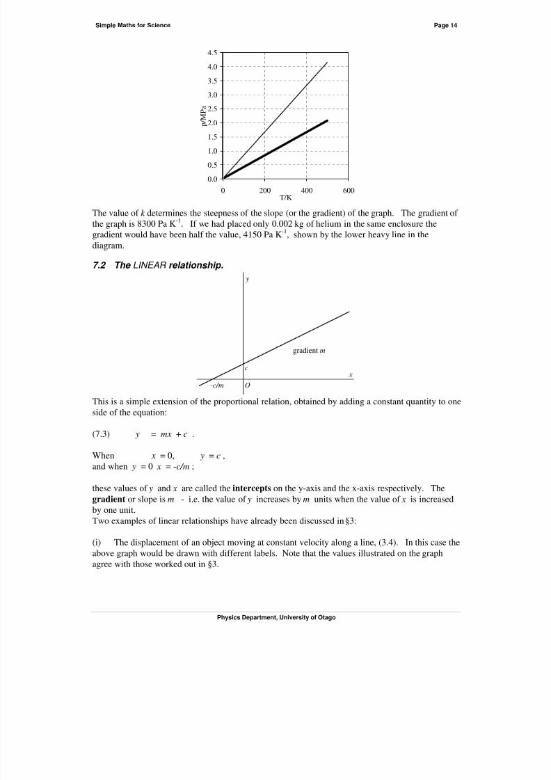
The value of k determines the steepness of the slope (or the gradient) of the graph. The gradient of

the graph is 8300 Pa K-1

. If we had placed only 0.002 kg of helium in the same enclosure thegradient would have been half the value, 4150 Pa K -1, shown by the lower heavy line in the

diagram.

7.2 The LINEAR relationship.

c

O-c/m

gradient m

y

x

This is a simple extension of the proportional relation, obtained by adding a constant quantity to one

side of the equation:

(7.3) y = mx + c .

When x = 0, y = c ,and when y = 0 x = -c/m ;

these values of y and x are called the intercepts on the y-axis and the x-axis respectively. The

gradient or slope is m - i.e. the value of y increases by m units when the value of x is increasedby one unit.

Two examples of linear relationships have already been discussed in §3:

(i) The displacement of an object moving at constant velocity along a line, (3.4). In this case the

above graph would be drawn with different labels. Note that the values illustrated on the graph

agree with those worked out in §3.





-2

-1

0

1

2

34

5

6

7

8

9

-4 -2 0 2 4 6t /s

x /m

(3.4) x = x0 + v0t

(ii) The velocity of an object moving with constant acceleration along a straight line, (3.5).

(3.5) v = v0 + at

0

0.5

1

1.5

2

2.5

3

3.5

-2 0 2 4 6

t /s

v /ms-1

Exercises:

Using the graph and/or the equation for motion with constant velocity along a line, with x0 = 2m,

v0 = 1.5 ms-1, calculate:

Ex(14): where the object will be at t = 4 s?Ex(15): when the object passed the origin?

Using the equations ( 3.5 and 3.7) for motion with constant acceleration,

with x0 = 1.8 m, v0 = 1.5 ms-1, a = 0.4 ms

-2, calculate:

Ex(16): the velocity of the object at t = 5 s.Ex(17): the position of the object at t = 5 s.Ex(18): at what time was the velocity zero?

Ex(19): at what time was the object at x = 0? ( This requires the solution of a quadraticequation as given in §6. Try it for fun ).





7.3 The QUADRATIC relationship

We have met this before in (3.7), the equation of motion of an object with constant acceleration

along a line. To simplify matters we consider the case where the object starts at the origin ( x0 = 0)with zero velocity (v0 = 0). The general quadratic equation of motion then reduces to:

(7.4) x = at 2 /2 and v = at .

02

4

6

8

10

12

14

16

18

-4 -2 0 2 4 6

t /s

x /m

0

0.2

0.4

0.6

0.8

1

1.2

-2 -1 0 1 2 3 4

t /s

v /ms-1

The graph of x against t is no longer a straight line. The gradient which, as was shown in a

previous example, represents the velocity of the object, increases with time; thus the gradient gets

steeper and steeper as time goes on. Also plotted is velocity versus time for this case when v0 = 0.

Exercises:

Ex(20) Check the values of x and v at t = 0, 1, 2, 3 s , using a = 0.4 ms-2.Ex(21) What are the values of x and v for t = -1, -2 s?

The curve of x vs t is called a PARABOLA. It is one of a number of second order curves (when

there is a squared term in the equation). Other second order ( or conic section ) curves are the ellipse

(and its special case, the circle) and the hyperbola. These curves are the paths in space of planets,satellites and comets.





0

1

2

3

4

5

6

7

0 5 10 15 20

t 2 /s

2

x /m

It is often useful in science to plot a curve in such a way as to make it a straight line - then one can

check more easily whether there are errors. In the present case this can be done by plotting x

against t 2, rather than against t .

7.4 The INVERSE relationships The inverse relationship is where one physical quantity (say y) is proportional to the reciprocal of

the other (say x ) :

y ∝ 1/ x

therefore

(7.5) y = k / x

In this case, as x gets larger y gets smaller, and vice versa, in such a way as to keep the product of xand y constant:

(7.6) xy = k .

An example in physics comes again from the properties of a gas. This time the gas is contained in

an enclosure whose volume V can be altered. If the temperature is kept constant the pressure, p ,exerted on the walls by the gas varies inversely as the volume, according to the relationship:

p ∝1/ V ,

or

(7.7) pV = constant.

0

1

2

3

4

5

6

0 1 2 3

V/10-3

m3

p/MPa





This is known as Boyle's law. It is this law, when combined with that discussed in §7.1, that leads

to the universal gas equation:

(7.8) pV = nRT .

n is a measure of the amount of gas used and R is a universal physical constant.

A graph is shown above. Note how the marked point on the graph agrees with the calculationspreviously made; the graph therefore corresponds to the behaviour of the chosen amount of gas

(0.004 kg of helium) at the chosen temperature (293 K = 20oC). This curve is called a

HYPERBOLA.

The graph could be drawn as linear if, instead of plotting p against V , we plotted p against 1/ V .

0

2

4

6

8

10

12

0 1000 2000 3000 4000

(1/V)/m-3

p/MPa

In the above discussion we have introduced the simplest mathematical relationships - calledmathematical functions - linear and quadratic and inverse. There are three others which we shall

need:

the sine (or cosine) function that occurs in vibration and waves

the exponential function that occurs in growth and decay

the logarithmic function that is used in graphical scales and for certain measurements in sound (thedecibel ).

We postpone discussion of these until we have studied the GEOMETRY of two important shapes:

• the circle ( and the related sphere ) and

• the triangle.

8 THE GEOMETRY OF THE CIRCLE AND THE SPHERE

Consider a circle of radius = r

(8.1) diameter = d = 2r

(8.2) circumference = 2πr = πd

(8.3) area = πr 2





The symbol π (the Greek letter pi) stands for a certain irrational number (i.e. one which, when

expressed as a decimal, goes on for ever without repeating itself and can never be expressed with

complete accuracy by any ratio of two integers - although π = 22/7 is a pretty good approximation).

From one of the above relations you can see that π is the ratio of the length of the circumference to

the diameter of a circle. The value of π has been calculated, by enthusiasts for this sort of thing, to

an enormous number of places. For our purposes

π = 3.1416 ..........

= 3.14 ........= 3 ....... depending on how accurate one needs to be.

diameter

angle

radius = r arc

circle

circumference = 2πr area = πr

2

sphere

surface area = πd 2

diameter = d

volume = πd 3 /6

ANGLE: there are three different ways of measuring angle -

(i) in revolutions,(ii) in degrees,(iii) in radians, ( the mathematician’s way) .

There are 360o of angle in 1 revolution. A right angle, made by two lines perpendicular to eachother, is 90o.

The radian is the angle at the centre of a circle when the arc is equal in length to the radius ( see the

above diagram ). One radian is close to 57.3o. One revolution = 360o = 2π radians.

Related to the two-dimensional figure of the circle is the three-dimensional object, the SPHERE:for a sphere of radius r

(8.4) the surface area = 4πr 2 = πd

2

(8.5) the volume = 4πr 3 /3 = πd

3 /6

Exercises:Ex(22) When a wheel of diameter 0.32 m rolls along a surface, how far does it travel in each

revolution?

Ex(23) A string is wound around the rim of a wheel of radius 0.2 m (below left):

(a) When the string has been pulled out by x = 0.1 m, how many degrees has thewheel turned?





b) How far must the string be pulled out to turn the wheel by 90o ?Ex(24) A wooden disk has the dimensions shown in the diagram (below right):

What is the area of the top face?

What is the area of the bottom face?What is the area of the curved face?

What is the total surface area?What is the radius of a sphere that has the same surface area?

x

axle 0.8m

0.25m

9 THE GEOMETRY OF A TRIANGLE

A

B

C

a

b

c

α

β

Join three points A, B and C, by straight lines, forming angles, α , β and γ .The length of the sides opposite these points or angles are a, b and c.

There are a number of relationships regarding lengths of sides, size of angles, and area for thegeneral triangle. We need to know only a few simple facts:

(i) The sum of the angles in a triangle equals 180o = 0.5 rev = π rad.

(9.1) α + β + γ = 180o = 0.5 rev = π rad ( for any triangle )

(ii) The angles of a triangle determine completely its shape. Two triangles drawn with thesame angles,

ie with the same shape, are called SIMILAR triangles; one is a scaled up version of the other; thesides are respectively proportional to each other





a

b

c a’

b’

c’ β

β

α

α

(9.2)cc

bb

aa ’’’ == ( for similar triangles )

(iii) A triangle with all three sides equal has all three angles equal. It is called an equilateral

triangle. Each angle is 60o or π /3 radian or 1/6 rev.

(iv) A triangle with one of its angles equal to 90o is called a right angled triangle ( note: anytriangle can always be split into two right angle triangles)

≡ a

b

c

90o

β

Because α + β + 90o = 180o

α + β = 90

o

(9.3) β = 90o - α ( for a right angled triangle )

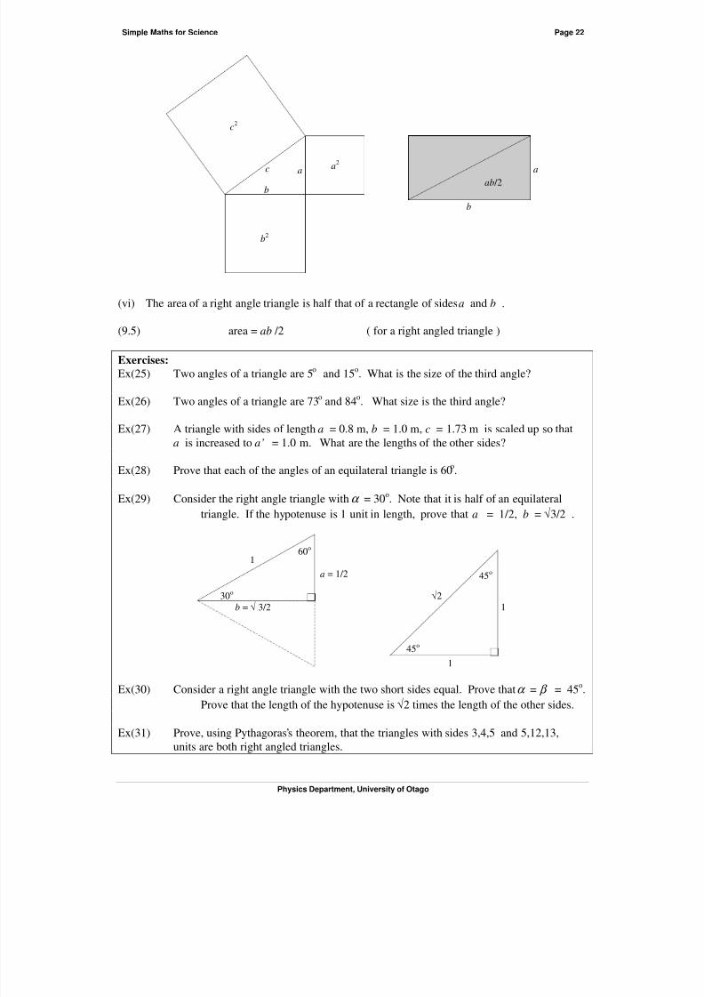
(v) Pythagoras (580 - 500 B.C.) proved, by pure geometrical reasoning, that the area of the square

on the longest side ( the hypotenuse, the side opposite the right angle ) is the sum of the areas of thesquares on the other two sides:

(9.4) a2 + b

2 = c2 ( for a right angled triangle )

[Note: this applies only to a right-angle triangle. If the angle γ between sides a and b is not a

right angle, the left hand side of this equation must be modified according to the size of the angle].





a

b

c

b2

a2

c2

a

b

ab /2

(vi) The area of a right angle triangle is half that of a rectangle of sides a and b .

(9.5) area = ab /2 ( for a right angled triangle )

Exercises:

Ex(25) Two angles of a triangle are 5o and 15o. What is the size of the third angle?

Ex(26) Two angles of a triangle are 73o and 84o. What size is the third angle?

Ex(27) A triangle with sides of length a = 0.8 m, b = 1.0 m, c = 1.73 m is scaled up so thata is increased to a’ = 1.0 m. What are the lengths of the other sides?

Ex(28) Prove that each of the angles of an equilateral triangle is 60o.

Ex(29) Consider the right angle triangle with α = 30o. Note that it is half of an equilateral

triangle. If the hypotenuse is 1 unit in length, prove that a = 1/2, b = √3/2 .

1

30o

60o

√2 1

1

45o

45

o

a = 1/2

b = √ 3/2

Ex(30) Consider a right angle triangle with the two short sides equal. Prove that α = β = 45o.

Prove that the length of the hypotenuse is √2 times the length of the other sides.

Ex(31) Prove, using Pythagoras’s theorem, that the triangles with sides 3,4,5 and 5,12,13,units are both right angled triangles.





10 SIMPLE TRIGONOMETRY

10.1 The SINE and COSINE function of an angle

θ N N’

P

P’

OP"

N"

An angle θ - measured in degrees or radians - is enclosed between two lines which intersect at a

point 0. From a point P on one line, draw a perpendicular (or normal ) to the other line, meetingit at point N. The angle at N is a right angle = 90o = π /2 radian. A second position P’N’is shown,

and also a third P"N" drawn with the positions of P and N reversed. But always, N is the rightangle.

By the properties of similar triangles, for any chosen position of P, the ratios of the sides are equal:

OP"

N"P"

OP’

N’P’

OP

PN==

The value of the ratio depends only on the size of the angle θ , and is independent of the chosenposition of P. We say "the ratio PN/OP is a function of the angle θ " . This function is called the

sine of the angle θ , and is written sinθ .

triangleanglerighttheof hypotenuse

triangleanglerighttheof sideopposite

OP

PNsin ==θ

Note: "opposite" side means that the side opposite to the angle being described; the"hypotenuse" is the side opposite the right angle, the longest side.

The variation of sinθ with angle θ is plotted in the diagram below. Note the following specialvalues of the sine of an angle:

sin(0o) = sin(0 rad) = 0

sin(30o) = sin(π /6 rad) = 0.5 = 1/2

sin(45o) = sin(π /4 rad) = 0.707... = 1/ √2

sin(60o) = sin(π /3 rad) = 0.866... =√3/2

sin(90o) = sin(π /2 rad) = 1.000

The variation of sinθ for angles outside the range 0o → 90o is discussed below.

Also, by the properties of similar triangles, the following ratios are also equal for any chosenposition of P:





OP"

ON"

OP’

ON’

OP

ON==

The value of this ratio also depends only on the size of the angle θ , and is independent of the

chosen position of P. We say "the ratio ON/OP is a function of the angle θ ". This function is

called the cosine of the angle θ , and is written as cosθ .

triangleanglerighttheof hypotenuse

triangleanglerighttheof sideadjacent

OP

ONcos ==θ

The variation of cosθ with angle θ is plotted in the diagram below. Note the following special

values of the cosine of an angle:

cos(0o) = cos(0 rad) = 1

cos(30

o

) = cos(π /6 rad) = 0.866... =√3/2cos(45o) = cos(π /4 rad) = 0.707... = 1/ √2

cos(60o) = cos(π /3 rad) = 0.5 = 1/2

cos(90o) = cos(π /2 rad) = 0 .

The variation of cosθ for angles outside the range 0o → 90o is discussed below.

There is a further ratio that is often used, the tangent of the angle:

θ

θ θ

cos

sin

ON

PN

sideadjacent

sideopposite=tan ==

Exercise:Ex(32) Check all the above quoted values for the sine and cosine of 0o, 30o, 45o, 60o, 90o

using the standard triangles drawn on page 18.

Ex(33) Using the graph of sine and cosine, or with the use of a calculator, find the angles inthe 3:4:5 and 5:12:13 triangles discussed above.

Ex(34) Using (9.3) prove that

(10.1) sin(90o - θ ) = cos θ

cos(90o - θ ) = sin θ

Ex(35) Using Pythagoras’s theorem prove that

(10.2) sin2θ + cos2θ = 1 .

[ sin2θ is the usual way of writing (sinθ )2 ].





The variations of sinT and cosT with angle T between 0o

and 90o

0

0.1

0.2

0.3

0.4

0.5

0.6

0.7

0.8

0.9

1

0 30 60 90Degrees

F u n c t i o n V a l u e

10.2 Angles greater than 90 o

y-axis

x-axis

M P

NO

r y

x

y

θ

The definitions of sine and cosine can be extended to more general angles through the followingarguments:

r

y

=== OP

OM

OP

PNsinθ

r

x==OP

ONcosθ

As θ increases and P goes around the circle, OP = r remains a positive quantity . But for 180o <

θ < 360o, P is in the bottom half of the diagram, y is negative and hence sinθ = y / r is negative.

For 90o < θ < 270o, P is in the left hand side of the diagram, x is negative and hence cosθ = x / r

is negative.





The values of sinTand cosTas P goes around two revolutions:

-1

-0.8

-0.6

-0.4

-0.2

0

0.2

0.4

0.6

0.8

1

-90 0 90 180 270 360 450 540 630 720Degrees

F u n c t i o n V

a l u e

It should be noted:

• That each curve repeats itself over each complete cycle ( 1 rev = 360o = 2π rad ).

• That the two curves have the same form, simply being displaced from each other by an angle(or phase) of 90o = 1/4 rev = π /2 rad.

Exercise: Ex(36) Give the values of cosθ and sinθ for the following angles:

135o, 260o, 300o, 405o, 840o.

11 RATES OF CHANGE

In the foregoing we have dealt with quantities which change with time.

For a moving object, its displacement from a given point changes with time. The rate of change of

displacement or position with time is called the velocity of the object. The velocity of an objectmay change with time. The rate of change of velocity is called the acceleration of the object.

We have also met situations where one physical quantity changes when another changes.

For a gas the pressure changes as the temperature is changed.For a gas the pressure changes as the volume is changed.

It is often necessary to know how much change (∆ y) takes place in one physical quantity ( y ) for a

given change (∆ x) in another one ( x). This is called finding the rate of change of y with x .

Consider a graph which represents the behaviour of two physical quantities x and y . Two points

(1 and 2) are marked where the changes in x and the corresponding changes in y are illustrated. If a

small change ∆ x about the point in question is accompanied by the corresponding change ∆ y , then

the gradient or slope of the curve is:

x y

x

y

withof changeof ratethe

curvetheof slopeorgradientthe

=∆∆

=

The two cases illustrated show:

as x increases then y increases: ∆ y is positive for ∆ x positive: the slope of the graph, ∆ y / ∆ x , is

positive: growth as x increases then y decreases: ∆ y is negative for ∆ x positive: the slope of the graph, ∆ y / ∆ x , is

negative: decay.





x

y

∆y

∆x

∆x

∆y

y2

y1

x1 x2

1

2

Obviously to get an accurate value for the gradient, or rate of change, at a point on the curve,

especially if the graph is highly curved ( i.e. the dependence of y on x is highly non-linear ), onemust make the calculation with ∆ x and ∆ y very small; otherwise all we get is an average gradient

or rate of change over finite changes in the physical quantities. Graphically, this is done by drawinga tangent to the curve at the point in question; the tangent has, by definition, the same gradient as at

the point on the curve. One then measures the gradient ∆ y / ∆ x of the tangent, as has already been

done in §7 on linear behaviour.

Mathematically, this process can be carried out by finding the limiting value of the ratio ∆ y/ ∆ x as

both ∆ x and ∆ y are made smaller and smaller, approaching zero. The mathematical process by

which this is carried out is called the differential calculus. We shall not be using this branch of

mathematics but you should recognise the notation and understand its meaning.

The rate of change of y with x

x

y

x

y

∆∆

== of limitthed

das both of the increments ∆ x and ∆ y tend to zero.

∆x

∆yy

x

P

tangent to the curve at the point P

So, whenever you see an expression like d y /d x , read it as "the rate at which the physical quantity y

changes as the physical quantity x is changed". ( The symbol d in such expressions is not an





algebraic symbol for a physical quantity, and cannot therefore be canceled out from the numerator

and the denominator. ) For example, if x means "the distance of an object from an origin ", and t

means "time", then d x/ dt is to be read as "the rate of change of distance with time"; in other

words, the speed of the object.

12 EXPONENTIAL BEHAVIOUR

12.1 EXPONENT notation

We have referred earlier to "powers of ten", eg

106 means 1,000,000 or one million,

10-3

means 1/1000 or one thousandth.

Rule: When you multiply such quantities together you add the exponents:

)36(3

36

1010

1000

1000110000001010

−

−

==

=

=

The general rule can be expressed as:

(12.1) 10m x 10n = 10m+n

The rule applies to any number, N:

(12.2) Nm x Nn = Nm+n

Note that if n = -m, we obtain the result:

(12.3) N0 = 1 100 = 1

Although the above rule, eq(12.2), applies to any base number N, its practical use is restricted tothree cases:

N = 10 , when using ordinary decimal arithmetic ;N = 2, when using binary arithmetic as is common in computers ;N = e, a strange number, = 2.718...., that is used in physics and engineering.

We make some reference to e in the next section .

12.2 The EXPONENTIAL function

There are many examples in science, and indeed in other subjects, where the rate at which a

quantity is changing at a particular moment in time is proportional to the amount of the quantity

present at that moment.

Examples:1. Compound interest is an example of exponential growth. If a capital of $100 grows at

compound interest at the rate of 10% per year, its value at the end of 1, 2, 3, 4, 5,....... years





is $110.00, $121.00, $133.10, $146.41, $161.05.... The capital is growing faster and faster

every year, because the capital is greater and greater each year.

2. Likewise, if a capital of $100 lay in a non-interest bearing account, and the bank deducted

10% per year in bank charges, the value at the end of successive years would be $90.00,

$81.00, $72.90, $65.61, $59.05.... This is an example of exponential decay. The capital is

decaying more slowly every year.

3. The rate at which a bacterial population grows with time is proportional to the number of bacteria in that population (unless other factors than natuaral replication become important).

This is a case of exponential growth.

4. The rate at which the voltage on a capacitor decreases with time when a resistor is connected

across it is proportional to that voltage. This is a case of exponential decay.

5. The rate at which a radioactive substance decays (measured by the number of atoms

decaying per second or the number of radioactive emissions per second) is proportional tothe amount of the radioactive material present; exponential decay.

6. For a beam of light passing through an absorptive medium the rate of decrease of theintensity with distance through the absorber is proportional to the intensity at that point;

exponential decay.

Example (3) is of exponential growth - not such a common situation in science because it isunstable and results, eventually, in enormously large quantities. Therefore, in practice, other

factors will come in to limit the growth. However for a limited period exponential growth can

occur.

Examples (4), (5), (6) are all of exponential decay - a common situation in physics where an

unstable condition is relaxing towards a stable condition. Most examples, (4) and (5) above, are

exponential decay with time, but (6) is one of exponential decay with distance.

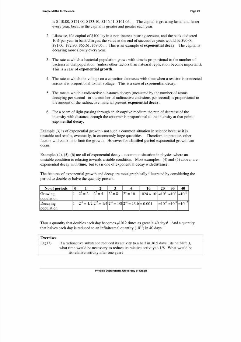
The features of exponential growth and decay are most graphically illustrated by considering theperiod to double or halve the quantity present:

No of periods 0 1 2 3 4 10 20 30 40

Growing

population

1 21 = 2 22 = 4 23 = 8 24 = 16 1024 ≈ 103 ≈106 ≈109 ≈1012

Decayingpopulation

1 2-1 = 1/2 2-2 = 1/4 2-3 = 1/8 2-4 = 1/16 ≈ 0.001 ≈10-6 ≈10-9 ≈10-12

Thus a quantity that doubles each day becomes ≈WLPHVDVJUHDWLQGD\V$QGDTXDQWLW\

that halves each day is reduced to an infinitesmal quantity (10-12) in 40 days.

Exercises

Ex(37) If a radioactive substance reduced its activity to a half in 36.5 days ( its half-life ),

what time would be necessary to reduce its relative activity to 1/8. What would beits relative activity after one year?





Graphs of exponential growth and decay, with fast and slow rates of change, are shown in the next

diagram.

0

1

2

3

4

5

6

7

8

9

10

0.0 0.5 1.0 1.5 2.0 2.5 3.0t

q

A useful graph of exponential decay is given in the following diagram. It is plotted using y = q

/ A , the ratio of the value of the quantity at time t to its initial value at t =0. Time is plotted as x =

α t ; thus the one graph is applicable for exponential decay of any rapidity. For t = 1/ α , the value

of y has decayed from its initial value of 1 to the value 1/e = 0.368, ( or, in terms of the quantity q ,

from its initial value A to the value A /e = 0.368 A ). The particular value of time, t = 1/ α, is called

the mean life , when the physical quantity has decayed to 1/e, ( ~ 1/3), of its initial value.

An alternative measure of the life-time of a decaying quantity in common use (especially for

radioactive decay) is the half-life, the time for the quantity to decay to 1/2 of its initial value.

Exponential Decay y = exp(-x)

0.0

0.1

0.2

0.3

0.4

0.5

0.6

0.7

0.8

0.9

1.0

0.0 0.5 1.0 1.5 2.0 2.5 3.0x

y

The graph shows the two different measures of life-time; their relationship is





693.0

life-meanx693.0life-half 2 / 1

=

== t

ExercisesEx(39) A radioactive substance has a half-life of 36.5 days. What is the value of the decay

constant α in (second)-1? If 1 mg was initially prepared how much would remain after

20 days, 100 days?

Ex (40) The decay constant for a resistance R discharging a capacitance C is given by α = 1/ RC .

How long does it take for a capacitance of 0.1 µF with a resistance of 0.1 MΩ across it

to discharge so that the voltage is reduced to 1/e of its initial value ? To 1/10 ?

13 THE LOGARITHM AND THE LOGARITHMIC FUNCTION

The logarithmic function is the inverse of the exponential function:

if y = 10 x then x = log y , ( sometimes written as log10 y)

or, using base e rather than base 10,

if y = e x then x = ln y , ( sometimes written as loge y ) .

We shall not have occasion to use the natural or Naperian logarithm to base e , but it may behandy to know that

ln y = 2.303 log y, so you can always convert from one to the other if need be.

You will however meet the logarithm to base 10 in two different ways.

13.1 LOGARITHMIC SCALE

There are occasions in science where we want to know how something behaves, not for equal

arithmetic steps of some quantity on which it depends, but for steps of equal multiples of thatquantity.

The scale -2 -1 0 +1 +2 +3 +4

is a LINEAR scale with arithmetic steps.

The scales

1/4 1/2 1 2 3 4 8

10-2

16

10-1 100 10+110+2 10+3 10+4 10+5

are LOGARITHMIC scales, with equal multiples for each step, the first using multiple steps

of 2 ( a binary scale ), and the second using multiple steps of 10 ( a decimal scale ).




Two cycles of a decimal logarithmic scale with subdivisions would look like

.1 .2 .4 .6 .8 1 2 4 6 8 10

13.2 The DECIBEL

One common example of a logarithmic function is the decibel scale used for measuring changes of

sound level. If a sound of physically measured intensity I 1 (measured in watts per square metre) is

increased to I 2, the sound level goes up by

decibel log101

2

=

I

I β

This method of describing a change of sound intensity, rather than simply by the ratio ( I 2 / I 1),

corresponds closely to how the nervous system and the brain interpret changes of loudness.

Exercises:Ex.(40) If a sound is changed in intensity from 0.01 Wm-2 to 0.03 Wm-2, what is the change

of the sound level in decibels?

Ex.(41) If the sound is changed from 0.03 Wm-2 to 0.01 Wm-2, what is the change of soundlevel?

You are now equipped with mathematical skills which will enable you to deal with much of

quantitative science. In the physical sciences you would need eventually to develop higher

level skills, and in many subjects you will also need skills in STATISTICS, which have not

been dealt with above.2002--01-10

simple maths for scientists

Documents