Simple and Efficient Geographic Routing aroundObstacles for Wireless Sensor Networks

Olivier Powell? and Sotiris Nikoletseas??

Computer Engineering and Informatics Department of Patras University andResearch Academic Computer Technology Institute (CTI), Greece.

Abstract. Geographic routing is becoming the protocol of choice formany sensor network applications. The current state of the art is un-satisfactory: some algorithms are very efficient, however they require apreliminary planarization of the communication graph. Planarization in-duces overhead and is thus not realistic for some scenarios such as thecase of highly dynamic network topologies. On the other hand, georout-ing algorithms which do not rely on planarization have fairly low successrates and fail to route messages around all but the simplest obstacles.To overcome these limitations, we propose the GRIC geographic routingalgorithm. It has absolutely no topology maintenance overhead, almost100% delivery rates (when no obstacles are added), bypasses large con-vex obstacles, finds short paths to the destination, resists link failureand is fairly simple to implement. The case of hard concave obstaclesis also studied; such obstacles are hard instances for which performancediminishes.

1 Introduction

Recent advances in micro-electromechanical systems (MEMS) have enabled thedevelopment of very small sensing devices called sensor nodes [1–3]. These aresmart devices with sensing, data-processing and wireless transmission capabil-ities meant to collaboratively form wireless sensor networks (sensor nets) in-strumenting the physical world by collecting, aggregating and propagating envi-ronmental information to regions of interest such as mobile users or fixed basestations possibly linked to a satellite or the Internet. Some applications imply de-ployment in remote or hostile environments (battle-field, tsunami, earth-quake,isolated wild-life island, space exploration program) to assist in tasks such as tar-get tracking, enemy intrusion detection, forest fire detection or environmental orbiological monitoring. Other applications imply deployment indoors or in urbanor controlled environments, for example with the purpose of industrial supervis-ing, indoor micro-climate monitoring (e.g. to reduce heating cost by detectingpoor thermal insulation of buildings), smart-home applications, patient-doctorhealth monitoring or blind and impaired assisting. Because of a few characteris-tics that differentiate them from otherwise similar ad hoc wireless nets such as? Work supported by the Swiss National Science Foundation, ref. PBGE2 - 112864.

?? Work partially supported by the E.U. IST program num. IST-2005-15964 (AEOLUS).

MANETS, sensor nets raise a multitude of algorithmic challenges [4, 5]. Amongcharacteristic that make sensor nets very different [6] are strong resource lim-itations (energy, memory, processing power), high-density and size (which canbe orders of magnitude greater than for other technologies) and the necessity tooperate unattended under the constraint of environmental hazard.Problem statement: We consider the problem of routing messages in a local-ized sensor net, a problem commonly called geographic routing (or georouting).We address the problem of finding a simple and efficient georouting algorithmwhich delivers messages with high success rate even in regions of low density(routing holes) and large communication blocking obstacles. The routing algo-rithms we allow ourselves to consider should be lightweight, on demand (thusmaking our algorithm all-to-all), efficient and realistic.On the importance of geographic routing: According to [7], “the most ap-propriate protocols [for sensor nets] are those that discover routes on demandusing local, lightweight, scalable techniques, while avoiding the overhead of stor-ing routing tables or other information that is expensive to update such as linkcosts or topology changes”. This is due to the severe resource limitations of sensordevices and the high dynamics of the ad hoc networks they spontaneously estab-lish. In view of this, geographic routing is very attractive [6, 7]. The early andsimple greedy georouting protocols [8] where messages are sent to the neighbourmaximising progress towards the destination meet those idealistic requirements:the only information required to route is, assuming the nodes are localized, thedestination of the message. One may wonder how realistic the assumption of lo-calized nodes is, and to what extent it confines georouting to a specialised niche.Our point of view is that “...geographic routing is becoming the protocol of choicefor many emerging applications in sensor networks...” [9] because location awarenodes are likely to be available since “...in many circumstances, it is useful andeven necessary for a node in a wireless sensor network to be aware of its locationin the physical world. For example, tracking or event-detection functions are notparticularly useful if the [sensor net] cannot provide any information where anevent has happened” [6]. Node localization is achievable through one of the manylocalization systems that use a combination of GPS like technology to localizea few beacon nodes followed by a distributed localization protocol [6, 7, 10–12].Interestingly, it turns out that georouting can even be used when nodes are notlocation aware by using virtual coordinates as was proposed in [13].State of the Art: The major problem of the early greedy georouting algorithms[8] is the so called routing hole problem [6, 7, 14] where messages get trapped in“local minimum” nodes which have no neighbours closer to the destination ofthe message than themselves. The incidence of routing holes increases as net-work density diminishes and the success rate of the greedy algorithm drops veryquickly with network density. In order to bypass routing holes (and obstacles),very ingenious georouting algorithms have been developed. The most successfulones are probably the celebrated GFG and GPSR algorithms [15, 16] (as well asincremental improvements such as GOAFR [17], c.f. [18] for details) which havethe very strong property of guaranteeing successful routing if the network is con-

nected. GFG and GPSR are very similar and were, to our knowledge, developedindependently. We use the encompassing term of face routing algorithms to referto GFG, GPSR and their incremental successors. They all share, as a centralidea, the use of a greedy propagation phase until the message reaches a localminimum. At this point a temporary rescue mode is used to escape the localminimum. The rescue mode uses (a variant of) the FACE algorithm originallydescribed in [15] where messages are routed along the faces of the polygons ofa planar subgraph of the communication graph. The use of a planar subgraph,which is necessary for face routing, is a crucial and restrictive characteristic: itimplies that a graph planarization component has to be included in the routingalgorithm. Until very recently, a major pitfall [19] of face routing algorithmswas that no practical planarization algorithm was known: “... all currently pro-posed geographic routing algorithms rely on idealized assumptions about radiosand their resulting connectivity graphs [...] which are grossly violated by real ra-dios [...] causing persistent failures in geographic routing, even on static topolo-gies” [20]. In a recent breakthrough paper [21] the first practical planarizationalgorithm with reasonable message overhead was proposed, lazy cross-link re-moval (LCR). Although reasonable, at least in static nets, LCR still induces ahigh topology maintenance overhead to discover impairing “cross-links”, c.f. [21].Another interesting approach is the BOUNDHOLE algorithm from [22] whichuses the TENT rule to discover local minimum nodes and then “bounds” thecontour of routing holes. Although it has a high overhead when compared tothe algorithm we propose, the information gained during the contour discoveryphase may be used for other application than routing such as path migration,information storage mechanisms and identification of regions of interest, c.f. [22]for details. Some other solutions are the probabilistic PFR, VTRP, LTP andCKN protocols [23–26]. These approaches are very different from face routingalgorithms in the sense that, at the the cost of accepting lower success rates (par-ticularly in low density networks), they induce very little topology maintenanceoverhead. Another drawback is that they fail to bypass large obstacles [27].Our approach: To overcome the limitations of previous approaches we proposea new algorithm: GeoRoutIng around obstaCles (GRIC), pronounced “Greek”in reference to its design location: the University of Patras in Greece. The mainidea of GRIC is to appropriately combine movement directly towards the destina-tion (to optimize performance) with an inertia effect. Inertia forces messages tokeep moving along the “current” direction and to closely follow the perimeter ofobstacles in order to efficiently bypass them. Inertia permits to get out of manyrouting holes and to bypass some quite strongly blocking convex obstacles. Tofurther improve our algorithm, a “right-hand rule” inspired component is used incombination with a virtual compass. The right-hand rule is a well known “wallfollower” technique to get out of a maze [28] which is also used for face rout-ing. However, unlike face routing algorithms, GRIC has the advantage of usingthe right-hand rule on the complete communication graph, thus eliminating theplanarization phase overhead. The right-hand rule permits to route messagesaround large obstacles, not only convex but also concave. It is useful even in the

absence of obstacles, making the success rate of GRIC close to 100% even for verylow density networks. We implement our algorithm and comparatively evaluateits performance against those of other representative algorithms (greedy, LTPand FACE). We focus on two performance measures: success rate and hop count.We study the impact on performance of several types of obstacles (both convexand concave) and representative regimes of network density.Strengths of our approach: GRIC is very simple (for example when comparedto face routing relying on LCR planarization) and thus easy to implement. Ithas a very high success rate, even in the case of low density networks. It is ca-pable of bypassing large emission blocking obstacles (although for the hardestobstacles performance decreases with network density) using a short path, closeto optimal in the absence of global knowledge of the network. It is particularlysuitable for highly dynamic networks where links go up and down, e.g. becauseof environmental fluctuation or network congestion. This follows from the factthat, for a start, GRIC has absolutely no topology maintenance overhead (theonly information required, at the node level, is a list of outbound neighbours)and from the fact that, as shown in our experiments, GRIC is not only robustwhen confronted with link failure: it also has the surprising property of actuallyperforming better when confronted to limited link instability. To our knowledge,the near 100% success rate of GRIC (without obstacles) and its effective obstacleavoidance property is unique among lightweight routing protocols. It also offersa competitive alternative to face routing, probably with a different dedicatedapplication niche: GRIC would be preferred for highly dynamic networks whereasface routing may be preferred in the case of more stable networks where the pla-narization overhead is paid off over time if the topology is static, implying thatplanarization does not need to be recomputed frequently. As a consequence, wefeel that GRIC considerably improves the state of the art of geographic routing.

2 The GRIC Algorithm

Sensor Net Model: When a node needs to route a message according to theGRIC algorithm, it needs some network topology information. More precisely,nodes should be aware of their 1-hop away outbound neighbours, as well as theircoordinates. In mathematical language, this is equivalent to assuming a directeddynamic communication graph (i.e. connectivity can change over time) embed-ded in the Euclidean plane. Although this may seem quite abstract at first sight,it is in fact very realistic: GRIC is a network layer protocol, it therefore relieson the data-link, MAC and physical layers. Many different MAC and data-linkprotocols exist, and although the study of the impact of different possible com-binations is beyond the scope of this paper, most of them would provide, atthe network layer, the level of abstraction we assume in this paper, c.f. [18] fordetails. A final minor assumption is that we allow messages to piggy-back O(1)bits of information encoding the position of the last node visited, the positionof the targeted message destination and a mark-up flag.Overview: Like face routing algorithms , GRIC uses two different routing modes:

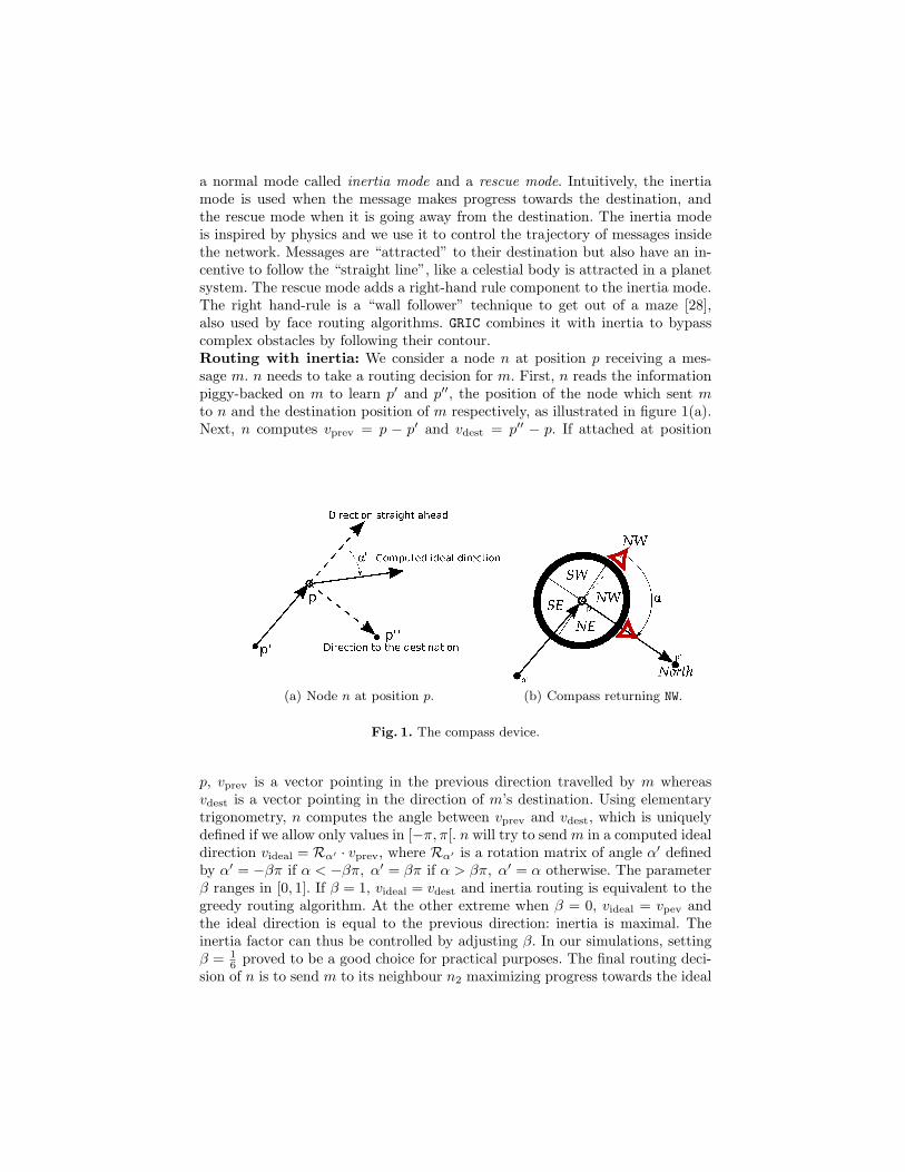
a normal mode called inertia mode and a rescue mode. Intuitively, the inertiamode is used when the message makes progress towards the destination, andthe rescue mode when it is going away from the destination. The inertia modeis inspired by physics and we use it to control the trajectory of messages insidethe network. Messages are “attracted” to their destination but also have an in-centive to follow the “straight line”, like a celestial body is attracted in a planetsystem. The rescue mode adds a right-hand rule component to the inertia mode.The right hand-rule is a “wall follower” technique to get out of a maze [28],also used by face routing algorithms. GRIC combines it with inertia to bypasscomplex obstacles by following their contour.Routing with inertia: We consider a node n at position p receiving a mes-sage m. n needs to take a routing decision for m. First, n reads the informationpiggy-backed on m to learn p′ and p′′, the position of the node which sent mto n and the destination position of m respectively, as illustrated in figure 1(a).Next, n computes vprev = p − p′ and vdest = p′′ − p. If attached at position

(a) Node n at position p. (b) Compass returning NW.

Fig. 1. The compass device.

p, vprev is a vector pointing in the previous direction travelled by m whereasvdest is a vector pointing in the direction of m’s destination. Using elementarytrigonometry, n computes the angle between vprev and vdest, which is uniquelydefined if we allow only values in [−π, π[. n will try to send m in a computed idealdirection videal = Rα′ · vprev, where Rα′ is a rotation matrix of angle α′ definedby α′ = −βπ if α < −βπ, α′ = βπ if α > βπ, α′ = α otherwise. The parameterβ ranges in [0, 1]. If β = 1, videal = vdest and inertia routing is equivalent to thegreedy routing algorithm. At the other extreme when β = 0, videal = vpev andthe ideal direction is equal to the previous direction: inertia is maximal. Theinertia factor can thus be controlled by adjusting β. In our simulations, settingβ = 1

6 proved to be a good choice for practical purposes. The final routing deci-sion of n is to send m to its neighbour n2 maximizing progress towards the ideal

direction videal, i.e. n2 maximizes the scalar product 〈videal|pos(n2)− p〉.Routing around obstacles: Our experiments show that inertia routing by-

−5 0 5 10 15 20 25

−5

05

1015

2025

Stripe

density = 7x position

y po

sitio

n

(a) GRIC, p = 0.95

−5 0 5 10 15 20 25

−5

05

1015

2025

U shape

density = 7x position

y po

sitio

n

(b) GRIC, p = 0.95

passes routing holes with high probability and routes messages around somelarge convex obstacles such as the one in figure 2(a). It is therefore used as thenormal routing mode of GRIC. However, more complex concave obstacles as infigures 2(b),2(c) and 2(d) cannot be bypassed by inertia routing and we there-fore add a rescue mode to GRIC. The first difficulty is to know when to switch torescue mode. A virtual compass device and the use of a flag fulfill this purpose.We keep notations of the previous section and consider that node n receives amessage m for which it needs to take a routing decision and describe below thesteps required to implement the obstacle avoidance feature of GRIC.• The compass device: n considers the north to be p′′, i.e. the destination of m,and it wants to know what cardinal direction describes the last hop of m: north-west, north-east, south-west or south-east, c.f. figure 1(b). The answer dependson α: the virtual compass indicates SW if α ∈ [−π,−π/2[, NW if α ∈ [−π/2, 0[, NEif α ∈ [0, π/2[ and SE otherwise.• The flag: Intuitively, when m is being routed around an obstacle the flag shouldbe up, otherwise it should be down. We metaphorically consider a walker fol-lowing the path along which m is routed. When the walker follows the pathand assuming m stays close to the obstacle’s contour, two cases can occur: theobstacle’s perimeter is either on the right or on the left of the walker. When thisis so, we say the message is routed around the obstacle according to the rightor left-hand rule respectively and GRIC acknowledges it by raising the flag andtagging it with SW or SE respectively. Formally, when n receives m, it starts byadjusting the flag’s value in the following way. If the flag is down, the algorithmlooks at the compass. If the compass points north, the flag stays down. However,if the compass points south, the flag is raised. and tagged with SW or SE respec-

−5 0 5 10 15 20 25

−5

05

1015

2025

Concave shape 1

density = 7x position

y po

sitio

n

(c) GRIC, p = 0.95

−5 0 5 10 15 20 25

−5

05

1015

2025

Concave shape 2

density = 7x position

y po

sitio

n

(d) GRIC, p = 0.95

Fig. 2. Typical behavior for different obstacle shapes.

tively. If the flag is up, n has two options: leave the flag up (without changingthe tag), or put the flag down. The flag goes down only if it was SW-tagged andthe compass points NW, or if the flag was SE-tagged while the compass points NE.• Mode selection: n receives the message m and it has to take a routing deci-sion. The decision is taken in steps. First, n adjusts the flag according to theprocedure described above. Next, it chooses whether to operate in the normalmode or whether it should switch to rescue mode. Only then will the routingdecision be made and we shall soon describe how, but we first describe how tochoose the routing mode. When the flag is down the normal mode is alwaysused. When the flag is up, it depends. Suppose the flag is up and for the sakeof simplicity let us assume it is SW-tagged, the other case being symmetric. Notethat by case assumption this implies that the compass does not point NW, sinceotherwise the flag would be down. Also, in this case, intuitively GRIC tries toroute around the obstacle using the right-hand rule. We next have to considertwo cases. If the compass points SW, recalling the definition of vprev, videal andα, it is easy to see that by case assumption videal is obtained by applying tovprev a rotation of angle α′ with α′ in [−π/6, 0], c.f. figure 1. In other words,inertia routing gives the message an incentive to turn to the right. This is consis-tent with the right-hand rule and GRIC thus chooses the normal routing mode.If the message points SE or NE, a similar reasoning shows that α′ is in [0, π/6]and that inertia routing will give an incentive for the message to turn left. How-ever, this will get the message away from the obstacle (in the expected casewhere the obstacle’s contour is indeed closely followed and kept on the right ofthe message). This is contrary to the right-hand rule idea and therefore GRICwill switch to rescue-mode.• The rescue mode: By case assumption, the flag is up and we assume withoutloss of generality the tag to be SW, i.e. the right-hand rule applies. The selec-

tion procedure previously described chooses rescue mode when inertia routingwould give the message an unwanted incentive to turn left by computing an α′

value in [0, π/6]. Intuitively, the rescue mode simply inverts the rotation angleα′ in the following way: let α2 = −sign(α)(2π − |α|). videal is then defined byvideal = Rα′

2·vprev, where α′

2 = βα2 and where β is the same inertia conservationparameter as the one used for inertia routing. Putting all things so far together,GRIC is formally described by the (non-randomized version of) algorithm 1.

Algorithm 1 GRIC, running on the node n which is at position pos(n).1: if the flag is down and compass indicates SW (or SE) then2: raise the flag and tag it with SW (or SE respectively)3: else if the flag is up and the tag is SW (or SE) then4: lower flag if the compass points NW (or NE respectively)5: Decide if mode should be normal or rescue {c.f. “Mode selection” subsection}6: if mode = normal then7: γ := α′ {c.f. “Routing with inertia” section}8: else if mode = rescue then9: γ := α′

2 {c.f. “Rescue mode” subsection}10: videal := Rγ · vprev

11: Let V be the set of neighbours of n and let V be an empty set.12: if running the random or non-random version of GRIC then13: set p = 0.95 or p = 1 respectively14: for all v ∈ V do15: add v to V ′ with probability p16: Send the message to the node n2 ∈ V ′ maximizing 〈videal|pos(n2) − pos(n)〉

Randomization and robustness: While designing GRIC, we decided to testits robustness when confronted tp link instability. We found that it performsbetter in the case of limited link instability. Although surprising and perhapscounterintuitive, this feature of GRIC is easy to understand. Indeed, routing fail-ure is likely to occur when a message deterministically starts looping around alocal minimum. A small random perturbation breaks GRIC’s determinism andmessages eventually escape the loop. This is a very nice property of GRIC whichalso suggests an easy way to improve its behavior in the context of stable net-works: each time n needs to take a routing decision for a message m it starts bytemporarily and randomly discarding each of its outbound links with probabilityp, c.f. line 12 of algorithm 1. For practical purposes experiments show the choiceof p = 0.95 to be good. Further decreasing the value of p, to the best of ourunderstanding, is tantamount to decreasing node density and thus performanceslowly decreases.

3 Experiments

We validate the performance of GRIC through extensive experiments. A singleexperiment consists of randomly deploying a sensor net. A message is then gen-

erated by a single node. The message has a destination, and the network tries toroute the message to it. The experiment is successful if the message reaches itsdestination before a given timeout value, it is deemed to have failed otherwise.To verify the quality of successful outcomes, we measure the length in hops of thepath that leads the message from source to destination. As a first experimentalvalidation of GRIC and for practical purposes we resolve ourselves to simulationrather than experimenting with real sensor nets: even small size sensor nets arestill quite prohibitively expensive and choosing and implementing a full protocolstack (MAC and data-link) on top of which our network layer algorithm operatesimplies a substantial amount of work which we delay for possible future work.Simulation platform: We developed a high-level simulation platform using theRuby programming language. As was previously explained, the GRIC algorithmis a network layer algorithm assuming a list of reliable collision free data-links tobe made available by lower protocol stack layers. This assumption is weak sincemost physical/MAC/data-link suites would indeed provide this level of abstrac-tion. We choose as a communication model the unit disc graph. Arguably, thismodel is the most commonly used for sensor net simulations. However, we ac-knowledge that this choice is not completely satisfactory and that more realisticcommunication graph models would be more appropriate. Defining a reasonablemodel suitable for simulation purposes is a challenging task. To our knowledge,only recently did the research community start to investigate this problem [29,30] and defining such a model is beyond the scope of this paper. Nevertheless, be-cause our algorithm is robust in the presence of link failure, because it requiresonly one-hop-away neighbourhood discovery, because it does not even requirelinks to be symmetric and because it implies absolutely no topology mainte-nance, we are confident that the unit disc communication graph is good enoughto give a reasonable approximation of the behavior GRIC will have in real sensornets.Simulation details: We deploy randomly and uniformly N sensor nodes inthe region of the Euclidean plane defined by

{(x, y) ∈ R2| − 5 ≤ x, y ≤ 25

}. The

density of the network d is defined as N/900. Using the unit disc graph model,the expected number of neighbours per node is thus close to d ·π. A message m isgenerated at the point (0, 10) and attached to the closest node. The destinationof m is (20, 0). m is propagated in the network according to the routing protocolconsidered. The experiment is considered successful if m gets within distance1 of its destination (there may not be a node at the exact destination of themessage). The outcome is a failure if m does not reach its destination in lessthan N steps. For precaution, we also consider the outcome to be failure if mapproaches within distance 1 from the border of the network.Preliminary results: We first consider the case where no obstacle is addedto the network. We considered the FACE algorithm of [15]. FACE is not themost competitive algorithm in the face routing family in terms of path length,because it always runs in rescue mode. However, like all face routing algorithmsit has the very strong “guaranteed delivery” property to always route a messageto its destination if a path exists from the source. In view of this, figure 3(a)

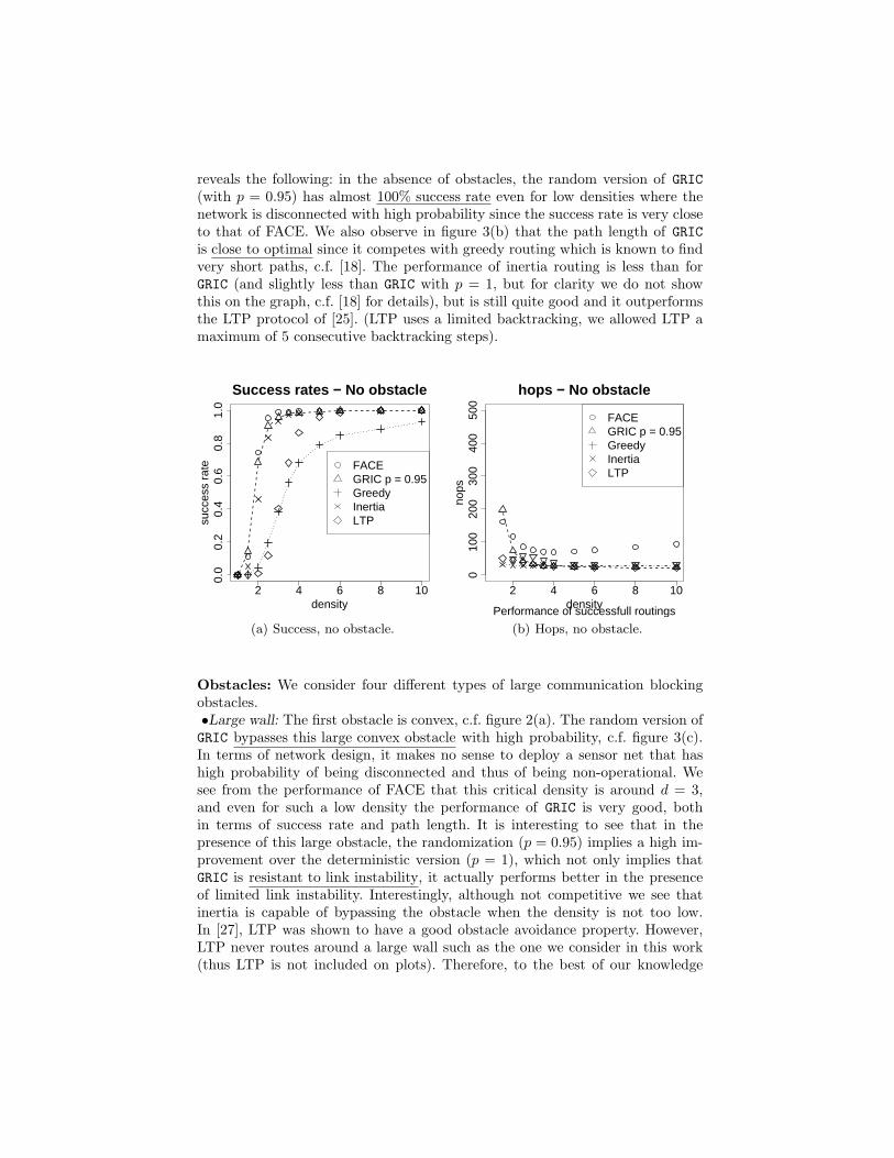
reveals the following: in the absence of obstacles, the random version of GRIC(with p = 0.95) has almost 100% success rate even for low densities where thenetwork is disconnected with high probability since the success rate is very closeto that of FACE. We also observe in figure 3(b) that the path length of GRICis close to optimal since it competes with greedy routing which is known to findvery short paths, c.f. [18]. The performance of inertia routing is less than forGRIC (and slightly less than GRIC with p = 1, but for clarity we do not showthis on the graph, c.f. [18] for details), but is still quite good and it outperformsthe LTP protocol of [25]. (LTP uses a limited backtracking, we allowed LTP amaximum of 5 consecutive backtracking steps).

2 4 6 8 10

0.0

0.2

0.4

0.6

0.8

1.0

Success rates − No obstacle

density

succ

ess

rate FACE

GRIC p = 0.95GreedyInertiaLTP

(a) Success, no obstacle.

2 4 6 8 10

010

020

030

040

050

0

hops − No obstacle

Performance of successfull routingsdensity

hops

FACEGRIC p = 0.95GreedyInertiaLTP

(b) Hops, no obstacle.

Obstacles: We consider four different types of large communication blockingobstacles.•Large wall: The first obstacle is convex, c.f. figure 2(a). The random version ofGRIC bypasses this large convex obstacle with high probability, c.f. figure 3(c).In terms of network design, it makes no sense to deploy a sensor net that hashigh probability of being disconnected and thus of being non-operational. Wesee from the performance of FACE that this critical density is around d = 3,and even for such a low density the performance of GRIC is very good, bothin terms of success rate and path length. It is interesting to see that in thepresence of this large obstacle, the randomization (p = 0.95) implies a high im-provement over the deterministic version (p = 1), which not only implies thatGRIC is resistant to link instability, it actually performs better in the presenceof limited link instability. Interestingly, although not competitive we see thatinertia is capable of bypassing the obstacle when the density is not too low.In [27], LTP was shown to have a good obstacle avoidance property. However,LTP never routes around a large wall such as the one we consider in this work(thus LTP is not included on plots). Therefore, to the best of our knowledge

2 4 6 8 10

0.0

0.2

0.4

0.6

0.8

1.0

Success rates − Large wall

density

succ

ess

rate FACE

GRIC p = 0.95GRIC p = 1Inertia

(c) Success, stripe.

2 4 6 8 10

010

020

030

040

050

0

hops − Large wall

Performance of successfull routingsdensity

hops

FACEGRIC p = 0.95GRIC p = 1Inertia

(d) Hops, stripe.

GRIC outperforms other lightweight georouting protocols, both in the presenceand absence of obstacles. In figure 3(d) we verify that path length is kept verylow, considering that the message has no a priori knowledge of the network anddiscovers the obstacle only when reaching it.•U shape obstacle: First of all, using a rule of thumb when looking in figures2(b) and in figure 3(f) shows that the deterministic version of GRIC (i.e. whenp = 1) rarely routes messages successfully to their destination but when it doesso it uses a near optimal path. In light of this observation, we conclude that GRIC(p = 0.95) bypasses this hard concave obstacle and uses a short path. However,the performance is only good when the network density is around 5 and higher.This is a medium density for sensor nets since, again, a density below 3 is prob-ably not acceptable in terms of network design since it yields a disconnectednetwork with non-negligible probability.• Concave shape 2: We skip results for the first concave shape in figure 2(c)because they are similar to those of the U shaped obstacle and turn to the finalobstacle. As seen in figure 2(d), this obstacle is problematic. The message isrouted out of the obstacle only to fall back in with high probability. As a con-sequence, the random version of GRIC only reaches acceptable performances forvery high network densities: success rate is bad for densities below 5 and pathlength is prohibitive even for densities below 8, c.f. figures 3(g) and 3(h).

4 Conclusion

We have studied geographic routing in the presence of hard communicationblocking obstacles and proposed a new way of routing messages which substan-tially improves the state of the art by somehow combining the best of two worlds:the lightweight (no topology maintenance overhead), robustness (to link failure)and simplicity of the greedy routing algorithm with the high success rates and

2 4 6 8 10

0.0

0.2

0.4

0.6

0.8

1.0

Success rates − U shape

density

succ

ess

rate

FACEGRIC p = 0.95GRIC p = 1

(e) Success, U shape.

2 4 6 8 10

010

020

030

040

050

0

hops − U shape

Performance of successfull routingsdensity

hops

FACEGRIC p = 0.95GRIC p = 1

(f) Hops, U shape.

obstacle avoidance features of face routing. The simplicity of GRIC suggests thatit would be a protocol of choice for routing in mobile networks. We shall in-vestigate this in future work. We have shown that GRIC resists (and actuallyperforms better) in the presence of limited link failure. Future work will investi-gate this matter more in depth, as well as the question of localization errors. Atfirst sight, there seems to be no reason to believe GRIC to be sensitive to them.GRIC proposes an alternative to the face family of protocols. We believe it hasa slightly different application niche and is preferable in the case of highly dy-namic networks (because frequent topology changes increase the topology main-tenance overhead of the planarization phase required for face routing), whereasface routing may be better in sparse but stable topologies where some overheadis acceptable. Deeper understanding of the differences between face and GRICrouting will require further investigation, more realistic communication graphmodels and possibly turning to real world experiments.

References

1. J. M. Rabaey, M. Josie Ammer, J. L. da Silva, D. Patel, and S. Roundy. Picoradiosupports ad hoc ultra-low power wireless networking. Computer, 2000.

2. B. Warneke, M. Last, B. Liebowitz, and K.S.J. Pister. Smart dust: communicatingwith a cubic-millimeter computer. Computer, 2001.

3. I. F. Akyildiz, W. Su, Y .Sankarasubramaniam, and E. Cayirci. Wireless sensornetworks: a survey. Computer Networks, 2002.

4. M. Haenggi. Challenges in wireless sensor networks. In Handbook of Sensor Net-works: Compact Wireless and Wired Systems. CRC Press, 2005.

5. D. Estrin, R. Govindan, J. Heidemann, and S. Kumar. Next century challenges:Scalable coordination in sensor networks. In Mobile Computing and Networking.ACM, 1999.

2 4 6 8 10

0.0

0.2

0.4

0.6

0.8

1.0

Success rates − Concave shape 2

density

succ

ess

rate

FACEGRIC p = 0.95GRIC p = 1

(g) Success, concave shape2.

2 4 6 8 10

010

020

030

040

050

0

hops − Concave shape 2

Performance of successfull routingsdensity

hops

FACEGRIC p = 0.95GRIC p = 1

(h) Hops, concave shape2.

Fig. 3. Summary of simulation results.

6. H. Karl and A. Willig. Protocols and Architectures for Wireless Sensor Networks.Wiley, 2005.

7. F. Zhao and L. Guibas. Wireless Sensor Networks, an Information ProcessingApproach. Elsevier, 2004.

8. G. G. Finn. Routing and addressing problems in large metropolitan-scale inter-networks. Technical report, Information Sciences Institute, 1987.

9. K. Seada, A. Helmy, and R. Govindan. On the effect of localization errors ongeographic face routing in sensor networks. In Information Processing in SensorNetworks, 2004.

10. J. Beutel. Location management in wireless sensor networks. In Handbook ofSensor Networks: Compact Wireless and Wired Systems. CRC Press, 2005.

11. J. Hightower and G. Borriello. Location systems for ubiquitous computing. Com-puter, 2001.

12. Pierre Leone, Luminita Moraru, Olivier Powell, and Jose Rolim. A localizationalgorithm for wireless ad-hoc sensor networks with traffic overhead minimizationby emission inhibition. In Algorithmic Aspects of Wireless Sensor Networks, 2006.

13. A. Rao, S. Ratnasamy, C. Papadimitriou, S. Shenker, and I. Stoica. Geographicrouting without location information. In Mobile Computing and Networking, 2003.

14. N. Ahmed, S. S. Kanhere, and S. Jha. The holes problem in wireless sensor net-works: a survey. SIGMOBILE Mob. Comput. Commun. Rev., 2005.

15. P. Bose, P. Morin, I. Stojmenovic, and J. Urrutia. Routing with guaranteed deliv-ery in ad hoc wireless networks. In Discrete Algorithms and Methods for MobileComputing and Communications, 1999.

16. B. Karp and H. T. Kung. GPSR: greedy perimeter stateless routing for wirelessnetworks. In Mobile Computing and Networking, 2000.

17. F. Kuhn, R. Wattenhofer, and A. Zollinger. Worst-case optimal and average-caseefficient geometric ad-hoc routing. In Mobile ad hoc Networking & Computing,2003.

18. Olivier Powell and Sotiris Nikoletseas. Geographic routing around obstacles in wire-less sensor networks. Technical report, Computing Research Repository (CoRR),2007.

19. Y.-J. Kim, R. Govindan, B. Karp, and S. Shenker. On the pitfalls of geographicface routing. In Foundations of mobile computing, 2005.

20. Y.-J. Kim, R. Govindan, B. Karp, and S. Shenker. Geographic routing madepractical. In Networked Systems Design & Implementation, 2005.

21. Y.-J. Kim, R. Govindan, B. Karp, and S. Shenker. Lazy cross-link removal forgeographic routing. In Embedded Networked Sensor Systems, 2006.

22. Q. Fang, J. Gao, and L. Guibas. Locating and bypassing holes in sensor networks.Mobile Networks and Applications, 2006.

23. I. Chatzigiannakis, T. Dimitriou, S. Nikoletseas, and P. Spirakis. A probabilisticforwarding protocol for efficient data propagation in sensor networks. Journal ofAd hoc Networks, 2006.

24. T. Antoniou, I. Chatzigiannakis, G. Mylonas, S. Nikoletseas, and A. Boukerche.A new energy efficient and fault-tolerant protocol for data propagation in smartdust networks using varying transmission range. In Annual Simulation Symposium(ANSS). ACM/IEEE, 2004.

25. I. Chatzigiannakis, S. Nikoletseas, and P. Spirakis. Smart dust protocols for localdetection and propagation. Journal of Mobile Networks (MONET), 2005.

26. I. Chatzigiannakis, A. Kinalis, and S. Nikoletseas. Efficient and robust data dissem-ination using limited extra network knowledge. In IEEE Conference on DistributedComputing in Sensor Systems (DCOSS), 2006.

27. I. Chatzigiannakis, G. Mylonas, and S. Nikoletseas. Modeling and evaluation ofthe effect of obstacles on the performance of wireless sensor networks. In AnnualSimulation Symposium (ANSS). ACM/IEEE, 2006.

28. A. Hemmerling. Labyrinth Problems: Labyrinth-Searching Abilities of Automata.B.G. Teubner, Leipzig, 1989.

29. Y. Yu, B. Hong, and V. Prasanna. On communication models for algorithm designfor networked sensor systems: A case study. Pervasive and Mobile Computing,2005.

30. A. Cerpa, J. Wong, L. Kuang, M. Potkonjak, and D. Estrin. Statistical modelof lossy links in wireless sensor networks. In Information processing in sensornetworks, 2005.