636-600 Neural Networks

• Instructor: Yoonsuck Choe

– Contact info: HRBB 322B, 845-5466, choe@tamu.edu

• Web page: http://faculty.cs.tamu.edu/choe

1

Textbook

• Simon Haykin. Neural networks and learning machines. Pearson

Education. Upper Saddle River, NJ, 2009.

• Older edition:

Simon Haykin, Neural Networks: A Comprehensive Foundation,

Second edition, Prentice-Hall, Upper Saddle River, NJ, 1999.

• Code from the book:

http://www.mathworks.com/books (click on

Neural/Fuzzy and find the book title).

• Text and figures, etc. will be quoted from the textbook without

repeated acknowledgment. Instructor’s perspective will be

indicated by “YC” where appropriate.

2

Other Textbooks and Books

• I. Goodfellow, Y. Bengio, and A. Courville, Deep Learning, MIT

Press, 2016.

• J. Hertz, A. Krogh, and R. Palmer, Introduction to the Theory of

Neural Computation, Addison-Wesley, 1991.

• C. M. Bishop, Neural Networks for Pattern Recognition, Oxford

University Press, 1995.

• M. A. Arbib, The Handbook of Brain Theory and Neural Networks,

2nd edition, MIT Press, 2003.

3

Course Info

• Grading: Exams: 60% (midterm: 30%, final: 30%); Assignments:

4% (4 written+programming assignments, 10% each); No curving:

≥ 90 = A,≥ 80 = B, etc.

• Academic integrity: individual work, unless otherwise indicated;

proper references should be given in case online/offline resources

are used.

• Students with disabilities: see the online syllabus.

• Lecture notes: check course web page for updates. Download,

print, and bring to the class.

• Computer accounts: talk to CS helpdesk.

• Programming: Matlab, or better yet, Octave

(http://www.octave.org). C/C++, Java, etc. (they should run on CS

Unix or windows) 4

Relation to Other Courses

Some overlaps:

• Machine learning: neural networks

• Pattern analysis: PCA, support-vector machines, radial basis

functions(?)

• (Relatively) unique to this course: in depth treatment of

single/multilayer networks, neurodynamics, committee machines,

information theoretic models, recurrent networks, etc.

5

Neural Networks in the Brain

• Human brain “computes” in an entirely different way from

conventional digital computers.

• The brain is highly complex, nonlinear, and parallel.

• Orgnization of neurons to perform tasks much faster than

computers. (Typical time taken in visual recognition tasks is

100–200 ms.)

• Key features of the biological brain: experience shapes the wiring

through plasticity, and hence learning becomes the central

issue in neural networks.

6

Neural Networks as an Adaptive Machine

A neural network is a massively parallel distributed processor made up

of simple processing units, which has a natural propensity for storing

experimental knowledge and making it available for use.

Neural networks resemble the brain:

• Knowledge is acquired from the environment through a learning

process.

• Inerneuron connection strengths, known as synaptic weights,

are used to store the acquired knowledge.

Procedure used for learning: learning algorithm. Weights, or even the

topology can be adjusted.

7

Benefits of Neural Networks

1. Nonlinearity: nonlinear components, distributed nonlinearity

2. Input-output mapping: supervised learning, nonparametric

statistical inference (model-free estimation, no prior assumptions),

3. Adaptivity: either retain or adapt. Can deal with nonstationary

environments. Must overcome stability-plasticity dillema.

4. Evidential response: decision plus confidence of the decision

can be provided.

5. Contextual information: Every neuron in the network potentially

influences every other neuron, so contextual information is dealt

with naturally.

8

Benefits of Neural Networks (cont’d)

6. Fault tolerance: performance degrades gracefully.

7. VLSI implementability: network of simple components.

8. Uniformity of analysis and design: common components

(neurons), sharability of theories and learning algorithms, and

seamless integration based on modularity.

9. Neurobiological analogy: Neural nets motivated by

neurobiology, and neurobiology also turning to neural networks for

insights and tools.

9

Human Brain

Stimulus → Receptors ⇔ Neural Net ⇔ Effectors → Response

Arbib (1987)

• Pioneer: Santiago Ramon y Cajal, a Spanish neuroanatomist who

introduced neurons as a fundamental unit of brain function.

• Neurons are slow: 10−3s per operation, compared to 10−9s of

modern CPUs.

• Huge number of neurons and connections: 1010 (recent estimate

is 1011) neurons, 6× 1013 connections in human brain.

• Highly energy efficient: 10−16J per operation in the brain vs.

10−6J in modern computers.

10

The Neuron and the Synapse

• Synapse: where two neurons meet.

• Presynaptic neuron: source

• Postsynaptic neuron: target

• Neurotransmitters: molecules that

cross the synapse (positive, negative,

or modulatory effect on postsynaptic

activation)

• Dendrite: branch that receives input

• Axon: branch that sends out output

(spike, or action potential traverses

the axon and triggers neurotransmit-

ter release at axon terminals).

11

Structural Organization of the Brain

Small to large-scale organizations

• Molecules, Synapses, Neural microcircuits

• Dendritic trees, Neurons

• Local circuits

• Interregional circuits: pathways, columns, to-

pographic maps

• Central nervous system

12

Cytoarchitectural Map of the Cerebral Cortex

Map-like organization:

• Brodmann’s cytoarchitectural map of the cerebral cortex.

• Area 17, 18, 19: visual cortices

• Area 41, 42: auditory cortices

• Area 1, 2, 3: somatosensory cortices (bodily sensation)

13

Topographic Maps in the Cortex

Visual Field Cortex

• Nearby location in the stimulus space are mapped to nearby

neurons in the cortex.

• Thus, it is like a map of the sensory space, thus the term

topographic organization.

• Many regions of the cortex are organized this way: visual (V1),

auditory (A1), and somatosensory (S1) cortices.

14

Models of Neurons

Neuron: information processing unit fundamental to neural network

operation.

• Synapses with associated weights: j to k denotedwkj .

• Summing junction: uk =∑m

j=1 wkjxj

• Activation function: yk = φ(uk + bk)

• Bias bk : vk = uk + bk , or vk =∑m

j=0 wkjxj (in the right

figure) 15

Activation Functions• Threshold unit:

φ(v) =

{1 if v ≥ 0

0 if v < 0

• Piece-wise linear:

φ(v) =

1 if v ≥ + 12

v if + 12 > v > − 1

2

0 if v ≤ − 12

• Sigmoid: logistic function (a: slope parameter)

φ(v) =1

1 + exp(−av)

It is differentiable: φ′(v) = aφ(v)(1− φ(v)).

16

Other Activation Functions

• Signum function:

φ(v) =

1 if v > 0

0 if v = 0

−1 if v < 0

• Sign function:

φ(v) =

1 if v ≥ 0

−1 if v < 0

• Hyperbolic tangent function:

φ(v) = tanh(v)

17

Stochastic Models

• Instead of deterministic activation, stochastic activation can be

done.

• x: state of neuron (+1 or -1); P (v): probability of firing.

x =

+1 with probability P (v)

−1 with probability 1− P (v)

• Typical choice of P (v):

P (v) =1

1 + exp(−v/T )

where T is a pseudotemperature. When T → 0, the neuron

becomes deterministic.

• In computer simulations, use the rejection method.

18

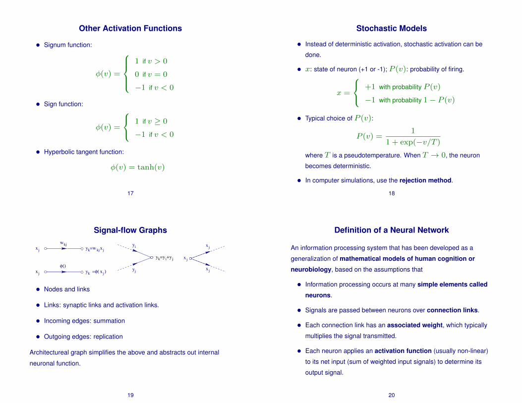
Signal-flow Graphs

yi

yj

yk=y i+y j

x j

kjwx j x j

x jyk

φ()=φ(

yk=w kj

)

x j

x j

x j

• Nodes and links

• Links: synaptic links and activation links.

• Incoming edges: summation

• Outgoing edges: replication

Architectureal graph simplifies the above and abstracts out internal

neuronal function.

19

Definition of a Neural Network

An information processing system that has been developed as a

generalization of mathematical models of human cognition or

neurobiology, based on the assumptions that

• Information processing occurs at many simple elements called

neurons.

• Signals are passed between neurons over connection links.

• Each connection link has an associated weight, which typically

multiplies the signal transmitted.

• Each neuron applies an activation function (usually non-linear)

to its net input (sum of weighted input signals) to determine its

output signal.

20

Signal-flow Graph Example: Exercise

• Turn the above into a signal-flow graph.

21

Feedback

Feedback gives dynamics (temporal aspect), and it is found in almost every part

of the nervous system in every animal.

yk(n) = A[x′j(n)](1)

x′j(n) = xj(n) + B[yk(n)](2)

Substitute (2) into (1) and we get

yk(n) =A

1− AB [xj(n)]

whereA/(1− AB) is called the closed-loop operator andAB the open

loop operator. Note thatBA 6= AB.

22

Feedback (cont’d)

Substitutingw forA and unit delay operator z−1 forB, we get

A

1 − AB=

w

1 − wz−1= w(1 − wz

−1)−1

.

Using binomial expansion (1− x)−r =∑∞

k=0

(r)kk! x

k & r = 1, we geta

A

1 − AB= w(1 − wz

−1)−1

= w

∞∑

l=0

wlz−l

.

From this, we get

yk(n) = w

∞∑

l=0

wlz−l

[xj(n)].

With z−l[xj(n)] = xj(n− l), yk(n) =∑∞

l=0 wl+1xj(n− l).

aPochhammer symbol (r)k = r(r+1)...(r+k− 1). Note: (r)k = k! when r = 1.

Feedback (cont’d)

yk(n) =∑∞

l=0 wl+1xj(n − l), so w determines

the behavior. With a fixed xj(0), the output yk(n) either

converges or diverges.

• |w| < 1: converge (infinite memory, fading)

• |w| = 1: linearly diverge

• |w| > 1: expontially diverge

24

Network Architectures

The connectivity of a neural network is intimately linked with the

learning algorithm.

• Single-layer feedforward networks: one input layer, one layer of

computing units (output layer), acyclic connections.

• Multilayer feedforward networks: one input layer, one (or more)

hidden layers, and ont output layer. With more hidden layers,

higher-order statistics can be processed.

• Recurrent networks: feedback loop exists.

Layers can be fully connected or partially connected.

25

Knowledge Representation

Knowledge refers to stored information or models used by a person or

a machine to interpret, predict, and appropriately respond to the

outside world.

• What information is actually made explicit.

• How the information is physically encoded for subsequent use.

Knowledge of the world consists of two kinds of information:

• The known world state: what is and what has been known –

prior informaiton.

• Observations (measurements) of the world, obtained by sensors

(they can be noisy). They provide examples. Examples can be

labeled or unlabeled.

26

Design of Neural Networks

• Select architecture, and gather input samples and train using a

learning algorithm (learning phase).

• Test with data not seen before (generalization phase).

• So, it is data-driven, unlike conventional programming.

27

Design of Representations

1. Similar inputs from similar classes should produce similar

representations, leading to classification into the same category.

2. Items to be categorized as separate classes should be given

widely different representations in the network.

3. If a particular feature is important, a larger number of neurons

should be involved in the representation of the item in the network.

4. Prior information and invariances should be built into the design of

a neural network with a specialized structure: biologically

plausible, fewer free parameters, faster information transfer, and

lower cost in building the network.

28

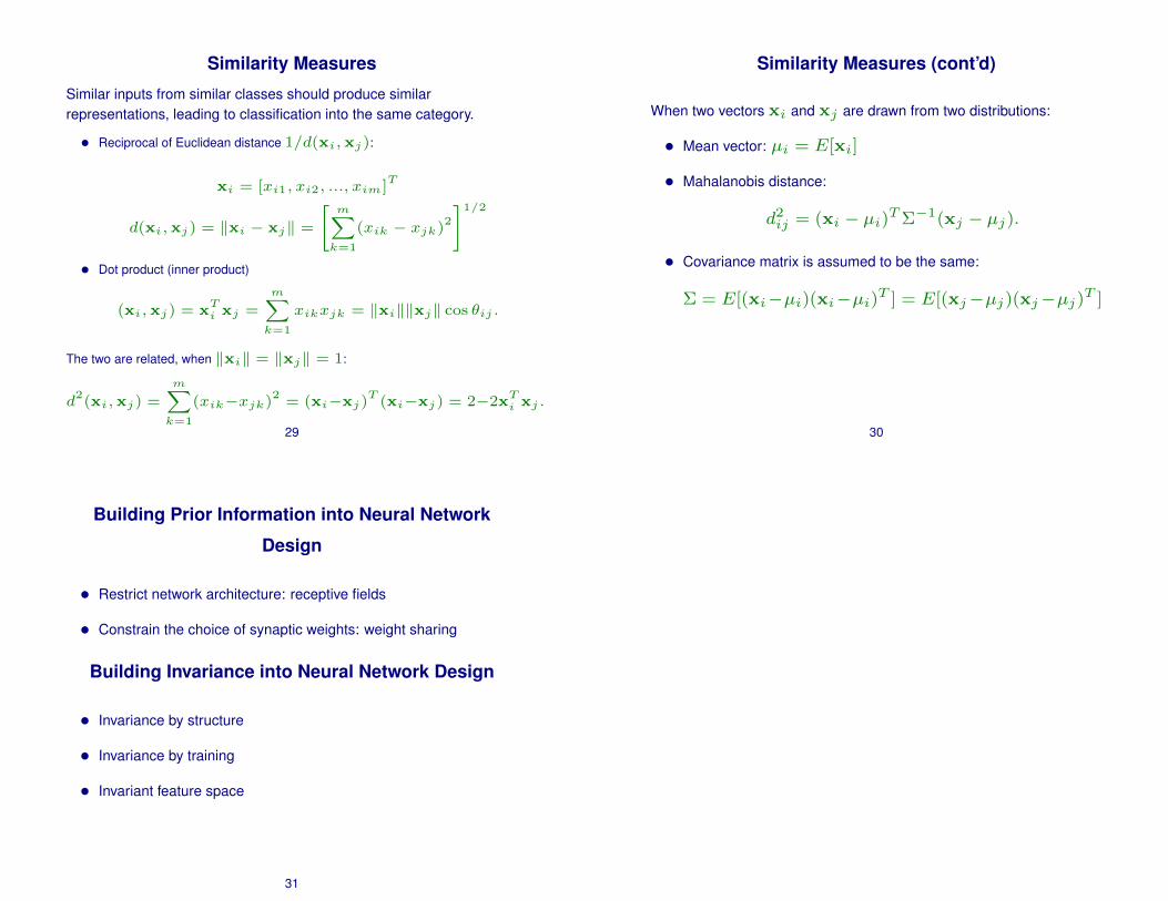
Similarity Measures

Similar inputs from similar classes should produce similarrepresentations, leading to classification into the same category.

• Reciprocal of Euclidean distance 1/d(xi,xj):

xi = [xi1, xi2, ..., xim]T

d(xi,xj) = ‖xi − xj‖ =

[m∑

k=1

(xik − xjk)2

]1/2

• Dot product (inner product)

(xi,xj) = xTi xj =

m∑

k=1

xikxjk = ‖xi‖‖xj‖ cos θij .

The two are related, when ‖xi‖ = ‖xj‖ = 1:

d2(xi,xj) =

m∑

k=1

(xik−xjk)2= (xi−xj)

T(xi−xj) = 2−2xT

i xj .

29

Similarity Measures (cont’d)

When two vectors xi and xj are drawn from two distributions:

• Mean vector: µi = E[xi]

• Mahalanobis distance:

d2ij = (xi − µi)T Σ−1(xj − µj).

• Covariance matrix is assumed to be the same:

Σ = E[(xi−µi)(xi−µi)T ] = E[(xj−µj)(xj−µj)T ]

30

Building Prior Information into Neural Network

Design

• Restrict network architecture: receptive fields

• Constrain the choice of synaptic weights: weight sharing

Building Invariance into Neural Network Design

• Invariance by structure

• Invariance by training

• Invariant feature space

31