1

Simin Hojat. PhD., MPhil

03/11/2014

Corporate Finance and Investment Theories

Abstract

In this paper, I reviewed theories of corporate finance and investment in business corporations.

The goal is to provide guidance for individual and institutional investors in their investment

decision making. I discussed various theories of corporate finance including capital budgeting

theories, capital structure theories, M&M theory of capital structure, and cost of capital theories,

as well as the concept of discounted cash flow (DCF), the net present value (NPV), the internal

rate of return (IRR) and the payback period techniques in regard with their appropriateness in

corporate investments decision makings. In regard with the investment theories, I reviewed

various theories of investment including Markowitz Portfolio Theory, Capital Asset Pricing

Model (CAPM), and Arbitrage Pricing Theory (APT).

Overview

In this paper, I reviewed theories of corporate finance and investment in business

corporations. The goal is to provide guidance for individual and institutional investors in their

investment decision making. Institutional and individual investors implement their investment

decisions through the capital market and in doing so they face three broad decisions: Asset

allocation decisions, choice of investments within an asset class, and risk management.

Corporations finance their investment activities in the capital market. Capital markets is a market

for meeting demand and supply of funds in which the length of time for investment is over a

year; this is in distinct from money market where the financial instruments with maturity of less

than a year are transacted. The role of capital market is very important in economic growth,

2

creating jobs, building infrastructure, and financing innovative ideas. Capital market is a market

for buying and selling equity and debt instruments to promote and grow individual businesses

and economic growth of a nation as a whole. Demand and supply in the capital market is

originated from Individual investors who purchase stocks or bonds and corporations that finance

their investment projects by issuing new securities. The design of the paper starts with the

definitions of important phenomena and then I explained and critically analyzed the important

theories of corporate finance and investment with a summary thought and conclusion on the

topic.

Definitions

Corporation: It is a distinct legal entity that has permanent life where the capital is

divided into shares of common or preferred stocks. In a corporation, shareholders have limited

liability and are not personally responsible for the debts or the claims against the corporation,

typically, the management of the firm is separated from the ownership. The invention of

corporate form of doing business, together with the emergence of the stock exchanges, has been

a major contributor to economic growth and development of the capitalist societies.

Expected rate of return: It is equal to benefits received in excess of the initial

investment as the percentage of the initial investment for a specific time. For example, for a

corporation, the expected rate of return at time t is the sum of price of the stock and the dividends

distributed at time (t+1) less the stock price at time t divided by the stock price at time

This can be shown as follows:

3

t

tttt P

PDPERE −+= ++ )()( 11 , where E is for expectation, R is rate of return, P is the price, D is

for dividend, and t represents the time.

Realized rate of return: It is the rate of return that is obtained from an investment on a specific

time; for example, the realized rate of return for a common stock at time t is

1

1

−

−−+=

t

tttt P

PDPR )( .

Capital expenditure: In contrast to operating expenditures, capital expenditure is the

outlays that firms incur to bring in benefits for periods longer than one year. In other words,

capital expenditures are outlays made for long-term investments.

Risk-free rate: It is a rate earned on the risk-free asset like interest rate on US

Government Treasury-Bills.

Risk premium: Risk premium of a stock is the excess return over the risk free rate for

the same holding time.

Financial leverage: It is a company’s level of debt that is the ratio of total long-term

debts of the company by its total assets.

Corporate Finance Theories

Corporations make long term investment in real assets, tangible and intangible, under the

heading of capital budgeting, capital structure, and the working capital management. The capital

budgeting decisions deal with the purchase of the firm’s tangible assets including long-term

machineries and buildings and intangible assets including trademarks, patents, and technical

expertise. The way that corporations decide on these long term investments is by comparing the

4

value of particular asset and its cost. The final decision depends on the economic efficiency of

the new machinery, it’s, timing, and risk of the future cash flows of investments.

On the other hand, the capital structure decisions are the methods of long-term funding

of investments. The corporation raises funds as the mix of long-term debt and equity to finance

its financial operations. Corporations evaluate the costs associated with each type of financing

and then, decide on the type and the amount of funding from equity or long term debt. However,

the working capital management is a day-to-day activity of corporations and its role is to ensure

that firms have adequate resources to continue operation without costly disruptions (Ross,

Westerfield, & Jordan 2001). For this purpose, corporations need short-term assets like cash

accounts receivable and inventories, as well as, short-term liabilities like accounts payable and

short-term borrowing.

Theories of corporate finance’s objective is to show how corporations can maximize their

share value of the company. To answer to this question, these theories have been looking for a

measuring metrics to guide them towards reaching this goals. Traditionally this metric that was

borrowed from economists has been profit maximization. However, the use of profit

maximization as an objective for financial management of the firms has been challenged on the

grounds that: (a) Profit is an accounting concept and may substantially differ from actual

economic value added for the corporation, (b) there is a difference between short term and long

term profit and it is not certain which one to be considered, (c) the stockholders who are in fact

own the equity in corporations are expecting to obtain financial gain and stock value appreciation

from the financial management of the firm. In other words, with respect to the separation of

management from the ownership in modern corporations, shareholders expect managers to act in

the best interest of the owners and to make financial decisions that increases the value of the

5

stock or equity. However, in cases that there is a conflict of interest between the long term goal

of the company and the interest of shareholders, it is dubious whether managers always act in

favor of stockholders. This conflict of interests between the owners as the principal and the

mangers as the agents is referred to as the agency problem leading to agency costs for the owners

of modern corporations (Brealy, Myers, and Marcus 2004).

Capital Budgeting Theory

Capital budgeting theories are referred to the theories that explain the capital expenditure

behavior of corporations. On the basis of economic theory and the assumption of firms’ rational

behavior, corporations invest in a new project only if net expected future benefits from the

investment are more than the initial cost of the investment. However, there is lack of

commensurate between benefits that occur from an investment over a period of time and

investment outlays in the initial year. In order to correct this, the present value of all future

proceeds is calculated by using a discount rate and then the result is compared with the initial

capital expenditure. Therefore, corporations need three data in order to evaluate an investment

project: The initial cost of the project, the expected net future benefits from the investment and

timing of such benefits, and the discount factor to be applied to future benefits for calculating

their present worth.

Discounted Cash Flow (DCF)

Corporations use the realized cash flows for measuring outlays and benefits in capital

budgeting theory, they do not use accounting expenses and profits. As a result one of the

methods that an investment project is evaluated is through the discounted cash flow, or the DCF,

methods. The cash flows that are relevant to a project are the incremental after-tax cash flows

6

expected to result from the capital expenditure and thus must be estimated by comparing the

after-tax expected cash flows to the firm with and without undertaking the project. There are four

components of cash flows: Initial investment, investment in net working capital, operating cash

flows, and the terminal cash flows. At the beginning of the project the relevant cash flow resulted

from the sum of the components is negative. However, as the project progress, net operating cash

flows become the main cash flow component and towards the end of the project life terminal

cash flow and recovery of net working capital constitute positive cash flows of the project

(Brealy, Myers, and Marcus 2004). These four components of relevant cash flow are derived

from the financial statements of the corporation: The initial investment, or initial capital

expenditure, is the sum of purchase price of new real assets plus the installation costs of the new

assets. The initial investment in DCF analysis is regarded as a cash outflow irrespective of

whether it is paid for by cash or financed through debt or issuance of new equity. Investment in

net working capital is defined as the difference between current assets and current liabilities of

the firm. Current assets are those assets that have high liquidity and can be converted into cash in

less than a year such as cash and cash equivalents, marketable securities, accounts receivable,

notes receivable, and inventory. Current liabilities are those obligations of the firm that must be

honored in less than one year and consist of accounts payable, notes payable, current portion of

the long-term debt, and some short-term accruals. Increase in net working capital, whether

required in the initial year of the new investment or in subsequent years, is regarded as relevant

cash outflow due to the project and treated as investment in networking capital. If in some years,

net working capital decreases due to implementation of the new project then the decrease would

be treated as relevant cash inflow.

7

Operating cash flow is net cash flows generated in every period during the life of the

project. Operating cash flow is calculated by adding back the depreciation expense and the

interest expense to the net after-tax profits. The reason for adding back the depreciation expense

is that it is a noncash expense representing part of the initial investment and the DCF method

already regards total initial investment as a cash outflow in the year that the project starts. The

reason for adding back interest expense is that interest expense is essentially a financing cash

flow, although in the accounting statement of cash flows it is regarded as operating cash flow.

The discounting of the cash flows at the firm’s or project’s cost of capital implicitly takes the

interest expense as well as the non-observable cost of equity capital out of the cash flow stream.

Doing so, makes evaluation of an investment project and the capital budgeting decision

independent of the financing of the project and capital structure decisions of the firm. Although

some authors, like Brealy, Myers, and Marcus (2004) or Gitman (2000), follow the accounting

method and do not add back the interest expense in calculating operating cash flows, Benninga

(2000) disagreed with them and asserted that, for the purpose of evaluating investment projects

through DCF method, not adding back the interest expense is methodologically incorrect and

leads to double counting of the interest expense. Terminal cash flow of the project is what the

project is worth at the end of its life. If the project is going to be salvaged and sold in the market

at the end of its life then the after-tax proceeds from its sale would be the terminal cash flow. If

the project is to be renewed, replaced, or its useful assets to be utilized for another project then

its potential market value would be treated as its terminal cash flow, which would be an

opportunity cost for the alternative investment projects.

8

The Net Present Value (NPV)

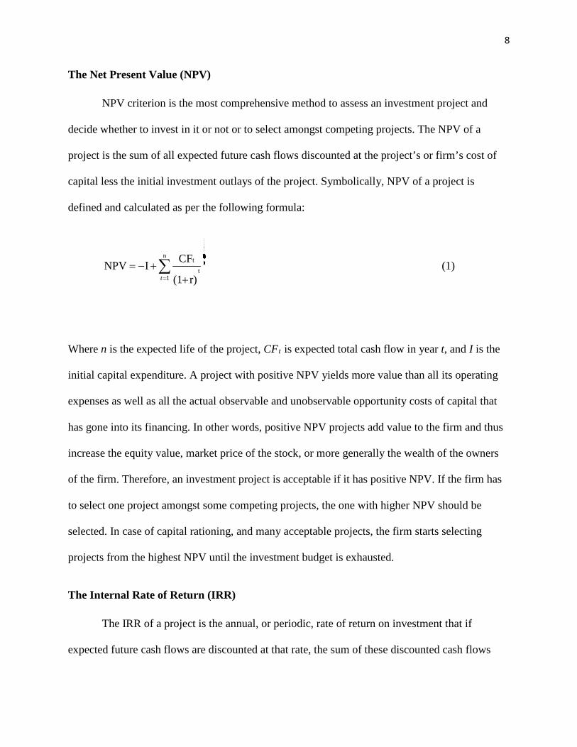
NPV criterion is the most comprehensive method to assess an investment project and

decide whether to invest in it or not or to select amongst competing projects. The NPV of a

project is the sum of all expected future cash flows discounted at the project’s or firm’s cost of

capital less the initial investment outlays of the project. Symbolically, NPV of a project is

defined and calculated as per the following formula:

n

tt

1

CFNPV I(1 r)t=

= − ++

∑ (1)

Where n is the expected life of the project, CFt is expected total cash flow in year t, and I is the

initial capital expenditure. A project with positive NPV yields more value than all its operating

expenses as well as all the actual observable and unobservable opportunity costs of capital that

has gone into its financing. In other words, positive NPV projects add value to the firm and thus

increase the equity value, market price of the stock, or more generally the wealth of the owners

of the firm. Therefore, an investment project is acceptable if it has positive NPV. If the firm has

to select one project amongst some competing projects, the one with higher NPV should be

selected. In case of capital rationing, and many acceptable projects, the firm starts selecting

projects from the highest NPV until the investment budget is exhausted.

The Internal Rate of Return (IRR)

The IRR of a project is the annual, or periodic, rate of return on investment that if

expected future cash flows are discounted at that rate, the sum of these discounted cash flows

9

will equal the initial investment outlays. In other words the IRR is the solution(s) to the

following equation:

n

tt

1

CF-I(1 )t

0IRR=

+ =+

∑ (2)

If IRR of a project is greater than the project’s or the firm’s cost of capital then the project is

acceptable and in the case of competing projects the ones with higher IRR will be preferred and

ranked higher for selection under capital rationing.

If the two techniques of investment decision making, the NPV and the IRR methods, lead

to consistent decision rules then the choice between the two would be a matter of convenience or

ease of communicating the subject. However, this is not always so. Using equation (1) if one

depicts NPV against the cost of capital r, then the point(s) at which the resulting graph intersects

the horizontal access is the IRR. If whenever the IRR is greater than the cost of capital the graph

of NPV stays above the horizontal axis then the NPV would be positive and both methods give

rise to consistent decisions with regard to one single project. This situation happens only if the

graph of NPV intersects the horizontal axis at only one point, that is, if the NPV function has one

solution only. The NPV function has only one solution if the time pattern of cash flows from the

project follows a conventional path. Conventional cash flow pattern occurs when there is only one

change of sign in the cash flows during the whole life of the project. Most projects yield

conventional cash flow pattern because usually the cash flows in the initial year(s) is negative and

then all other subsequent cash flows are positive. It is only in this case that the NPV function can

have one solution only and it is only in this case that the NPV and the IRR methods always lead

to the same decision for accept/reject decision of a single project. However, if the pattern of

expected future cash flows is not conventional it is possible to get multiple solutions for the IRR,

10

some of which could be inconsistent with the NPV criterion for specific values of the cost of

capital. The situation becomes even worse when it comes to comparing two projects and selecting

the more profitable one. Even when both projects have conventional cash flow patterns, the NPV

and the IRR methods lead to consistent results only when the graphs of the two NPVs are always

parallel. If the two functions intersect above the horizontal axis then the IRR method could lead to

selection of the project with smaller NPV for certain values of the cost of capital. So the general

conclusion is that the NPV method is the right method under all circumstances. The only

advantage of the IRR over NPV is that it could be easier to speak of projects’ profitability in

terms of rates of return than in terms of lump-sum dollar values. These ideas are illustrated

graphically in Figures 1-4 below.

11

NPV NPV

IRR IRR

Cost of Capital Cost of Capital

Case 1. Conventional cash flows: Case 2. Non-concentional cash flows: NPV and IRR are always consistent NPV and IRR are not always consistent

NPV NPV

IRRA IRRB

IRRB IRRA

Cost of Capital Cost of Capital

Case 3. Ranking of two projects: Case 4. Ranking of two projects: NPV and IRR are always consistent NPV and IRR are not always consistent

Figure 1. NPV and IRR consistencies

Payback Period Method

In the payback period method of investment decision making the firm estimates the

length of time that initial investment would be recovered and if that period is less than a target

payback period then the firm accepts the project. And for selection decisions the firm chooses the

project with the lowest payback period. The payback period method suffers from some serious

drawbacks that could lead to wrong decisions being made; and that is probably why large

corporations do not use this method for their large projects. By not discounting the future

expected cash flows, the payback period does not consider the time value of money and the risk

12

associated with the expected cash flows of the projects. It also ignores the cash flows after the

payback period. However, payback period method is simple and is employed for deciding on

small projects.

Capital Budgeting and Empirical Evidence

In their comprehensive survey of capital budgeting practices of US corporations Graham

and Harvey (2002) explored whether the theory and practice of corporate finance are consistent

or not? They survey 4,440 firms of different sizes from different industries and analyze results

received form 392 firms that responded to their survey. Despite previous surveys, they asked

whether firms used other techniques like payback period, accounting rate of return, and

profitability index method, and correlate the responses with specific features of the firms like,

size, leverage, and dividend policy. They found that the net present value and internal rate of

return were the most frequently used metrics in capital budgeting techniques; almost, 75% of

firms used net present value and internal rate of return. They also indicated that large firms used

NPV more than small firms. They also, stated that according to their research: Firms that pay

more dividends were using more of the NPV and IRR techniques; public companies were more

likely to use NPV and IRR than private corporations; small firms used the payback period more;

among small firms, CEOs without MBAs and mature CEOs used payback criterion more.

Capital Structure Theory

Capital structure theory is about the strategies that management adopts to have the

optimum combination of debt and equity that corporations employ to finance their assets; this is

typically shown as the ratio between debt-to total assets and also called the debt ratio or leverage

ratio. In deciding on the debt ratio, while keeping the total assets constant, corporations can pay

13

back some debts, incur more debts, or buy back part of their outstanding equities through the

capital market; this procedure is called capital restructuring. Capital restructuring decisions is an

independent activity by firms and typically, the best debt ratio for corporations is the one that

maximizes the wealth of its owners; that is, to maximizes the value of the shares of the company.

Therefore, there is a relationship between debt ratio and the equity value of the firm and the

corporation must find the one that maximizes the wealth of the firm; the optimal debt ratio can

be obtained in two different ways.

The first method refers to the firm’s total value which is equal to the firm’s total value

less the value of its debts; thus, the optimal debt ratio according to this definition is the one that

maximizes total value of the firm. This is measured through weighted average cost of capital

(WACC); that is, expected future benefits to be discounted with WACC which is the one that

constitutes both the cost of debt capital and the cost of equity capital. In other words, the less

WACC, the higher value of equity; thus, maximizing total value of the firm is essentially the

same thing as minimizing its weighted average cost of capital. In other words, according to this

method, the optimal capital structure can also be captured by finding the debt ratio which

minimizes the firm’s WACC. According to this model we have:

V= D+ E and A=V (3)

Where: D is the market value of debt; E is the market value of equity; V is the market value of

the firm; and A is the firm’s total assets.

The weighted average cost of capital of the firm (WACC) is the average of costs of

individual sources of finance weighed by their market values. Therefore:

14

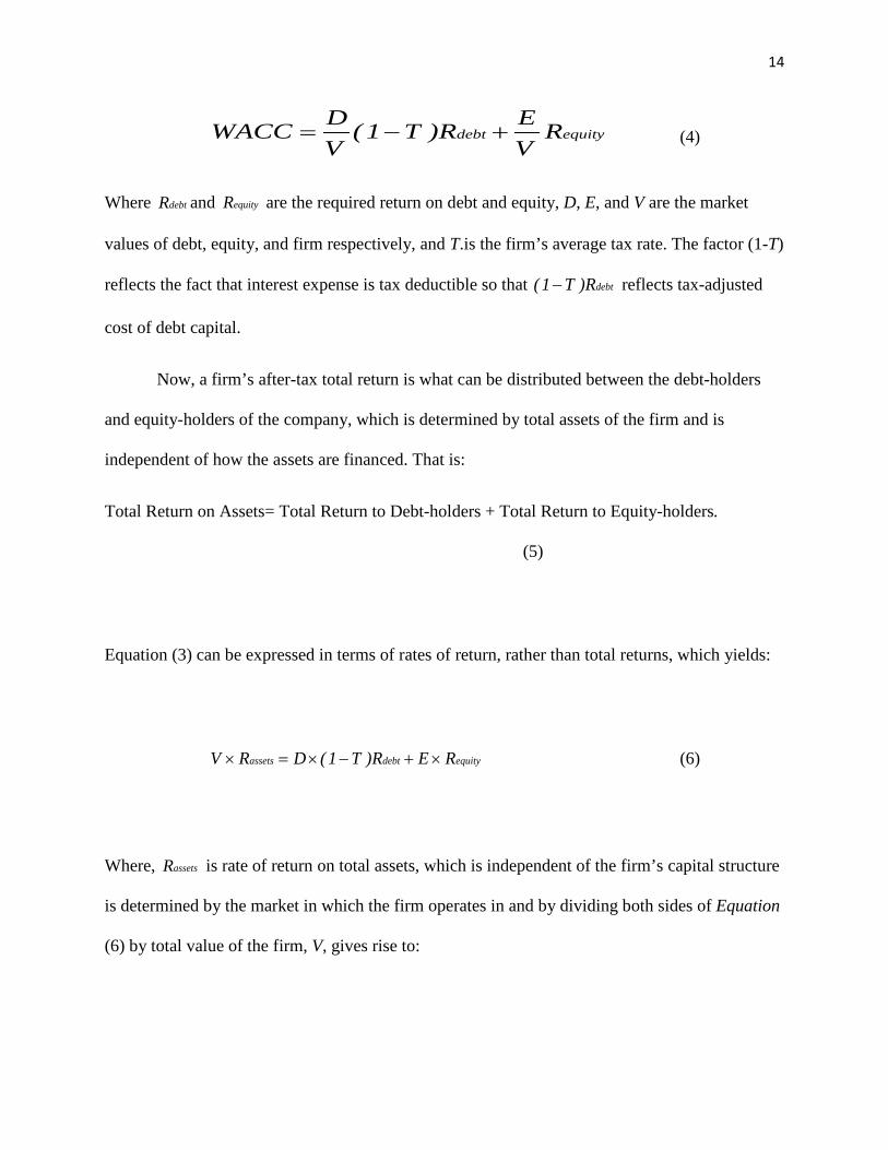
equitydebt RVER)T1(

VDWACC +−= (4)

Where debtR and equityR are the required return on debt and equity, D, E, and V are the market

values of debt, equity, and firm respectively, and T.is the firm’s average tax rate. The factor (1-T)

reflects the fact that interest expense is tax deductible so that debtR)T1( − reflects tax-adjusted

cost of debt capital.

Now, a firm’s after-tax total return is what can be distributed between the debt-holders

and equity-holders of the company, which is determined by total assets of the firm and is

independent of how the assets are financed. That is:

Total Return on Assets= Total Return to Debt-holders + Total Return to Equity-holders.

(5)

Equation (3) can be expressed in terms of rates of return, rather than total returns, which yields:

equitydebtassets RER)T1(DRV ×+−×=× (6)

Where, assetsR is rate of return on total assets, which is independent of the firm’s capital structure

is determined by the market in which the firm operates in and by dividing both sides of Equation

(6) by total value of the firm, V, gives rise to:

15

equitydebtassets RVER)T1(

VDR +−= (7)

It can be seen that the formula for WACC is the same in equation (7) and Equation (4). It

follows that for any specific total asset value; WACC is always the same as return on total assets

and is independent of capital structure. Therefore:

WACC= assetsR = Constant and determined by market conditions.

The other side of this independence of WACC from capital structure is value of the firm.

As the value of the firm is obtained by discounting expected future benefits to the debt-holders

and equity-holders of the firm at the WACC and because such expected benefits as well as the

WACC are both independent of the capital structure of the firm, it follows that the firm’s total

market value is independent of its capital structure. This prophesy was first fostered by two

Nobel Prize Winners, Franco Modigliani and Merton Miller in 1958, referred to as the M&M

propositions in finance and economic literature.

Modigliani and Miller

Modigliani and Miller (1958) put forward two proposals on capital structure policy; these

propositions were made on the assumption that there were no corporate taxes and capital market

was perfect. Later on in 1963, they expand their theory of corporate finance and allowed for the

effect of corporate taxes on the relationship between capital structure and value of the firm.

According to the first M&M proposition, if two firms have identical physical assets and identical

operations, assuming no corporate tax and perfect capital markets, the market values of the two

firms would be equal even with different capital structures. This is because, the two firms with

identical physical assets and identical operations means should have the same net operating

16

income and have the same market value. If one firm shows a higher market value than the other,

it becomes overvalued, and the other firm becomes undervalued; in this case, the security holders

of the overvalued firm will sell their holdings in the security market and buy the securities of the

undervalued firm. This trade off will make the market value of the two firms equal. M&M

proposition I is usually compared with different slicing of the same pie. If market value of the

firm is symbolized by a pie, then two firms with identical physical assets can be represented by

the same pie and capital structure representing the claims of various security holders of the firm

represents the way the pie is sliced and does not affect the size of the pie (Ross, Westerfield, &

Jordan, 2001).

In the second M&M proposition that derived from the first one, Modigliani and Miller

explained the effect of capital structure on the rate of return and market value of equity capital.

Assuming no taxes, Equation (7) mentioned in the previous section will become:

equitydebtassets RVER

VDR += (8)

Rearranging the terms in Equation (8) to solve for return on equity, equityR , and considering that

V=D+E, the following relationship is obtained:

EDRRRR )debtasset(assetequity −+= (9)

According to Equation (7) the cost of equity is determined by: The required rate of return on the

firm’s assets; the firm’s excess return on assets over the cost of debt; and the firm’s debt-equity

ratio. In this case, if return on assets is more than the cost of debt, use of more leverage in the

capital structure will raise the rate of return on equity. On the contrary, if return on assets is less

that the cost of debt, higher leverage will reduce return on equity; indeed, use of leverage

17

increases both the risk and the return of the equity-holders of the company. Equation (7) also

implies that the risk of the equity depends on both: Business risk, the risk of the firm’s operations

or Rasstet and financial risk, the risk associated with capital structure or D/E.

Dividend Policy and market valuation

The earning of the firm is either distributed in the form of dividends to the shareholders

or is kept in the firm as retained earnings which are used as means of financing the costs of the

corporation. Since, the higher the dividend pay-out, the lower is the retained earnings and the

higher is the need for other sources of financing by the firm, the dividend policy has implications

on the financing decision of the firm and the theories that describe this area of finance are called

the dividend policy theories. The focus of these theories is on maximizing the wealth of the

shareholders and the impact of dividend policy on the market valuation of the firm, specifically

on the firm’s stock price. As a whole, these theories are categorized into two major groups: 1-

irrelevance dividend proposition that suggests no relationship between dividend policy and the

firm’s market value; 2- those that regard dividend policy being relevant and affecting the firm’s

value; 3- the residual theory of dividends.

The Dividend Theories

The idea of dividend irrelevance theory was first introduced by Modigliani and Miller

(1961). They stated that on the assumption that capital markets are perfect, there are no

transaction costs, and no taxes, the dividend policy of the firm neither affects the market value of

the firm nor the wealth of its stockholders; this is because, the value of the firm is determined by

the earning power of the firm’s assets and its cost of capital and because stockholders of the firm

can always create home-made dividend. According to the Modigliani and Miller analysis of the

18

irrelevance theory, if two identical firms with identical future expected cash flows, one paying

out dividend and the other one retaining all earnings, the dividend paying firm must issue new

shares to finance its investments if its debt level is to be unchanged. Therefore, if the dollar

amount to be raised from the new issue is equal to the dollar amount of dividends paid out, the

market value of the firm will remain unchanged. On the other hand, with issuing new shares the

market price per share declines because, there are more shares while total earnings is the same;

since the amount of dollar decline in price per share is equal to the dollar dividend paid, total

wealth of an individual shareholder will not be affected by the dividend policy. Moreover, in

case that the dividend paying firm does not issue new shares to continue its investment, its share

price falls due to shortage of investment; again the total wealth of the individual share- holder

would be unchanged. Therefore, it makes no difference to the individual shareholder whether to

have a higher stock price and no dividend or dividend and lower stock price; in other words,

dividend policy does not matter and is irrelevant (Modigliani and Miller, 1961).

The theory of Modigliani and Miller has been challenged by the oppositions on two

grounds: The first challenge comes from the fact that share prices will rise after dividend pay-out

because of the informational content of dividends with respect to future earnings and the fact that

a dividend pay- out signals to the share-holders as the expected future growth of the company by

managers. The second argument, which is called the clientele effect proposition, is based on the

fact that investors have different expectations for dividends and capital gain and purchase those

stocks that meet their expectations. Once all investors are happy with the dividends they receive,

no firm can cause its stock price to rise by increasing its dividend pay-out (Gitman, 2000).

The proponents of this view argue that dividend policy does matter and it affects the

value of the firm and the wealth of its shareholders. One argument which is in favor of high

19

dividends pay-out and, known as birds-in-the-hands argument, proposes that investors are

generally risk-averse and prefer current dividends pay-out to uncertain future dividends or capital

gains; consequently, investors assign lower discount rate to the high dividends pay-out than the

low dividends pay-out. Thus, ceteris paribus, a firm that pays high dividends will have higher

share prices and market value than a firm with low pay-out. However, there is a difference

between tax treatments of dividend income and capital gain, dividends are taxed as they are paid

while capital gain tax is deferred until the stock is sold in the future and the tax rate on dividend

income in the US is higher than the tax rate on capital gain. Thus, all other things being equal, it

is concluded that the shareholders expected future after-tax benefits to be higher for the low-

dividend-paying firm than the high-dividend-paying firm; therefore, the firm that is paying lower

dividends might show higher share price (Gitman, 2000).

There is also this school of thought that considers dividends as a residual payment; the

reason for this argument is that they presume that firms only pay dividends when other financial

need of the company is met. Therefore on this analysis when firms have more business

opportunities, they should pay less dividend and one can postulate that if a firm has no

investment opportunity during a time period, the dividend pay-out should be 100%. Thus,

dividend policies should not influence the expected rate of return and value of the firm; a

conclusion that suggests dividends policy is irrelevant (Gitman, 2000).

Part Two: Theories of Investment

Theories of investment are concerned about the ways investor make their investment

decisions and implement it through the capital market; in this regard, they are facing with three

distinct and interconnected decisions. These decisions are: 1-Asset allocation decisions, which is

allocation of funds for investment within broad choice of assets including equities, cash, bonds,

20

and so on. 2- Investment choices within an asset such as deciding on what stock to buy within

the class of equity. 3- risk management that persuade investors to diversify their portfolio

between different assets, within each class of assets, and use of derivative instruments like stock

or bond options and futures to hedge against possibility of loss. Investments theories are

classified as: The ones that describes the investors’ behavior individually and as a group, positive

approach and the ones that describe how a rational investor should behave in order to achieve

their objectives given various constraints including their specific risk tolerances, normative

analysis.

The theories of investment in relation with asset allocation were based on the pioneering

work of the Noble Prize Winner Harry Markowitz (1952) on his portfolio selection theory.

Investments theories in relation with selecting a specific asset within a class, either in an

individual asset or a portfolio of assets in the class, were basically explained by the theories of

asset pricing or asset valuations. The major theories that describe the way that assets are priced

in the capital market are capital asset pricing model (CAPM), arbitrage pricing theory (APT),

and the recently devised real options theory which has not yet gained much popularity. In regard

with the risk management, both Markowitz portfolio selection theory and CAPM might be used

as guide for the diversification aspect of risk management. Moreover, there is the Black-Scholes

options pricing theory that explains how stocks or bond options are priced in the capital market

and how they can be used by investors to hedge their investments against possible losses or

reduce the risk of loss.

21

The Portfolio Theory

Harry Markowitz

Markowitz (1952) who is often called the father of modern portfolio theory was the

pioneer in the modern portfolio theory (MPT) and won the 1990 Noble Prize in economics for it.

His portfolio selection theory was about the design and construction of a diversified portfolio of

different assets by investors. According to Markowitz an investor selects her/his portfolio on the

basis of the future expectation on the performance of assets which s/he will obtain as a result of

historical performances of assets as well as the investor’s experiences with available securities.

Then, on the assumption that expectations are already decided by investors, Markowitz’s model

describes how investors select a portfolio that minimizes their risk. He used the variance of

returns or standard deviation of returns in his model and it is now used as a measurement of

investment risk by most theoreticians and investors in the field of investment management.

Markowitz (1952) assumed that the rates of return of individual assets vary together and

therefore, it is mathematically possible to build a matrix of variance-covariance for all risky

assets and thereby calculate the risk involved in each portfolio. Markowitz asserted that for each

individual with a given risk aversion, there is an optimum combination of risky assets that entails

the minimum risk. In other words, every individual investor can have a desirable portfolio of

assets that yields the maximum rate of return. He named these portfolios that are constructed on

the basis of optimal weights efficient portfolios, this is the base for his famous definition of the

efficient frontier. Markowitz, based on the assumption that investors are risk-averse, concluded

that each investor will choose a portfolio on the efficient frontier that fits her/his risk-returns

profile.

22

The efforts by investors in constructing their optimum portfolios lead to the buy and sell

decisions of securities in the in the capital market and set the prices in the stock market.

Moreover, Markowitz talks about expected return-variance, or E-V, rule and argued that this rule

better explains investments decision-making than the expected return maximization rule,

because, the E-V hypothesis implies both diversification and the right diversification for the right

reasons. In a nutshell, the Markowitz’s model provided the guideline for investors to create an

optimal portfolio of assets which is based on: Their risk tolerance, the expected returns on

securities, the variances (or standard deviations) of securities’ returns, and the covariance or

correlations between security returns. Although, Markowitz model was a sound theory of

investment, its empirical testing was very difficult, but it inspired other researchers to follow the

Markowitz’s risk-return idea and transfer it into less complicated models.

In a mathematical formula, if there are n risky securities from which investors could

select and construct their portfolios, where, one-period holding rate of return from investing in

security i is Ri and each Ri is a random variable with known probability distribution. Then, the

information on the probability distribution functions of each Ri allows the researcher to calculate

the expected value of returns, the expected value of variances of returns for every security, and

the expected values of covariance of returns or correlations between any two securities.

Moreover, on the basis of assumption that the future probabilities of returns are the same as the

past, the researcher can estimate the historical data of one-period rates of returns and obtain the

expected values of returns and their expected variances and covariance. Therefore, in Markowitz

model the following information is available to all investors at any point in time about the all

securities available in the market:

23

Thus, according to this model, an investor can construct her/ his portfolio for the specific

amount of funds and decides what proportion of her/his amount of invest

µI =E (Ri ) Expected of return of security i = average of historical returns of security i,

σI 2 =Expected variance of returns of security i = variance of historical returns of security i

ρi j =Expected correlation coefficient between returns on stock i and returns on security j =

historical correlation coefficient between returns on security i and returns on security j.

(9)

Thus, according to this model, an investor can construct her/ his portfolio for the specific amount

of funds and decides what proportion of her/his amount of investment to invest in each security.

Then, if we denote, the percentage of fund to be invested in security i by wi, we have the

following set of equations:

Expected return of the portfolio=

∑=

=++=n

iiinnp wwww

12211 ........ µµµµµ (10)

Expected variance of return of the portfolio=

)......(2)......( 111211221222

121

2nnnjiijjinnp wwwwwwww σσρσσρσσρσσσ +++++=

Or:

∑∑∑= +==

+=n

i

n

ijjiijji

n

iiip www

1 11

222 2 σσρσσ (11)

And

24

1...............21 =++ nwww (12)

Where the weights in Equation 12 were all non-negative and less than or equal to one and short-

sale is not permitted; if short-sale is allowed, some weights were negative and some were not,

but the sum total of all weights still adds up to one.

When there were many assets in the portfolio it was preferred by the model to use a

matrix form which makes it easier to calculate portfolio’s expected return and n matrix form as

and the equations 10-12 can be written as:

RW Tp =µ (13)

WW Tp σρσσ =2 (14)

1=IW T (15)

Where, WT is the transpose of W and I is the unit column vector with n rows.

To do so, first one of the weights w can be expressed in terms of other w’s and substituted into

equations 10 and 11. Then from equation 10 another of the w’s can be expressed in terms of p

and then substituted into equation 11. The result would be a quadratic relationship between

portfolio’s risk and return of the general form:

22ppp cba µµσ ++= (16)

Where, a, b, and c contain (n-2) of the w’s. With p on the x-axis and p on the y axis, plot of

equation 14 would be a series of hyperbolas, each of which represents a specific combination of

the values of the portfolio weights, w’s. The set of all such possible portfolios was called the

feasible set by Markowitz. Simply putting it, the feasible set consists of all portfolios for which

25

the sum of the w’s adds up to 100%. In the literature on Modern Portfolio Theory, the mean-

variance efficient portfolios, is referred to as the efficient frontier and it is referred to as the part

that would gain a higher expected return for the investor (Bodie, Kane, & Marcus, 1993).

Therefore, according to Markowitz (1952) rational investors do and should select a portfolio

from the efficient frontier. All that the investor needs to do is to decide how much risk he or she

is willing to take and then the efficient frontier provides him or her with the optimal portfolio for

that level of risk.

In addition to the notion of mean-variance efficient portfolios, Markowitz’s theorem had

two other important theoretical implications for the practice of portfolio management. One

implication, easily derived from the formula for portfolio variance (Equation 10) is that the lower

the correlations between stocks in a portfolio the lower would be total risk of the portfolio. This

is evident from the second term in the right hand side of Equation 10 which shows that even if

the variances of individual securities are kept the same, lower correlations lead to lower total

portfolio’s variance. This conclusion is very important for the practice of portfolio management.

It implies that from the portfolio’s perspective, the risk of an individual asset should not be

assessed by its own variance but rather by how much it adds to the portfolio’s total risk when it

is added to a portfolio. Therefore, adding a high risk-high return security to a portfolio will

increase portfolios’ expected return, according to Equation 10, while if it has low correlations

with other securities in the portfolio it will relatively add less risk to the portfolio or even could

reduce total risk if it has negative correlations with some of the securities. The second

implication also derived from Equation 10 but not as evident as the first one, is that the more the

number of securities in the portfolio the lower would be the total risk of the portfolio. This

conclusion is usually proved mathematically by considering the special case where all the

26

weights in the portfolio are equal, that is, when all the wi’s are equal to 1/n. In this case the

portfolios’ variance p2 from Equation 11 can be reduced to:

j

n

i

n

ijiiji

n

ip nn

σσρσσ ∑ ∑∑= +==

+=1 1

22

12

2 121 which, given that there are n variances and

N (n-1)/2 correlations, this can be simplified to:

Covn

nnp

11 22 −+= σσ (17)

Where, 2σ is the arithmetic average of variances of returns of individual securities and Cov is

the arithmetic average covariance of returns between every two securities in the portfolio.

The first term in Equation 17 above represents average risk specific to individual

securities and as the number of securities in the portfolio, n, increases the specific risk decreases

and ultimately becomes zero. Thus, adequate diversification eliminates specific risk of securities,

or as usually described in the literature, specific risk can be diversified away. The second term in

Equation 17, however, cannot be diversified way. When n becomes very large the coefficient of

the second term approaches 1 and therefore total portfolio risk approaches the average

covariance of the securities in the portfolio. Securities’ returns covary when there are some

general factors that affect the returns of all securities and that is why the second term in Equation

15 is referred to as the systematic risk of the portfolio. Systematic risk is non-diversifiable and its

size depends on the degree of correlations between securities’ returns. If on average the

correlations between securities’ returns turn out to be zero then the second term in Equation 10,

that is the systematic risk, will also be zero with adequate diversification. In this case one might

create a fully hedged portfolio through diversification. On the other hand, if on average the

27

securities in the portfolio show perfect positive correlation then average covariance becomes the

same as average variance, that is Cov =σ 2 , and the systematic risk equates average variance of

the securities’ return. In this case diversification has no risk reduction benefit no matter how

many securities are added to the portfolio. (Bodie, Kane, & Marcus, 1993).

James Tobin

Another contributor to modern portfolio theory was James Tobin (1958) who

introduced the role of cash or a risk-free financial asset into the process of optimal

portfolio selection and eventually in determination of equilibrium prices in the capital

market. Tobin considered the case where the investor allocates his or her wealth between

a risk free asset and one of the portfolios on the efficient frontier. Subsequently Sharpe

(1964) generalized Tobin’s idea of the risk free asset by assuming that all investors can

both lend (invest) or borrow at the same risk free rate. This idea of investing in a portfolio

on the efficient frontier together with the possibility of lending and borrowing at the risk

free rate led to a striking contribution to Markowitz’s portfolio theory and formed the

basis for the development of capital asset pricing model (CAPM).

Capital Asset Pricing Model

The theories on asset pricing and asset price determination in the stocks and bonds

markets are the most important area of investment theories. The problem with asset evaluation in

the capital market stems from the fact that the expected return on capital entails time; that is, the

future flow of income is the decider in present asset pricing. Economic theory suggests that the

value of asset is determined by three factors: The future cash flows obtained from asset, the

length of time that cash flows are expected, and a discounted rate to be used to calculate the

28

present value of all the future cash flows (Cochrane, 2001). Since, different assets have different

degree of uncertainty and require different expected rates of return, they entail different degrees

of risks. Thus, two assets with the same cash flows might have different prices in the capital

market if investors decide that one is riskier than the other. The relationship between expected

rate of return of an asset and the risk involved in the asset is one of the fundamental issues of

asset pricing both theoretically and practically. The Capital Asset Pricing Model (CAPM) which

is the most controversial and most referenced theory in theories of investment has thoroughly

analyzed the relationship between risk and expected rate of return.

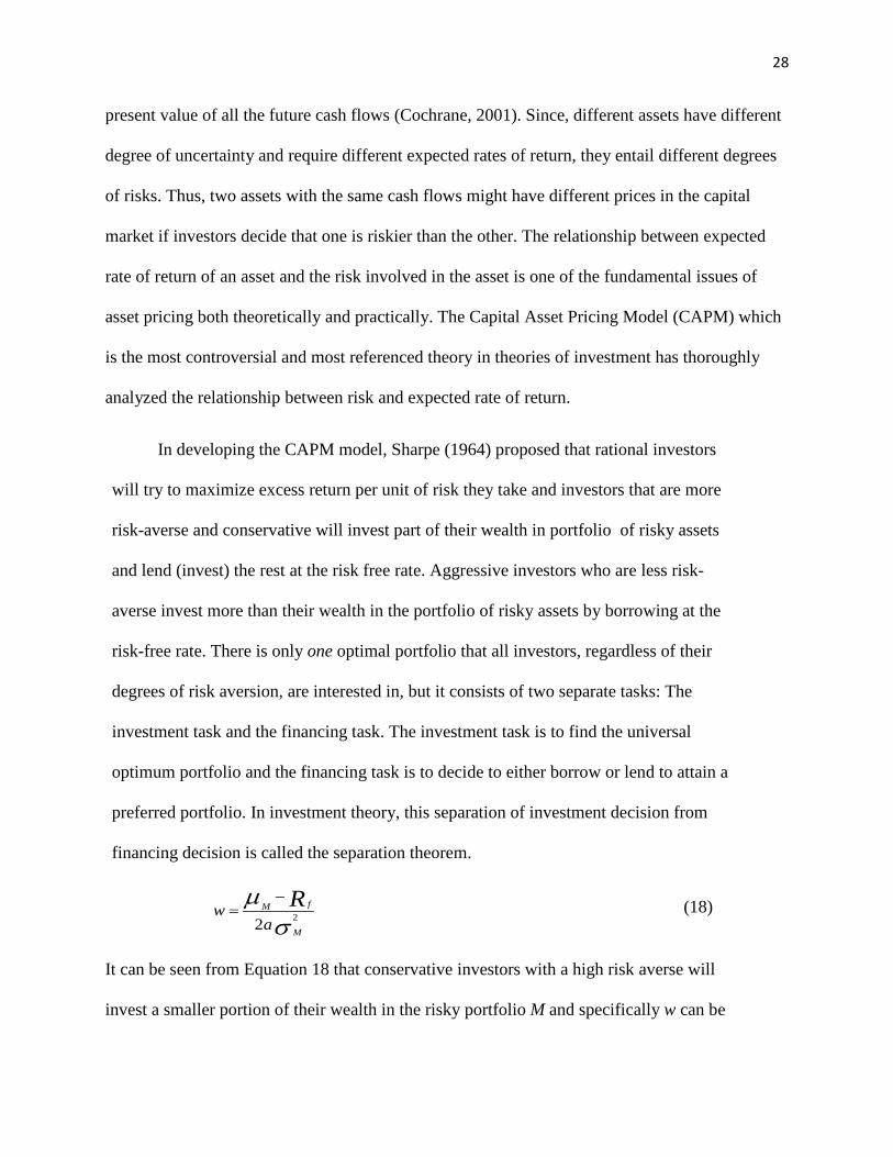
In developing the CAPM model, Sharpe (1964) proposed that rational investors

will try to maximize excess return per unit of risk they take and investors that are more

risk-averse and conservative will invest part of their wealth in portfolio of risky assets

and lend (invest) the rest at the risk free rate. Aggressive investors who are less risk-

averse invest more than their wealth in the portfolio of risky assets by borrowing at the

risk-free rate. There is only one optimal portfolio that all investors, regardless of their

degrees of risk aversion, are interested in, but it consists of two separate tasks: The

investment task and the financing task. The investment task is to find the universal

optimum portfolio and the financing task is to decide to either borrow or lend to attain a

preferred portfolio. In investment theory, this separation of investment decision from

financing decision is called the separation theorem.

σ

µ22 M

fM

aw R−= (18)

It can be seen from Equation 18 that conservative investors with a high risk averse will

invest a smaller portion of their wealth in the risky portfolio M and specifically w can be

29

smaller or greater than 100% depending on the degree of a specific investor’s risk

aversion a.

The Arbitrage Pricing Theory

The Arbitrage Pricing Theory (APT) was first proposed by Stephen Ross in 1976

as an alternative model of asset pricing in the capital market challenging the CAPM

assumptions and conclusions. The APT model is based on the notion of arbitrage in

economic activity and the role of arbitrage in maintaining equilibrium in the markets. In

economic theory, arbitrage is defined as the possibility of making a sure profit without

taking any risk with zero investment. This possibility arises when the law of one price is

violated; meaning that an item trades for different prices in different markets at the same

time or if the item is mispriced in the market. If such an arbitrage opportunity comes up

in the capital market, then the arbitrageur will construct a risk-free portfolio by selling

short the overpriced security (or borrow at the risk-free rate which is the same thing as

selling short the risk-free asset) and buying the underpriced security with the proceed,

thus, make a sure profit with no owned investment.

The critical implication of this risk-free arbitrage portfolio is that any investor,

regardless of risk aversion or wealth, will want to take an infinite position in it and make

infinite profits. Because of these large positions it takes only a few arbitrageurs to force

security prices to move up and down until the arbitrage opportunity is vanished and

equilibrium in the market is restored. This is the core difference between APT

explanation of equilibrium asset prices and that of CAPM. The CAPM argues that all or a

sufficiently large number of investors hold mean-variance efficient portfolios. If some

securities are mispriced in the market, in the sense that their expected returns do not

30

reflect their expected risks as stipulated in Equation 22 above, then a large number of

investors will tilt their portfolios away from the overpriced securities and toward the

underpriced ones. Equilibrium prices in CAPM model is the result of small shifts in the

portfolios of many mean-variance efficient investors. In contrast, the APT model makes

no assumption about investors being mean-variance portfolio holders and it does not

require the actions of many investors to restore equilibrium prices in the capital market.

The no-arbitrage condition of APT states that even relatively few investors are enough to

identify an arbitrage opportunity, mobilize large dollar amounts to take advantage of it,

and exert pressure on the prices to restore equilibrium (Cochrane, 2001).

According to APT model any deviation from equilibrium prices in the capital

market is short-term and the working of arbitrage ensures return to equilibrium. But what

are those equilibrium prices and how are they determined? The answer to this is similar

to that of the CAPM model, that is, for every security investors expect a specific rate of

return from the security and then discount the expected pay-off from the security at that

expected or required rate of return to arrive at the equilibrium price of the security. So,

like in CAPM, the problem of equilibrium price determination in the APT model leads to

the problem of how investors form their expectations with regard to the rate of return that

they require from securities.

The APT model, like CAPM, is an expected return-beta relationship model. But unlike

CAPM that condenses all systematic risks of securities into only one source, the unobservable

market portfolio, the APT argues that any number of macroeconomic factors could be the

common source for systematic risks for all securities’ return. In this way, the APT model

overcomes a major practical problem of CAPM, that of finding a suitable proxy for the market

31

portfolio. Thus, any index that CAPM employs as a proxy for the market portfolio can be

incorporated, if needed, as one of the relevant factors in the APT model without requiring the

index to be a mean-variance efficient portfolio. The common macroeconomic factors in APT

model that affect all securities could be the growth of GNP, inflation rate, exchange rates,

interest rate spreads, and so on. Each security shows a different response to these factors and

therefore for each security investors require distinct compensations for being exposed to each of

these factors. Obviously not all security prices are affected similarly by the factors envisaged in

the APT model. When interest rates change the price of interest sensitive stocks, like stocks of

banks or utility companies, are affected more than the stocks of technology companies. Or, when

the rate of growth of GDP slows, the stock of cyclical companies, like consumer durables or

hotels, are more severely affected than the stock of drug companies.

The relationship between the actual rate of return and the expected rate of return of security i at

time t would then be:

Rit = E (Ri)+ eit (19)

In general, according to APT, in order to invest in a security an investor should be compensated

for all risks arising from the common factors affecting security returns. The risks not related to

common factors are specific to the security and can be diversified away and thus the investors do

not seek compensation for them. Moreover, if actual return of a security deviates from its

expected return the process of arbitrage will quickly eliminate this deviation by putting pressure

on the security’s market price and thereby brings the actual return in line with the expected

return (Reilly and Brown, 1997).

32

Conclusions

The way that firms approach their capital expenditures, what criteria they use in selecting

a project or ranking a series of project, and which project will add value to their shareholders

wealth with the constraint of limited investment funds was discussed in this paper. The best

metrics for evaluation of wealth of the company and selection of the best project was explained

and it was shown that NPV was and the most used and the most efficient metrics for project

evaluation, specifically in large firms.

With respect to the capital structure, the propositions by Modigliani & Miller, was

discussed and it was shown that their theory, though very solid, do not include all relevant

factors into the model such as taxes or solvency cost. The corporate finance theories with respect

to capital structure should develop a theory that proposes an optimal capital structure where the

firm value is maximized and the weighted average cost of capital is minimized. On the dividend

policy theories, there are controversial views: One argument is in favor of irrelevance theory in

which dividend policy of the firms has no effect on the company’s shares valuation. On the other

hand, there is the relevance theory of dividend policy which is divided into two opposing

propositions. The bird-in-the-hand approach that proposes shareholders want assurance and

prefer current cash dividends to uncertain future capital gains and therefore, firms will add value

to their shares by distributing more dividends to the shareholders. The income tax approach that

argues due to the fact that tax rates on dividends are higher than tax rate on capital gains, the

shareholders prefer the future capital gain to the current dividend.

Modern Investment Theories started with Markowitz (1952) paper on portfolio selection

theory. Markowitz suggested that as long as the rates of returns of securities are not perfectly and

positively correlated to the portfolio, the total risk for investment in the portfolio of assets can be

33

reduced through diversification. Furthermore, Markowitz proved, mathematically, that out of all

feasible portfolios that can be constructed from the universe of risky assets, there are some

portfolios that embody minimum risk for a specific level of expected return, and the set of all

such portfolios form a hyperbola called minimum variance frontier. The upper part of minimum

variance frontier represents portfolios that have the highest expected returns for the same level of

risk and is called the mean variance efficient portfolios or the efficient frontier. Markowitz posits

that all rational investors select or should select portfolios from the efficient frontier depending on

their degree of risk aversion.

On the other side of the spectrum, the theory of capital asset pricing model (CAPM) that

was developed by Sharpe in 1964 attempt to guide investors to build a portfolio of different

assets by the way that assets are priced in the capital market. The CAPM was in fact an extension

of Markowitz model, but CAPM introduced the risk-free asset into the model; that is, investors

can lend and borrow money at the fixed risk-free rate in the market. Therefore, according to

CAPM, rational investors seek a portfolio that yields the highest expected return in excess of the

risk-free rate per unit of risk taken. Further, the arbitrage pricing theory (APT) that was fostered

by Ross in 1976 developed an asset pricing model that has less assumptions than CAPM and

considering more risk factors into the model. The APT is a multi-factor expected return-beta

model in which the expected return of any security is a linear function of risk premiums of

various factors and the security’s return responsiveness to those factors. According to APT

model if asset prices deviate from what is implied by their expected return-beta relationships,

then large portfolio adjustment of a few arbitrageurs will restore prices to their equilibrium

levels.

34

Perhaps the simplicity of CAPM is one of the reasons that it is the most talk about in all

the literature on the topic of investment theories. It simply explains that there is a linear

relationship between the expected rate of return of an asset and the risk involved in that asset.

Therefore, on the basis of this return- risk relationship, investors first form their view on the

expected rate of return that they desire to get from an asset and then discount the future expected

pay-offs from that asset at that expected rate of return. Then, if the market price of an asset is

more (less) than that discounted (required rate) they sell (buy) the asset in the market until its

price equates the discounted value. Thus, the capital asset market will be at equilibrium when all

assets trade at prices that reflect the discounted value of their expected future pay-offs.

Therefore, the asset prices equilibrium in the capital market, is reduced to explaining how

investors form their expectations or requirements with respect to the rates of returns of the assets.

Sharpe (1964) then concludes that there is one optimal portfolio for all investors which

encompass all risky assets weighted by their market capitalization and labeled the market

portfolio.

From here, the famous expected return-beta relationship of CAPM is deduced according

to which the expected excess return of any security is linearly related to the beta of the security

and the expected excess return on the market portfolio. The expected return-beta relationship is

the basis of equilibrium asset prices in the capital market and if any deviation from equilibrium

prices occur in the market the mean variance efficient investors acting on the basis of expected

return-beta relationship will readjust their portfolios and restore equilibrium prices. The analysis

and explanation of CAPM both theoretically and empirically will be discussed in another paper.

Referrences

35

Benninga, S. (2000). Financial modeling. Cambridge, MA: The MIT Press.

Bodie, Z., Kane, A. & Marcus, A. J.1993). Investments. Boston, MA: Richard D. Irwin,

Inc.

Brealy, R. A., Myers, S. C., & Marcus, A. J. (2004). Fundamentals of corporate finance New

York: McGraw-Hill Irwin.

Cochrane, J. (2001). Asset pricing. Princeton, NJ: Princeton University Press.

Gitman, L. J. (2000). Principles of managerial finance. New York: Addison Wesley.

Gordon, M. J. (1989). Corporate finance under MM theorems. Financial Management, 2, 19-28.

Graham, J. R. & Harvey, C. R. (2001). The theory and practice of corporate finance: Evidence

from the field. Journal of Financial Economics, 60, 187-243.

Graham, J. R. & Harvey, C. R. (2002). How do CFOs make capital budgeting and capital

structure decisions? Journal of Applied Corporate Finance, 15, 1-28.

Haugen, R. A. (2001). Modern investment theory. Upper Saddle River, NJ: Prentice Hall.

Markowitz, H. M. (1952). Portfolio selection. Journal of Finance, 7, 77-91.

Modigliani, F. & Miller, M. H. (1961). Dividend policy, growth, and valuation of shares. Journal

of Business, 34, 411-433.

36

Modigliani, F. & Miller, M. H. (1963). Corporate income taxes and the cost of capital: A

correction. American Economic Review, 53, 433-43.

Reilly, F. K. & Brown, K. C. (1997). Investment analysis and portfolio management. New

York: The Dryden Press.

Ross, S.A. (1976). The arbitrage theory of capital asset pricing. Journal of Economic Theory,13,

341-360

Ross, S. A., Westerfield, R. W., & Jordan, B. D. (2001). Essentials of corporate finance. New

York: McGraw-Hill Irwin.

Sharpe, W. F. (1964). Capital Asset Prices: A Theory of market equilibrium under conditions of

risk. Journal of Finance, 19, 425-442.