similarity analjysis of d~erential equations by lie group - deep blue
TRANSCRIPT
Similarity AnalJysis of D~erential Equations
by Lie Group
!IJ TSUNG Y. NA
Department of Mechanical Engineering The University of Michigan, Dearborn Campus Dearborn, Michigan
UTZd ARTHUR G. HANSEN
Purdue University, West Lafayette, Indiana
ABSTRACT: Methods for transforming partial differential equations into forms more
suitable for analysis and solution are investigated. The idea of Lie’s infinitesimal contact
transformation group is introduced to develop a systematic method which involves mostly
algebraic manipulations. A thorough presentation of the application of this general method
to the problem of similarity analyses in a broader sense-namely, the similarity between
partial and ordinary differential equations, boundary value and initial value problems,
and nonlinear and linear equationsis given with new and very general methods evolved
for deriving the possible groups of transformations.
1. Introduction
The investigations to be presented in this paper are an outgrowth of a continuing study of ways in which partial differential equations associated with problems of physical interest may be simplified through transformation of independent and dependent variables (14). As the investigation proceeded, certain facts became clear. First it was noted that the usual types of trans- formation for simplifying partial differential equations of physical problems were usually of a rather special class. This led to the question of possibly generalizing the class of transformations noted. A second area of investigation centered on broadening the definition of similarity to include other trans- formations which change a given problem into a simpler problem in some sense or other, instead of the usual interpretation of similarity which implies simply a reduction in the number of variables of a given problem.
It has been known for some time that (5-7) the theory of continuous transformation groups gives promise of providing a very general method of analysis. The method is by no means new. In fact, the basic ideas date back to the last century and are found in the work of the mathematician Sophus Lie. Moreover, the theory of groups has been applied quite extensively in recent times by investigators in the field of similarity analysis. Nevertheless, there still exists a need for a truly in depth study of the application of Lie’s theory to the similarity analysis of problems other than the reduction of the
471

Tsurzg Y. Na and Arthur G. Hansen
number of variables in a partial differential equation (8-10). It therefore seemed reasonable to find how far Lie’s ideas might be pursued in formu- lating a very general approach to similarity analyses.
The theory of continuous groups was first applied to the solution of partial differential equations by Birkhoff (5) who used a one-parameter group. Morgan (6) proved a theorem which established the condition under which the number of variables can be reduced by one. Morgan’s theorem was later extended by Michal (11) to similarity transformations which reduce the number of independent variables by more than one.
One of the difliculties of the approach by Birkhoff and Morgan is that it is based on particular given groups of transformations. To begin with, a group has to be arbitrarily assumed and Morgan’s theorem can then be used to establish whether or not the differential equation transforms conformally under this particular group. If it does, similarity solutions will then exist and the similarity variables can then be taken as the functionally independent invariants of this group. The question which remains is whether or not there are other groups under which similarity solutions exist.
In this paper, the idea of Lie’s infinitesimal contact transformation groups is applied to develop a method for searching possible groups of transformations, instead of arbitrarily assuming one at the outset.? The method is then applied to a broader class of similarity analyses: namely, the similarity between partial and ordinary differential equations, boundary and initial value problems and nonlinear and linear differential equations.
ZZ. The Znjinitesimal Transformation
A group is said to be continuous if, between any two operations of the group, a series of operations within the group can always be found of which the effect of any operation in the series differs from the effect of its previous operation only infinitesimally. The concept of infinitesimal transformations comes as a natural consequence of the definition of a continuous transfor- mation group. An infinitesimal transformation is one whose effects differ infinitesimally from the identical transformation. Thus, any transformation of a finit’e continuous transformation group which contains the identical transformation can be obtained by infinite repetition of an infinitesimal transformation.
Let the identical transformation be
x1 = +(x2 9, a& = x; y1 = (x2 y, a,) = y, (1)
where a,, is a particular value of the general parameter a. Then the trans- formation
x1 = +(z, Y, a0 + aa), y1 = #(x, Y, a0 + 84, (2) t An alternative approach based on an extended Morgan’s method in searching for
possible groups of transformations has recently been developed by Moran et al. (12) which starts from a slightly less general transformation than the contact transformation. It has also been applied to various types of problems, among which are the reduction of differential equations to algebraic equations (13) and its application to dimensional analysis (14).
472 Journal of The Franklin Institute
Similarity Analysis of Differential Equations by Lie Group
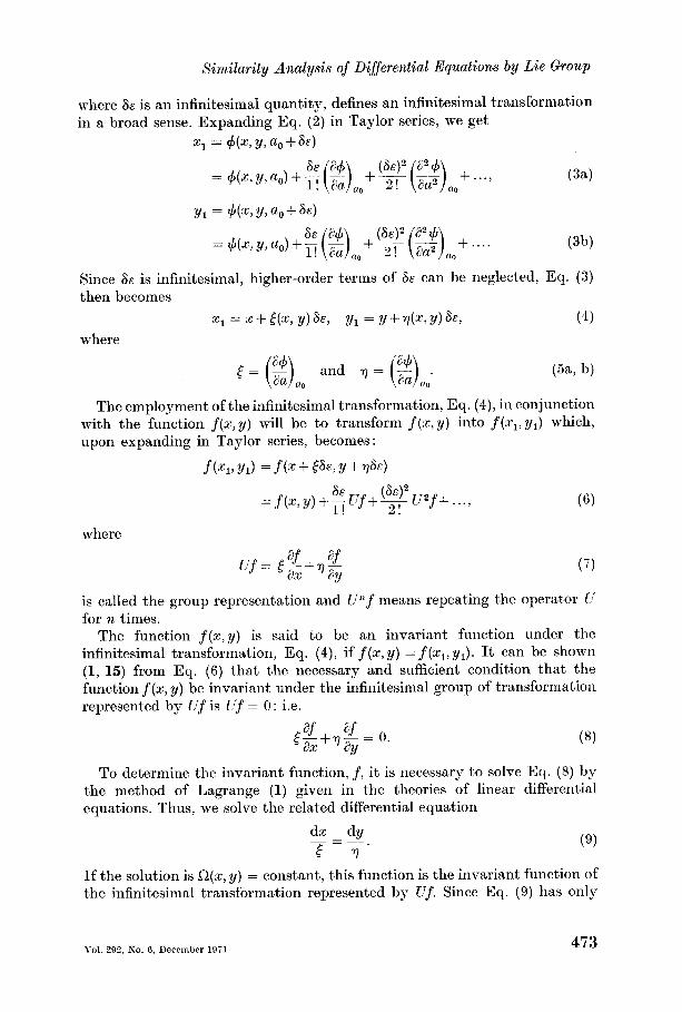
where & is an infinitesimal quantity, defines an infinitesimal transformation in a broad sense. Expanding Eq. (2) in Taylor series, we get
Xl = $G, y>%l+w
= ~(x,y,ao)+~(~),,+~(~),,,+...~
= l~(x,y,ao)+~~).,+~~)..+...
Pa)
(3b)
Since 8~ is infinitesimal, higher-order terms of 6e can be neglected, Eq. (3) then becomes
where
1:1=x+&2, y)6e, y1= y+&Gy)h (4)
a#J 5= (-) aa ao
(53, b)
The employment of the infinitesimal transformation, Eq. (4), in conjunction with the function f(x, y) will be to transform f(z, y) into f(zl, yJ which, upon expanding in Taylor series, becomes:
f(x.1, YJ =f(x+@%y+$&)
=f(x,y)+%f+wPf+ . l! 2! ..’
where
af af u.f = 5,+7:y
is called the group representation and U’lf means repeating the operator U for 12 times.
The function f(x, y) is said t.o be an invariant function under the infinitesimal transformation, Eq. (4), if f(~, y) =f(xl, yJ. It can be shown (1, 15) from Eq. (6) that the necessary and sufficient condit,ion that the function f(~, y) be invariant under the infinitesimal group of transformation represented by Uf is Uf = 0: i.e.
(8)
To determine t’he invariant function, f, it is necessary to solve Eq. (8) by the method of Lagrange (1) given in the theories of linear differential equations. Thus, we solve the related differential equation
dx dy
r=7 (9)
If the solution is Q(x, y) = constant, this function is the invariant function of the infinitesimal transformation represented by Uf. Since Eq. (9) has only
Vol. 292,No. 6, Dec~mbcr 1971 473

Tsung Y. Na and Arthur G. Hansen
one independent solution depending on a single arbitrary constant, a one- parameter group in two variables has one and only one independent invariant.
In the case of n variables, all the theories corresponding to two variables can be generalized by following the same pattern. For example, if a function of n variables f(x,, . . ., x,J is invariant under the infinitesimal transformation
z; = Xi-t&(Z, )...) X,)8& (i = l)...) n) (10)
then a necessary and sufficient condition is again Uf = 0 which, in its expanded form, is
&(x1 )...) x,)-ig+...+&(xl ,..., xg = 0. n
(11)
Following the same reasoning as in two-dimensional case, the invariant functions can be obtained by integrating the following equations:
dx _A=dx, =.,.= !!j%. 51 52
(12)
n
Since there are (n- 1) independent solutions to Eq. (12) a one-parameter group in n variables has (n- 1) independent invariants. The invariant functions are therefore
a,(~,, . . . . xn) = c,, m = 1, . . . . (n- l), (13)
and are the solutions to the system of equations given by Eq. (12).
III. Differential Equations Admitting a Given Group of Transformations
Consider now a function
F = F x1, . . . . x,; yl, . . . . y,; . . . . ~ (14)
the arguments of which, assumed 1, in number, contain derivatives of yi up to order Ic. Such a function is known as a differential form of the kth order in m independent variables (7). Designate the arguments by zr, . . . . zP, e.g.
21 = Xl, .z2 = x2, . . ..Z._l = akY?L akY?l
a(xm-l)k ’ %=ao”’
Eq. (14) can be written in a simpler form as F = F(z,, . . . . zp) which is said to admit of a given group represented by
Uf = &(Zl,..., zp)g+...+&&l )...) zp,g 1 P
(15)
if it is invariant under this group of transformation. Therefore, the function F admits of a group if UF = 0, or
g+...+g= 0. 1 P
474
(16)
Journal of The Franklin Institute

Similarity Analysis of Differential Equations by Lie Group
It was shown in the preceding article that there are (p - 1) functionally independent solutions, or invariants, to this equation, namely,
rlrn = SZm(zl, . . . . x9) = constant, m = 1, . . . . (p- 1). (17)
An important theorem will be quoted here without proof (1). Based on this theorem, if a differential equation F(z,, . . . . zP) = 0 is invariant under the infinitesimal transformation, it must be expressible in term of the (p - 1) functionally independent invariants. Thus, we write
F(z 1, . ..> zp) = CC,,, . . . . qp_J = 0, (18) where the 7’s are given by Eq. (17).
For a given group of transformations, the transformation functions, ti, in Eq. (10) are known functions. In the original group-theoretic method developed by Birkhoff (5), and Morgan (6), two groups, namely, the linear and the spiral groups, were considered. For the linear group, fi = Cixi (; = 1 , . . . ,p) whereas for the spiral group e, = C, and ti = Ci zi (i = 2, . . . , p). The theories outlined above are enough for the determination of possible similarity transformations (1). The similarity transformations thus obtained, however, correspond only to the two particular groups of transformations. Since there is no proof that these two groups are the only two possible for similarity solutions to exist for a given partial differential equation, it is still necessary to raise the question: Given a partial differential equation, what are all possible groups of transformations that make similarity solution possible? In other words, are there other groups other than the linear or the spiral groups 1
To answer questions of this kind, we shall develop a systematic procedure in searching for all possible groups of transformations by using Lie’s theories of infinitesimal contact transformation groups. Although the concepts were introduced by Lie in the latter part of the nineteenth century, its significance in the solution of nonlinear differential equations has not been fully explored.
IV. Contact Transformations
Before entering into discussion of the contact transformations, the concept of an extended group has to be introduced. Consider the one-parameter group of transformation :
x1 = d(x,y,a), y1 = #(x,y,a). (19)
Suppose y is regarded as a function of x, then if the differential coefficient p ( = dyldx) be considered as a third variable, it will be transformed to pl by
p1 _ 2 _ (WW + (way) P 1 (a+/ax) + (&@y)p = x(z7 yyp3 a)* (20)
For the infinitesimal transformation defined by Eq. (4), the transformed coefficient pr can be shown to be
PI = P+$(x,Y>P)> (21)
Vol. 292, No. 6, December 1971 475
Tsung Y. Na and Arthur G. Hansen
where
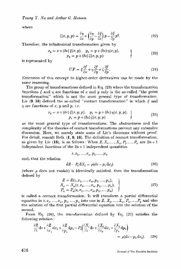
S(X,Y,P) = g+(gj-z)P-gP?
Therefore, the infinitesimal transformation given by
Xl = x + (a&) 5(x, Y), Yl = Y + (a&) ?1(x, Y),
Pl = P + (W 5(x, Y> P) is represented by
(23)
(24)
Extension of this concept to higher-order derivatives can be made by the same reasoning.
The group of transformations defined in Eq. (23) where the transformation functions .$ and 77 are functions of x and y only is the so-called “the point transformation” which is not the most general type of transformation. Lie (9, 16) defined the so-called “contact transformation” in which E and 71 are functions of x, y and p, i.e.
Xl = x+(~E)&,Y,P), Yl = Y+(~&)q(X,Y,P), \
Pl = P + (a&) 5(X> Y, P) j (25)
as the most general type of transformations. The abstractness and the complexity of the theories of contact transformations prevent any extensive discussion. Here, we merely state some of Lie’s theorems without proof. For detail, consult Refs. (1, 9, 16). The definition of contact transformation, as given by Lie (16), is as follows : When 2, Xi, . . . , X,, PI, . . . , P, are 212 + 1
independent functions of the 2n + 1 independent quantities
.%x1, . . ..&.P1, . . ..Pn.
such that the relation
dZ - Pi dXj = p(dz -pi dxi) (26)
(where p does not vanish) is identically satisfied, then the transformation defined by
2 =-&xi, . . ..%.Pl, . . ..P.),
-q = &(%X1, . . ..X.,Pl, . . ..P.), (27)
p, = p,(Z,Xl, . . ..X.,Pl, . . ..P.) 1
is called a contact transformation. It will transform a partial differential equation in x, x1, . . ., x,, pl, . . . ,pn into one in 8, X,, . . ., X,, PI, . . . , P, and also the solution of the first partial differential equation into the solution of the second.
From Eq. (26), the transformation defined by Eq. (27) satisfies the following relation :
= p(dz-pidxi). (28)
476 Jourrml of The Franklin Institute

Xiwdarity Analysis of Differential Equations by Lie Group
For the infinitesimal transformation
.z = s + (W 0% zg, P,), xi = xi + (84 &, z/o P,),
pi = P’i + (SE) n&, z/o P/J, I (29)
we get:
If a characteristic function, W, is defined as W = pi fi - 5, then Eq. (39) gives
aw aw “r = -az,-Prz. (3h b, c)
To get the transformation functions for higher-order derivatives, we consider the transformation defined by Eq. (29), adding the following higher-order terms :
and q, = Pjr, + (6s) ~j,&, xp Pp P,,,) (32)
<kl = Pjkl + (SE) .rri& xp> P/L> Pps P,,).
By definition, we write
(33)
which, upon substitution and (33) and subtracting
dP, = &dX, (34)
of the infinitesimal transformation, Eqs. (29), (32) the quantity +psikdx, from both sides, gives
d njk = G (rk - Pjk fj) (35)
or, in terms of fj and z-~,
(36)
To express irjk in terms of the characteristic function W, it is necessary to put expressions for rk and ci from Eq. (31) into Eq. (36).
Similarly, for the third-order function rjkl, we get
d
or
(38)
Vol. 292, Ko. 6, Decenrbrr 1071 477

Tsung Y. Na and Arthur G. Hansen
In order to express njkl in terms of the characteristic function W, we have to express njk and 6 in terms of W, as in Eqs. (31) and (36), and substitute into Eq. (38).
V. Similarity Analysis of the Difusion Equation
As an illustration of the method of searching for possible groups of trans- formations, let us consider the diffusion equation,
au a2u ~-“w = O* (39)
The infinitesimal contact transformation defined by Eqs. (29), (32) and (33)
is now introduced where x, x1 and x2 are replaced by u, t and y respectively. Also, the following notations are used:
au au azu a2u P=,,, q=,,, P22=r2’ Plz=;;tY’ etc.
dY (40)
The transformation functions 5, ti, rr’i and rjk can be expressed in terms of the characteristic function W as shown in Eqs. (31) and (36).
It was shown that the necessary and sufficient condition that a partial differential equation F(t, y, u,p, q,p12,pz2) = 0 be invariant under the group of transformations represented by Uf is UF = 0 which for the diffusion equation, is
(41)
where the parentheses represents the differential equation (p - vpS2). Carrying out the operation in Eq. (41) and substituting expressions from Eqs. (31) and (36) into Eq. (41) yields
or
rri-vrr22 = 0
_~!&p!!!+ a2 w v-++vq
aY2 &T+vq2g
a2 w + 2P12 wp v + 21712 P
a2 w a2w a2w --v+2p- au ap a~ aq
+Pq- au aq
(42)
a2 w +‘PT2 ap2
a2w p2a2w aw -+2P,2P~q+~ ap2+1)7g = 0. (43)
Equation (43) is seen to be a linear partial differential equation in W. Since W is not a function of pi2, the coefficients of the terms involving
p12 and p:2 should be zero. By putting the coefficients of pt2 to zero, the characteristic function W is seen to be a linear function of p, i.e.
w = K(G y, % q) +pw, y, u, PI.
478 Journal of The Franklin Institute
Similarity Analysis of Differential Equations by Lie Group
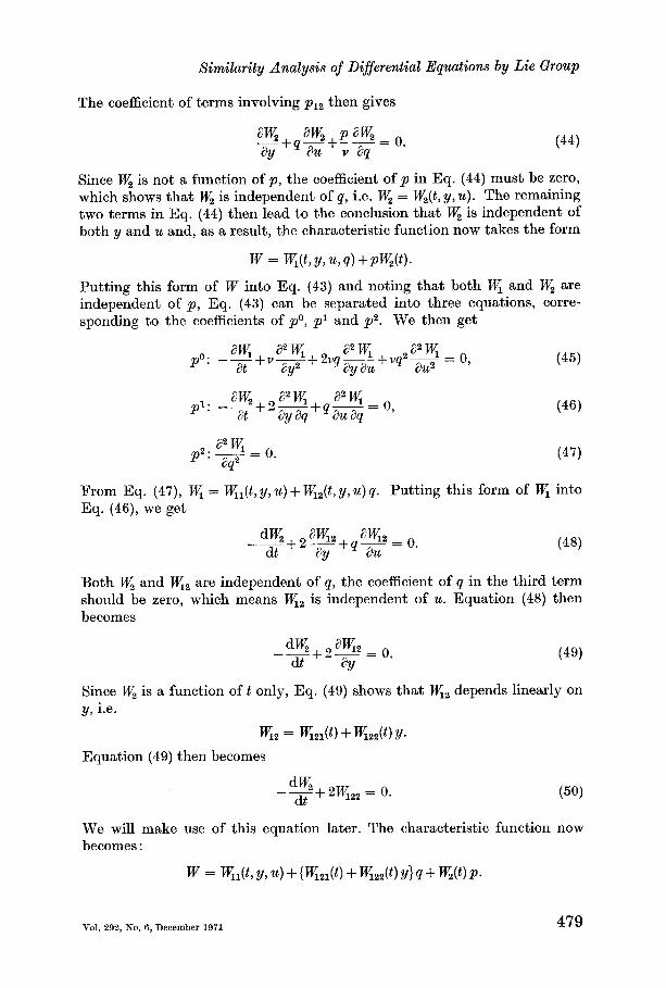
The coefficient of terms involving p12 then gives
8% aw, P aw, -+qa,+-- = 0. ay v aq
(44)
Since W, is not a function of p, the coefhcient of p in Eq. (44) must be zero, which shows that W, is independent of q, i.e. W, = Wz(t, y, u). The remaining two terms in Eq. (44) then lead to the conclusion that W, is independent of both y and u and, as a result, the characteristic function now takes the form
w = WV, Y, u, P) +pW).
Putting this form of W into Eq. (43) and noting that both WI and W, are
independent of p, Eq. (43) can be separated into three equations, corre- sponding to the coefficients of pO, p1 and pa. We then get
P aw aq azw,
0: -L+ v-+ 2vqp at a2y 28% 0
ayau+‘q -&!F= ’
pl: -$+2_ a2 w, a2 w, o ayaq+q&+a4 ’
2. a2w, 0 P-F= *
(45)
(46)
(47)
From Eq. (47), WI = Wll(t, y, u) + WI&t, y, u) q. Putting this form of W, into Eq. (46), we get
_~+2!%+q~ = 0.
aY (43)
Both W, and W,, are independent of q, the coefficient of q in the third term should be zero, which means WI, is independent of U. Equation (48) then becomes
(49)
Since W, is a function oft only, Eq. (49) shows that WI, depends linearly on y, i.e.
w,, = K,,,(t) + W‘&?(t) Ye
Equation (49) then becomes
7
-$+2w1,, = 0.
We will make use of this equation later. The characteristic function now becomes :
w = %(t> YF u) + V%(t) + K2&) Y)4 + K(t) P*
Vol. 292, No. 6, December 1971 479
Tsung Y. iVa and Arthur G. Hansen
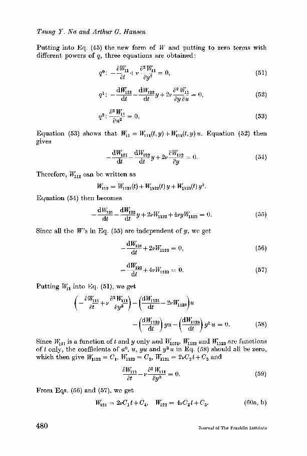
Putting into Eq. (45) the new form of W and putting to zero terms with different powers of q, three equations are obtained:
dKz1 d%, ql: - & ----&-y+22v-- = a2 w,, o
i?y au )
2. a2w,1 o
4.T=.
(51)
(52)
(53)
Equation (53) shows that W,, = Wlll(t, y) + Wllz(t, y) u. Equation (52) then gives
----dty+2V--- = d% d&22 W12 o
dt aY . (54)
Therefore, W,,, can be written as
w,,, = wlzl(t) + w122w Y + %23(t) Y2.
Equation (54) then becomes
dK2, W,, - - - 7 y + 2vq122 + 4Vy&;,,, = 0. dt
Since all the W’s in Eq. (55) are independent of y, we get
dK2, - - + 2vw,,,, = 0,
dt
dW,22 - 7 + 4vw,,,, = 0.
(55)
(56)
(57)
Putting W,, into Eq. (51), we get
Since WI,, is a function oft and y only and W1121, WI,,, and Fhr,, are functions of t only, the coefficients of u,O, u, ye and y2u in Eq. (58) should all be zero, which then give WI,,, = C,, WI,,, = C,, II& = 2vC,t + C, and
Wll a2 Kll 0
-Fat-“-=. @J2 (59)
From Eqs. (56) and (57), we get
w,,, = 2vc1 t + c,, w,,, = 4vc2 t + c,. (6% b)
480 Journal of The Franklin Institute

Similarity Analysis of DiSferential Equations by Lie Group
Also, from Eq. (50), Wz = 4vC, t2 + 2C, t + C,. The final form of the charact’er- istic function is therefore
wt,y,%p,q) = ~~‘,,,(t,y)+{2vC,t+C,+C,Y+C,Y2}U
+ {%‘c, t + c, + (4Vc, t + c,) y} q
+ {4VCz t2 + 2c, t + C,}p,
where Wlll(t, y) is any function satisfying
(61)
(62)
With the characteristic function W obt,ained as in Eq. (61), we now make use of the general theory to find the absolute invariant,s. From Eq. (12), the following relations are obtained :
dt dy du
r=7=7 (63)
where the transformation functions [, 7 and < can be obtained by putting into Eqs. (31) and (36) the characteristic function W given in Eq. (61). Equation (63) then becomes
dt dY 4vc, t2 + 2c, t + c, 2vcr t + c, + (4vC, t + C,) y
du _~_ ~ - WI&, y) - (2vC2 t + c, + c, y + c, y2) u *
(64)
The number of possible groups are large, due to the fact that all C’s are arbitrary and Wlll(t, y) is an arbitrary function satisfying Eq. (62). However, a few special cases of the transformations are given in Table I, together with the transformed differential equations.
TABLE I
Sample solutions of the diffusion equation
Constants Similarity variables Transformed equation
w,,, = 0 7 = Y/h f(T) = u/t” vf” = clf-~7)f’ c, = c, = c, = c, = 0 WI, = 0 17 = Y, f(7) = ulexp (fit) vf”-/3f = 0 c, = c, = c, = c, = 0 %I = 0 q = Y-C,/C,G vf”+ (c,/c,)f’+ (G/C,)f = 0 c, = c, = c, = 0 f = u exp WV&) tl w,,, = 0 17 = Y/t? 7J’f”-T)f’+$f = 0 c, = c, = c, = c, f($ = uy* exp W/+Wl
=c,=o WI,, = val t + Qa, y2 c, = c, = c, = c,
=c,=o
yol. 292, No. 6, December 1971
21 481
Tsung Y. Na and Arthur G. Hansen
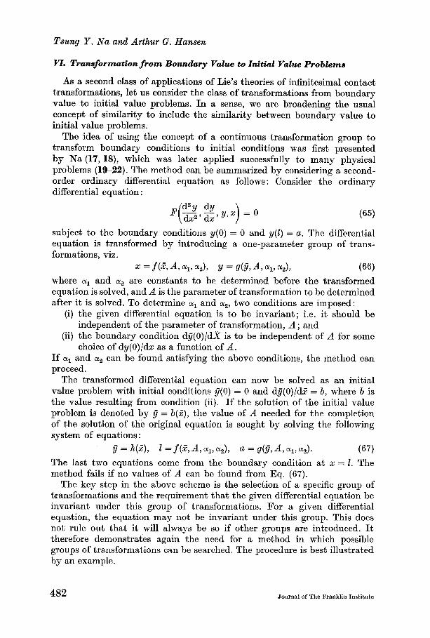
VI. Transformation from Boundary Value to Initial Value Problems
As a second class of applications of Lie’s theories of infinitesimal contact transformations, let us consider the class of transformations from boundary value to initial value problems. In a sense, we are broadening the usual concept of similarity to include the similarity between boundary value to initial value problems.
The idea of using the concept of a continuous transformation group to transform boundary conditions to initial conditions was first presented by Na (17, 18), which was later applied successfully to many physical problems (19-22). The method can be summarized by considering a second- order ordinary differential equation as follows: Consider the ordinary differential equation :
P g,$y,x ( ) =o (65)
subject to the boundary conditions y(0) = 0 and y(Z) = a. The differential equation is transformed by introducing a one-parameter group of trans- formations, viz.
x = f(% A, a1,4, Y = s(s, A, a1,4, (66)
where 01~ and 01~ are constants to be determined before the transformed equation is solved, and A is the parameter of transformation to be determined after it is solved. To determine 01~ and 01~, two conditions are imposed:
(i) the given differential equation is to be invariant; i.e. it should be independent of the parameter of transformation, A; and
(ii) the boundary condition dg(O)/dx is to be independent of A for some choice of dy(O)/dx: as a function of A.
If CQ and 01~ can be found satisfying the above conditions, the method can proceed.
The transformed differential equation can now be solved as an initial value problem with initial conditions g(O) = 0 and dg(O)/db = b, where b is the value resulting from condition (ii). If the solution of the initial value problem is denoted by ?j = b(Z), the value of A needed for the completion of the solution of the original equation is sought by solving the following system of equations :
ii = G% J = ~7% A CQ,~, a = s(B, A, q>+ (‘37)
The last two equations come from the boundary condition at z = 1. The method fails if no values of A can be found from Eq. (67).
The key step in the above scheme is the selection of a specific group of transformations and the requirement that the given differential equation be invariant under this group of transformations. For a given differential equation, the equation may not be invariant under this group. This does not rule out that it will always be so if other groups are introduced. It therefore demonstrates again the need for a method in which possible groups of transformations can be searched. The procedure is best illustrated by an example.
482 Journal of The Franklin Institute

Ximilarity Analysis of Differential Equations by Lie Group
Consider the well-known Falkner-Skan equation in boundary layer theory (23))
F = r+fq+/3(1-p”) = 0 (68)
subject to the boundary conditionsf(0) = p(0) = 0, p(m) = 1 where
p=f’, qzf”) r=f”.
Next, an infinitesimal transformation is defined as:
rl’ = rl + (a&) 5571LL P),
f’ =f+(S&)e(%f>P),
P’ = P + (Se) +?,f, P),
4’ = 4 + (SE) J%f> P, q),
r’ = r + (SC) p(rl,f,p, 4, r), i where, in terms of the characteristic function IV,
(69)
-k = ( x2+2qX$-+q2$+q8 1 ?f w, I I
x3+3qx~~+3q~x~+q~T$+3qx~+3q.- a2 w ) I
(70)
-P = ( af afap
+r 3qz+3XA+a ( ap2 ap af 1
W.
The operator X in Eq. (70) is defined as X = a/aq +p(a/af). The condition for the invariance of Eq. (68), namely, SF/& = 0, or in its expanded form,
~~+e!z$+~~+k~+p~ = 0 (71)
then becomes
A,+A,q+A2q2+A3q3 = 0, (72)
where the variable r in the function p, Eq. (70), was eliminated by using the differential equation, Eq. (68), and the A’s are given by
A, = 2/3pXW-fX2 W-X3 W+/3(1-p”) 3X-+- W, ( ii ix
a2 w A, = (p-3X2+fX)g- W-3x~+3/k?(l-p2$-,
2
A,= 2f$-3X$-,&$
A,=s.
\
j (73)
I
Vol. 292, No. 6, December 1971 483
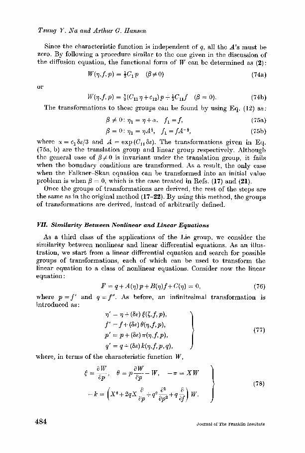
Tsung Y. Na and Arthur G. Hansen
Since the characteristic function is independent of q, all the A’s must be zero. By following a procedure similar to the one given in the discussion of the diffusion equation, the functional form of W can be determined as (2):
Whf,P) = QCIP (B#Oo) (744
or
W(%f, PI = ~(Cllrlf UP + &Lf (B = 0). (74b)
The transformations to these groups can be found by using Eq. (12) as:
P#O:%=71+% &fi=.f, (75a)
,9 = 0: v1 = qA*, fi = fA-*, (75b)
where 01= c1 S&/3 and A = exp (C,, SE). The transformations given in Eq. (75a, b) are the translation group and linear group respectively. Although the general case of /J # 0 is invariant under the translation group, it fails when the boundary condit’ions are transformed. As a result, the only case when the Falkner-Skan equation can be transformed into an initial value problem is when ,f3 = 0, which is the case treated in Refs. (17) and (21).
Once the groups of transformations are derived, the rest of the steps are the same as in the original method (17-22). By using this method, the groups of transformations are derived, instead of arbitrarily defined.
VII. Similarity Between Nonlinear and Linear Equations
As a third class of the applications of the Lie group, we consider the similarity between nonlinear and linear differential equations. As an illus- tration, we start from a linear differential equation and search for possible groups of transformations, each of which can be used to transform the linear equation to a class of nonlinear equations. Consider now the linear equation :
F = s+A(rl)p+%)f+Ch) = 0, (76)
where p = f’ and q = f “. As before, an infinitesimal transformation is introduced as :
7’ = 7 + @&I 5(5Yf, PI>
f’ = f + (W h,fTPL P’ = P + (W 4%f, P),
P’ = P + (Se) %f,zA PL I
(77)
where, in terms of the characteristic function W,
f=f$ e=pg-w, -?T=XW
(78)
-II: = c
x2+2qx$+q2&2+q1 Sf 1
w. 1 484 Journal of The Franklin Institute

Similarity Analysis of Differential Equations by Lie Group
The operator X in Eq. (78) is defined as X = aiZ_rl +p(a/af ). Again, the invariance of Eq. (76) requires that aFj6.z = 0, i.e.
Replacing F by the expression given in Eq. (76), Eq. (79) gives
+ F(AP+B~+C)~ = 0.
(79)
Equation (SO) is the equation which determines the functional form of W. Consider first the case in which the independent variable is not transformed,
i.e. x = 7. From which aW/Zp = 0. In other words, W is independent of p. By following the same reasoning as in the analysis of the diffusion equation, it can be proved (3) that the characterist,ic function W is given by
W(%f) = K(r)+f%
where W, and W, satisfy the equation:
(81)
d2Wl ~+&)~+B(~) w, = w~c(~). (82)
This is an ordinary linear differential equation for t,he solution of W,. It call be solved if A, B and C are given.
Consider the case in which 1% = 0 and C = 0. For this case, Eq. (82) is obviously satisfied and the characteristic function becomes: W = f W,. The invariances can be solved by
drl df dI, -= -w2f=-w,p> 0
which gives 7 = constant and p/f = constant. The new variables are therefore
x=7, y,L.fl. f f
(83)
As an example, the well-known generalized Riccati’s equation
y’+P(x) y+&(x) y2 = R(x) (84)
can be cited. It was shown by Riccati (15) that a transformation y = f’/Qf
Vol. 292, No. 13, December 1071 485
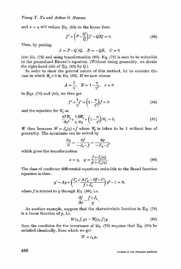
Tsung Y. Na and Arthur G. Hansen
and x = 77 will reduce Eq. (84) to the linear form
f”+(P-;)f’-QRf = 0. (85)
Thus, by putting
A = P-Q’/&, B = -QR, C = 0
into Eq. (76) and using transformation (SO), Eq. (76) is seen to be reducible to the generalized Riccati’s equation. (Without losing generality, we divide the right-hand side of Eq. (83) by Q.)
In order to show the general nature of this method, let us consider the case in which W, # 0 in Eq. (82). If we now choose
A=:, &I-;, c=O rl 77
in Eqs. (76) and (82), we then get
and the equation for WI as
E!i+E!i+ 1-n w = 0
w rl dr) ( 1 r12 1 ’ (87)
W then becomes W = J,(q) +f where W, is taken to be 1 without loss of generality. The invariants can be solved by
drl df dP -= -----= 0 - Jn-f - J:,-f’
which gives the transformation
a = v7,
The class of nonlinear differential equation is thus:
f +J,(v) y =p+J;($
(88)
equations reducible to the Bessel function
y’-Ay+ )
y2- 1 = 0,
where f is related to y through Eq. (88), i.e.
df f+J,z
G=Y’
As another example, suppose that the characteristic function in Eq. (78) is a linear function of p, i.e.
W(%f,P) = w,(%f)P (89)
then the condition for the invariance of Eq. (76) requires that Eq. (80) be satisfied identically, from which we get
w = tip,
486 Journal of The Franklin Institute
Ximilarity Analysis of Differential Equations by Lie Group
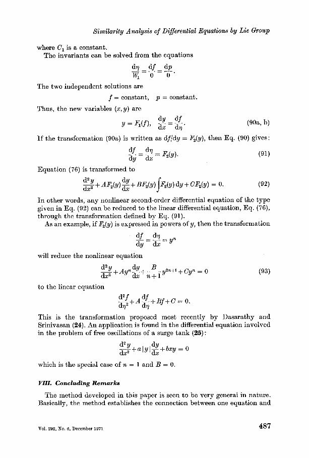
where C, is a constant. The invariants can be solved from the equations
dq df dp -=-=-....-. W, 0 0
The two independent solutions are
f = constant, p = constant.
Thus, the new variables (x, y) are
y = q(f), dy = df . dx dq
(9% b)
If the transformation (90a) is written as dfidy = F!(y), then Eq. (90) gives:
df drl dy = & = -G(Y)-
Equation (76) is transformed to
(91)
In other words, any nonlinear second-order differential equation of the type given in Eq. (92) can be reduced to the linear differential equation, Eq. (76), through the transformation defined by Eq. (91).
As an example, if Fz( y) is expressed in powers of y, then the transformation
df d?
dy=z=yn
will reduce the nonlinear equation
d=y dy B =+Ayn-+ - y2n+1+ Cy" = 0 dx n+l
(93)
to the linear equation
cf+Adf+Bf+C= 0. d? drl
This is the transformation proposed most recently by Dasarathy and Srinivasan (24). An application is found in the differential equation involved in the problem of free oscillations of a surge tank (25):
$$+alyl~+bxy = 0
which is the special case of n = 1 and B = 0.
VIII. Concluding Remarks
The method developed in this paper is seen to be very general in nature. Basically, the method establishes the connection between one equation and
Vol. 292, No. 6, December 1971 487
Tsung Y. Na and Arthur G. Hansen
all other equ&ions under the contact transformation group of transformation,
by the procedure of choosing different forms of the characteristic function W.
It is not therefore merely restricted to the class of similarity analyses where
the number of variables are to be reduced. To reduce the number of variables
by more than one, a multiparameter group must be introduced (4).
Acknowledgements
The authors appreciate the support from NASA Marshall Space Flight Center through a contract (NAS 8-20065). Dr. J. R. Watkins of this Center was very helpful during this work, and therefore we wish to express our appreciation.
References
(1) T. Y. Na, D. E. Abbott and A. G. Hansen, “Similarity analysis of partial differential equations”, Technical Rept., NASA Contract NAS s-20065, Univ. of Michigan, Dearborn Campus, Dearborn, Mich., Mar. 1967.
(2) T. Y. Na and A. G. Hansen, “General group-theoretic transformations from boundary value to initial value equations”, NASA CR-61218, Feb. 1968.
(3) T. Y. Na and A. G. Hansen, “General group-theoretic transformations from nonlinear to linear differential equations”, Proj. Rep. 07457-19-T, Univ. of Michigan, Dearborn, Mich., Apr. 1969.
(4) T. Y. Na and A. G. Hansen, “Similarity solutions of partial differential equations by multiparameter Lie group”, Rep. NASA 8-20065, Univ. of Michigan, Dearborn, Mich., Aug. 1969.
(5) G. Birkhoff, “Hydrodynamics”, Princeton, Princeton Univ. Press, 1950. (6) A. J. A. Morgan, “Reduction by one of the number of independent variables in
some systems of partial differential equations”, Quart. Appl. Math., Vol. 3, 1952. (7) A. G. Hansen, “Similarity Analyses of Boundary Value Problems in Engineering”,
Englewood Cliffs, N.J., Prentice-Hall, 1964. (8) E.-A. von Miiller and K. Matschat, “uber das Auffinden von lihnlichkeitsl&ungen
partieller Differentialgleichungssysteme unter Benutzung von Transformations-
gruppen, mit Anwendungen auf Probleme der StrBmungsphysik”, Berlin, Akademie-Verlag, 1962.
(9) A. Cohen, “An Introduction to the Lie Theory of One-parameter Groups”, New York, Heath, 1917.
(10) G. W. Bluman and J. D. Cole, “General similarity solutions of the heat equation”, 12th Int. Cong. Applied Mechanics, San Francisco, Calif., Apr. 1969.
(11) A. D. Michal, “Differential invariance and invariant partial differential equations under continuous transformation groups in normed linear space”, Proc. natl Acad. Sci. U.S.A., Vol. 37, pp. 623-627, 1952.
(12) M. J. Moran, R. A. Gaggioli and W. B. Scholten, “A new systemmatic formalism for similarity analysis with application to boundary layer flow”, Math. Res. Center Rep. 918, Univ. of Wisconsin, Aug. 1968.
(13) M. J. Moran and R. A. Gaggioli, “On the reduction of differential equations to algebraic equations”, Math. Res. Center Rep. 925, Univ. of Wisconsin, Aug. 1968.
(14) M. J. Moran and R. A. Gaggioli, “A generalization of dimensional analysis”, Math. Res. Center Rep. 927, Sept. 1968.
(15) E. L. Ince, “Ordinary Differential Equations”, New York, Dover, p. 103, 1956. (16) S. Lie, Math. Annalen, Vol. 8, p. 220, 1875. (17) T. Y. Na, “Transforming boundary conditions t,o initial conditions for ordinary
differential equations”, SIAM Review, Vol. 9, pp. 204-210, 1967. (18) T. Y. Na, “Further extension on transforming from boundary value to initial
value problems”, SIAM Review, Vol. 10, 1968.
Joumnl of The Franklin Institute
Similarity Analysis of Differential Equations by Lie Group
(19) T. Y. Na and S. C. Tang, “A method for the solution of heat conduction equation with non-linear heat generation”, ZAMX, Vol. 49, pp. 1-2, pp. 45-52, 1969.
(20) T. Y. Na, “An initial value method for the solution of MHD boundary layer equations”, Aeronaut. Q., Vol. 21, pp. 91-99, Feb. 1970.
(21) T. Y. Na, “An initial value method for the solution of a class of nonlinear equations in fluid mechanics”, J. bus. Engng, Vol. 92, Series D, pp. 503-509, 1970.
(22) H. S. Na and T. Y. Na, “An initial value method for the solution of certain nonlinear equations in biology”, J. Biosci., Vol. 6, pp. 25-35, 1970.
(23) V. M. Falkner and S. W. Skan, “Some approximate solutions of the boundary layer equations”, Phil. Mug., Vol. 12, p. 865, 1931.
(24) B. V. Dasarathy and P. Srinivasan, “Study of a class of nonlinear systems reducible to equivalent linear system”, AIAA Journal, Vol. 6, No. 4, pp. 736-737, Apr. 1968.
(25) N. W. McLachlan, “Engineering applications of nonlinear theory”, in “Proc. of Symp. of Nonlinear Circuit Analysis”, Interscience, New York, 1956.
489