silvah users guide - northern research station · inventory settings ... silvah users guide iv ......
TRANSCRIPT

SILVAH Users Guide

Table Of Contents Welcome to SILVAH ....................................................................................... 1 Forest Management - Decision Support ............................................................. 2 Chapter 1 - SILVAH Overview .......................................................................... 5
Getting Started ........................................................................................... 5 SILVAH Programs........................................................................................ 5 Analysis and Prescription Operating Modes...................................................... 6 Adding Stands Together ............................................................................... 7 System Requirements .................................................................................. 7 Managing Your Files..................................................................................... 8 Keystrokes and Interactive Help .................................................................... 9 Data Entry Layout ......................................................................................10 About the Data Entry Program .....................................................................12 About the Analysis and Prescription Program..................................................13 About the TREECALC program......................................................................14
Chapter 2 - Installing SILVAH On Your Computer...............................................16 Installation Procedure .................................................................................16 Items Installed On Your Computer ................................................................16
Chapter 3 - Data Entry and Manipulation ..........................................................18 Starting a New Stand..................................................................................18 Opening An Existing Data File ......................................................................18 Saving Your Data .......................................................................................18 Converting Data From Older Versions............................................................19 Inventory Settings......................................................................................19 Management Information ............................................................................20 Identification, History and Cover Type...........................................................21 Physiography and Site ................................................................................21 Working With Grid Tables ............................................................................22
About Grid Tables ....................................................................................22 Moving Through The Grid..........................................................................22 Data Entry Shortcuts For the Grid ..............................................................22 Configuring Data Fields On The Grid ...........................................................23 Copying Data From the Grid......................................................................25
Entering Overstory Data..............................................................................25 About Tree and Plot Records .....................................................................25 How to Get Started..................................................................................26 Entering the Data ....................................................................................28 Adding Tree Observations .........................................................................29 Manipulating Plots ...................................................................................29
Entering Understory Data ............................................................................31 About Understory Data.............................................................................31 Entering extended regeneration data..........................................................31 Entering checkmark regeneration data........................................................33
Entering Non-Native Invasive Species ...........................................................34 About Non-Native Invasive Species Data.....................................................34 Entering Plot-based NNIS Observations.......................................................36 Entering Off-plot NNIS Observations ..........................................................37
Chapter 4 - Setting Up a Defaults File ..............................................................39 About SILVAH defaults ................................................................................39 Starting a New Defaults File.........................................................................39 Opening An Existing Defaults File..................................................................39
ii
Table Of Contents
Saving Your Defaults ..................................................................................40 Converting Older Defaults Files.....................................................................40 Calculation Settings ....................................................................................40
Default Management Values......................................................................40 Default Inventory Settings ........................................................................41 Default Commercial Sale Breakpoints .........................................................42 Default Diameters for Volumes ..................................................................43 Default Log Rule and Other Values .............................................................44
System Settings.........................................................................................44 Default Output Folders .............................................................................44 Default Operation Mode............................................................................45
Plant Species Information............................................................................45 About Species Codes................................................................................46 Default Species Codes..............................................................................47 Default Species Parameters.......................................................................48
Chapter 5 - Analysis and Prescription ...............................................................50 Starting Analysis and Prescription.................................................................50 Changing Runtime Options ..........................................................................51 About Interactive Mode ...............................................................................53 About Stand Growth Projection.....................................................................59 Creating a Script File ..................................................................................59 Creating a Batch Job...................................................................................61 Running your data......................................................................................62 Read Alternate Defaults File.........................................................................63 Quitting the Program ..................................................................................63 Viewing Your Output ...................................................................................64
Chapter 6 - TREECALC, A Volume and Value Calculator.......................................65 Starting TREECALC .....................................................................................65 How to Use TREECALC ................................................................................66
Chapter 7 - SILVAH Definitions and References .................................................69 About references........................................................................................69 Volume and Value Calculations.....................................................................71
Merchantable Heights...............................................................................71 Cubic Volumes ........................................................................................72 Board Volumes ........................................................................................72 Net Volumes ...........................................................................................73 About Report Volumes..............................................................................73 Grade ....................................................................................................74 Value.....................................................................................................74
Regeneration .............................................................................................75 Advance Regeneration Guidelines ...............................................................75 Seed Source Adequacy.............................................................................76 Herbicide Treatments................................................................................76 Fertilization Treatments ............................................................................76 Deer Impact ...........................................................................................77
Stand Culture Guidelines .............................................................................77 Growth Projections .....................................................................................78 Data File Format ........................................................................................78
Chapter 8 - Troubleshooting ...........................................................................83 Solutions to Common Problems ....................................................................83
Appendix A - Codes and Input Definitions .........................................................85 Stand Information ......................................................................................85
Stand Identification .................................................................................85
iii

SILVAH Users Guide
iv
Cruise Information...................................................................................85 Stand Management Information.................................................................87 Physiography and Site Information.............................................................89
Understory ................................................................................................91 Collecting Understory Data........................................................................91 Extended Regeneration Tally .....................................................................91 Checkmark Regeneration Tally ..................................................................95
Overstory Data ..........................................................................................95 Species Codes ...........................................................................................99 Tally Sheets ............................................................................................102
Index ........................................................................................................105

Welcome to SILVAH
February 2009 This is the help system for SILVAH. SILVAH is a computer program that recommends a silvicultural prescription for a forest stand, based on a summary and analysis of field inventory data. As such, it is an "expert" system. The program also includes a simulator that can be used to project stand growth and development, estimating yields from either prescribed or user-defined treatments. The program's acronym - SILVAH - stands for Silviculture of Allegheny Hardwoods, although it has been updated to include guidelines for Mixed Oak Forests in the Mid-Atlantic region. Thus, SILVAH incorporates the current knowledge about silvicultural treatments in cherry-maple, beech-birch-maple, and mixed oak forests in the Alleghenies, and packages all the decision-making criteria that have been developed through research into a form that is easily used by practicing foresters. The SILVAH computer program was first developed in 1985 and was thoroughly tested on lands of the Hammermill Paper Co. (later International Paper Co.). Revisions based on their experience resulted in version 2 of the program -- the first version made available for public distribution in 1986. Periodic revisions and improvements have been made since then. The current version (5.60) is described in this Help System. The Help System is divided as follows: Chapter 1 describes the purpose and function of the program in general terms, Chapters 2 through 6 provide detailed instructions on use of the program, Chapters 7, 8 and Appendix A and B provide information on program organization and data formats. Proper use of the SILVAH program requires some knowledge of silvicultural principles in Allegheny forests. A summary of the silvicultural information on which SILVAH is based is presented in USDA Forest Service General Technical Report NE-96 (Revised), "Prescribing Silvicultural Treatments in Hardwood Stands of the Alleghenies", by David A. Marquis, Richard L. Ernst, and Susan L. Stout, 1992. Separate four-day training courses based on Silviculture in Allegheny Hardwoods and Silviculture in Mixed Oak Forests are given each year by the Northern Research Station in cooperation with the extension service of The Pennsylvania State University. A one-day course on the use of the SILVAH computer programs is also given periodically. There is a nominal fee for both courses. Further information may be obtained from the Warren Forestry Sciences Lab, Northern Research Station, P.O. Box 267, Irvine, PA 16329; Telephone: (814) 563-1040.
1

Forest Management - Decision Support
Our knowledge of the factors affecting regeneration, growth and yield, and proper management of forest stands has improved dramatically, especially during the past 30 years. In spite of this vast amount of scientific information, the practice of silviculture is still much more of an art than a science. Subjectivity and intuitive judgment are required to determine the most appropriate silvicultural treatment and to apply that treatment in individual stands. For example, we know that successful regeneration after clearcutting in many eastern hardwoods is highly dependent upon advance seedlings. But how many advance seedlings are needed? How does the number vary with size of seedling, with site, with deer-browsing pressure? How can one evaluate seedling numbers without tedious and costly surveys? What levels of advance reproduction will permit clearcutting, and what levels require other methods to establish adequate regeneration? The thrust of silvicultural research by the Northeastern Forest Experiment Station at Warren, Pennsylvania, has been not only to identify important factors and discover how they function in regulating regeneration or stand growth, but also to develop objective guidelines on how much is enough or too much in particular circumstances. These guidelines have been integrated into a complete stand analysis and prescription procedure that provides a systematic way of measuring and evaluating critical stand conditions and using that data to arrive at a recommended treatment. This "system" involves a stand inventory of basic overstory, understory, and site factors that are then summarized and analyzed to evaluate the stand's potential for growth and regeneration. The necessary calculations are simple and can be done readily by hand. Then, decision tables are used to determine the proper prescription based on critical levels of the various site, overstory, and understory variables in combination with landowner objectives. Since all steps of this process are based on stand and site parameters that have been measured during a sample inventory, the entire process can be handled by computer. SILVAH was written for this purpose. After field data are entered into the computer, SILVAH performs a data summary, outputting all of the tabular data that one normally expects from a stand inventory. In addition to the tabular data, SILVAH prints an analysis of the stand, rationale for stand treatment, and a specific recommendation or prescription in an easily understood, narrative form. Details on application of the recommended treatment are also provided. If that treatment is a partial cutting of any kind, SILVAH provides specific marking instructions on which sizes, qualities, and species of trees to cut; the volumes involved; and information on the desired residual stand. So, once an inventory is made, SILVAH does the entire job of analysis, prescription, and marking instruction preparation. It even assists with report writing, providing text files that can be incorporated directly into such reports as the Environmental Analysis Report in the National Forest System, or the Landowner Management Plan prepared by most service foresters and consultants. In fact, we have found the narrative to be especially valuable in dealing with nonindustrial private landowners, who are more likely to accept the service forester's recommendations when they are backed by documentation that they can read and understand. Thus, SILVAH greatly reduces the
2

About forest management decision support
amount of time required for all aspects of silvicultural decisionmaking and ensures consistency across all areas and among all individuals. Obviously, no system of this sort can substitute for professional judgment, nor is it intended to do so. The prescriptions are based on average or usual situations. Circumstances not evaluated may often dictate that the recommendations be modified, or landowner objectives may deviate from those assumed, or the guides just may not work in every situation. So the system provides a starting point or standard that must be verified by professional judgment. Nevertheless, it greatly reduces the work involved and generally improves the quality of decisions made by professional silviculturists. Several additional features of SILVAH greatly expand its capabilities beyond those already described. SILVAH also optionally outputs to a computer file, key information from the original stand plus data on any cut and residual stands that may result. These output data from individual stands can be combined into a forestwide inventory data base that provides a powerful tool for forest management planning. If a cruise is completed in each stand before treatment, a complete inventory can be built up even on large properties over a 10- or 15-year period. With such a complete data base, extremely accurate information is available. Managers can query the data base to find out virtually anything they need to know about the property. For all properties, selected forest districts, or individual properties, managers can quickly determine how much volume they have in any or all stand classes, how many areas are ready for harvest, how many are in need of herbicide treatment, and so forth. Unlike many similar sorts of inventory systems, the data base output from SILVAH permits users to identify each of these stands on the ground. For example, one not only can determine that there are X acres needing herbicide treatment, but also can get a listing of the stand, property, and district where every one of those acres is located. SILVAH also makes it easy to test treatments other than the recommended one. Users can choose one of the many standard cuttings built into SILVAH, or they can modify these standard cuttings to fit particular needs. Each of these standard cutting methods provides a specific formula for control of residual stand density, structure, species composition, and quality. As a result, it is very easy to specify common types of cuts with just a few instructions. The ability to specify individual species, diameters, and quality classes of trees to cut is also provided. After each treatment used, printouts showing the effect of that treatment on cut volumes and residual stand parameters may be obtained. Thus, it is easy to test the immediate effect of alternative treatments. Still another feature of SILVAH is a stand growth simulator. Individual stand projections can be made and the expected yield can be estimated under virtually any treatment one desires. The projections can be made using SILVAH prescriptions at the end of each projection interval. When this is done, the end result is a recommended schedule of silvicultural treatments for that stand from the present to the end of the rotation. A typical output for such a run might include the recommendations that the stand be thinned now, thinned again in 15 years, then clearcut 35 years from now. Or, the user may specify any sort of treatment or schedule of cutting desired. Either way, detailed estimates of the yields (in volume and value) from each cut and for the entire period are included.
3

SILVAH Users Guide
4
However, we do not visualize most stands being analyzed by time-consuming trial and error simulation. Simulators should not be used extensively by practicing foresters for routine stand prescription. It would be too time-consuming and costly to do this for any large number of stands, and subject to many erroneous conclusions by individuals unfamiliar with the simulator's function and limitations. The recommendations that are incorporated into SILVAH are themselves the result of many simulation runs to determine treatments that maximize particular products under particular conditions. Thus, expert system programs such as SILVAH, which make definite recommendations based upon usual responses of similar stands, are likely to be the most useful approach to daily silvicultural decision-making. However, we do see another major use for simulators in connection with the data base generated by SILVAH. As that data base is built, it is possible to project each stand, and to accumulate these projections and prescriptions in the data base, thereby incorporating the expected inventory at any time in the future. Such projections could drastically reduce the amount of field work needed by permitting computer updating of the data base and by eliminating the need for field work during future inventories in stands that will not require treatment. Furthermore, the data base can be queried to quickly estimate how much volume there will be or how many stands (or acres) will be ready for final harvest in into the future. The stand analysis and prescription system on which SILVAH is based was originally developed for Allegheny hardwoods--a variation of the northern hardwood type in which black cherry is a major component. As a result of some recent research advances in evaluation of stand density that can be applied in eastern hardwoods of almost any species composition, by adopting more general data collection procedures, and by incorporating research information on oaks, we have broadened the application of the procedure to beech-birch-maple, cherry-maple, oak-hickory and transition forest types. Many of the critical factors affecting prescriptions are the result of localized conditions, so the stand analysis system and program SILVAH should not be applied without modifications outside of the Allegheny Plateau and Allegheny Mountain provinces of Pennsylvania, New York, Ohio, West Virginia, Maryland, and New Jersey. Nevertheless, the basic procedures could easily be adapted to other forest regions by incorporating decision criteria and critical levels appropriate to the type and geographic area.

Chapter 1 - SILVAH Overview
Getting Started
This chapter provides an overview of the SILVAH system and briefly describes the major features. Follow these steps to get started with SILVAH:
1. Review this chapter. 2. Browse the Table of Contents, Index, and reference material in the two
Appendices so you can quickly find answers to any questions that arise as you use SILVAH.
3. Install SILVAH on your computer. See Chapter 2 on installation for further instructions.
4. Run SILVAH using the sample data file included in the installation. This will help you become familiar with SILVAH and will also assure you that SILVAH is working properly on your machine. Before you do this, refer to Chapter 5 on running Analysis and Prescription to familiarize yourself with the software.
5. Refer to Chapter 8 on troubleshooting, as some issues and their solutions are covered there. If all else fails, feel free to contact us using the information below.
The computer program described in this publication is available on request, as well as on the internet at http://nrs.fs.fed.us/tools/silvah, with the understanding that the U.S. Department of Agriculture cannot assure is accuracy, completeness, reliability, or suitability for any other purpose than that reported. The recipient may not assert any proprietary rights thereto nor represent it to anyone as other than a Government-produced computer program. We welcome your suggestions on how to improve SILVAH. If you need help or have comments, please write to: Northern Research Station USDA Forest Service Forestry Sciences Laboratory P.O. Box 928 Warren, PA 16365 (814) 563-1040
SILVAH Programs
There are two major programs in the SILVAH system, a data entry program and the SILVAH Analysis and Prescription program. There is also a small utility program called TREECALC. Data Entry The data entry program allows you to enter data, save it to a file, edit an existing file, and convert older data formats to the current up-to-date format. It allows you to create and edit a defaults file that customizes SILVAH to your specific needs (i.e. it contains timber pricing information, as well as calculation parameters for the
5

SILVAH Users Guide
SILVAH Analysis and Prescription program). This replaces the original DOS-based data entry program called SILVED. Main Program Currently, the Analysis and Prescription program is the main program and comprises the core functionality of the SILVAH system. It reads the data you have stored in data files, summarizes that data, writes prescriptions, simulates stand growth, and outputs these results in simple, plain (ASCII) report files that can be opened with any word processor. You can also create database output files that allow you to compile information into a database. Although it is a tremendously powerful program, it is quite simple to run. As with older versions of the program, it uses a console-style (i.e. no mouse required) interface but it is NOT a DOS program. If you wish, you can run a whole series of stands with just a few key strokes, or you can interact with the program, controlling every step of the way. Individual Tree Calculator TREECALC is a utility program that provides a way to calculate the volume and value of individual trees. It is an electronic volume table. TREECALC uses the same volume, density, grade distribution, value equations, and defaults files as the Analysis and Prescription program, so it gives you a convenient way to check on answers produced by that program. TREECALC can also be educational; by examining the volumes and values of a few trees with this utility, you will have a much better understanding of the procedures that SILVAH uses in its inventory processing. TREECALC is also useful any time you want to calculate and sum values on a small number of individual trees.
Analysis and Prescription Operating Modes
There are three basic operating modes: Interactive, Script, and Batch. Within each mode, you can specify the name of the output file, and whether to include dead trees in volumes, basal area, and density. These choices are made from the main menu (Option 3 Change runtime options). Once you have made these choices, SILVAH will continue to use them without bothering to ask each time. But you can change them any time you desire. The defaults file also allows you to change these choices, so that SILVAH will start with your usual choices as the default values. In Interactive mode, SILVAH will ask you which data file(s) to use, and then read it. Then it will come back and ask which reports you want for the original stand, then create them. Then it will ask if you want it to write a prescription, and if so, will do it. SILVAH proceeds this way through alternative treatments, reports on the residual, data base files, simulation, simulation printouts, and so on. Thus, you participate actively at every step of the operation, and you can alter your processing depending upon the outcome of earlier steps. To view the intermediate results while that stand is being processed, you must open the output file containing the reports you requested. In Script mode, SILVAH allows you to answer all the same questions that you would encounter in interactive mode, but it stores your answers in a file called the script file. Then, when you run the program in script mode, you simply tell SILVAH the name of your script file and wait for it to process your data. Thus, script mode
6

Chapter 1 - SILVAH Overview
avoids the need to specify outputs and options every time you run SILVAH. Many users find this convenient, since they process their data in standard ways, getting the same kinds of reports and using the same options on all or most stands. You can create several script files if you have several "standard" ways of running. Try script mode; it is the most common way that SILVAH is run. In Batch mode, the automation is carried even further. Not only do you tell SILVAH to use a script file to control data processing, but you can create another file (the batch file) that contains the names of your data files and your script files. If you have been collecting data in the field for 2 weeks and someone has been entering the data as you worked, you can create a batch file at the end of the day on Friday and have immediate results to review.
Adding Stands Together
In any of the three modes, you can add several stands together in a single run. If you tallied 15 stands on a property, or in a compartment, you would want to run each separately since the silvicultural prescriptions only make sense on a stand basis. But you might also want to know the total volumes or values on the entire tract. SILVAH will let you combine all those stands into one printout, giving you the average (or total) of the tract. This feature is useful for many purposes, but just remember that the averages are just that, and the prescriptions may be nonsense.
System Requirements
SILVAH will run on any Microsoft Windows computer. On very early versions of SILVAH (early 1990s), when systems were much slower, hardware made a significant difference in the performance of SILVAH. Currently, any PC should be able to process your data very quickly (seconds) without any noticeable delays. Earlier versions of SILVAH ran on DOS (the predecessor of Windows), and therefore required a file called "ansi.sys" to provide user interface features. The current version of the Analysis and Prescription software resembles the older DOS-style user interface, but it does NOT run on DOS, nor does it require the ansi.sys file. A minimum of 5 megabytes (MB) of disk space is required for the installation of the software. A monitor with 800x600 resolution or higher is recommended. An important software requirement should be noted. In order to take advantage of new installation technologies for improved system security and to enhance deployment over the internet, SILVAH uses the Microsoft Windows Installer technology (version 3.1 or newer) which requires relatively recent versions of Windows in order to run the installation. The installation requires Windows 2000 sp4 or newer versions of Windows. No other software is required to run SILVAH. All of the output is generated as plain text files that can be opened in Notepad or WordPad -- applications that are packaged with Windows.
7

SILVAH Users Guide
Managing Your Files
You will use and create many different kinds of files if you use SILVAH extensively. Some of these are program, operational, or data files that you want to protect. Others are temporary files that may be deleted after they have served their purpose. SILVAH will expect to find the non-temporary files in certain places, and may not run if they are missing. The following is a summary of the files used, their names or extensions, and the recommended directory in which they can be located. Current Working Directory The current working directory is the location on your system that you specified when you installed SILVAH. The default location is C:\USFS-NRS\SILVAH. Your defaults file (such as SILVAH.DEF) should also be here so SILVAH can find it when you run the Analysis and Prescription program without requiring you to specify the full directory name for the defaults file when your are prompted for it. SILVAH will write some temporary files in the Programs folder directly below the working directory (e.g. C:\USFS-NRS\SILVAH\Programs). These have the extension .TMP, and there may be up to four. They hold temporary values during processing to allow SILVAH to store and recall values pertaining to your data, and they are a holdover from the time when it was important to keep SILVAH from requiring more computer memory. You need not be concerned about these files; SILVAH will handle or create them as needed. Default Data Directory The default data directory is the directory in which the SILVAH Analysis and Prescription program will read or write data if you do not specify a directory explicitly. Often this is the same as the working directory. However, you can specify any default data directory that you wish. If that is more convenient for you, just change the default data directory in the defaults file using the data entry program. This means that the Analysis and Prescription program will look for them there when you process the data -- unless you specify the an explicit directory at run time. The following files will be written to and looked for on the default data directory:
1. SILVAH data files, with the name <filename>.SIL. 2. Data base output files containing summary information, with the name
<filename>.Dyy. These files are formatted for compilation into another application such as Microsoft Excel or Access.
3. Database output of simulated data containing condensed SILVAH data that could be re-entered into the Analysis and Prescription program for further processing if desired, with the name <filename>.Syy. The 'yy' in the two data base output files indicates the year the stand was tallied (or the year of projection for simulated stands). Thus, if you enter a file called STAND1.SIL which was tallied in 2008, the data base output file would be STAND1.D08. If you project that stand for 20 years and write both types of data base files at the end of the projection, those files would be named STAND1.D28 and STAND1.S28.
In the names and extensions here, <filename> means the base file name (i.e., the name minus the extension and directory info) of your original data file (.SIL). When
8

Chapter 1 - SILVAH Overview
SILVAH outputs a file while processing that data file, it uses the same base name, but attaches a different extension. In this way, you can easily recognize the output files from several different input files. Default Output Directory This directory specifies the location that will contain the reports generated from the Analysis and Prescription program. Other than the database files described above, all output files will be created in this directory. Output consists of files under the name <filename>.PRN for reports such as data summaries, recommended prescriptions, and stand narratives. Another type of output, <filename>.PRX, contains a history of the steps taken in writing a prescription. The output directory is often the same as the data directory, and this is the default setting. However, you can specify any default output directory that you wish. If that is more convenient for you, just change the default output directory in the defaults file (.DEF) using the data entry program. Default Script and Batch Directory This directory will hold the files that control processing when you run SILVAH. There are two kinds of files. Script files contain instructions that determine which printouts you want, whether you want SILVAH to write a prescription, calculate other cuts, output a data base file, and project stand growth. You can create several script files, all of which have the extension .SCR. The batch file stores data on a series of SILVAH runs, permitting you to process a large number of stands as a batch while you do something else. Only one batch file can be in existence at a time. It is called BFILE.SBA. We recommend that you use the current working directory as the default for your script and batch files.
Keystrokes and Interactive Help
To interact with the SILVAH Analysis and Prescription and TREECALC programs you must rely on the keyboard only, as these programs do not respond to input from the mouse or other similar devices. The following keystrokes are the most commonly used or they have certain functionality that will enable you to work through these programs efficiently. [Enter] -- nothing you type is acted upon until you press the enter key. So, if you make mistakes in typing, you have a chance to correct them. The enter key serves as the primary terminator to your instructions. You will use the enter key a lot, and once you get on to the way we have set up the menus and screen queries, you will find you can move through the programs very quickly. When a menu is presented, or a question asked, we almost always take a guess at what your answer will be. We even guess at some types of data. That guess is displayed right where you would type your answer. If we have guessed right, all you need do is press the enter key. Of course, you will sometimes want to enter a different answer, and that is no problem -- just type your answer (it will overwrite our guess) and press enter. But you will find many times where you can whiz through the menus just by pressing the enter key. [Esc] -- the escape key will usually let you do just that -- escape to the previous step, clear out a field, or return to the main menu. This is useful if you start to enter
9

SILVAH Users Guide
something, and then realize that the value was correct. In some instances, the escape key will act as the Enter key (i.e. it will accept the value you are being prompted for) if you press Esc. [F1] -- function key F1 is the help key. It is used in the Analysis and Prescription program primarily to remind you how to back up, but in TREECALC it is available anywhere you need it and offers useful reminders on what to enter. When entering data, if you are about to enter something and you cannot figure out what the program wants when it asks, tap the F1 key and a one-line help message will appear at the bottom of the screen explaining just what you wanted to know about that item. There is a limit to how much help can be squeezed onto one line, but it is usually enough to get you going or tell you where to look for more information. The following keys are functional only in TREECALC, and are used as navigation keys [+] -- the plus (+) key will accept the value of the current field and move to the NEXT field. [-] -- the minus (-) key will accept the value of the current field and move to the PREVIOUS field. [SHIFT][-] -- Press and hold down the SHIFT key and then press the minus (-) key to accept the value of the current field and move DOWN to the next field below. [SHIFT][+] -- Press and hold down the SHIFT key and then press the plus (+) key to accept the value of the current field and move UP to the next field above.
Data Entry Layout
The SILVAH Data Entry program uses a Windows graphical interface with a top-level menu and a status bar. The application is displayed in a full-screen window, with a working area divided into three window panes. On the left are two panes that provide navigation and control through each of the data entry activities. The large pane on the right is where information is displayed and edited. Figure 1 shows a typical appearance of the SILVAH data entry program. Specifically, the top pane in the upper left corner is called the "Navigation Pane", which represents an outline of the different things you can do. From this pane, you select which activity to perform. The pane in the lower left corner often contains additional options and items based on the current selection in the Navigation Pane, and is called the "Options Pane". The large pane on the right is called the "Work Pane". You will interact with items on each of the panes as you use the data entry program.
10

Chapter 1 - SILVAH Overview
Figure 1. Typical appearance of the SILVAH data entry program.
Each of the items above are used by the program and are described below. Top-level menu The menu provides additional options not shown elsewhere on any of the panes. Status Bar The status bar usually contains text that describes where you are in the data entry program, or what is going on, etc. Navigation Pane Items in this pane represent, at a high level, all of the activities that you can perform in the data entry program. The items occur approximately in the order that one might proceed through the program the first time. Options Pane This pane displays additional options and choices based on the current activity selected in the Navigation Pane. Whenever you switch to another activity, the appearance of the Options pane will change. Work Pane The Work Pane is used to display as well as create, delete, or modify various components of your data. You interact with the Work Pane for inventory data, plant
11

SILVAH Users Guide
species, calculation settings, and so on. Often you can modify the appearance of the Work Pane by configuring which items to display. This pane occasionally may be referred to as the Edit pane, as this is where you would edit any data.
About the Data Entry Program
With the Data Entry program, you create and edit two kinds of files that are used by the Analysis and Prescription program - a data file (.SIL) and a defaults file (.DEF). Hence, the Data Entry program is what you use to enter your stand data and establish your timber pricing and default operation and calculation parameters. Much more detailed instructions are available in Chapters 3 and 4 on Data Manipulation and Setting up a Defaults File. From the Data Entry program you can also launch the Analysis and Prescription program and view your output. After SILVAH is installed on your computer, you can run any of the programs from the Start Menu. To run the Data Entry program, click "Start - Programs - SILVAH - Data entry and manipulation". Proceed with the steps below in your first attempts to learn about the Data Entry program: Open the sample file included with the installation (DEMO.SIL). From the top menu, click "File", then click "Open SIL file". If the menu says "Open DEF file" instead, which to "Enter Inventory Data" in the Navigation Pane and try again. Select DEMO.SIL and then click "Open" -- if it isn't displayed in the dialog, then browse to the folder where you installed SILVAH. Do not edit any of the values in this sample file, so you can run it unmodified and compare it to sample output in the Appendix.
• Review the inventory settings for the stand. They can be edited at any time once you have opened the data file. Click "Enter Inventory Data" in the Navigation Pane, then click "Stand" in the Options Pane. You will see a button that says "Inventory Settings" off to the right in the Work Pane. Inventory settings can also be retained as a set of defaults and applied to all of your stands if you intend on following the same inventory procedures. You should specify your inventory settings before you begin entering data.
• Examine the stand detail which identifies the stand and includes your
management guidelines that are used by the Analysis and Prescription program when writing a prescription for the stand. Click "Enter Inventory Data" in the Navigation Pane, then click "Stand" in the Options Pane. You will see separate blocks for management information, identification, and physiography and site data for the stand.
• Examine the overstory data. Click "Enter Inventory Data" in the Navigation
Pane, then click "Trees" in the Options Pane. All of the plots and trees will appear together in a large matrix, with each row pertaining to a single tree, and columns containing data about the tree. The plot number and tree
12

Chapter 1 - SILVAH Overview
number appear off to the far left in gray columns to signify that they are uneditable.
• Examine the understory data. Click "Enter Inventory Data" in the
Navigation Pane, then click "Understory plots" in the Options Pane. Each column represents a plot. Desirable regeneration (collected in the 6-ft or milacre regeneration plot) is represented by the upper rows which contain desirable tree regeneration, saplings, and residuals. The lower rows contain data that is collected in the interference plot, such as tall woody interference, percent fern cover, and site limitations.
• Examine the calculation parameters. Click "Calc Settings and Species" in
the Navigation Pane, then click "Calculation parameters" in the Options Pane. These contain your commercial sale breakpoints that are used by the Analysis and Prescription program in determining if you have enough volume to make a commercial sale. You can also specify the log rule for board-ft volume, and other settings that effect calculations. These settings are stored in the defaults (.DEF) file.
• Review the system settings. Click "Calc Settings and Species" in the
Navigation Pane, then click "System settings" in the Options Pane. Here you will see the different folders that the Analysis and Prescription program will use when looking for files and generating output. These settings are stored in the defaults (.DEF) file.
• Examine the species and timber pricing information. Click "Calc Settings
and Species" in the Navigation Pane, then click "Plant species information" in the Options Pane. Each row pertains to a single species, and each column contains information about the species. This is where you would record your species codes so that SILVAH can interpret your species, and you can also set volume correction factors and timber prices. These settings are stored in the defaults (.DEF) file.
About the Analysis and Prescription Program
With the Analysis and Prescription program, you read in a defaults file (.DEF) and a data file (.SIL) to obtain a summary of the data, get a prescription, simulate stand growth, and so on. Much more detailed instructions are available in Chapter 5 on Running Analysis and Prescription. After SILVAH is installed on your computer, you can run any of the programs from the Start Menu. To run the Analysis and Prescription program, click "Start - Programs - SILVAH - Analysis and Prescription", or start the Data Entry program, and click "Analyze - Prescribe - Simulate" from the Navigation Pane. Proceed with the steps below in your first attempts to learn about the Analysis and Prescription program: By default, the Analysis and Prescription program will run in "Interactive Mode", which means you will prompted with a series of questions and you must provide answers along the way. The program will wait until you have provided answers at
13

SILVAH Users Guide
each step. Some screens will contain a menu of choices, and other screens will contain sentences, prompting you for short responses. When you run the program, it will look like a DOS program (but it does NOT run on DOS!) and you will not be able to use the mouse.
1. Follow the prompts on the screen. For this example, you should accept the sample defaults file (SILVAH.DEF), as it contains information that will produce results that should match the sample output in the Appendix. From the main menu, accept the default response, "4", to run the program in Interactive Mode. Answer "1" to the question about the number of stands to be added together, and enter the sample data file ("DEMO.SIL") installed with SILVAH.
2. When prompted for the name of output file (DEMO.PRN), accept what the
program suggests by pressing the Enter key.
3. From the list of report options, select option "9" (the default option) which selects a group of reports. The program does NOT send reports to the printer. It send the output into a file (DEMO.PRN), which will be created in the directory that contains the example data file.
4. Continue through the prompts, accepting the default answers along the way.
5. Exit the program using option 6.
6. Compare the output you get (DEMO.PRN) with those in Appendix B. They
should be identical. If they are not, you may have specified a different answer when prompted, or something may be wrong. See the section on problems, or feel free to contact us.
About the TREECALC program
With the TREECALC, you read in a defaults file (.DEF) and enter data on one or a few trees to get a quick estimate of volume and value. Much more detailed instructions are available in Chapter 6 on TREECALC. After SILVAH is installed on your computer, you can run any of the programs from the Start Menu. To run the TREECALC program, click "Start - Programs - SILVAH - TreeCalc". Proceed with the steps below in your first attempts to learn about the Analysis and Prescription program:
• Move to the species cell, and enter a species code. Then hit [F2] to see the calculations.
• Move to the d.b.h. cell, and change the d.b.h. Calculate again with [F2].
While on d.b.h., change it three or four times and calculate new values to see how quickly you can make a series of such calculations.
14

Chapter 1 - SILVAH Overview
15
• Try changing some of the other parameters, and observe the effect. Note especially the proportions of different sawlog grades for trees of various species and diameters. Also note the effect of entering a specific grade.
• Use the [F4] key to see the accumulated values of the calculations you have
just done.
• Exit with [F5].

Chapter 2 - Installing SILVAH On Your Computer
Installation Procedure
Effective March 2008, the SILVAH installation will require Administrator privileges. This is because of increased security restrictions on Windows Vista as well as on earlier Windows versions. The installation and setup of SILVAH requires the Microsoft Windows Installer engine, version 3.1 or newer. You may already have Windows Installer 3.1 if you have Windows XP service pack 2 or newer. The SILVAH setup will automatically determine whether or not you need to upgrade the Windows Installer on your machine. If the SILVAH setup does not find the correct version of the Windows Installer, the setup will stop and inform you that it cannot proceed until you upgrade the Windows Installer on your computer. If you do not have the proper version of the Windows Installer engine, you can download it for free from Microsoft Corporation. NOTE: You will need to have administrator privileges to upgrade the Windows Installer engine, and a system reboot is required after the Windows Installer upgrade. Follow the prompts on the SILVAH setup to install SILVAH on your computer. Whether you install from a CD or from the web, we encourage you to visit the SILVAH website (see below for address) to check for updates that are newer than your full installation package. Installing from CD To begin the installation, insert the SILVAH CD into the CD-ROM drive. If auto-play is enabled on your computer, the installation program will launch automatically. If the CD does not start within 5-10 seconds, follow these steps to start the setup manually:
1. From the "Start" menu, click "Run", and from the "Run" dialog box enter "d:\installsilvah.exe", where "d:" is the name of your CD-ROM drive.
2. Click ”OK”. 3. Follow the installation instructions on the screen.
Installing from the web The instructions for installing from the web are similar to the instructions for CD-ROM. You may download the installation from the SILVAH website, at http://nrs.fs.fed.us/tools/silvah/. After completing the SILVAH download, run the program installsilvah.exe to begin the installation. Follow the instructions on the screen.
Items Installed On Your Computer
The installation places several kinds of files in a pre-determined directory structure on your computer.
16

Chapter 2 - Installing SILVAH On Your Computer
17
Three SILVAH programs are installed under C:\USFS-NRS\SILVAH\Programs:
silaps.exe - The Analysis and Prescription program. SILVAH56.exe - The Data Entry program. Treecalc55.exe - The TREECALC program.
The SILVAH help system is installed at C:\USFS-NRS\SILVAH\Help.
SILVAH_HELP.chm - This is the SILVAH help system. An auxiliary folder, installed at C:\USFS-NRS\SILVAH\SilVars, contains an important file used by the Data Entry program.
SILVAH_Variables.mdb - This file is used by the Data Entry program for validation of user data and to look up program information on data variables.
You might notice a variety of files ending in .VSF - these are very important for the maintenance of SILVAH during future upgrades. Most likely, upgrades will be delivered as patches, and the .VSF files provide a way for the Microsoft Windows Installer engine to determine whether a file should be replaced during a software patch.

Chapter 3 - Data Entry and Manipulation
Starting a New Stand
SILVAH operates on one stand a time, unless you are trying to combine multiple stands to get an estimate of total management unit volume in the Analysis and Prescription program. During data entry, you edit one stand at a time, and a data (.SIL) file only contains inventory data for one stand. When you are ready to start a new stand (a new data file), follow these steps:
1. Start the Data Entry program. 2. Click "Enter Inventory Data" in the Navigation Pane. 3. From the top menu, click "File", then click "New SIL File". 4. Click on "Stand" in the Options Pane. 5. In the Work Pane, enter the inventory settings, management information,
identification, and physiography and site data for the stand. 6. Be sure to save your work. Your stand will be stored in a new data (.SIL) file.
You may continue to enter overstory and understory data at any time. You may also try the shortcut, "[Ctrl] + [N]" (press and hold the control key and then press the letter "N"), to start a new file.
Opening An Existing Data File
To open an existing file:
1. Start the Data Entry program. 2. If not already selected, click "Enter Inventory Data" in the Navigation Pane. 3. From the top menu, click "File", then click "Open SIL File".
You may also try the shortcut, "[Ctrl] + [O]" (press and hold the control key and then press the letter "O"), to open a file.
Saving Your Data
To save the current inventory data to a file:
1. If not already selected, click "Enter Inventory Data" in the Navigation Pane. 2. From the top menu, click "File", then click "Save SIL File". 3. Enter a file name, and be sure you are aware of the folder where the file is
being created. If you intend on analyzing the data, it is recommended that you store the file in the default data directory.
You may also try the shortcut, "[Ctrl] + [S]" (press and hold the control key and then press the letter "S"), to save a file.
18

Chapter 3 - Data Entry and Manipulation
Converting Data From Older Versions
SILVAH has been around for some time. As it evolved, additional capabilities have been added. Along with those additions came format changes in the data. The data entry program has the capability to convert data from older formats -- at least back to version 4.0 -- and convert it to the current version format. The program attempts to read the old formats directly, and when you save the file, the data will be saved in the new format. Converting older data requires a few simple steps, as well as reviewing the data to ensure it was correctly interpreted:
1. If not already selected, click "Enter Inventory Data" in the Navigation Pane. 2. Open the data (.SIL) file that contains data with the older format. 3. Once the data has been loaded, review the data to be sure it is accurate. Pay
close attention to inventory settings, management information, and understory woody interference, as these items have gone through several revisions over the years.
4. Save the file (perform a "Save - As"). It is recommended that you use a slightly different file name in order to preserve the contents of the original data file.
Inventory Settings
It is important to provide information on how your stand data was collected in order for the Analysis and Prescription program to be able to decipher your data and properly assess your stand. Inventory settings are stored with your overstory and understory data, in a data (.SIL) file, so they can be read and interpreted by the Analysis and Prescription program.
1. To record your inventory (or cruise) settings, start the Data Entry program, and click "Enter Inventory Data" in the Navigation Pane. Then click "Stand" in the Options Pane. Click the button, "Inventory Settings" in the Work Pane to launch the Inventory specifications dialog (Figure 2).
2. Enter your settings. See below if you want to establish these settings as defaults.
3. Click OK when finished.
19

SILVAH Users Guide
Figure 2. Inventory Settings in the Data Entry program
Establishing Default Inventory Settings If you think you will sample your stands the same way over and over again, you can establish a set of default inventory settings that will be applied each time to you start a new stand. To establish defaults that match the current settings you have entered in the dialog:
1. Check the box "Make these your default inventory settings". 2. The next time you create a new stand, it will inherit the default settings. Of
course, you can modify the settings for a stand at any time. 3. Click OK.
Management Information
In writing a prescription for your stand, the Analysis and Prescription program requires information on management policies, goals, and other factors that may effect the treatments options for the stand. These questions are of vital importance because they influence the kind of prescription generated by the Analysis and Prescription program. To record your answers, start the Data Entry program, and click "Enter Inventory Data" in the Navigation Pane. Then click "Stand" in the Options Pane (Figure 3).
20

Chapter 3 - Data Entry and Manipulation
Establishing Default Management Guidelines If you think that the same management policies, goals, deer impact, etc. will apply to most of your stands, you can establish a set of default answers that will be applied each time to you start a new stand. To establish defaults that match the current settings you have entered:
1. Click the button "Make these your default mgmt settings". 2. The next time you create a new stand, it will inherit the default settings. Of
course, you can modify the settings for a stand at any time.
Figure 3. Management Detail for a Stand
Identification, History and Cover Type
The identification data (Figure 4) contains information needed to identify the stand. Currently, this information is not used in writing a prescription.
Figure 4. Stand Identification
Physiography and Site
The sum total of all factors in a stand, such as climate, physiography, soil, and vegetation result in a site with specific characteristics important to tree growth and forest management. As an expression of site quality (productivity), you can record site index and species, or site class.
21

SILVAH Users Guide
Stand area and site index/class are used by the Analysis and Prescription program. If you elect to follow the prescription charts for oak, you are required to provide information about site quality. Other physiographic features such as slope and aspect are not currently used but are likely to be used in the future.
Figure 5. Physiography and site information for a stand
Working With Grid Tables
About Grid Tables
Tabular data, such as overstory and understory data, is entered on a grid table, hereafter referred to as a grid. It resembles a worksheet in Microsoft Excel and has some similarities. There are a series of rows and columns each with appropriate labels for guidance. Anything that appears in a gray background color is fixed and cannot be edited or altered in any way. Overstory data is entered in rows, with each column representing a particular field or tree variable such as species or diameter. Each row is a separate observation. Understory data is entered in columns, with each column representing a plot. Each row represents a particular regeneration variable, such as the count of black cherry seedlings, or fern cover. A grid is also used in setting plant species codes and default parameters. Data cannot be copied INTO the grid. However, data may be copied FROM the grid and pasted into another application for other purposes.
Moving Through The Grid
To move between the cells on the grid, use the tab key, the arrow keys, or the mouse. When you move to a cell, it becomes the active cell and is ready to accept input. When you press the enter key, you will be moved to the next cell of the current observation.
Data Entry Shortcuts For the Grid
22

Chapter 3 - Data Entry and Manipulation
There are a variety of keystrokes or key combinations that provide quick shortcuts to oft-repeated actions during data entry, such as creating records, copying fields, and looking up values. [Enter] - The [Enter] key exits the current cell and moves to the next cell, or into the first non-fixed column in the next row if currently in the last column. If you are in the very last column of the very last row, it will add an observation to the current (last) plot. [Ctrl] [Enter] - Press and hold the Control [Ctrl] key and then press the [Enter] key to add a new observation to the current plot. The new observation will be inserted below the current row. Example: if you have 5 plots and are currently positioned on the 2nd observation in plot 3, it will add a new observation to plot 3, as the 3rd observation - below the 2nd observation. What used to be the 3rd observation will now be the 4th observation. [Ctrl][SHIFT][Enter] - Press 3 keys at once, [Ctrl][Shift][Enter], to add a new observation into the next plot. If that plot does not have an observation, it will create one. If you are in the last plot, it will create a new plot. Example: If you have 5 plots, and you're in plot 3, it will add the observation to the ”bottom” of plot 4. If there isn't an observation in plot 4, it will create one. If you are in plot 5, it will add a 6th plot and a new observation in that plot. [Ctrl] [Q] - Press and hold the Control (Ctrl) key and then press the letter Q key to look up the possible values for a given field. You can make a selection from the list of choices. Example: You don’t know what the species code for black cherry is. Press [Ctrl][Q] to view all species. Above the choices, indicate the type of code you are interested in viewing. Choose a species from the list if desired. [Ctrl] [D] - Press and hold the Control (Ctrl) key and then press the letter D key to copy the contents of the cell above. D stands for ”ditto” not delete! Example: You are working in a pure black cherry stand and you want to save a few key strokes by repeating some information from row to row. The next time you need to enter the species, press [Ctrl][D] to copy the species from the cell above. [Ctrl] [Del] - Press and hold the Control (Ctrl) key and then press the DELETE key to delete the current row. Existing rows will be renumbered.
Configuring Data Fields On The Grid
You can arrange the data fields in any order that you prefer, and you can turn off fields that you don't need. Turning off a field doesn't cause a loss of data, nor does it eliminate the field -- it only tells the program not to display it. The default order of fields is shown in Figure 9.
Figure 9. Default overstory data fields
23

SILVAH Users Guide
To change the order or turn off a field, click the "Configure" button (Figure 9). Displayed fields are shown on the right hand side, and they are arranged from top to bottom to reflect their display from left to right during data entry. In a hypothetical configuration of a reduced set of fields, the dialog in Figure 10 shows that some fields will be removed and the fields that remain will stay in the same order.
Figure 10. Configuring the display of tree fields on the grid. Turning off a field To turn off the display of a field, click on the field on the right hand side and click the left-pointing arrows to remove the field from the list of items to be displayed. Click "OK". Turning on a field To turn on the display of a field, click on the field on the left hand side and click the right-pointing arrows to add the field to the list of items to be displayed. Click "OK". Changing the order that fields appear during data entry From the list of items to be displayed, drag-and-drop a field up/down the list until the order from top to bottom reflects the desired order from left to right during data entry. Click "OK". Using the hypothetical example of Figure 10, a new display is shown in Figure 11.
24
Chapter 3 - Data Entry and Manipulation
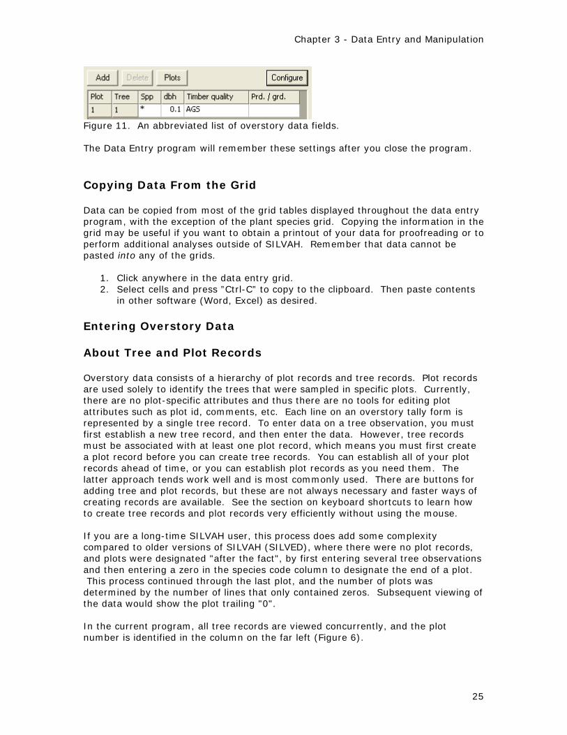
Figure 11. An abbreviated list of overstory data fields. The Data Entry program will remember these settings after you close the program.
Copying Data From the Grid
Data can be copied from most of the grid tables displayed throughout the data entry program, with the exception of the plant species grid. Copying the information in the grid may be useful if you want to obtain a printout of your data for proofreading or to perform additional analyses outside of SILVAH. Remember that data cannot be pasted into any of the grids.
1. Click anywhere in the data entry grid. 2. Select cells and press ”Ctrl-C” to copy to the clipboard. Then paste contents
in other software (Word, Excel) as desired.
Entering Overstory Data
About Tree and Plot Records
Overstory data consists of a hierarchy of plot records and tree records. Plot records are used solely to identify the trees that were sampled in specific plots. Currently, there are no plot-specific attributes and thus there are no tools for editing plot attributes such as plot id, comments, etc. Each line on an overstory tally form is represented by a single tree record. To enter data on a tree observation, you must first establish a new tree record, and then enter the data. However, tree records must be associated with at least one plot record, which means you must first create a plot record before you can create tree records. You can establish all of your plot records ahead of time, or you can establish plot records as you need them. The latter approach tends work well and is most commonly used. There are buttons for adding tree and plot records, but these are not always necessary and faster ways of creating records are available. See the section on keyboard shortcuts to learn how to create tree records and plot records very efficiently without using the mouse. If you are a long-time SILVAH user, this process does add some complexity compared to older versions of SILVAH (SILVED), where there were no plot records, and plots were designated "after the fact", by first entering several tree observations and then entering a zero in the species code column to designate the end of a plot. This process continued through the last plot, and the number of plots was determined by the number of lines that only contained zeros. Subsequent viewing of the data would show the plot trailing "0". In the current program, all tree records are viewed concurrently, and the plot number is identified in the column on the far left (Figure 6).
25

SILVAH Users Guide
Figure 6. An example set of tree records showing plot numbers in the far left column.
How to Get Started
It is easy to get started adding tree data, and if you prefer to add plots as you go -- that is, handling the creation of plot records with a only slight amount of extra effort, you can begin by following the steps below:
1. Start the Data Entry program, and click "Enter Inventory Data" in the Navigation Pane. Then click "Trees" in the Options Pane.
2. In the Work Pane, either click the "Add" button once, or mouse over into the large gray area and click anywhere (Figure 7). This step will automatically create the first plot record and also establish the first tree record for you.
3. Proceed with entering data for the first observation, as shown in Figure 8. Default values for new tree records
26

Chapter 3 - Data Entry and Manipulation
There are a limited number of fixed default values that appear every time you create a tree record (Figure 8). Timber quality is Acceptable Growing Stock (AGS) and diameter at breast height (d.b.h.) is 0.1 inches. The number of trees represented by this observation (the count) is 1, and defect is assumed to be zero.
Figure 7. Getting started with overstory data entry.
Figure 8. The first tree record.
27

SILVAH Users Guide
Entering the Data
The species code, diameter, and quality fields should be completed for each observation, and the remaining fields are optional, and may be left blank if desired. Entering Species Codes When you begin entering data for a new tree, type in the species code of the first observation (tree) and hit either the enter key or the right arrow key. The species entries are NOT case sensitive and will be displayed in upper case. If you type in a species code that does not exist, you will be presented with a pop-up list to choose from. The list is initially sorted by the species code specified under Inventory Settings. Select a species from the list and click "OK". If you select Cancel, the species cell is returned to the previous value. To learn more about how to identify a species during data entry -- see "about species codes" in Chapter 4 on setting up defaults. Entering the Diameter When the species code is accepted the program will move to the next field to the right, which is the "diameter" field. Enter the diameter of the observed tree. SILVAH works only with whole numbers, and if you enter more precise values, the display will retain them, but only rounded values will be stored in the data (.SIL) file. If applicable, you may only need to record even numbers if your cruise is by 2-inch size classes. If you are using broad size classes, then use only the midpoints of the diameter classes. You will not be able to enter numbers larger than the maximum 40 inches. Entering the Quality The "quality" field is the next one to be filled in. You may record AGS, UGS, or dead. If you are using a prism cruise, you may also record borderline AGS, borderline UGS, or borderline dead. Type in a legal code and hit the enter or right arrow key to move to the next field. The species code, diameter, and quality fields must be completed for each observation. Entering Merchantable Height or A Tree Count The inventory and grading information under Inventory Settings determines which value is entered in the next field. Specifically, if you indicate that your tree observations contain counts ,then the data entry program will display a count field. If you indicate that your tree observations contain heights, then you will see a field for merchantable height. There are actually two separate variables, one for counts, and another for merchantable heights, but the program will not allow both to be used at the same time -- only one of them will be available. Entering Grade, Defect, Crown, Wildlife Codes The remaining four fields, for grade, defect, crown condition, and wildlife code are completed in a similar way. All four of these fields are optional, and need not be filled in. The grade, crown, and wildlife are all coded values. The codes and meanings can be found in Table X in the Appendix. Defect is also described there, and is a percentage recorded as tens of percent; that is, 1 for 10 percent, 2 for 20 percent, and so on.
28

Chapter 3 - Data Entry and Manipulation
Proceeding to the next tree observation When you reach the end of a row, if you press the enter key after editing the last field, and this is last observation in the current plot, a new tree will be added automatically, otherwise, you will jump to the next row below. Repeat this procedure and enter one observation for each line on your tally form. When you are ready to add a new observation that begins in the next plot, instead of pressing the enter key, press [Ctrl][Shift][Enter] - that is, press and hold down the control key and the shift key at the same time and then press the enter key. Refer to the section on Working with Grid Tables for data entry shortcuts (in this chapter) for more information. You should periodically save your work while you are entering data to avoid losing information and having to start over.
Adding Tree Observations
Tree observations can be added or inserted at any time. It is most efficient to add trees as you need them during initial data entry, such as when you are finished with one record and then press the enter key to start another tree record in the current plot. See the section on entering the data, and be sure to review the data entry shortcuts in the section on Working With Grid Tables in this chapter. These instructions mainly apply to situations such as when you discover that you inadvertently skipped a tree the first time around. Adding a Tree Record
1. Start the Data Entry program, and click "Enter Inventory Data" in the Navigation Pane. Then click "Trees" in the Options Pane.
2. In the Work Pane, click the "Add" button. 3. Select an existing plot to add the tree record as the last tree in the plot, OR
click "Add a New Plot" if you want to establish the new tree record as the first record in a new plot.
4. Click "OK" if necessary. Inserting a Tree Record
1. Start the Data Entry program, and click "Enter Inventory Data" in the Navigation Pane. Then click "Trees" in the Options Pane.
2. Click anywhere in the row of an existing tree record. 3. Press [Ctrl] [Enter] to insert a new tree record below the existing one.
Manipulating Plots
If the need arises, you can rearrange plots even after you have entered data. This would result in a renumbering of all plots according to the order you want. You can also insert a plot at any time, and this may be important if order is critical and you discover later that you inadvertently skipped a plot or entered data out of order. Change Plot Order
29

SILVAH Users Guide
1. Start the Data Entry program, and click "Enter Inventory Data" in the
Navigation Pane. Then click "Trees" in the Options Pane. 2. Click "Plots" at the top of the Work Pane to launch the dialog as shown in
Figure 12. 3. In the list of existing plots, drag-and-drop the plot to its appropriate place on
the list. 4. Click "OK" when you are finished.
Figure 12. Manipulating overstory plots. Add a Plot
1. Start the Data Entry program, and click "Enter Inventory Data" in the Navigation Pane. Then click "Trees" in the Options Pane.
2. Click "Plots" at the top of the Work Pane to launch the dialog as shown in Figure 12.
3. Click the "Add" button, and you will see "New Plot 1" appear at the bottom of the list.
4. Drag-and-drop the plot to its appropriate place in the list if you don't want it to be the last plot in the group.
5. Click "OK". Insert a Plot
1. Start the Data Entry program, and click "Enter Inventory Data" in the Navigation Pane. Then click "Trees" in the Options Pane.
2. Click "Plots" at the top of the Work Pane to launch the dialog as shown in Figure 12.
3. Click on one of the existing plots where you wish to insert a plot. 4. Then click the "Insert" button. 5. Choose whether to insert the plot before or after the highlighted plot. 6. Click "OK".
Delete a Plot
1. Start the Data Entry program, and click "Enter Inventory Data" in the Navigation Pane. Then click "Trees" in the Options Pane.
30

Chapter 3 - Data Entry and Manipulation
2. Click "Plots" at the top of the Work Pane to launch the dialog as shown in Figure 12.
3. In the list of existing plots, click on the one you wish to delete. Note: all tree observations in the plot will also be deleted.
4. Click the "Delete" button. 5. Click "OK". If you accidentally deleted the wrong plot, click "Cancel" and try
again.
Entering Understory Data
About Understory Data
Understory observations are recorded by plot, and there are no records below the plot level. There are two ways that understory data can be collected, and what you see will depend on the understory cruise type you specified under Inventory Settings. The first, and most common, is what is known as "Extended" regeneration data, where you enter weighted counts of seedlings, percent cover, and understory data codes directly from the regeneration tally. You will be entering data for each plot separately -- each column represents a plot. The other, less common and older method is known as the "Checkmark" tally. With this method, you enter the number of plots stocked with each category of regeneration or interfering plants. If you select the Checkmark method under Inventory Settings, you must also enter the number of checkmark plots tallied in the field before completing the Inventory Settings. The presence of non-native invasive species may be noted while sampling. For further information, see the section on Non-Native Species Data.
Entering extended regeneration data
This is the preferred and most beneficial of the methods for collecting understory data because you are collecting and retaining quantitative data that can be analyzed against known criteria in an objective manner, and it allows for a more meaningful comparison with data in the future. You can begin an extended regeneration tally by following the steps below:
1. Start the Data Entry program, and click "Enter Inventory Data" in the Navigation Pane. Then click "Understory plots" in the Options Pane.
2. In the Work Pane, either click the "Add" button once, or mouse over into the large gray area and click anywhere (Figure 13). This step will automatically create the first understory plot record.
3. Proceed with entering data for the first understory plot, as shown in Figure 14.
4. Click the Add button any time you need to add another understory plot.
31

SILVAH Users Guide
Figure 13. Getting started with extended understory data.
Figure 14. The first understory plot The desirable regeneration data is represented in the upper half of the rows in the understory data grid. Lower rows contain interfering vegetation and site limitations. After you enter a value, when you press the enter key you will move down to the next row in the plot. Desirable Regeneration
32

Chapter 3 - Data Entry and Manipulation
Enter the weighted counts of black cherry, tulip poplar, new oak, established oak, competitive oak, other desirable species, and conifers. Items With Species Enter the appropriate species code when applicable. Species are identified and stored as explained in the section on tree data, entering species codes. Also see "about species codes" in Chapter 4 on setting up defaults for more information on how to identify species during data entry. Percent Cover For these items, enter the percent cover using whole numbers such as 15%, 70%, and so on. Total Height of Oak Seedlings This applies to the Pennsylvania State University Appalachian Oak Guide. It represents, to the nearest 1/2 foot, the total combined height of all oak seedlings in the regeneration plot. Grape Vines This is the total count of grapevines that have ascended into the overstory. Thick Duff, Rocky Surface, Poor Drainage Answer yes/no for these items if they characterize the interference plot. Proceeding to the next understory plot When you reach the end of a column (plot), press [Ctrl] [Enter] to start another understory plot, or click "Add" at the top of the Work Pane. Refer to the section on Working With Grid Tables for data entry shortcuts (in this chapter) for more information. Deleting an understory plot To delete an existing plot, click anywhere inside the column of the plot you wish to delete, and then click on the "Delete" button at the top of the Work Pane. You should periodically save your work while you are entering data to avoid losing information and having to start over.
Entering checkmark regeneration data
Checkmark data is quick but rather subjective, and is based on field judgement at the time of sampling. You can begin a checkmark tally by following the steps below:
1. Start the Data Entry program, and click "Enter Inventory Data" in the Navigation Pane. Then click "Understory plots" in the Options Pane.
33

SILVAH Users Guide
2. Proceed with entering data for the first understory plot, as shown in Figure 15.
3. If you do not see the arrangement of fields as in Figure 15, it may be that you need to specify the Checkmark tally under Inventory Settings.
Figure 15. Getting started with checkmark understory data. Enter the number of plots stocked with each category of regeneration or interfering plants. The maximum value for any field is the same as the number of regeneration plots taken. You will not be able to enter any number greater than that. If necessary, you can change the number of regeneration plots at the top of the form. This is the same value that is entered under Inventory Settings. There are a several rules that apply. The "established" and "competitive" desirables sub-total fields must be at least as much as any of the individual regeneration fields. The "total oak" field must be at least as much as any of the individual oak regeneration fields, and the "established oak" regeneration field must be less than or equal to the "established" desirables sub-total field. The "any interference" field must be at least as much as any of the individual interference fields. These validations are done when you try to move elsewhere within the program. If there are errors, you will get an appropriate message. When you are finished, be sure to save your work to avoid losing information and having to start over.
Entering Non-Native Invasive Species
About Non-Native Invasive Species Data
Non-native invasive species (NNIS) may be present in or adjacent to the stand. Without being aware of their presence, any disturbance that reduces competition, increases light, or disturbs the soil may result in a rapid and near-complete dominance of the ground cover and the understory by aggressive non-native species,
34
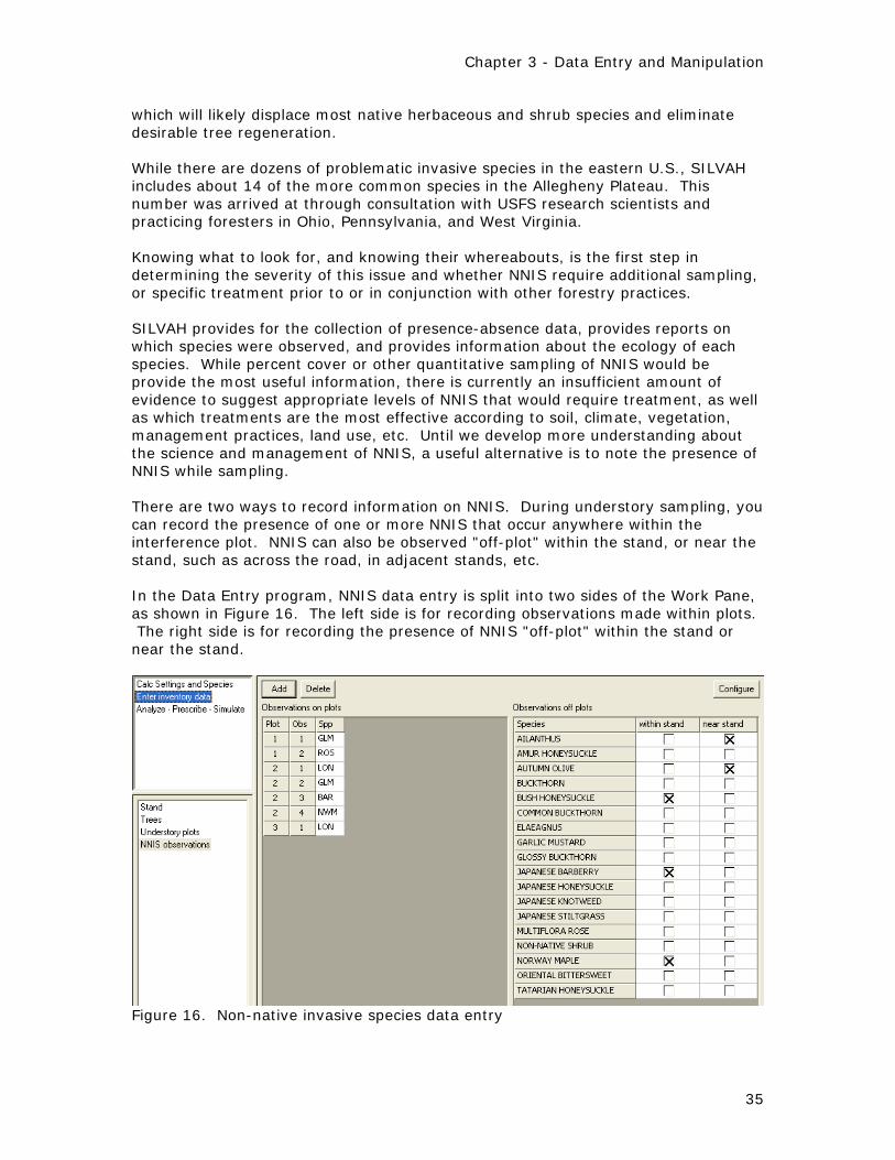
Chapter 3 - Data Entry and Manipulation
which will likely displace most native herbaceous and shrub species and eliminate desirable tree regeneration. While there are dozens of problematic invasive species in the eastern U.S., SILVAH includes about 14 of the more common species in the Allegheny Plateau. This number was arrived at through consultation with USFS research scientists and practicing foresters in Ohio, Pennsylvania, and West Virginia. Knowing what to look for, and knowing their whereabouts, is the first step in determining the severity of this issue and whether NNIS require additional sampling, or specific treatment prior to or in conjunction with other forestry practices. SILVAH provides for the collection of presence-absence data, provides reports on which species were observed, and provides information about the ecology of each species. While percent cover or other quantitative sampling of NNIS would be provide the most useful information, there is currently an insufficient amount of evidence to suggest appropriate levels of NNIS that would require treatment, as well as which treatments are the most effective according to soil, climate, vegetation, management practices, land use, etc. Until we develop more understanding about the science and management of NNIS, a useful alternative is to note the presence of NNIS while sampling. There are two ways to record information on NNIS. During understory sampling, you can record the presence of one or more NNIS that occur anywhere within the interference plot. NNIS can also be observed "off-plot" within the stand, or near the stand, such as across the road, in adjacent stands, etc. In the Data Entry program, NNIS data entry is split into two sides of the Work Pane, as shown in Figure 16. The left side is for recording observations made within plots. The right side is for recording the presence of NNIS "off-plot" within the stand or near the stand.
Figure 16. Non-native invasive species data entry
35

SILVAH Users Guide
Entering Plot-based NNIS Observations
NNIS observations observed within interference plots are entered in a manner similar to tree data, using understory plots as the basis. If you have already entered understory data, then you do not need to establish understory plots again -- you will use the same plots for recording NNIS observations. To enter data on an NNIS observation, you must first establish a new NNIS observation record, and then enter the data. NNIS records must be associated with at least one plot record. You will need to choose from the list of existing understory plots (or create new plots if necessary) before you can create NNIS records. Getting Started After Entering Understory Data
1. Start the Data Entry program, and click "Enter Inventory Data" in the Navigation Pane. Then click "NNIS observations" in the Options Pane.
2. In the Work Pane, click the "Add" button once. 3. From the pop-up "choose a plot" dialog, click on the plot that contains the
NNIS observation you wish to create. Note: if you double-click on a given plot, you can skip step 4.
4. Click OK. Getting Started Without Existing Understory Data (No Plot Created Yet)
1. Start the Data Entry program, and click "Enter Inventory Data" in the Navigation Pane. Then click "NNIS observations" in the Options Pane.
2. In the Work Pane, click the "Add" button once. This step will automatically create the first understory plot record and also establish the first NNIS observation record for you.
Entering the data Currently, only the identification of species is required. No other data can be recorded. Please see the instructions on entering species codes in the section on entering overstory data for further information on how to record species. Be aware that FIA codes may not have existed for many of the non-native species, as early FIA data was targeted mainly at trees and other frequently observed woody shrubs. The FIA codes displayed for NNIS may be arbitrary but can be used throughout the program to recognize the species. If you enter a native species that is "invasive", or any species that is NOT marked as exotic under Plant Species information, the species cell will be hilited in yellow (Figure 17) to distinguish native species from non-native ones.
36

Chapter 3 - Data Entry and Manipulation
Figure 17. Distinguishing native species (yellow) from other NNIS entries. Adding new understory plots If you need to add additional understory plots, you may create them during understory data entry, or while entering NNIS observations.
1. Start the Data Entry program, and click "Enter Inventory Data" in the Navigation Pane. Then click "NNIS observations" in the Options Pane.
2. In the Work Pane, click the "Add" button once. 3. From the pop-up "choose a plot" dialog, click on the "Add new plot" button.
Deleting understory plots If you need to delete an understory plot, it must be done through understory data entry. Please see the instructions for deleting an understory plot in the section on entering extended regeneration data. Proceeding to the next NNIS observation When you reach the end of a row, if you press the enter key after editing the last field, and this is last observation in the current plot, a new NNIS observation will be added automatically, otherwise, you will jump to the next row below. When you are ready to add a new observation that begins in the next plot, instead of pressing the enter key, press [Ctrl][Shift][Enter] - that is, press and hold down the control key and the shift key at the same time and then press the enter key. Refer to the section on Working With Grid Tables for data entry shortcuts (in this chapter) for other important shortcuts.
Entering Off-plot NNIS Observations
Off-plot NNIS observations are recorded on a list of known exotic invasives in your sampling area. Before you can record your off-plot observations, you must first establish a list of exotic species. This list is used for species observed within the stand and near the stand, and is displayed on the right-hand side of the Work Pane (refer to Figure 16 in the introduction on Non-native Invasive Species Data). Your observations are made by checking off species from the list.
37

SILVAH Users Guide
38
Establishing a list of exotic species
1. Start the Data Entry program, and click "Calc Settings and Species" in the Navigation Pane. Then click "Plant species information" in the Options Pane.
2. Make sure the "Exotic" column is in display. If it is not, try scrolling, or click the "Configure" button to rearrange the plant species fields in the grid. See the instructions for configuring data fields in the grid for further information.
3. In the species row, enter "yes" (or the letter "y") in the exotic field. Repeat this process for all species that should be considered exotic in your area.
To see all of the exotic species together, try sorting by the exotic field. Click once in the header of the exotic column to sort in ascending order, and click again to sort in the opposite order. Entering the data When you are ready to record your off-plot NNIS observations, follow these steps:
1. Start the Data Entry program, and click "Enter Inventory Data" in the Navigation Pane. Then click "NNIS observations" in the Options Pane.
2. If you do not see any species to the far right-hand side, that probably means there are currently no species marked as exotic under Plant Species. Refer to the instructions above on establishing a list of exotic species.
3. For off-plot observations made within the stand, check the appropriate species under the "within stand" column on the right-hand side of the Work Pane.
4. For off-plot observations made outside the stand, check the appropriate species under the "near stand" column on the right-hand side of the Work Pane.

Chapter 4 - Setting Up a Defaults File
About SILVAH defaults
The defaults file(s) (.DEF) contains information on local stumpage prices, the log rule you want to use, a list of your own species codes (if you do not like ours), which directory you will use for data, where you want your reports sent, and so on. This feature of SILVAH makes the program very convenient. Every time you load the Analysis and Prescription or TREECALC programs, you will be asked the name of the defaults file you want to use; then that defaults file will be read. There are default values for all parameters in the program, so you do not absolutely have to have a defaults file. If you do not have one, you will be warned each time you run the Analysis and Prescription program that it is using the default values we have coded into the program. But the default values in the program are ones that we find convenient for our computers and our forest conditions in northwestern Pennsylvania. You can change those values to suit your situation, and the SILVAH programs will use your values every time they are run. So, you should create a defaults file in the Data Entry program. A sample defaults file (SILVAH.DEF) is installed with the program into the default data directory. You may want to open this file to examine the defaults, and if desired, modify the defaults as necessary. Some users will find it convenient to create more than one defaults file, especially if you work in several different geographic areas where stumpage prices vary, for example. Thus, you could create a defaults file for each area, and then read the appropriate one when running the Analysis and Prescription program or TREECALC.
Starting a New Defaults File
To start a new defaults file, follow these steps:
1. Start the Data Entry program. 2. Click "Calc Settings and Species" in the Navigation Pane. 3. From the top menu, click "File", then click "New DEF File". 4. Review and modify the calculation settings, system settings, and plant species
information as appropriate. These items can be selected in the Options Pane. 6. Be sure to save your work. Your defaults will be stored in a new defaults
(.DEF) file. You may also try the shortcut, "[Ctrl] + [N]" (press and hold the control key and then press the letter "N"), to start a new file.
Opening An Existing Defaults File
To open an existing file:
39
SILVAH Users Guide
1. Start the Data Entry program. 2. If not already selected, click "Calc Settings and Species" in the Navigation
Pane. 3. From the top menu, click "File", then click "Open DEF File".
You may also try the shortcut, "[Ctrl] + [O]" (press and hold the control key and then press the letter "O"), to open a defaults file.
Saving Your Defaults
To save the current defaults to a file:
1. If not already selected, click "Calc Settings and Species" in the Navigation Pane.
2. From the top menu, click "File", then click "Save DEF File". 3. Enter a file name, and be sure you are aware of the folder where the file is
being created. It is recommended that you store the file in the default data directory if you intend on using this defaults file frequently.
You may also try the shortcut, "[Ctrl] + [S]" (press and hold the control key and then press the letter "S"), to save the file.
Converting Older Defaults Files
SILVAH has been around for some time. As it evolved, additional capabilities have been added. Along with those additions came format changes in the defaults files. The data entry program has the capability to convert defaults from older formats -- at least back to version 4.0 -- and convert them to the current version format. The program attempts to read the old formats directly, and when you save the file, the defaults will be saved in the new format. Converting older defaults requires a few simple steps, as well as reviewing the data to ensure it was correctly interpreted:
1. If not already selected, click "Calc Settings and Species" in the Navigation Pane.
2. Open the defaults (.DEF) file with the older format. 3. Once the defaults have been loaded, review the data to be sure it is accurate.
Pay close attention to plant species information. 4. Save the file (perform a "Save - As"). It is recommended that you use a
slightly different file name in order to preserve the contents of the original defaults file.
Calculation Settings
Default Management Values
These values allow you to supply management-oriented values that generally do not change very often. This is simply a matter of convenience , saving you the effort of reentering these values for each stand, since they usually remain the same for a particular user.
40

Chapter 4 - Setting Up a Defaults File
Management values have always been stored in your data (.SIL), and they are no longer stored as part of the defaults (.DEF) file. However, you can still specify default values, and the Data Entry program will remember them for you. Each time you open the Data Entry program, if you have elected to store management values as defaults, they will be loaded automatically by the program. To establish default management values, refer to the instructions on management information under Chapter 3 on data entry and manipulation for further information. The following are management-oriented values: Owner Management Value Restrictions on Silvicultural System Prescription Charts To Follow Intend to Regenerate Increase oak Residuals Desired Operability Accessibility Deer impact
Default Inventory Settings
Inventory settings are not likely to change very often. Therefore, you can specify a set of default values that you can use over and over again. This is simply a matter of convenience , saving you the effort of reentering these values for each stand, since they usually remain the same for a particular user. Inventory settings have always been stored in your data (.SIL), and they are no longer stored as part of the defaults (.DEF) file. However, you can still specify default values, and the Data Entry program will remember them for you. Each time you open the Data Entry program, if you have elected to store inventory settings as defaults, they will be loaded automatically by the program. To establish default inventory settings, refer to the instructions on inventory settings under Chapter 3 on data entry and manipulation for further information. The following are inventory-related values: Overstory cruise type BAF or fixed overstory plot size Observations include counts or merchantable heights Tree Grading Procedure Understory cruise type Understory plot size Species code type used in data DBH size classes used in data Tally month and year
41

SILVAH Users Guide
Default Commercial Sale Breakpoints
The top set of values in Figure 18, under the subheading "Commercial Sale Breakpoints" specifies how much volume must be available for SILVAH to prescribe a commercial cutting. For example, the defaults shown below require a minimum of 2,000 board feet to be removed during a sawtimber only sale. If there is insufficient volume available for such a sale, SILVAH will check to see if there is 1,500 board feet and 5 cords to make an integrated sale. If there is not enough volume for an integrated sale, SILVAH will check to see if 7 cords are available for cutting in a pulpwood only sale. If the volume is inadequate to support any of these commercial sale minimums, SILVAH will prescribe no cutting. Setting default commercial sale breakpoints
1. Start the Data Entry program, and click "Calc Settings and Species" in the Navigation Pane. Then click "Calculation parameters" in the Options Pane.
2. In the Work Pane, enter the values under "Commercial Sale Breakpoints" as appropriate.
3. Remember to save your work. Doing so will place your values into a defaults (.DEF) file that you can use with the Analysis and Prescription program.
42

Chapter 4 - Setting Up a Defaults File
Figure 18. Setting timber sale breakpoints in the data entry program.
Default Diameters for Volumes
The second set of values in Figure 18, under the subheading "Minimum Diameter for Volume Estimates" is the threshold diameters for calculating volumes. For example, hardwood sawtimber volumes will be calculated for trees larger than 10.5 inches (11-inch class if you use 1-inch classes, or 12-inch class if you use 2-inch classes) as shown in Figure 18. You can set any threshold diameter you wish for these calculations. Setting the threshold diameter to 41 inches will prevent any calculation of volumes. Thus, you could prevent pulpwood volume from being calculated (if you have no pulpwood market, for example) by setting minimum diameter for pulpwood to 41 inches. Setting default threshold diameters for calculating volumes
1. Start the Data Entry program, and click "Calc Settings and Species" in the Navigation Pane. Then click "Calculation parameters" in the Options Pane.
2. In the Work Pane, enter the values under "Minimum Diameter for Volume Estimates" as appropriate.
43

SILVAH Users Guide
3. Remember to save your work. Doing so will place your values into a defaults (.DEF) file that you can use with the Analysis and Prescription program.
Default Log Rule and Other Values
The following are several additional default settings that affect calculations by the Analysis and Prescription and TREECALC programs. Setting default calculation values
1. Start the Data Entry program, and click "Calc Settings and Species" in the Navigation Pane. Then click "Calculation parameters" in the Options Pane.
2. In the Work Pane, enter the values under the subheading "Other" as appropriate (Figure 18).
3. Remember to save your work. Doing so will place your values into a defaults (.DEF) file that you can use with the Analysis and Prescription and TREECALC program.
Log Rule You can specify a default board foot log rule, as well as several other values. The log rules are International 1/4", Doyle, and Scribner. Trees Included Specify whether to include live trees only, live and dead, or only dead trees in your calculations. Name of local log and boltwood product You can specify the names you want to use (and that will be used on your reports) for one bulk and one log product. For example, if you have a pallet log market or a railroad tie market, you can define that product name here. Sugar maple site condition Sugar maple growth and seed production are affected by site quality. The seed source calculation of the Analysis and Prescription program utilizes this value. Use NY relative density equation If you are in southern New York, you can use a relative density equation that accounts for site differences. Species codes (TREECALC) Specify the species codes you prefer to use when running the TREECALC program. This setting is not used elsewhere.
System Settings
Default Output Folders
You can specify default locations on your computer for data, reports, and script/batch files. Specifying default folders will help you avoid typing that folder each time you specify a file. When you are asked for a file name, you need only type the file name, not the entire folder location (pathname). However, if you have a file
44

Chapter 4 - Setting Up a Defaults File
in another folder you can always type the full drive/path/file name and program will use that rather than the default. See the section, "Managing your files", for additional information on the data, output, and script/batch folders. To specify default folder locations:
1. Start the Data Entry program, and click "Calc Settings and Species" in the Navigation Pane. Then click "System settings" in the Options Pane.
2. In the Work Pane, click the BROWSE button next to each folder entry (Figure 19) to specify a default folder that you want the Analysis and Prescription program to use.
The program will NOT accept manual text entry, in order to prevent inadvertent creation of new folders. Just use the browse button. If you need to create a new folder on your computer, use Windows Explorer to do that first, and then browse to the new folder.
Figure 19. Establishing default output folders in the data entry program.
Default Operation Mode
You can specify how you want the Analysis and Prescription program to operate each time it is run, such as Interactive, Script, or Batch mode. See Chapter 1 for further information about the different "Operation Modes". Setting the Default Operation Mode
1. Start the Data Entry program, and click "Calc Settings and Species" in the Navigation Pane. Then click "System settings" in the Options Pane.
2. In the Work Pane, make a selection from the pick list for how you want SILVAH to interact (Figure 19).
Plant Species Information
45

SILVAH Users Guide
About Species Codes
The program will only use one of 3 possible codes, either the FIA, Mnemonic, or User code, to display your species entries and to store species in your data. However, there are additional ways to identify a species, according to any of several possible species identifiers shown below. This may be advantageous if you remember one identifier but not the one that belongs to the set of codes you have specified under Inventory Settings. For example, if have chosen the Mnemonic species code under Inventory Settings, and you enter "318" -- the FIA code for sugar maple, the program will recognize the species and display "SM" in the species field because "SM" is the mnemonic code. If you could not remember either of these codes, you could try entering the common name, such as "sugar maple", and the program would display "SM". The code "SM" is stored in the data (.SIL) file.
• FIA - The original US Forest Service Forest Inventory and Analysis Codes. A 3-digit numeric code that was formerly used throughout the United States. Acceptable in SILVAH.
• USDA Plants Symbol - This is a new identifier that replaced the FIA codes, it is
the first two letters of the genus and the first two letters of the species, followed by a number if there are other plants that have similar genus and species abbreviations. This code is not editable by the user, as it is maintained in the PLANTS database developed by the USDA Natural Resources Conservation Service for every species found in North America (native or exotic). The data entry program will readily interpret these codes, but they will never show up in the display, nor will they appear in the data (.SIL) file.
• Mnemonic - A user-defined code, typically 2 or 3 letters that abbreviate the
common name. Used on all reports, regardless of what code occurs in the data. Based on the first letter of the common name to represent individual species (thus, SM for sugar maple), and the first letters of the common genus name to represent an entire genus (thus, B for birch). You can change these abbreviations to meet your own needs, if desired.
• User Defined (Local) - Another user-defined code, allowing only numeric
values. Often used to represent multiple species of a genus or family, such as "pine", "conifers", and so on.
• Common name - The common name of the species. The data entry program
will readily interpret the common name, but it will never show up in the display, nor will it appear in the data (.SIL) file.
Number of species Currently there are 130 species included in the program, mostly trees, some woody shrubs, and a few non-native invasive herbaceous species. This is a fixed list of species, representing those most likely to be encountered in the Allegheny Plateau of Pennsylvania, New York, Ohio, Pennsylvania, and Maryland. You may not change the species that are included.
46

Chapter 4 - Setting Up a Defaults File
Sorting the display of species You can sort the display of species by any of the species attributes. This is very useful in searching for species as well as examining prices or other attributes. To sort by an attribute, click once in the header of the column that contains the attribute. The first click will toggle the sort in descending order, and second click will sort in ascending order. Configuring the display of species attributes in the grid If you prefer, you can rearrange the order of the columns of species attributes, or turn on/off attributes that you do not intend to use. See the instructions for configuring data fields on the grid, in the section on working with grid tables.
Default Species Codes
You can edit the mnemonic or the user species codes. Other identification codes displayed in the gray columns are not editable. If you are about to edit species codes that have previously been used in data (.SIL) files, please see the warning below to learn how to avoid possible loss of data. Setting species codes
1. Start the Data Entry program, and click "Calc Settings and Species" in the Navigation Pane. Then click "Plant species information" in the Options Pane.
2. In the Work Pane, move to the field you want to change and type in the new value that you want to use (see Figure 20).
Warning! If you decide to alter the local or mnemonic species codes, and you have already collected data using the default codes (or other versions of your own codes), be careful! When you run the old data files through SILVAH, you will need to load and use the old defaults file so that species codes are interpreted properly. Therefore, you should save a copy of the old defaults file before you alter the species codes. A better solution is to convert the species codes in your old data files to the new codes. That way, you will need to maintain only one defaults file for species codes. SILVED will make the conversions automatically for you, but you must do this in the proper sequence to avoid loss of data. Proceed as follows.
1. Make backup copies of all data files to be converted to the new codes, in case something goes wrong.
2. Make certain that you have copies of both your old defaults file (containing the old species codes), and your new defaults file containing new species codes. Obviously, these two files must have different names.
47

SILVAH Users Guide
If you edited the original defaults file and saved the revision under the same name, you'll need to recreate the old defaults file. You can recreate the defaults file included with the program by simply starting a new defaults file and then saving the built-in defaults.
3. Start the data entry program, click "Calc Settings and Species" in the
Navigation Pane, and click "File - Open" to load the original defaults file containing the old species codes.
4. Click "Enter Inventory Data", then click "File - Open" Retrieve the data file containing the old codes.
5. Return to "Calc Settings and Species", then click "File - Open" to load the new defaults file that contains your new codes.
6. Then return to "Enter Inventory Data", and review the code in the inventory data. The old codes should now be replaced by the new codes.
7. Click "File - Save As" to save a new copy of the data file. Be sure not to overwrite the original version that had the original species codes.
Figure 20. Setting plant species defaults. Species are shown sorted in ascending order by mnemonic code.
Default Species Parameters
48

Chapter 4 - Setting Up a Defaults File
49
In addition to species identification codes, there are other parameters associated with each species, including form class, volume correction factors, and stumpage prices for various products. You should edit these values to reflect conditions in your area. Setting default species parameters
1. Start the Data Entry program, and click "Calc Settings and Species" in the Navigation Pane. Then click "Plant species information" in the Options Pane.
2. In the Work Pane, move to the field you want to change and type in the new value that you want to use (see Figure 20). When you are finished editing these values, be sure to save your defaults (.DEF) file.
Form This column is the form class that will be used in calculating volumes. Girard-Mesavage form class volume tables are used. Pulp VC, Saw VC These are columns that may be used to adjust the volumes, both sawtimber and pulp. If you find that the program consistently gives high or low volumes for a species, then you may change these factors to more reasonably reflect your volumes. Exotic This column denotes whether a species is not native to your area. If you wish to obtain reports on non-native species in your data, you must identify exotic species as appropriate. Desirable This column denotes whether a species is desirable, for any reason. During data entry, if you try to record a sapling of undesirable species, you will be warned that the regeneration plot will NOT be considered stocked with saplings since you recorded an undesirable species. Prices There are several columns that provide the stumpage values for sawtimber, veneer, pulp, local bulk, and local sawlog products.

Chapter 5 - Analysis and Prescription
Starting Analysis and Prescription
To start the Analysis and Prescription Program, click "Start - Programs - SILVAH - Analysis and Prescription". You can also run the program from the Data Entry Program, by clicking "Analyze - Prescribe - Simulate" in the Navigation Pane. The Analysis and Prescription program will begin with the following question: "Name of defaults file:" Either accept the defaults file name on the screen (SILVAH.DEF) by hitting [Enter], or type in the name of the defaults file you want to use; then hit [Enter]. The program will respond with one of the two following messages:
• "Retrieving default values from disk ..."
This means that you have created a set of customized default values and stored them in a disk file (usually called SILVAH.DEF). These default values tell the program which log rule, form classes, stumpage prices, and so on, to use. The program will ask for this file each time you load the program.
• "Your customized defaults file was not found. Therefore, the defaults currently in memory will be used. The standard defaults are listed in the documentation. To create and save a customized defaults file, use the Calc Settings and Species module of the Data Entry Program. Hit any key to continue."
This either means that you have never created a customized defaults file, or that SILVAH cannot find it. When you hit the next key, SILVAH will go ahead and run using the defaults coded into the program.
If you have not created a customized defaults file, you should do so before you run any real data. Follow the instructions in Chapter 4 on setting up a defaults file. If you have created a defaults file and the Analysis and Prescription program cannot find it, examine the folders on your computer to locate it. Also, check to see that the defaults file has the correct name; usually it is called SILVAH.DEF, unless you told SILVAH to use a different name. See Chapter 4 for further information. Main menu After the defaults file is loaded, or after you hit any key following the message that the program cannot find your defaults file, the main menu will appear (Figure 21).
50

Chapter 5 - Analysis and Prescription
Figure 21. Main menu of the Analysis and Prescription program
Notice that you have six options at this point, each described briefly in the menu. The program is expecting you to choose one of those options and type a number from 1 to 6 indicating your choice. Notice also that the blinking cursor is positioned in the proper spot to accept your response, and that SILVAH has taken a guess as to what your response will be. The program has guessed that you will choose option 4 to run the program. You will find that the Analysis and Prescription program almost always takes a guess at which option you will choose in the various menus. This will save you time once you get used to it, because all you need do is press the enter key if you agree with the initial choice. However, if you want to try a different option, just type the number of your choice (it will replace the default) and hit the enter key.
Changing Runtime Options
The values that initially appear as runtime options when you start the Analysis and Prescription program are determined by your defaults (.DEF) file. You can change the operation mode and the trees to include in your defaults file so that you need not change them each time you start the Analysis and Prescription program. However, occasionally you might need to change the runtime options, or, if you want to learn what they are, select option 3 from the main menu. This will bring up the runtime options menu (Figure 22). Note that there are two groups of options, and that the currently selected option in each group is indicated by an asterisk. You can make only one selection from each of the two groups, and you must make a selection in each group. The program has guessed that you will return to the main menu without making any changes, and if this is your choice, press the enter key. If you wish to change any of the options, type the option number desired and press the enter key. Once you have selected the options you want, select option 7 and press the enter key to return to the main menu.
51
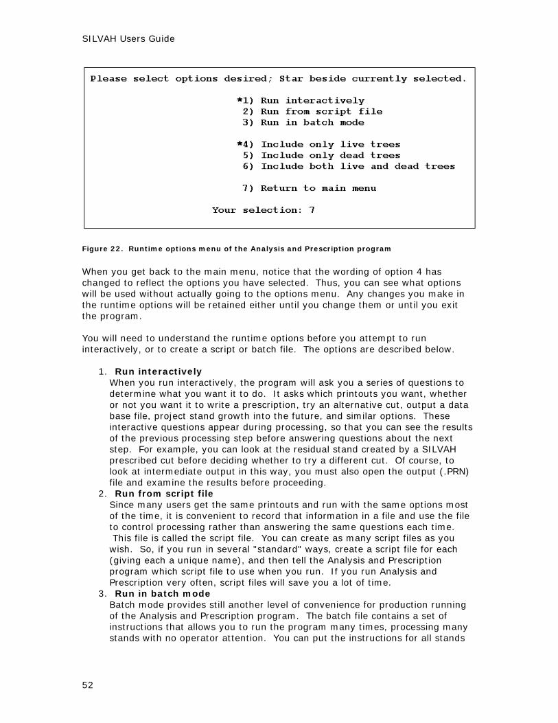
SILVAH Users Guide
Figure 22. Runtime options menu of the Analysis and Prescription program
When you get back to the main menu, notice that the wording of option 4 has changed to reflect the options you have selected. Thus, you can see what options will be used without actually going to the options menu. Any changes you make in the runtime options will be retained either until you change them or until you exit the program. You will need to understand the runtime options before you attempt to run interactively, or to create a script or batch file. The options are described below.
1. Run interactively When you run interactively, the program will ask you a series of questions to determine what you want it to do. It asks which printouts you want, whether or not you want it to write a prescription, try an alternative cut, output a data base file, project stand growth into the future, and similar options. These interactive questions appear during processing, so that you can see the results of the previous processing step before answering questions about the next step. For example, you can look at the residual stand created by a SILVAH prescribed cut before deciding whether to try a different cut. Of course, to look at intermediate output in this way, you must also open the output (.PRN) file and examine the results before proceeding.
2. Run from script file Since many users get the same printouts and run with the same options most of the time, it is convenient to record that information in a file and use the file to control processing rather than answering the same questions each time. This file is called the script file. You can create as many script files as you wish. So, if you run in several "standard" ways, create a script file for each (giving each a unique name), and then tell the Analysis and Prescription program which script file to use when you run. If you run Analysis and Prescription very often, script files will save you a lot of time.
3. Run in batch mode Batch mode provides still another level of convenience for production running of the Analysis and Prescription program. The batch file contains a set of instructions that allows you to run the program many times, processing many stands with no operator attention. You can put the instructions for all stands
52

Chapter 5 - Analysis and Prescription
you want to run in the batch file, start processing, and wait a few moments. You must use script files to control the options when running in batch mode.
4. Include only live trees If you choose this option, overstory data summaries will include only live trees, even if you tallied standing dead trees in your cruise. (Dead trees are tallied as code 3 in the quality column.)
5. Include only dead trees If you choose this option, overstory data summaries will include only dead trees, even if you tallied live trees as well in your cruise. This option is included primarily to permit volume and value estimation for salvage cuts -- following mortality from gypsy moth defoliations, for example.
6. Include both live and dead trees With this option, live and dead trees are added together in overstory data summaries. Note that dead trees are included in all data summaries -- basal area, relative density, volumes, and so on. In effect, they are treated as unacceptable quality live trees.
About Interactive Mode
In interactive mode, the Analysis and Prescription program processes your data by going through a series of steps. At each step, the program will present a menu or prompt you with a question, and wait indefinitely for your answer. Most answers you provide are brief -- enough to give the program the information to proceed. At any time, you can use the mouse to close the program and immediately halt all execution, such as if you are in the middle of a run and do not want to continue answering questions to return to the main menu in order to exit normally. The series of menus and prompts enable you to specify which reports you want, whether you want a prescription, whether you want to specify another cut, which reports you want on the treatment and residual stand, whether you want to output a file for use with a database, whether you want to project stand growth into the future, and with what reports, and so on. For a given stand, the questions start over and repeat if you decide to project growth into the future. Thus, for each time increment, the program repeats the same series of menus and questions over and over again. When you answer "no" and decide NOT to project stand growth, the program finishes processing your data and returns to the main menu. The series of menus and prompts are described below. How many stands are to be added together for the reports? This is the number of files to be added together in the output. Enter a number from 1 to 99 -- this allows you to treat several stands as if they were one stand, combining data into a single report. You could get total volume on a property, for example, by using this feature to add all stands together. Beware, however, that prescriptions written for combined stands may be meaningless. Path & Name of file for stand # 1?
53

SILVAH Users Guide
Enter the name of the file you want to analyze. You do not need to enter the .SIL suffix. If the file exists in the default data directory, you do NOT need to precede the file name with the full path name. Type the information and hit the enter key. If you are combining stands, your next step will be to enter the name of the file that will contain your reports. Then you will be prompted to enter the name of each stand. Name of file that will contain your reports (*.PRN) The name of the output file that will contain all of your requested reports. The program supplies a guess, usually matching the name of the stand entered in the previous step, ending with a .PRN suffix. If the suggested name is okay, press the enter key to accept. If you are combining stands, you will only be prompted to enter the name of a single output file. Reports on original stand: You will be presented with a menu of reports that you can request on the stand, as shown in Figure 23. Type the number that matches the report or set of reports and press the enter key. You can select as many or as few as you wish, and your selections will be marked with an asterisk.
Figure 23. Report options, showing selected reports for the original stand.
When you select some types of reports, a secondary screen will appear asking you to specify which of several options you want for that report (Figures 24, 25). Again, you may select more than one. When you return from these secondary menus, you will be back at the primary reports menu. From there you can make additional primary selections, or move on to the next step.
54

Chapter 5 - Analysis and Prescription
Figure 24. Specifying parameters to be used in the species X diameter and condensed species group by size class group tables.
Figure 25. Selecting the options for the product table.
Do you want SILVAH to write a prescription (Y or N)? After all the reports on the original stand have been selected, the program will ask if you want a prescription to be recommended for this stand. If so, press the return key to accept the default "Y" (yes) answer. Then you will be presented with a menu of additional reports (see Figure 26) you want for the recommended treatment as well as for the residual stand (assuming cutting is recommended and implemented).
55

SILVAH Users Guide
Figure 26. Specifying prescription or treatment reports.
Select another cut After you answer the prompt on writing a prescription and selecting reports for it, you will be presented with the opportunity to try another cut -- one of your own (Figure 27). This cut will be treated independently from the one prescribed by the program. The additional cut will be implemented as though no other treatment has occurred previously.
Figure 27. Selecting another cut.
If you choose to specify another cut (other than the prescribed one), two or three additional screens will be presented on which you can specify the other cut. If you modify a standard cut, you will be asked to enter the code for the standard treatment to be used as a basis for the cut (Figure 28). Then you will be asked to specify the minimum residual density and maximum density to be removed (Figure 29). This allows you to regulate residual density, and to set a maximum on the amount removed. The maximum on amount removed will prevent excessively heavy cuts in stands that are at or above full stocking.
56

Chapter 5 - Analysis and Prescription
Figure 28. Selecting a standard treatment to modify.
If the cut is an even-age cut, you will also be asked to specify the percentage of the cut density to come from below the mean stand diameter (Figure 29). This controls the structure of the residual stand. Unless you understand the principle here, it is best to use the 75 percent value that the program suggests. Using a lower value will result in cutting of more large trees, thus reducing average diameter and delaying maturity. If the cut is an uneven-age cut, you will be asked to specify the maximum tree size and "q" factor for the cut. Again, this controls the residual stand structure, and you need to understand the silvicultural implications of these parameters to use this option wisely. You can specify as many other cuts as you wish, and get reports for each. When you have finished, the residual stand will consist of the last cut you specified. So, if you go on to project stand growth, the projection will be for the residual stand after the last cut.
Figure 29. Specifying treatment parameters to be modified.
57

SILVAH Users Guide
If you choose to build your own treatment, rather than modifying a standard one, you will specify the first two treatment parameters in Figure 29 (those dealing with residual density), and then the screen in Figure 30 will be presented three times -- once for each of three priorities of the cut. The build your own treatment menu allows you to specify almost any kind of cut you desire. It can be a little confusing until you have done it a few times. The two example lines shown in Figure 30 illustrate how the cut is specified.
Figure 30. Specifying which trees to cut in a build your own treatment.
The first line in the example specifies that 100 percent of the quality 2 (unacceptable growing stock) trees, all species between 6 and 40 inches d.b.h. will be removed. A priority 1 specification will result in removing all the specified trees, even if that leaves the stand understocked. A priority 2 or 3 specification would result in removing only enough of the specified trees to reach the residual density goal. Note that a species code of 0 indicates all species. The second line specifies that 100 percent of the American beech (species code 541) in the sapling sizes (1 to 5 inches) be removed, regardless of quality. In the examples above, all of the specified trees would be removed under priority 1. Under priority 2 or 3, some might be kept if their removal would reduce density below the density goal specified. Remember that you will get the same screen three times, once to specify each priority of cut. Anything you specify as priority 1 will be removed regardless of the effect it has on stand density or stand structure. Trees specified under priorities 2 and 3 will be removed only within the residual density and structure specification you made. The only difference between priorities 2 and 3 is that trees specified in each are removed in sequence. All priority 2 trees are removed first, and priority 3 trees are removed only if there is still excess density above the residual goal. Please note that in specifying species here, you must use the forest survey codes. Mnemonic and User-defined codes do not work. Yes, we realize that this is inconvenient, and we will fix it in an upcoming version. Do you want to output a file for use with a data base (Y or N) ? N The next option is used to specify data base outputs. If you answer yes to this question, the program will write two files to your default data drive. One called <filename>.Dyy will contain a summary of the stand data for use in building a
58

Chapter 5 - Analysis and Prescription
forest-wide data base. The other <filename>.Syy will contain a condensed version of the original input data file. This latter file can be ran by the Analysis and Prescription program in the same manner as any other data (.SIL) file. It is useful primarily during stand growth projections, when you may want to project a stand for x number of years and then output a file that you can reenter later for further projections (without having to re-project the original period). As implied above, you can output these files for the original stand, or for any projected stands that result from stand growth simulation. Do you want to project stand growth (Y or N) ? N This prompt appears as the next step when you are running interactively. If you are answer YES, the program will calculate expected mortality over the next 5-year period, and subtract it from the existing stand. Then, it will estimate growth on the surviving trees over the next 5 years, add that growth to the surviving trees, and create a new stand table. At this point, you will have all the options you had on the original stand -- you can get any or all reports, write a prescription, apply your own treatment, output data base files, and so on. And, you will then get a chance to project another 5 years. Be aware of the fact that you can generate a lot of reports if you project for a long time period and get reports at each 5-year period. So, you can project for as many 5-year periods as you choose simply by answering yes to the projection question each time. As soon as you answer no, the program will stop processing and return to the main menu (Figure 21). Note that the program always projects on the residual stand. If there is no cutting, the residual is the same as the original, so you can project on the original simply by not asking for a prescription and not specifying an alternative cut. On the other hand, if you ask for a cut, the projection will occur on the residual stand after that cut has been removed. Also note that there may be several residual stands calculated if you try several alternative cuts. The projection will be based on the last cut that you tried.
About Stand Growth Projection
The growth and mortality equations in the Analysis and Prescription program have been fairly well tested on 30- to 90-year-old, even-aged cherry-maple stands in northwestern Pennsylvania. Although there are equations for other northern hardwood species and for oaks in the program, the simulator itself has not been well-tested in stands where these other species dominate the species composition. We know that results are erratic in some oak-hickory stands, and in some northern hardwood stands dominated by sugar maple or beech. There is also no ingrowth function in the program, so projections using uneven-age procedures should not be attempted for more than a 20- to 40-year period.
Creating a Script File
A script file contains a predefined list of answers to the questions asked by the Analysis and Prescription program. When you run in script mode, the program reads
59

SILVAH Users Guide
the answers from the file rather than asking for each answer on the computer screen. To create a script file:
1. Choose option 1 from the main menu (Figure 21) by typing '1' as your selection.
2. Press the enter key. . This will bring up a series of menus and prompts as described in the section on Interactive Mode, that enable you to specify which reports you want, whether the program is to write a prescription, whether you want to specify another cut, which reports you want on the treatment and residual stand, whether you want to output a data base file, whether you want to project stand growth into the future and if so for how long and with what treatments and reports, and so on. The questions asked in the creation of a script file are almost identical to those you would encounter if you run SILVAH interactively. The script file simply lets you record your answers, and reuse them many times. You can create as many script files as you like. You will be prompted to enter the name of the script file, as shown below: Output device & name to be used for file ? STD.SCR When you choose to create a script file, the program will ask you to name the script file. The default file name that is suggested is "STD.SCR". You can accept that name by hitting the enter key. You may change the file name by typing the new name and then hitting the enter key. It is usually easiest to let the program use the default drive, path, and extension by specifying only the base file name. If you do not specify a path, the program will put it in the default path you have specified for script files in your defaults file. If you do not specify a file name extension, the program will append the extension .SCR. Then the program will ask a series of questions that are identical to those described in the section on Interactive Mode. However, projecting stand growth is handled a bit differently when creating a script file. If you answer "YES" to the question about projecting stand growth, you will see the menu as shown in Figure 31.
60

Chapter 5 - Analysis and Prescription
Figure 31. Simplified projection specifications for the script file.
Option 4 lets you specify the projection for each 5-year period, just as you can when running interactively. But options 1, 2, and 3 simplify the projection specifications for most common situations. You can mix and match these choices to create any projection combination you desire. You can choose to project using the SILVAH recommended prescriptions at each 5-year interval, and either get no printouts (option 1), or two printouts after each 5-year period (option 3). Or, you can choose to project with no treatments and no intermediate printouts (option 2). No matter which options you choose, you will always get two summary printouts at the end of a projection run. These are the Stand Development summary, and the Product summary, covering the entire projection period. Bear in mind that you can output a file to disk for any of the intermediate simulated stands, to use as a new starting point for additional projections. To do this, you must choose option 4 above for the time period that you want the data base file output. Also bear in mind that SILVAH will project the residual stand after each 5-year period. So, if there is no cutting (the residual and before cut stands are thus equivalent), the projection continues on the before cut stand. But if there is a cutting, the projection continues on the trees left after the last cut that you specified. After you select an option, the program will again ask if you want to project stand growth to allow you to project for as many periods as you wish. Each time you answer yes, the projection menu (Figure 31) will reappear. As soon as you answer no, the program will stop processing, and the script file will be created in the folder as indicated in the defaults (.DEF) file you specified when you started up the program. Then you will return to the main menu (Figure 21).
Creating a Batch Job
If you want to run Analysis and Prescription numerous times, getting a series of reports without having to wait for the program to finish processing each stand before you start the next, you can do so using the batch procedure. Before you start batch processing, you must create a batch file to specify which data files and which script files are to be used for each "run". Using this procedure, you can literally start the Analysis and Prescription program and attend to other tasks while all of your stands are processed. From the main menu (Figure 21), enter option 2. The program will then ask some questions: Batch file name ? Type in the name of the batch file that you wish to create. The default file name that is suggested is "BFILE.SBA". You can accept that name by hitting the enter key. You may change the file name by typing the new name and then hitting the enter key. Script file name ?
61

SILVAH Users Guide
Type in the name of the script file to be used for this run. The default file name that is suggested is "STD.SCR". You can accept that name by hitting the enter key. You may change the file name by typing the new name and then hitting the enter key. How many stands are to be added together for the reports ? Enter a number from 1 to 99. This allows you to treat several stands as if they were one stand, combining data. You could get total volume on a property, for example, by using this feature to add all stands together. Beware that prescriptions written for a "stand" that actually contains several different stand conditions may be meaningless. Path & name of file for stand # 1 ? Enter the path and name of the data file. If you do not type a file extension, the program will use .SIL. If you are adding several files together, the program will ask for the name of each file. Watch carefully, as only the sequence number of the file name message changes, and you may miss it. After you have answered the questions for the first "run", the program will again ask you for another script file name, how many stands to be added together, and so on, repeatedly for as long as you continue to supply answers. Each set of answers constitutes one "run", and will produce one set of reports. After all runs have been specified and the program asks for the next script file name, hit the escape key or hit the space bar, then the enter key. This will signify that you are done specifying the batch file. If you err, and hit the return here, just enter a zero when SILVAH asks how many files are to be added together. This too will signify that you are done specifying the batch file.
Running your data
Option 4 on the main menu (Figure 21) is the one that actually processes your data using the Analysis and Prescription program. Notice that the menu wording for this option is in three sections. That wording will change depending upon the runtime options you have selected in your defaults file, or via option 3. If the defaults we coded into the program are used, the wording is "Run from script, include only live trees". The wording is, admittedly, cryptic; it had to be to fit in the menu. But it serves to remind you which options you have selected. When you choose option 4 and hit the enter key, the program will run using the options indicated. To refresh your memory on what this wording means, and the alternative runtime options, see the section entitled "Change Runtime Options" in this chapter. Remember, that you must have a script file to run in script mode, and you must have both script and batch files to run in batch mode. So, to run the program, make sure that you have set the runtime options the way you want them, and that you have created any script or batch file you will use. Once these steps have been completed, you can run the program over and over by simply hitting the Enter key from the main menu. After you type 4 and press the enter key to process your data, you will be asked a few questions, depending on your chosen operating mode, as follows:
62

Chapter 5 - Analysis and Prescription
Batch Mode In batch mode you will not be asked any questions at all; SILVAH will ask for the batch file name and do all processing based upon the instructions there. Script Mode In script mode you will be asked for:
1. The path and name for the script file. Type that information and hit the return key.
2. The number of files to be added together in this stand's printout. Enter a number from 1 to 99 (this allows you to treat several stands as if they were one stand, combining data into a single report. You could get total volume on a property, for example, by using this feature to add all stands together. Beware that prescriptions written for a "stand" that actually contains several different stand conditions may be meaningless).
3. The data file(s) path and name. Type that information and hit the enter key. Interactive Mode In interactive mode you will be asked for:
1. The number of files to be added together in this stand's printout. Enter a number from 1 to 99 (this allows you to treat several stands as if they were one stand, combining data into a single printout. You could get total volume on a property, for example, by using this feature to add all stands together. Beware that prescriptions written for a "stand" that actually contains several different stand conditions may be meaningless).
2. The data file(s) path and name. Type that information and hit the enter key. 3. Answers to all of the questions about reports, prescriptions, alternate cuts,
data file output, and growth prescriptions that were described under the section on interactive mode, in this chapter.
Regardless of which mode you are using, the program will go off with this information and run, presenting brief statements on the screen to let you know what it is currently doing. When the run is complete, you will be returned to the main menu (Figure 21).
Read Alternate Defaults File
If you wish to change the defaults file that the Analysis and Prescription program uses, choose option 5 from the main menu (Figure 21) by typing and hitting the enter key. You will then be asked for the path and file name for the defaults file you wish to use. Type that information, press the enter key, and the new defaults file will be loaded.
Quitting the Program
When you are done running the Analysis and Prescription program, choose option 6 from the main menu (Figure 21) and hit the enter key. The program will exit and the window will close.
63

SILVAH Users Guide
64
A copy of your output is produced just before the program ends. Thus, after a successful run, a file named "output.prn" is created in your working directory. This is useful if you run the Analysis and Prescription program as an option from the Data Entry Program, because it allows you to view your output by launching the WordPad program directly from the Data Entry top level menu.
Viewing Your Output
Reports are created in the default output directory on your computer, as specified in the defaults (.DEF) file used during each run. A single output file (.PRN) is generated from a single run and contains all of the reports you requested along with information generated by the program. Reports will appear in a predetermined order, each with a descriptive header. To view the output from the Analysis and Prescription program, browse to the output directory and look for files with the .PRN extension. You can view the output file in any word processor, such as Notepad, WordPad, Microsoft Word, etc. Viewing Output From the Data Entry Program If desired, and you are running the Analysis and Prescription program from the Data Entry program, there is a convenient way to access your output without leaving the Data Entry program. In order for this process to work, you must complete an entire run of the Analysis and Prescription program and return to the main menu (Figure 21). A copy of the output generated by the program is produced just after a successful run. Thus, after a successful run, a file named "output.prn" is created in your working directory. After each run, the contents of "output.prn" are replaced with output from the most recent run. Therefore, be sure that what you are viewing is your most recent output if you try this approach.
1. Run your data in the Analysis and Prescription program. 2. From the Data Entry program, click "Display" from the top menu. 3. Click "output" from the drop-down menu.
The Data Entry program will open your most recent output in WordPad, and from there you can view and/or print your results.

Chapter 6 - TREECALC, A Volume and Value Calculator
Starting TREECALC
How many times have you asked yourself what the volume of an 18-inch black cherry tree was? Or, what is the basal area or relative density of a tree? TREECALC can help answer these questions. It also can be used to sum all of those values for a number of trees. Originally, this program was designed just to check the values that SILVAH was reporting. But we soon realized that it was much more useful, and would serve as a general purpose electronic volume table and forestry calculator. The values that are displayed from TREECALC are identical to those that are used in the Analysis and Prescription program. Both programs use the same subroutines, so they give the same results. In addition, this program reads the same defaults (.DEF) files used by the Analysis and Prescription program. TREECALC retains the old look and feel of a console-window interface written for DOS. Despite the appearance, however, TREECALC is not a DOS program, nor does it have special requirements to run. TREECALC is a stand-alone, 32-bit program designed to run on Windows 9X, Windows 2000, and Windows XP. To start the program:
1. From the Start Menu, select Programs, and then select SILVAH. 2. Select TREECALC from the SILVAH menu.
Enter the name of the defaults file you want to use (or accept the default) when asked. A screen similar to the following one (Figure 32) will be displayed. The only difference is that this sample screen displays the values calculated for a 12-inch black cherry tree. The initial display will be for a generic hardwood tree and with all values at zero.
65

SILVAH Users Guide
Figure 32. TREECALC volumes and values for a sample tree.
How to Use TREECALC
Some of the values on the TREECALC screen are white, and some are green. The current field is displayed as red. White values are ones that can be changed. And green values are the answers that TREECALC computes. To change any of the white values, move to it, type in the new value, and hit either the [Enter] key, one of the navigation keys, or one of the function keys. The value will be updated. To move to the next field, press they plus key [+], and press the minus key [-] to move to the previous field. Please refer to the section on keystrokes in Chapter 1 (SILVAH Overview) to learn more about navigation keys in TREECALC. The values that can be changed (white color) are described in various other places in this documentation. Specifically, in Chapter 4 on setting up a defaults file, Sp Code Type is described in the section on species codes, and the Log Rule, Saw CF, Pulp CF, Form Class, and Prices are described in the same chapter, in the section on Calculation Settings. The Species, D.b.h., Quality, Ht., Grade, and Defect are all described in section on entering overstory data in Chapter 3 on data entry. When you change species, all of the values on the screen will be reset to the default values. Make sure all values are set the way you want them before you calculate.
66

Chapter 6 - TREECALC, A Volume and Value Calculator
The help key, [F1], will present a one line message that indicates what value needs to be entered in the field that is currently highlighted in red. The messages are concise because of the limited space. If more help is needed, refer to the chapters mentioned above for more detailed information. When you have entered all of the values on the tree for which you want volumes and values calculated, hit the [F2] key to calculate. You can calculate volumes and values for several different diameters of any species quickly. Just position the cursor at the diameter field, enter the diameter and press [F2]. The cursor will remain at the diameter field. Then, just type in another diameter and hit the [F2] again. Likewise, you can change any of the other values, such as grades, heights, and so on, and calculate a series of answers very quickly. The answers, displayed in green include: Saw Ht. and Pulp Ht. These are based on local height equations, unless the height was entered. The Val field is a price relative, as described in the SETS equation system in the section on value calculations in Chapter 7 on definitions and references. The percentage breakdowns represent the proportion of trees that are grade 3 or better, and for those trees, the proportion that are grade 1, grade 2, grade 3, and veneer grade. The cubic volumes are calculated from Forest Service Region 9 equations. The board-foot volumes are calculated by the rule specified, using a generalized formulation of the Girrard-Messavage form class tables. The Basal area is the standard calculation based on the diameter. And the Relative den is the density accounted for by this tree. You can also accumulate volumes and values for a number of trees. The calculated values at the bottom of the form are accumulated each time the calculate key, [F2], is hit. You can display the total accumulations at any time by hitting the [F4] key. This key will toggle back and forth between the accumulated totals and the calculated values for a particular tree. Hitting the [F3] key will zero the accumulators so that you can start over again. The following screen (Figure 33) shows the values accumulated for five trees:
67

SILVAH Users Guide
68
Figure 33. TREECALC values accumulated for five sample trees.
Notice that this screen displays zeros for the fields that are relevant only to a specific tree. It will display the accumulations for all volumes calculated since it was last zeroed. One additional field is displayed, the number of trees that are included in the sum. That is, the Summation(N= ) field is displayed. This calculator makes it easy to calculate the volumes, values, basal areas, and relative densities of any tree, and to sum these values for several trees.

Chapter 7 - SILVAH Definitions and References
About references
This chapter contains definitions, code values, output formats, and similar information on values calculated by SILVAH. It also cites some of the most important literature from which equations or measurement procedures were taken. There are many other publications from which general information was used, but these are cited in the summary publication on which SILVAH is based--"Prescribing Silvicultural Treatments in Hardwood Stands of the Alleghenies," USDA Forest Service General Technical Report NE-96 (Revised), 1992, by David A. Marquis, Richard L. Ernst, and Susan L. Stout. COVER TYPES SILVAH uses the following codes for cover types: 1 = Forest 2 = Forest in the process of regenerating (seedling stand) 3 = Opening 4 = Pasture 5 = Cropland 6 = Wetland 7 = Water 8 = Urban 9 = Unproductive At present, SILVAH does not use cover type for any calculations or determinations. If users enter cover type, the information is stored with the stand in any databases that the user may create using SILVAH data. FOREST TYPES SILVAH assigns forest type using the proportion of total stand basal area represented by a particular species or species group. SILVAH includes all trees 1.0" d.b.h. and larger in this determination. The types recognized are: Northern hardwood--stands that have at least 65 percent of the basal area in sugar maple, red maple, American beech, yellow birch, sweet birch, eastern hemlock, American basswood, cucumbertree, black cherry, white ash, or yellow-poplar. Northern hardwood-hemlock--stands meeting the requirements for the northern hardwood type above that also have at least 50 percent of their basal area in eastern hemlock. Allegheny hardwood--stands meeting the requirements for the northern hardwood type above that also have at least 25 percent of their basal area in black cherry, white ash, and yellow-poplar, and less than 50 percent of their basal area in eastern hemlock.
69

SILVAH Users Guide
Mixed oak--stands that have at least part of their basal area in any oak or any hickory species. Transition--stands that have at least 65 percent of their basal area in species of either the northern hardwood or oak-hickory types, but do not qualify for any of the other types alone. Unknown--any stand that does not qualify for one of the types above. STAND SIZE CLASSES We define the stand size classes used in SILVAH based upon the average stand diameter; medial diameter (MD) of all trees 1.0" d.b.h. and larger is used in this calculation. Note that the diameter breaking points for stand size classes do not correspond to the diameter breaking points for individual trees. For example, individual trees grow from the sapling class to the pole class when they exceed 5.5 inches d.b.h., but stands with a medial diameter of more than 4.5 inches are pole stands. This is because the stand diameter usually lags behind the average diameter of the crop trees in the stand. The classes are:
1. Sapling stands = MD less than 4.5" 2. Small pole stands = MD between 4.5" and 7.5". Such stands will not support
commercial cutting. 3. Large pole stands = MD between 7.5" and 10.5". These stands may support a
combined commercial thin-TSI (timber stand improvement) if there is a good pulpwood market.
4. Small sawtimber stands = MD between 10.5" and 13.5". In most areas, small sawtimber stands will support commercial thinning.
5. Medium sawtimber stands = MD between 13.5" and 16.5". Medium sawtimber stands will support commercial thinning or thin-harvests.
6. Large sawtimber stands = MD larger than 16.5". Such stands usually have a MD in merchantable-size trees of 18" or more, and are economically mature.
TREE SIZE CLASSES SILVAH defines several diameter break points for trees, also called tree size classes. These help to distinguish broad diameter classes of trees. Note that tree size classes do not correspond to diameter breaking points for stand size classes. The tree size classes are:
1. Sapling = 1.0 - 5.5" 2. Pole = 5.5 - 11.5" 3. Small Sawtimber = 11.5 - 17.5" 4. Medium Sawtimber = 17.5 - 23.5" 5. Large Sawtimber = 23.5" +
STAND DENSITY CLASSES SILVAH typically characterizes stand density as follows:
70

Chapter 7 - SILVAH Definitions and References
Relative density over 95 percent Such stands are at or near the maximum density possible, and should be the highest priority for partial cutting. Relative density between 80 and 95 percent Such stands are above the optimum density for best growth and should be thinned if the volumes available will permit a commercial sale. Urgency of cutting is less than that for class A stands. Relative density between 50 and 80 percent These stands are in the optimum density range for growth of high-quality sawtimber and veneer, and do not need partial cutting. Relative density below 50 percent, but density of acceptable growing stock (AGS) above 35 percent These stands are understocked, but still contain enough good trees to make further management worthwhile. They simply need time to accumulate additional growing stock. Relative density of AGS below 35 percent Such stands do not contain enough good trees to warrant further management. They are economically mature, and should be harvested. References on the evaluation of relative stand density Gingrich, S. F. 1967. Measuring and evaluating stand density in upland hardwood forests in the Central States. Forest Science. 13:38-53. Roach, Benjamin A. 1977. A stocking guide for Allegheny hardwoods and its use in controlling intermediate cuttings. Res. Pap. NE-373. Upper Darby, PA: U.S. Department of Agriculture, Forest Service, Northeastern Forest Experiment Station. 30 p. Stout, Susan L.; Marquis, David A.; Ernst, Richard L. 1987. A relative density measure for mixed-species stands. Journal of Forestry. 85:45-47. Stout, Susan L. 1991. Stand density, stand structure, and species composition in transition oak stands of northwestern Pennsylvania. In: McCormick, Larry H.; Gottschalk, Kurt W., eds. Proc. 8th Central Hardwood For. Conf. 1991 March 4-6. University Park, PA. Radnor, PA: USDA For. Serv. Gen. Tech. Rep. NE-148: p. 194-206. 605p.
Volume and Value Calculations
Merchantable Heights
71

SILVAH Users Guide
SILVAH will accept field measurements of sawlog merchantable height in 8-foot logs, and use that information in calculating volumes. If no heights are entered, SILVAH will calculate heights from equations of sawlog height as a function of species and d.b.h.. Pulpwood heights are always estimated by SILVAH (measurements of pulpwood height are not accepted). We developed sawlog height equations from data provided by the Allegheny National Forest and Hammermill Paper Co., and documented them in: Marquis, David A.; Ernst, Richard L.; Stout, Susan L. 1992. Prescribing silvicultural treatments in hardwood stands of the Alleghenies. Gen. Tech. Rep. NE-96 (Revised). Broomall, PA: U.S. Department of Agriculture, Forest Service, Northeastern Forest Experiment Station: 42-43. The heights determined from the Hammermill data average about 25 percent lower than those from the Allegheny National Forest data. Since the Hammermill data correspond better with the volumes actually utilized for sawlogs, we use the Hammermill data. We developed pulpwood height equations from Allegheny National Forest data--no Hammermill data were available. To make the pulpwood heights correspond to the utilization standards of sawlogs, heights calculated by the equations are reduced 25 percent. Both sawlog and pulpwood height equations return values only if the height is at least half of a full 8-foot bolt (0.5-0.9 bolts is rounded up to one full bolt). However, fractional bolts are retained for trees with more than 1.0 bolt. The sawlog height equation uses species and d.b.h.. For species on which height equations are unavailable, SILVAH uses equations for sugar maple, red maple, and northern red oak. Pulp equations use species, d.b.h., and age. If age is not provided, SILVAH uses 65 years.
Cubic Volumes
SILVAH calculates cubic volumes using a USDA Forest Service, Region 9, composite volume equation. The equation uses d.b.h., pulpwood height in 8-foot bolts, and various transformations and interactions. Although there is a single equation for all species and form classes, users may enter correction factors to adjust volumes for individual species. The correction factor is entered in the species data in SILVAH’s defaults file. SILVAH calculates cubic volumes for any tree with at least one half of an 8-foot bolt.
Board Volumes
SILVAH calculates sawtimber volumes for the International 1/4", Doyle, and Scribner log rules, as defined in the widely used Mesavage and Girard form-class volume
72

Chapter 7 - SILVAH Definitions and References
tables. These volumes are approximated using a simplified series of equations developed by Wiant. Reference documents include: Mesavage, Clement; Girard, James W. 1956. Tables for estimating board foot volume of timber. Washington, DC: U.S. Department of Agriculture Forest Service, 94 p. Wiant, H. V., Jr.; Castenada, F. 1977. Mesavage and Girard's volume tables formulated. Denver, CO: U.S. Department of the Interior, Resource Inventory Notes, BLM 4:1-4. Board volume equations use d.b.h., sawlog height in 8-foot logs, and form class. Users may enter correction factors for each species in the species table of the SILVAH defaults file. SILVAH returns a volume for any tree with at least one half of an 8-foot log.
Net Volumes
SILVAH reduces gross sawlog volumes by defect percent (if observed), and by percent of sawlog size trees that do not qualify as at least grade 3 or 4 (either observed or estimated by SILVAH). SILVAH reduces gross pulpwood volumes by defect percent (if observed), volume in tree that qualifies for sawlogs, and a 20 percent standard deduction to reflect typical utilization standards.
About Report Volumes
SILVAH reports five different stand volumes on the Stand Summary Report. GTOT CDS, or Gross Total Cords, represents the gross amount of cordwood in the stand, including the cordwood volume equivalence for sawtimber in the stand. NTOT CDS, or Net Total Cords, represents the net amount of cordwood in the stand, including the cordwood volume equivalence for sawtimber in the stand. Net cordwood volume is reduced from gross cordwood volume by defect percent (if observed), and a 20 percent standard reduction to reflect typical utilization standards. PULP CDS, or Net Pulpwood Cords, represents the net amount of cordwood in the stand excluding the volume that will be marketed as sawtimber. GRS BDFT represents the gross board foot volume in the stand. NET BDFT represents the net board foot volume in the stand. Net board foot volume is reduced from gross board foot volume using defect percent (if observed) and percent of sawlog size trees that do not qualify as at least grade 3 or 4 (either observed or estimated by SILVAH). See specific volume topics for ways in which specific volumes are calculated.
73

SILVAH Users Guide
Grade
SILVAH will accept field measurements of grade, and use that information in calculating value. If no grade observations are entered, SILVAH will estimate grade based upon species and d.b.h.. Grade equations are based on data from both the Allegheny hardwood and the oak-hickory types: Equations for black cherry, red maple, sugar maple, American beech, yellow birch, and black birch are based on: Ernst, Richard L.; Marquis, David A. 1979. Tree grade distribution in Allegheny hardwoods. Res. Note NE-275. Broomall, PA: U.S. Department of Agriculture, Forest Service, Northeastern Forest Experiment Station. 5p. Equations for yellow-poplar, red oak, black oak, white oak, and chestnut oak are based on: Myers, John R.; Miller, Gary W.; Wiant, Jr., Harry V.; Barnard, Joseph E. 1986. Butt-log grade distributions for five Appalachian hardwood species. Res. Paper NE-590. Broomall, PA: U.S. Department of Agriculture, Forest Service, Northeastern Forest Experiment Station. 4p. Species not listed above are calculated using species of similar form, if known. For example, white ash, cucumber, and basswood use the yellow-poplar equations. For species of unknown form, the beech-birch equations are used. Veneer is estimated at a straight 15 percent of the grade 1 butt logs. In all situations, the proportions calculated above are used for trees entered into SILVAH on which grade was not recorded. When grade is recorded, SILVAH considers 100 percent of the butt log to be the grade recorded, while grade distribution for the upper logs (above the first two 8-foot bolts) is calculated as described.
Value
SILVAH assigns values on the basis of the volume within each product and grade, as determined either by actual measurements or by the SILVAH equations. SILVAH calculates pulpwood, firewood, local bulk product, local sawlog product, and veneer values simply as the volume in that product times the stumpage value for that product entered by the user. SILVAH evaluates factory grade sawlogs from extensive sawmill recovery data. These data show the average proportion of the various grades of lumber that can be sawn from trees of a given species, d.b.h., height, and butt-log grade. From these data (equations), SILVAH calculates a tree quality index representing the relative value of the lumber that can be sawn from that tree. That relative value is also a function of the stumpage value entered by the user. To get total lumber value in the tree, the value relative is multiplied by the sawlog volume. SILVAH then subtracts conversion costs from the lumber value. These costs reflect the average cost of harvesting and transporting the log. They are a function of
74

Chapter 7 - SILVAH Definitions and References
diameter (it is more economical to harvest and transport larger diameter logs). All these procedures are documented in: Debald, Paul S.; Mendel, Joseph. 1976. An individual-tree approach to making stand evaluations. SETS: Stand Evaluation Tools 1. Res. Paper NE-336. Upper Darby, PA: U.S. Department of Agriculture, Forest Service, Northeastern Forest Experiment Station. 13p. Mendel, J.J.; Debald, P.S.; Dale, M.E. 1976. Tree value conversion standards for hardwood sawtimber. SETS: Stand Evaluation Tools 2. Res. Paper NE-337. Upper Darby, PA: U.S. Department of Agriculture, Forest Service, Northeastern Forest Experiment Station. 74p. Debald, Paul S.; Mendel, Joseph J. 1976. Composite volume and value tables for hardwood pulpwood. SETS: Stand Evaluation Tools 3. Res. Paper NE-338. Upper Darby, PA: U.S. Department of Agriculture, Forest Service, Northeastern Forest Experiment Station. 43p. Since the tree quality index and relative value of a tree (under this procedure) are functions of diameter and merchantable height, the value per mbf is not constant. Instead, it varies from one stand to the next. So, stumpage value for factory logs rarely will be equal to the volume times the stumpage value entered by the user. This is an important advantage to the SILVAH program, as the value calculated reflects the size, height, and quality of the trees in the individual stand. When entering stumpage values for sawlogs, use a woods run average over many sales. This will be approximately the value for a 16" d.b.h. tree.
Regeneration
Advance Regeneration Guidelines
Guidelines for advance regeneration and interfering understory plants come from numerous sources. Some of the most important are: Marquis, David A.; Bjorkbom, John C. 1982. Guidelines for evaluating regeneration before and after clearcutting Allegheny hardwoods. Res. Note NE-307. Broomall, PA: U.S. Department of Agriculture, Forest Service, Northeastern Forest Experiment Station. 4p. Marquis, David A.; Ernst, Richard L.; Stout, Susan L. 1992. Prescribing silvicultural treatments for hardwood stands of the Alleghenies. Gen. Tech. Rep. NE-96 (Revised). Broomall, PA: U.S. Department of Agriculture, Forest Service, Northeastern Forest Experiment Station. 102p. Marquis, David A. 1987. Assessing the adequacy of regeneration and understanding early development patterns. In Nyland, Ralph D. (Ed). Managing northern hardwoods, Proceedings of a Silvicultural Symposium, 23-25 June 1986, Syracuse, NY.
75
SILVAH Users Guide
Marquis, David A. 1982. Effect of advance seedling size and vigor on survival after clearcutting. Res. Pap. NE-498. Broomall, PA: U.S. Department of Agriculture, Forest Service, Northeastern Forest Experiment Station. 7p. Sander, Ivan L.; Johnson, Paul S.; Watt, Richard F. 1976. A guide for evaluating adequacy of oak advance reproduction. St. Paul, MN: U.S. Department of Agriculture, Forest Service, North Central Forest Experiment Station. 7p.
Seed Source Adequacy
Guidelines on seed source adequacy are adapted from information published in: Bjorkbom, John C. 1979. Seed production and advance regeneration in Allegheny hardwood forests. Res. Pap. NE-435. Broomall, PA: U.S. Department of Agriculture, Forest Service, Northeastern Forest Experiment Station. 10p. Marquis, David A.; Ernst, Richard L.; Stout, Susan l. 1992. Prescribing silvicultural treatments for hardwood stands of the Alleghenies. Gen. Tech. Rep. NE-96 (Revised). Broomall, PA: U.S. Department of Agriculture, Forest Service, Northeastern Forest Experiment Station. 102p.
Herbicide Treatments
Information on herbicide efficacy and application techniques is from: Horsley, S.B. 1981. Control of herbaceous weeds in Allegheny hardwood forests with herbicides. Weed Science. 29:655-662. Horsley, S. B.; Bjorkbom, J.C. 1983. Herbicide treatment of striped maple and beech in Allegheny hardwood stands. Forest Science. 29:103-112. Horsley, Stephen B. 1988. Control of understory vegetation in Allegheny hardwood stands with Oust. Northern Journal of Applied Forestry 5(4): 261-262. Horsley, Stephen B. 1991. Using RoundUp and Oust to control interfering understories in Allegheny hardwood stands. In McCormick, Larry H.; Gottschalk, Kurt W. eds. Proceedings, 8th Central Hardwood Forest Conference 04-06 March, 1991, University Park, PA. Radnor, PA: USDA For. Serv. Gen. Tech. Rep. NE-148: p. 281-290. 605p.
Fertilization Treatments
Guidelines on aerial fertilization of regeneration are from: Auchmoody, L.R. 1986. Fertilizing Appalachian hardwoods. In: Guidelines for Managing Immature Appalachian hardwood stands; 1986 May 28-30; Morgantown, WV. SAF Publ. 86-02. Morgantown, WV: West Virginia University Books: 208-220.
76

Chapter 7 - SILVAH Definitions and References
Nelson, Brad; Auchmoody, L. R. 1987. Fertilization of young clearcuts. In: Deer, forestry, and agriculture: interactions and strategies for management; 1987 June 15-17; Warren, PA. [Place of publication unknown]: Plateau and Northern Hardwood Chapters, Allegheny Society of American Foresters: 108-117.
Deer Impact
Guidelines on deer impact and protection are from: Marquis, David A. 1987. Silvicultural techniques for circumventing deer damage. In: Deer, forestry, and agriculture: interactions and strategies for management; 1987 June 15-17; Warren, PA. Warren, PA; Plateau and Northern Hardwood Chapters, Allegheny Society of American Foresters: 125-136. Kochel, Jeff; Brenneman, Ron. 1987. Use and effectiveness of electric fencing in protecting clearcuts from deer browsing. In: Deer, forestry, and agriculture: interactions and strategies for management; 1987 June 15-17; Warren, PA. [Place of publication unknown]; Plateau and Northern Hardwood Chapters, Allegheny Society of American Foresters.
Stand Culture Guidelines
There are many sources of stand culture guidelines. Those used in SILVAH include the following: Marquis, David A. 1978. Application of uneven-aged silviculture and management on public and private lands. In: Uneven-aged silviculture and management in the United States. Gen. Tech. Rep. WO-24. Washington, DC: U.S. Department of Agriculture, Forest Service, Timber Management Research: 25-61. Marquis, David A. 1981. Survival, growth, and quality of residual trees following clearcutting in Allegheny hardwoods. Res. Pap. NE-477. Broomall, PA: U.S. Department of Agriculture, Forest Service, Northeastern Forest Experiment Station. 90p. Marquis, David A. 1986. Thinning Allegheny hardwood pole and small sawtimber stands. In: Guideline for managing immature Appalachian hardwood stands; 1986 May 28-30; Morgantown, WV. SAF Publ. 86-02. Morgantown, WV: West Virginia University Books: 68-84. Marquis, David A,; Ernst, Richard L. 1991. The effects of stand structure after thinning on the growth of an Allegheny hardwood stand. Forest Science. 37(4):1182-1200. Marquis, David A.; Ernst, Richard L.; Stout, Susan L. 1992. Prescribing silvicultural treatments for hardwood stands of the Alleghenies. Gen. Tech. Rep. NE-96 (Revised). Broomall, PA: U.S. Department of Agriculture, Forest Service, Northeastern Forest Experiment Station. 102p.
77
SILVAH Users Guide
Marquis, David A.; Somerville, James; Johnson, Eli. 1980. Northern Hardwoods. In National Forest Landscape Management, Vol. 2, Ch. 5 (Timber). Agric. Hdbk. 559. Washington, DC: U.S. Department of Agriculture: 118-145. Nowak, Christopher A. 1996. Wood volume increment in thinned, 50- to 55-year-old, mixed-species Allegheny hardwoods. Canadian Journal of Forest Research 26: 819-835. Nowak, Christopher A. 1997. Developing combined crop tree and area-wide marking guides for hardwood forest s of the Alleghenies. Northern Journal of Applied Forestry 14(2):99-101. Roach, Benjamin A.; Gingrich, Samuel F. 1968. Even-aged silviculture for upland central hardwoods. Agric. Hdbk. 355. Washington, DC: U.S. Department of Agriculture: 39p.
Growth Projections
The growth and mortality equations in SILVAH are from: Hilt, Donald E. 1985. OAKSIM: An individual-tree growth and yield simulator for managed even-aged upland oak stands. Res. Pap. NE-562. Broomall, PA: U.S. Department of Agriculture, Forest Service, Northeastern Forest Experiment Station. 21p. Marquis, David A. 1982. SIMAH: a stand growth simulator for Allegheny Hardwoods. Unpublished office report on file at the Forestry Sciences Laboratory, Northeastern Forest Experiment Station. The equations for Allegheny hardwoods estimate growth and mortality using the following individual tree and stand parameters:
1. Relative diameter (d.b.h./stand diameter) 2. Stand density (relative stand density) 3. Species 4. Site index (oaks only) 5. Age
Data File Format
All of the data files read and written by the SILVAH system have the same format. This includes the files created with the Data Entry program (.SIL extension), and the intermediate stand files written during stand growth projection by the Analysis and Prescription program (.Syy extension). The data are written in plain ASCII text, and can be edited with any text editor or word processor with text mode. However, you must exercise caution if you do edit these files since they require a strict format. The Data Entry program is the preferred means of editing, since it assures that the format of the file conforms to this standard. By writing these files as text files, they may be reformatted for entry into other programs. Historically, the .SIL and .Syy files are sequentially accessed files with a record length of 16 characters. They contain several different kinds of data. These are
78

Chapter 7 - SILVAH Definitions and References
stand identification data, standard (checkmark) regen data, extended regeneration data, overstory data, and data on non-native invasive species within and near the stand. Formerly, the files included adjustment factor data. Although .SIL and .Syy files contain data in the same basic format, there are a few significant differences between the files. Data (.SIL) files are created by the Data Entry program and contain raw stand data. These files contain stand identification information, standard regen data, possibly extended regen data, overstory data, and possibly non-native invasive species data. Note that the overstory observations are the same as those input by the user (i.e. individual tree data has not been processed into a stand table format). Intermediate (.Syy) files are created by the database output option and contain processed stand data (i.e. data which has been run through SILVAH and summarized). These files contain stand identification information, standard regen data, and overstory data. Note that .Syy files do not contain extended regeneration data or individual tree data, even if the original .SIL file contained these types of data. Instead, .Syy files depict extended regeneration data after it has been processed into a standard (checkmark) tally, and individual tree data after it has been summarized into stand table format. The following tables summarize the data blocks, records, and fields that occur in .SIL and .Syy files. It provides a brief description of each data block, each record within a data block, and each field within a record. Valid field types are either alphanumeric or numeric.
Table 1. Stand Identification, Management Information, and Inventory Settings
Line Columns Type Description 1 1-4 A SILVAH version number 5-9 N Overstory data flag. If this value is 0, no overstory data is in the file. If
this value is 999, overstory data is present in the file. 1-5 N Extended understory data flag. If this value is 0, no extended
understory data is in the file. If this value is 999, extended understory data is present in the file.
2 1-16 - Blank Line, not currently used 3 1-16 A Owner/Agency 4 1-16 A Forest/Property 5 1-16 A County/District 6 1-6 A Compartment/Unit 7-12 A Stand Number (ID) 7 1-16 A Remarks, first 16 characters 8 1-16 A Remarks, characters 17 to 32 9 1-16 A Remarks, characters 33 to 48 10 1-16 A Remarks, characters 49 to 64
79

SILVAH Users Guide
11 1-4 A Remarks, characters 65 to 80 12 1 N Species code type 2 N Dbh size classes used 3-4 N Tally month 5-8 N Tally year 9 N Overstory cruise type 10-12 N Number of overstory plots 13 1-6 N Overstory plot size or Prism BAF 7 N Understory cruise type 8-10 N Number of understory plots 11 N Understory plot size 14 1-6 N Stand area (acres) 7-9 N Actual stand age (calculated; tally year - year of origin) 15 1 N Cover type 2-3 N Currently unused 4-7 N Currently unused 8-9 N Site class 10-12 A Site index species 13-15 N Site index 16 1-4 N Height adjustment 5-8 N Diameter adjustment (no longer used; fixed at 1.0) 9-12 N Elevation 13-15 N Aspect 17 1-3 N Slope (percent) 4 N Topographic position 5 N Operability 6 N Accessibility 7 N Aquatic feature in stand 18 1-3 N Clearcut acreage within 1 mile 4-6 N Cultivated acreage within 1 mile 7-9 N Open acreage within 1 mile 10 N Aquatic feature within 1 mile 19 1 N Restrictions on silvicultural system 2 N Management value 3 N Deer pressure 4 N Manager wants to regenerate stand now (Yes/No/Only if stand mature) 5 N Manager wants to increase oak in the stand 6 N Prescription charts to follow (AH or Oak) 7 N Managers wants to retain residuals
The next block (Table 2) follows the stand identification block and contains regeneration data in standard (checkmark) format. The standard regeneration block is always present in .SIL and .SYY files, even when extended regeneration data is also present in the file. However, when extended regeneration data is present in the file, the fields in the following records will have a value of zero 0.
Table 2. Standard Regeneration Data Block
80

Chapter 7 - SILVAH Definitions and References
Line Columns Type Description (Recorded as number of plots stocked) 20 1-4 N Black cherry 5-8 N Yellow poplar 9-12 N Conifers 13-16 N New oak 21 1-4 N Established oak 5-8 N Competitive oak 9-12 N Other desirables 13-16 N Established desirables 22 1-4 N Competitive desirables 5-8 N Total oak 9-12 N Residuals 13-16 N Saplings 23 1-4 N Tall woody interference 5-8 N Low woody interference 9-12 N Fern 13-16 N Grass 24 1-4 N Any interference 5-8 N Grapevines 9-12 N Site limits 25 1-16 - Blank line, not currently used
The extended regeneration data block follows the standard regeneration block and only occurs in data (.SIL) files and then only when extended regeneration data is input by the user. It consists of a series of repeating records - one record for each non-zero cell in the extended regeneration section of the field tally sheet. A trailer record with a "-1" in the species code column after all of the regeneration data indicates the end of this data block. The regeneration class codes displayed in the file are derived from the classes displayed on the extended regeneration data input screen and are coded in the following manner: Understory regeneration codes BCR - Black cherry CNF - Conifers COK - Competitive oak DUF - Thick duff EOK - Established oak FRN - Fern GRP - Grapevine GRS - Grass LWI - Low woody interference (species) LWC - Low woody interference (percent cover) NOK - New oak NNS - Non-native species ODR - Other desirables ROC - Rocky soil RSD - Residuals SAP - Saplings TOH - Total height of oak seedlings TWI - Tall woody interference (species) WET - Wet soil YPR - Yellow poplar
Table 3. Extended regeneration block
81

SILVAH Users Guide
82
Line Columns Type Description 26+ 1-3 A Understory regeneration code (see above for description of codes) 4-7 N Understory plot number 8-11 N Seedling count, species code, yes/no, or other code The overstory data block follows the standard and/or extended regeneration data. It consists of a series of repeating records - one record for each overstory observation. A zero in the species column indicates the end of an overstory plot, and the value that follows in the diameter column is the plot number. A "-1" in the species column indicates the end of the overstory data. This trailer record must appear in the file, even if there is no overstory data.
Table 4. Overstory data block
Line Columns Type Description 26+ 1-3 A Species code 4-5 N Diameter 6 N Quality 7-12 N Height or Count 13 N Grade 14 N Percent defect 15 N Crown condition 16 N Wildlife code
Following the overstory data is the off-plot non-native invasive species data (plot-based observations are recorded in the extended regeneration data described above). It consists of a series of repeating records, with each record corresponding to one of the species identified as exotic in the plant species module. A "-1" in the species column indicates the end of the off-plot non-native species data. This trailer record must appear in the file, even if there is no data on invasive species.
Table 5. Off-plot non-native species block
Line Columns Type Description 27+ 1-3 A Species code 4-5 N Species present within stand (1=yes, 0=no) 6-7 N Species present near or adjacent to stand (1=yes, 0=no)

Chapter 8 - Troubleshooting
Solutions to Common Problems
ERROR! Cannot open data file The Analysis and Prescription program could not find the file you entered, in the place you told it to look. If you did not specify a folder, open your defaults file in the Data Entry program and look in System Settings to check your default data folder. Perhaps you misspelled the file name. NOTICE...We encourage you to convert this data file If you attempt to use a file from an older version of SILVAH, the Analysis and Prescription program will not attempt to convert it to the current format. To do this, you must use the Data Entry program. Please refer to the section on Converting Data From Older Versions for further information. Some fields in the reports contain ***** The value to be printed is too large for the space available. This usually means there is an error in the data somewhere. Look especially at the cruise type, BAF, plot size, or number of plots. Data values are unreasonable This could be several things. Your acreage value or number of plots or prism factor or plot size may be in error. Or you may have specified the wrong overstory cruise type. Check these values. All species in reports list as "Other Hardwoods" You have used the wrong species code type under inventory settings. Volumes do not agree with those I usually use You probably use a different log rule, different minimum diameters, and so on. See Volume and Value Calculations in Chapter 7 on definitions and references for a description of how SILVAH calculates volume. Call us if you want to discuss. Sawlog stumpage prices shown in the Product Listing do not agree with those I entered in the defaults (.DEF) file They are not supposed to. The sawlog stumpage prices reflect species, size, and grade in each stand, and will rarely equal the volume times the stumpage price. See Volume and Value Calculations in Chapter 7 on definitions and references for a description of how SILVAH calculates sawlog value. SILVAH calculates pulpwood volumes, but I have no pulpwood market Change the minimum diameter for pulpwood to 41" (in) in the defaults (.DEF) file. SILVAH prescribes partial cutting in stands where the volumes to be cut are too small to be economically feasible Change the minimum volumes required for various types of cuts in your defaults (.DEF) file. It takes forever to answer all the questions just to project stand growth for 40 years with no cuttings
83

SILVAH Users Guide
84
Create a script file, and choose option 3 in the projection menu. It does all that automatically. Similar shortcuts are available there if you want to use the program to write prescriptions.

Appendix A - Codes and Input Definitions
Stand Information
Stand Identification
Stand Number (ID) Enter stand number or ID, if there is one. Forest name Enter the name or identification of the property. For example: Allegheny National Forest; Elk State Forest; McKean 15; South Woodlot. County Enter the county or district in which property is located, if desired, or other information needed to identify it. Compartment Enter the compartment or other subdivision unit number or name, if there is one. Land cover type Select a code for cover type, if desired (may be left blank).
1 forest (default) 2 forest (seedling stand in process of regeneration) 3 opening (failed clearcuts, savannahs, other forest lands lacking tree cover) 4 pasture 5 cropland 6 wetland 7 water 8 urban 9 unproductive
Stand is uneven-aged If the stand is uneven-aged, check the box. Year of Origin Enter the year when the stand originated (i.e. year of last overstory removal due to cutting, fire, wind, or other disturbance). Remarks Add further identification or description of the stand, up to 70 characters.
Cruise Information
Record information on the cruising procedures used during the inventory of this stand, as follows: Species codes Enter the code for type of species codes used:
85

SILVAH Users Guide
1 mnemonic codes 2 user defined codes 3 forest survey codes
d.b.h classes Enter code for d.b.h. classes used:
1 1-inch classes 2 2-inch classes 3 - 5 major size classes (saplings, poles, small sawtimber, medium sawtimber, large sawtimber)
Tally Month and Year Enter month and year of inventory. Overstory cruise Type This is a coded value that reflects how the overstory data was collected. In the Data Entry program, instead of entering a code, you specify whether you used a prism or fixed area plots, whether you recorded stem counts or merchantable heights, and the tree grading procedure you followed. The Data Entry program converts your answers into a single code, which is stored in the data (.SIL) file. Here are the definitions of the original coded values:
1 - Prism cruise, individual trees, merchantable heights recorded, plots recorded separately. Either record grades for all trees or record grades for none of the trees. See also code 7. 2 Prism cruise, individual trees, stem counts recorded, plots recorded separately. 3 Prism cruise, dot tally, all plots tallied together. 4 Fixed-area cruise, individual trees, merchantable height recorded, plots recorded separately. Either record grades for all trees or record grades for none of the trees. See also code 8. 5 Fixed-area cruise, individual trees, stem counts recorded, plots recorded separately. 6 - Fixed-area cruise, dot tally, all plots tallied together (stand table). 7 - Prism cruise, individual trees, merchantable heights recorded, plots recorded separately. Record only major products, that is, cull (grade 8) and sawtimber with only pulp volume (grade 6). Similar to type 1, but used where you want accurate volumes and values without grading all trees. 8 Fixed-area cruise, individual trees, merchantable heights recorded, plots recorded separately. Record only major products, that is, cull and sawtimber with only pulp volume. Similar to type 4, but used where you want accurate volumes and values without grading all trees. 0 No overstory data
BAF/plot size Enter basal area factor of prism used for prism cruises, or plot size (in acres) for fixed-area cruises. For prism cruises, a 10 factor prism is the default. Regen cruise Type Enter code for type of regeneration cruise:
86

Appendix A - Codes and Input Definitions
1 checkmark understory input. Only the total number of plots stocked with each criterion will be entered. 2 plot by plot checkmark regeneration. Values are entered for each plot, with any plots stocked (checkmark on paper tally form) entered as 1, plots not stocked entered as 0. Used primarily for electronic field data recorders. 3 - same as 2 above, but actual values entered rather than 1 or 0. Maybe used either with tally sheets or electronic field data recorders when more complete information is desired. 0 no regeneration data
# plots Enter number of regeneration plots tallied. Plot size Enter code for regeneration plot size.
1 6' radius plot (default) 2 milacre plot
Stand Management Information
Owner List the owner or administering agency. For example: USDA Forest Service; Pennsylvania Bureau of Forestry; International Paper Company; John Doe. Restrictions on Silviculture System It is assumed that timber production is an important goal of management for any stands being prescribed under the SILVAH system. Visual goals are also considered. Enter one of the following codes to indicate restrictions that visual goals may impose on timber cutting activities.
1 -no restrictions on cutting methods for visual reasons (default). 2 -either even- or uneven-age silvicultural systems may be used, but clearcutting is not acceptable as a final harvest cutting method for visual reasons. 3 -uneven-age silvicultural systems are desired to maintain mature forest canopy at all times, but maximum timber production feasible under this system is desired. 4 -uneven-age silvicultural is desired to maintain a mature forest cover at all times. Timber production is less important than above, and visual goals call for the maintenance of very large trees on the area at all times, and the avoidance of canopy openings.
Selection of goals 1 or 2 above will usually lead to an even-age silvicultural system, and will tend to maximize timber production by maintaining a high proportion of shade intolerant species. Although wildlife goals are not specifically stated, these goals will tend to favor wildlife species that depend on early successional vegetation, and will generally maximize wildlife diversity. Selection of goals 3 or 4 will lead to an uneven-age silvicultural system, and will tend to produce moderate timber yields by favoring a high proportion of shade tolerant
87

SILVAH Users Guide
species. These goals will also tend to favor wildlife species that depend on late successional vegetation. Management Value Relative value of this stand for the management goal listed. This management value is used only in prescriptions that involve gypsy moth damage, where expenses for spraying moth prescriptions are not currently implemented in the SILVAH program.
0 - not observed 1 - high value 2 - medium value 3 - low value
Operability Record a subjective estimate of operability of the stand for timber harvest and other mechanized activities.
1 no limitations 2 slope, rockiness, or poor drainage limit use of mechanical equipment
Access Record a subjective estimate of the accessibility of the stand as it may affect timber and wildlife management.
1 road within or at edge of stand suitable for travel by two wheel drive vehicles and log trucks 2 road within or at edge of stand passable only by 4 wheel drive vehicles 3 - no existing roads within or at edge of stand, but there are roads within 1 mile of stand 4 no roads within 1 mile of stand
Deer Impact Index An estimate of the amount of browsing pressure that deer are likely to exert on regeneration is essential for proper prescription. This deer pressure is an index that may be read from Figure 5 in GTR-NE-96 (Revised), which shows deer impact as a function of deer population and amount of available food in the one square mile area surrounding the stand in question. Data to use this chart can be obtained in a number of ways. Deer populations are best obtained from a pellet count census in the vicinity of the stand. Such censuses are time consuming, and can only be done in the spring, making it impractical to do on an individual stand basis. However, a few sample censuses done once every 3 or 4 years will provide a useful guide to deer populations within the working area of a forest district or county. If pellet-count data are not available, estimates of the deer population within a deer management zone can usually be obtained from the state game agency. Estimates of deer food availability must be made on a subjective basis at present. Evidence of low deer food availability include: a distinct browse line; substantial numbers of browsed stems; large areas dominated by browse-resistant or less-preferred browse species (beech, striped maple, fern, asters, etc.); extensive areas of unbroken forest with little or no cultivated cropland within one mile of the stand; a
88

Appendix A - Codes and Input Definitions
preponderance of pole-sized and unthinned sawtimber stands and a limited area in regenerating clearcuts within a mile of the stand; limited diversity of plant species in the understory or in regenerating harvest cuts; limited presence of woodland flowering plants; historical knowledge of deer problems in the area; evidence of poor antler development; low deer weight; average fawn/doe ratios of less than 1:2; and significant winter starvation. If deer food availability is low, but a large amount of harvesting will be scheduled within 1 mile of the stand in question, use the medium deer food availability level in determining deer impact. Combinations of final removal cuts and thinnings that qualify as a large amount of harvesting include the following percentages of the total area: a) 5 percent final removal cuts plus 45 percent thinning; b) 10 percent final removal cuts plus 30 percent thinning; c) 15 percent final removal cuts plus 15 percent thinning; d) 20 percent final removal cuts. Evidence of high deer food availability is the opposite of that described above: a lush understory and vigorous regeneration of a wide variety of species, including preferred browse species; abundant woodland flowers; a preponderance of recent harvest cuts and thinned sawtimber stands within a 1 mile radius (with areas in these two types of harvesting that meet or exceed the area combinations given above); cultivated cropland nearby; and a healthy deer herd with high deer weights, trophy antler development, and a preponderance of twins and triplets during fawning. Code deer impact index as follows:
1 - very low (as in well-maintained deer exclosure) 2 - low 3 - moderate 4 - high (default) 5 - very high
Physiography and Site Information
Acreage in Stand Enter the total number of acres in the stand. Aspect Record direction toward which the slope faces as an azimuth (degrees from true north) to the nearest degree (if aspect is due north, use 360o). Slope % Enter slope percent to nearest 1 percent. Elevation Record elevation of stand, in feet, above sea level. Topographic position Record topographic position as one of the following codes:
1 ridge 2 upper slope 3 mid slope 4 lower slope
89
SILVAH Users Guide
5 bench 6 upper flat (Plateau) 7 bottom
Aquatic features in stand Record the presence of water courses that may be of value to wildlife within the stand, as follows.
1 spring seep 2 creek/stream <15' across 3 creek/stream >15' across 4 marsh (little or no open water) 5 swamp (standing live trees) 6 pond (<1 acre) 7 lake (>1 acre)
Aquatic features within one mile of the stand Record the presence of water courses that may be of value to wildlife within one mile of the stand, as follows.
1 spring seep 2 creek/stream <15' across 3 creek/stream >15' across 4 marsh (little or no open water) 5 swamp (standing live trees) 6 pond (<1 acre) 7 lake (>1 acre)
Site Class Record a subjective estimate of site quality here, if desired. Site class can be used as an alternative to site index and species. The coded values are:
0 - none (default) 1 - high quality site 2 - average quality site 3 - low quality site
Site Index Species Record species code for species used in site index determination. Use the same species codes as used for overstory data. Site Index Record site index value for this stand, based upon age and height measurements of at least 10 dominant and codominant trees of the site species listed above. Site index is required only if the stand is to be projected (growth simulated) in the computer, and only for oak species. Clearcut acreage Record the acreage in clearcut areas (stands cut within past 10 years and still in the process of regenerating to trees). Open acreage Record the acreage in pastures, failed clearcuts, and similar openings.
90

Appendix A - Codes and Input Definitions
Cultivated acreage Record the acreage in cultivated farm crops.
Understory
Collecting Understory Data
Understory data are collected at the same time and using the same plot center as for the overstory. Additional plots located between overstory plots will also be needed to obtain an adequate sample. At locations where both overstory and understory data are collected, tally the understory data first to avoid errors in estimation resulting from trampling of vegetation. Understory data are recorded on the ID & Regen Tally Form, regardless which form is used for overstory data collection. Most of the understory data will be collected on a 6 foot radius plot. This size was selected because it approximates the ground area occupied by a single tree when the tree first reaches merchantable (pulpwood) size. Guides to the numbers of seedlings required per 6 foot plot at various times in the regeneration process have been developed to assure that there is at least one stem per 6 foot plot when the stand first reaches merchantable size thus assuring full stocking. Although it may seem necessary at first to make a time consuming count to determine the number of appropriate size seedlings on each plot, this is seldom necessary. With a little experience, the numbers can be estimated on most plots without actual counting. Many plots will be either abundantly stocked or extremely sparse, and seedlings that are large enough to count will be readily visible from a standing position. Those that you must kneel down to find are generally too small to count anyway. Because fern and grass coverage is often spotty, and evidence of site limiting factors is not always obvious, it is best to use a larger plot size for evaluations of these items. A plot size of one twentieth of an acre (26.4 foot radius) is convenient; or you can use a plot size that encompasses all trees intercepted by the prism. Exact size is not critical for these parameters, and plot boundaries can be estimated by eye. There are two ways in which understory data can be collected: a condensed, or checkmark, tally and an expanded, or estimated count, tally.
Extended Regeneration Tally
The extended regeneration tally, which includes estimates of seedling numbers, (regeneration cruise type code 2 of the Inventory Settings) is the recommended understory data collection procedure. With this procedure, data are collected in the form of estimated weighted counts, by species groups. These data can be interpreted at different levels of deer density, so that the entire range of prescriptions described here, including prescriptions for fencing to reduce deer pressure on regeneration, can be evaluated.
91

SILVAH Users Guide
The variables to be recorded are described below. The shaded rows on the regeneration tally form (rows 4, 6, 8, 14) are not used during the tally, but are completed as part of the data summary process. Desirable regeneration (six-foot plot) Desirable regeneration will be recorded as the weighted number of established seedlings in each of several species groups. These groups include: black cherry, yellow poplar, new oak, established oak, competitive oak, conifers, and other desirable species. Other desirable species usually include sugar maple, red maple, white ash, cucumber-tree, and basswood. In some localities, beech, birch, hickory, hemlock, white pine, and other species may be added to the list of desirable species. Likewise, red maple, chestnut, scarlet, and black oaks may not be considered desirable in some localities. While the list of species that are considered desirable may vary slightly among geographic areas and ownerships, it is important that such a list be developed and applied consistently so that results are comparable from stand to stand. Exact counts are not required. When there are relatively few seedlings of a particular species group present on a plot (perhaps 10 or less), a quick count is possible. But with larger numbers, counting is time-consuming and unnecessary. Furthermore, the accuracy required is less when there are large numbers of seedlings. For example, the difference between 10 and 20 seedlings is quite important, but the difference between 100 and 110 seedlings is inconsequential. We suggest that you strive to estimate and record to the following numbers: 5, 10, 15, 20, 25, 30, 40, 50, 60, 75, 100, 200, 200+. To record an estimate of 15, there should be at least 15 seedlings, but fewer than 20 seedlings. We have found that it requires a day or two of counting seedlings to gain enough experience to estimate weighted numbers accurately. Thereafter, an experienced person can record all understory information in a few minutes on most plots. Understory conditions are highly variable in many stands. Often, the numbers of advance seedlings will span the range from totally absent to abundant in a single stand that has a reasonably uniform overstory. Because of this, it is far more important to use a large number of understory plots well-distributed over the stand area than it is to achieve great accuracy in the counts on each individual plot. The proportion of stand area with critical levels of understory vegetation is the important factor. So estimates of numbers taken quickly will provide adequate data if the number and distribution of plots are adequate. Black cherry Seedlings that are less than 2 inches tall, have fewer than two normal-size leaves, or that still bear cotyledons should not be counted. Larger and more vigorous seedlings between 2 inches and 1 foot tall are counted as one seedling, and seedlings over 1 foot tall are counted as two seedlings. Thus, 10 black cherry seedlings, 2" to 1' tall, plus 5 seedlings over 1' tall would be recorded as 20 seedlings [10 plus (5 x 2)]. Yellow-poplar Follow the same procedure as for black cherry. Other desirables
92

Appendix A - Codes and Input Definitions
Similar to black cherry. Maples must pass the tug test. For hickory and walnut, count all stems meeting established oak criteria. Stems meeting competitive oak criteria are counted as two seedlings. Conifers Count any hemlock, pine, or spruce seedling with 2 whorls OR 0.5-1 foot tall. Stems with at least 3 or more whorls or over 1' tall are counted as two seedlings. New Oak These are oak seedlings less than 6 inches tall and have a root collar diameter (RCD) of less than 0.25 inches. Oak seedlings that exceed these criteria are counted among the larger classes (established or competitive oak). Established Oak These are oak seedlings between 6 inches and 3 feet tall, or with an RCD between 0.25 and 0.75 inches. Oak seedlings that exceed these criteria are counted as competitive oak. Competitive Oak These are oak stump sprouts or seedlings greater than 3 feet tall or with an RCD larger than 0.75 inches. The number of competitive oak seedlings must be weighted according site conditions, and the general rule is that competitive oak seedlings are given more weight as site quality decreases. Seedlings that just barely qualify as competitive oak are given the same weight regardless of site conditions. Larger seedlings are given more weight on poor-quality sites. Conversely, on better-quality sites, competitive oak seedlings receive less weight. Saplings If there are at least 2 stems of commercial species 0.5 to 2 inches d.b.h, or at least one stem 2 to 6 inches d.b.h on the 6-foot-radius plot, record the species code of the dominant stem in the sapling regeneration box. Saplings to be considered here are stems of a distinctly different age than those in the overstory -- usually ones that originated after a heavy cutting within the past 25 years or so. Do not consider 0.5- to 2-inch stems of species that would be considered woody interference. Small beech root suckers are a prime example. Trees that qualify as both residuals and as sapling regeneration may be counted in both places, and it is expected that some saplings may also be tallied with the overstory data. When there is more than one stem that qualifies as sapling regeneration, record the species code of the one that is most likely to become the dominant tree if the overstory is removed. This will usually be the tree that is currently the largest. Residuals If there are good quality stems 6 to 10 inches d.b.h. of acceptable quality to be retained after final harvest, and they are the same age as the main canopy, record the species code of that tree in the residuals box. Acceptable quality trees for timber residuals have at least moderately good crowns in the intermediate or higher crown class, and clear straight boles free of branches, epicormics, or other defects for at least the first 17 feet. Particular attention should be paid to epicormic branches; trees with more than one or two epicormics on the butt log should not be considered acceptable quality for timber residuals.
93

SILVAH Users Guide
Tall woody interference Undesirable species as tall as or taller than eye level (6’) rooted in or overtopping the plot. Record species code of the dominant stem. Interfering vegetation (26-foot plot) Once all data from the regeneration plot has been recorded, its time to evaluate the surrounding interference plot. There are three major obstacles to successful regeneration in Pennsylvania: deer browsing, interfering vegetation, and overstory shade. The interference plot is used to assess fern, grass, and low woody interference, the presence of grapevine, impact of deer browsing, and physical site limitations. Low woody interference Evaluate the percent cover of all woody plants below eye level, of shrubs and undesirable tree species, as if they were combined together. If percent cover is > 30%, record the species code of the dominant woody species and the total combined percent cover of all low woody interference in 5% increments. Fern Record an estimate of the percent cover of fern. Use 5% increments for amounts less than 50%, and 10% increments for amounts over 50%. Ferns that grow in solitary clumps may be recorded at half their actual value. Thus, clumps of spinulose wood fern covering 30 percent of the plot surface could be recorded as 15, while bracken, hayscented or New York fern fronds, which arise as individual fronds from an underground rhizome, would be recorded at the observed value. Enter a single, total combined fern coverage. Grass Record an estimate of the percent cover of grass or sedge in 5% increments. Record 1% even if only a trace of grass or sedge is present. Grapevines Record the number of grapevines rooted in the plot. Site Limitations Record the presence (yes/no) of poor drainage, rocky surface, or thick duff. More than one site limitation can be observed on a plot. Soil samples are neither feasible nor necessary for this determination. Site limitations should be evaluated on the basis of surface conditions. Poorly drained soils are those where a water table persists very close to the soil surface during all or most of the dormant season. Such soils usually have prominent mottling at depths ranging from 1 to 8 inches beneath the surface. But since soil examination is usually not feasible during the stand inventory, drainage must be estimated from landscape position, relief, and indicator plants. Some indicators of poorly drained soils are:
• Landscape position and relief. On the Plateau, look for poor soil drainage in concave positions of broad flat plateau tops, in upland bottoms, and at the base of slopes. Low topography is more likely to be poorly drained than high topography. Convex topographic configuration generally indicates well or moderately well drained soils. In valley bottoms, soil drainage becomes
94
Appendix A - Codes and Input Definitions
poorer from the stream channel towards the base of slopes. Concave and low lying areas in bottoms are especially likely to be poorly drained, as are toes of slopes with many seeps.
• Standing water in depressions and wet surface soils during the dormant season, and during periods of normal rainfall in the summer and early fall.
• Presence of wet site plants such as sedges, rushes, sphagnum moss, sensitive fern, interrupted fern, cinnamon fern, skunk cabbage, false hellebore, and marsh marigold.
• Very deep spongy humus layers at the soil surface. Stony areas can be recognized after a little experience. Look for the stone layer beneath the forest floor in road cuts. Large sandstone outcrops will generally be present somewhere up slope as well. The hard and uneven feel of the soil surface when walked upon is a sure indicator of many surface stones. Thick duff sometimes occurs in conjunction with ericaceous shrubs (e.g. blueberry, huckleberry, and mountain laurel) and can be a formidable obstacle for roots of new seedlings to penetrate. This condition is indicated by soil that feels spongy under foot. Count a plot as limited by thick forest floor where you find the duff is more than 2 inches thick.
Checkmark Regeneration Tally
To reduce inventory time, some users may prefer to make understory data summary judgments in the woods. The checkmark regeneration tally is generally not recommended, as it does not provide a quantitative basis for assessing regeneration and comparing repeated samples over time. Because judgments about the adequacy of stocking at each plot are made in the woods for the ambient deer pressure, users who choose this option forego fencing prescriptions. Prescriptions including fencing are based on a reevaluation of the extended regeneration tally data for a Deer Impact Index of 1. At each understory plot, make a judgment about the adequacy of advance regeneration and the severity of interference problems. This judgment is made using the criteria in Tables XYZ, for the appropriate level of deer pressure. These are the criteria used for summarizing data collected using the extended regeneration tally procedure. If the stocking of the plot exceeds the critical value in these tables, make a checkmark. The extended regeneration tally procedures explain how to arrive at an estimated weighted count of desirable regeneration for each category on the tally sheet. Table XYZ gives the critical values for each species group for each level of deer pressure.
Overstory Data
Overstory data collection involves the sampling of overstory trees by species, size, and other characteristics that affect their utility for various timber and wildlife uses. All trees 1.0 inch d.b.h. and larger are sampled. For most purposes, we recommend a variable radius cruise (10 factor prism is recommended), but a fixed-plot cruise can also be accommodated. For either cruise type, trees may be recorded individually, or by groups (as in a dot tally).
95

SILVAH Users Guide
Species For ease in computer data entry, species is entered as a code value. Species codes are shown in Table 9. A 3 digit numeric code used throughout the United States by USDA Forest Service forest survey units and a mnemonic code are provided. Users may also define their own codes. d.b.h. Diameter breast height may be measured or estimated. If measured, either 1 or 2 inch d.b.h. classes may be used. If estimated, we recommend the use of 2 inch d.b.h. classes. Accurate estimation of diameters requires practice often inexperienced workers find it necessary to measure diameters for a day or two until their eye becomes calibrated. Thereafter, occasional checks should suffice, except for larger trees, which are hard to estimate and represent substantial value. Quality Three growing-stock quality classes are recognized. Definitions and computer codes are shown in Table 6 below.
Table 6. Codes for timber quality.
Code Description 1 Acceptable Growing Stock (AGS)
These trees are suitable for retention in the stand for at least the next 15-year period. They are trees of commercial species and of such form and quality as to be salable for sawtimber products at some future date. In making this determination, judge each tree on its own merits. Assume that every tree will be allowed to grow to sawtimber sizse even though it is now a small tree in an older stand. Saplings are especially difficult to judge. Most knots, bumps, and stoppers will be confined to a small core if the sapling actually grows to a larger size, so consider most saplings acceptable. If in doubt about the correct quality class for any tree, consider it acceptable. Many acceptable trees will be removed if a partial cutting is prescribed for the stand, so do not consider the quality determination in a cut-leave tally.
2 Unacceptable Growing Stock (UGS) These trees do not have the potential to make salable sawtimber products in the future. They may be high risk trees - trees with disease, damage, or dieback that threatens their survival - or trees of such poor form that they just have to be removed regardless of the effect that removal will have on stand structure and species composition.
3 Dead These are standing dead trees.
Acceptable growing stock trees are the trees that will be around for the next 15 year period. They are of such species, vigor, and form as to be capable of yielding at least one sawlog. Sapling and pole size trees should be classed acceptable if they are expected to contain sawlog material in the future. Do not discriminate because
96

Appendix A - Codes and Input Definitions
of size; assume that every tree will be allowed to grow to sawtimber size and judge quality on that basis. Sapling size trees are difficult to judge effectively; if in doubt, consider them acceptable unless they are of extremely poor form. Unacceptable growing stock trees (code 2) are trees that either do not have the potential to make a sawlog or that have some damage, disease, or other condition that makes them a poor risk to survive for the next 15 years. All noncommercial species are considered unacceptable growing stock. Standing dead trees are recorded as code 3. Use of code 3 in combination with the appropriate information on grade will permit estimation of the volume that may be available from dead trees should a salvage cut be prescribed. The estimation of volumes in dead trees can be made by tallying these trees, and selecting the run time option of SILVAH to consider only the dead trees. Recording of dead trees is optional. Timber quality can also can be used to record borderline trees during a prism cruise. If a tree cannot be positively identified as in or out and the user does not want to take the time to measure it accurately, it may be counted as a half tree by adding 5 to the quality code. Thus an AGS borderline tree would be recorded as a quality 6 (1 + 5). Height If accurate volumes are to be calculated from the inventory data, merchantable heights (in numbers of 8 foot bolts) also should be recorded for each tree that is sawtimber size. These merchantable heights will then be used in volume calculations. If no heights are recorded, volumes will be calculated from local volume tables that incorporate average merchantable heights encountered in stands in northwestern Pennsylvania. Estimates of merchantable height for sawlog size trees should be to a point where diameter drops below 10.5 inches inside bark, or the height at which the bole breaks up. For sawlog size trees that also contain pulpwood, estimate only the sawlog height SILVAH will estimate the additional pulpwood height on these trees, and will estimate pulpwood height on pole-size trees from the sawtimber data. Count If the standard tally form is used for a cruise where heights are not being recorded, the height column may be used to record tree count and thus conserve space and reduce time for data entry into the computer. The number of trees with the same species, diameter, quality, and other attributes is entered into this column. In this situation, the columns following the count columns are usually left blank. Grade If accurate timber values and net volumes are to be calculated from the inventory data, tree grade should be recorded. These grades indicate the relative value and merchantability of the trees for timber products. Grades and code values are defined in Table 7. Grades 1 through 3 are standard USDA Forest Service factory sawtimber grades for hardwoods. Grade 4 is a user-defined log grade (such as pallet logs or construction logs), grade 5 is a user-defined bulk product (such as boltwood), grade 6 is for pulp, 7 for fuelwood, 8 for cull, and 9 for veneer.
Table 7. Tree Grade Specifications
97

SILVAH Users Guide
Code Description of grades* 1 Factory - lumber log grade 1 2 Factory - lumber log grade 2 3 Factory - lumber log grade 3 4 Locally-defined log product (such as pallet log, local use log, etc.).
Construction log grade. 5 Locally-defined bulk product (such as boltwood). 6 Pulpwood (contains a minimum of two contiguous 4-foot bolts with
minimum top inside diameter of 4 inches and at least 50% sound. 7 Fuelwood (same as pulpwood, but minimum top inside diameter of 1
inch). 8 Cull. Tree less than 50% sound, or does not qualify for any of the grades
or products listed. 9 Veneer log * Factory log grades are defined in:
Hanks, Leland F.; Glenn L. Gammon; Robert L. Brisbin; and Everett Rast. 1980. Hardwood log grades and lumber grade yields for factory lumber logs. U.S. Department of Agriculture, Forest Service. Res. Pap. NE-468, 92p. Rast, Everett D.; David L. Sonderman, and Glenn Gamon. 1973. A guide to hardwood log grading. U.S. Department of Agriculture, Gen. Tech. Rep. NE-1, 32p.
Defect If accurate timber values and net volumes are to be calculated from the inventory data, percent defect should be recorded. Enter a value from 0 to 9 representing the percentage (to the nearest 10%) of the merchantable volume in the tree that is unmerchantable due to decay, sweep, crook, or other defect. Thus, a 1 equals 10%, 9 = 90%, and so on. Crown Condition Four crown condition classes are recognized for assessing the health of a tree. These were originally developed for use in assessing the probability of survival following gypsy moth defoliation. However, these classes may be used for other purposes. The classes, described here with percent of crown living, are healthy (>=90%), good (75-89%), fair (50-74%), and poor (<50%), and are based primarily on crown dieback, foliage size and density, and epicormic branching. Wildlife If information is desired on wildlife habitat, overstory trees with value as den trees or snags should be recorded. Care should also be taken to mark dead trees with a code 3 or code 4 in the quality column. Both potential and actual den trees and snags are recorded using the codes in Table 8.
Table 8. Wildlife Tree Codes
Code Description 1 Potential den tree - live tree with large dead branch or broken top that
98

Appendix A - Codes and Input Definitions
represents a potential den cavity, but tree does not now contain a cavity. 2 Existing den trees - live trees with natural or artificially created hole for
den (do not include shallow food excavations made by pileated woodpeckers).
3 Snag with potential existing den - dead or nearly dead trees, but containing an existing den cavity.
Species Codes
Table 9. Species available in SILVAH
Name FIA Mnemonic LocalOTHER SOFTWOODS 1 OSW 2OTHER HARDWOODS 4 OHW 88BALSAM FIR 12 BF 2E. RED CEDAR 68 ERC 2LARCH 70 L 2TAMARACK 71 TAM 2SPRUCE 90 S 2NORWAY SPRUCE 91 NS 2WHITE SPRUCE 94 WS 2BLACK SPRUCE 95 BS 2RED SPRUCE 97 RS 2PINE 100 P 2JACK PINE 105 JP 2SHORTLEAF PINE 110 SLP 2TABLE MOUNTAIN PINE 123 TMP 2RED PINE 125 RP 2PITCH PINE 126 PP 2WHITE PINE 129 WP 1SCOTCH PINE 130 SCP 2LOBLOLLY PINE 131 LOB 2VIRGINIA PINE 132 VP 2AUSTRIAN PINE 136 AUP 2SOUTHERN PINE 170 SP 2N. WHITE CEDAR 241 NWC 2EASTERN HEMLOCK 261 EH 6MAPLE 310 M 88BOXELDER MAPLE 313 BEM 88STRIPED MAPLE 315 STM 99RED MAPLE 316 RM 21SILVER MAPLE 317 SVM 88SUGAR MAPLE 318 SM 20MOUNTAIN MAPLE 319 MTM 0NORWAY MAPLE 320 NWM 0BUCKEYE 330 BUC 88DEVILS WALKING STK. 353 DWS 89SERVICEBERRY 355 SVB 91
99

SILVAH Users Guide
PAWPAW 367 PAW 0JAPANESE BARBERRY 368 BAR 0BIRCH 370 B 50YELLOW BIRCH 371 YB 50SWEET BIRCH 372 SB 50PAPER BIRCH 375 PB 50GRAY BIRCH 379 GRB 0GARLIC MUSTARD 382 GLM 0JAPANESE STILTGRASS 383 JST 0ORIENTAL BITTERSWEET 384 ORB 0JAPANESE KNOTWEED 385 JAK 0BLUE BEECH 391 BB 90HICKORIES 400 H 60BITTERNUT HICKORY 402 BH 88PIGNUT HICKORY 403 PH 88PECAN 404 PCN 88SHELLBARK HICKORY 405 SLH 88SHAGBARK HICKORY 407 SGH 88MOCKERNUT HICKORY 409 MH 88AMERICAN CHESTNUT 421 AMC 0ALLEGHENY CHINKAPIN 422 ALC 0HACKBERRY 460 HAC 88YELLOWWOOD 481 YW 88DOGWOOD 491 DOG 81HAWTHORN 500 HAW 94HAZELNUT 501 HAZ 0PERSIMMON 521 PER 88AMERICAN BEECH 531 AB 54ELAEAGNUS 534 ELA 0AUTUMN OLIVE 535 AUO 0ASH 540 A 88WHITE ASH 541 WA 55NORTHERN CATALPA 542 CAT 0BLACK ASH 543 BA 88GREEN ASH 544 GA 88HUCKLEBERRY 549 HUK 0HONEY LOCUST 552 HL 88WITCH HAZEL 585 WHL 0WINTERBERRY 593 ILV 0BUTTERNUT 601 BUT 71BLACK WALNUT 602 BW 88SWEETGUM 611 SG 88YELLOW-POPLAR 621 YP 59BUSH HONEYSUCKLE 635 LON 0JAPANESE HONEYSUCKLE 636 JHN 0TATARIAN HONEYSUCKLE 637 THN 0PRICKLY-ASH 638 PRA 0AMUR HONEYSUCKLE 639 AHN 0OSAGE-ORANGE 641 OSO 0CUCUMBERTREE 651 CUC 84
100

Appendix A - Codes and Input Definitions
MOUNTAIN MAGNOLIA 654 MM 88CRABAPPLE 660 CRB 0TUPELO 690 T 88WATER TUPELO 691 WT 88BLACK GUM 693 BG 66IRONWOOD 701 OST 92PAULOWNIA 712 PAU 0VIRGINIA CREEPER 715 VCR 0AMERICAN SYCAMORE 731 AS 88MOUNTAIN LAUREL 733 MTL 0RHODODENDRON 737 RHO 0OTHER WOODY SHRUB 738 OWS 0ASPEN 740 ASP 63BALSAM POPLAR 741 BP 88E. COTTONWOOD 742 EC 88BIGTOOTH ASPEN 743 BTA 88QUAKING ASPEN 746 QA 88PIN CHERRY 761 PC 95BLACK CHERRY 762 BC 76CHOKE CHERRY 763 CC 88WILD PLUM 766 PLM 0SOURWOOD 771 SW 0LOWBUSH BLUEBERRY 785 LBL 0BLUEBERRY 786 BLU 0OAK 800 O 88WHITE OAK 802 WO 40SWAMP WHITE OAK 804 SWO 88SCARLET OAK 806 SO 32N. PIN OAK 809 NPO 88S. RED OAK 812 SRO 88CHERRYBARK OAK 813 CBO 88OVERCUP OAK 822 OO 88BUR OAK 823 BRO 88BLACKJACK OAK 824 BJO 88SWAMP CHESTNUT OAK 825 SCO 88CHINKAPIN OAK 826 CKO 88PIN OAK 830 PNO 88CHESTNUT OAK 832 CO 48N. RED OAK 833 NRO 30SHUMARD OAK 834 SHO 88POST OAK 835 PO 88BLACK OAK 837 BO 31BUCKTHORN 845 BTH 0COMMON BUCKTHORN 846 COB 0GLOSSY BUCKTHORN 847 GLB 0POISON-IVY 867 PI 0CURRANT 870 CUR 0BLACK LOCUST 901 BL 88MULTIFLORA ROSE 905 ROS 0RUBUS 915 RUB 0
101
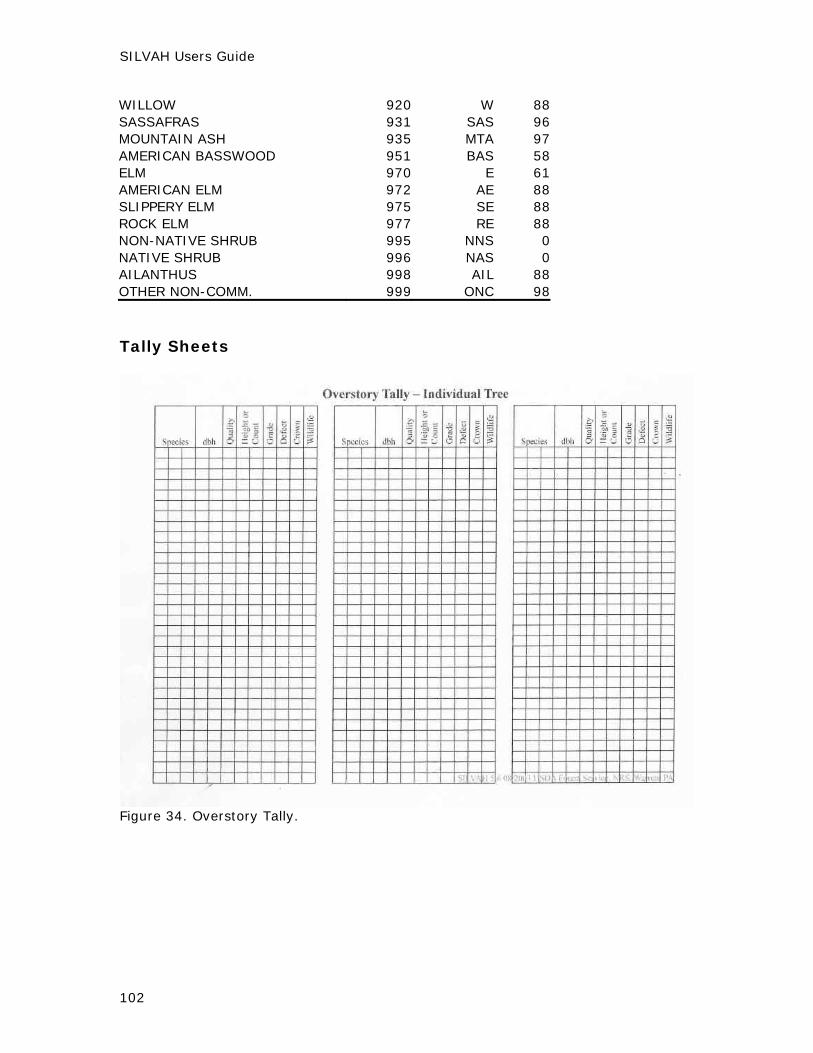
SILVAH Users Guide
WILLOW 920 W 88SASSAFRAS 931 SAS 96MOUNTAIN ASH 935 MTA 97AMERICAN BASSWOOD 951 BAS 58ELM 970 E 61AMERICAN ELM 972 AE 88SLIPPERY ELM 975 SE 88ROCK ELM 977 RE 88NON-NATIVE SHRUB 995 NNS 0NATIVE SHRUB 996 NAS 0AILANTHUS 998 AIL 88OTHER NON-COMM. 999 ONC 98
Tally Sheets
Figure 34. Overstory Tally.
102
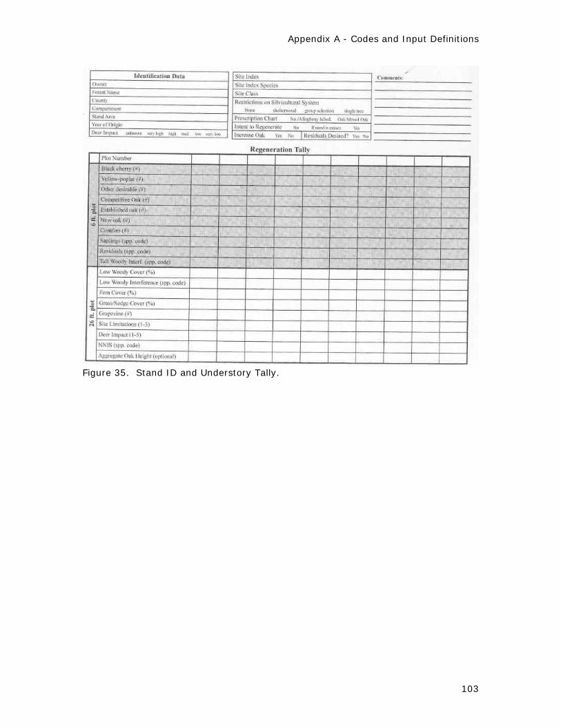
Appendix A - Codes and Input Definitions
103
Figure 35. Stand ID and Understory Tally.


Index
A Accessibility ...............................91 Acreage in Stand .................... 21, 92 Adding Stands Together.................. 7 Alternative Cut...........................58 Aquatic Features In Stand ........ 21, 93 Aquatic Features Within One Mile ...21,
93 Aspect................................... 21, 92 B BAF/Plot Size.......................... 19, 89 Batch Mode ................................... 6 Batch Mode - Creating a batch job...64 Batch Mode - Running a batch job
...............................................65 Black Cherry Regeneration Tally ......95 Board Volumes .............................75 Build-your-own Cuts......................60 C Checkmark Data ...........................34 Checkmark Regen Tally............ 31, 98 Clearcut Acreage..................... 92, 93 Comments/Remarks ..................88 Compartment ......................... 21, 88 Competitive Oak Regeneration Tally.96 Conifers Regeneration Tally ............96 Converting Older Formats ........ 19, 41 Count (stem count) .....................100 County .................................. 21, 88 Cover Type ............................ 21, 88 Crown Condition .........................101 Cruise Information .................. 19, 88 Cubic Volumes..............................75 Cultivated Acreage .................. 92, 94 Current Working Directory............... 8 Custom Treatments.......................60 Cutting Priority .............................60 D Data Directory............................. 8 Data Entry ............................. 10, 23 Data Files .......................... 8, 18, 81 Database Information ................61 dbh.............................................99 dbh size class codes ................ 19, 89 Dead Trees ............................ 53, 99 Deer Impact Index .............20, 80, 91 Default Commercial Sale Breakpoints
...............................................43
Default Diameters For Volume Calculations...............................44
Default Inventory Settings..............42 Default Log Rule ...........................45 Default Management Values ...........41 Default Operation Mode .................46 Default Output Folders...................45 Default Species Codes ...................49 Default Species Parameters ............50 Defaults File .................................40 Defect .......................................101 Desirable Regeneration ..............95 E Elevation ............................... 21, 92 Entering Regen Data......................32 Entering Tree Data .................. 28, 98 Established Oak Regeneration Tally .96 F Fern............................................97 File Types ................................8, 40 Forest Name........................... 21, 88 Forest Types ................................72 G Getting Started.............................. 5 Grade.................................. 19, 100 Grapevines...................................97 Grass ..........................................97 Growth Projection ................ 61, 62 H Herbicide Treatment References......79 How to Edit Data..................... 10, 12 I Installation...............................7, 16 Interactive Mode.......................6, 55 Interference...............................97 Interfering Vegetation ...............97 Inventory Settings .................. 19, 88 K Keystrokes.................................... 9 L Live Trees .............................. 53, 99 Low Woody Interference ................97 M Management Goals.................. 20, 90 Management Value.....................91 Merchantable Heights ............ 74, 100 Modifying a Standard Treatment 58 N Navigation Keys in TREECALC .....9, 69 Net Volumes.................................76
105

SILVAH Users Guide
106
Non-native Invasive Species 35, 37, 38 O Open Acreage......................... 92, 93 Opening Files ......................... 18, 40 Operability .................................91 Other Desirables Regeneration Tally 95 Output ........................................66 Output Directory ......................... 9 Overstory Cruise Type ............. 19, 89 Overstory Data .............................98 Owner .........................................90 P Prescription ...............................58 Product Tables ...........................56 Q Quality ................................. 28, 99 R Regen Cruise Type .....................89 Regeneration Cruise Type....19, 94, 98 Regeneration Plot Size ............. 19, 94 Reports ................................ 56, 66 Residuals .....................................96 Running SILVAH ................12, 14, 65 S Sapling Regeneration Tally .............96 Saving Files............................ 18, 41 Script Mode..............................6, 62 Seed Source Guidelines .................79 Shortcuts.....................................23 Silvicultural Restrictions ........... 20, 90
Site Limits....................................97 Site Quality ............................ 21, 93 Slope .................................... 21, 92 Species Codes ...................... 47, 102 Species Type Code .................. 19, 47 Species X Diameter Table ...........56 Stand Culture Guidelines................80 Stand ID......................................88 Stand Physiography and Site .... 21, 92 Stand Relative Density Thresholds...73 Stand Size Classes ........................73 Stony Soils...................................98 T Tall Woody Interference .................97 Tally Date ....................................19 Thick Duff ....................................98 Topographic Position................ 21, 92 TREECALC....................................69 U Understory Data Collection .............94 V Value ..........................................77 Viewing Output .............................66 W Wet Soils .....................................97 Wildlife Codes.............................101 Working Directory ....................... 8 Y Year of Origin.............................88 Yellow-poplar Regeneration Tally.....95