silly or pointless things people do when analyzing data: 1
TRANSCRIPT

NHRC 2011 © Bruce Weaver 1
Silly or Pointless Things People Do When
Analyzing Data: 1. Conducting a Test of
Normality as a Precursor to a t-test
Bruce Weaver
Northern Health Research Conference
June 10-11, 2011

NHRC 2011 © Bruce Weaver 2
Speaker Acceptance & Disclosure
I have no affiliations, sponsorships, honoraria,
monetary support or conflict of interest from any
commercial source.
However…it is only fair to caution you that this talk
has not undergone ethical review of any sort.
Therefore, you listen at your own peril.

NHRC 2011 © Bruce Weaver 3
On Sermons and Stats Lectures
This probably applies to stats lectures too, so I’ll
make every effort to keep it snappy
"The secret of a good sermon
is to have a good beginning
and a good ending; and to
have the two as close
together as possible."
— George Burns

NHRC 2011 © Bruce Weaver 4
1) normally distributed with
2) equal variances, and
3) each observation must be independent of
all others.
Now to the serious stuff…
The populations from which the two samples are
(randomly) drawn must be Yes, that looks
familiar.
Statistics textbooks often list the following
assumptions for the unpaired t-test,
usually in this order:

NHRC 2011 © Bruce Weaver 5
Example from a Biostatistics Textbook
1. ―…the observations in each
group follow a normal
distribution.‖
2. ―The standard deviations (or
variances) in the two samples
are assumed to be equal‖
3. ―…independence, meaning that
knowing the values of the
observations in one group tells
us nothing about the
observations in the other group‖

NHRC 2011 © Bruce Weaver 6
1. Normally distributed data: It is
assumed that the data are from a
normally distributed population.
2. Homogeneity of variance: … the
variance should not change
systematically throughout the data.
3. Interval data: Data should be
measured at least at the interval
level.
4. Independence: …behaviour of one
participant does not influence
behaviour of another.
Example from an Applied Stats Textbook:
Assumptions for Parametric Tests
First Edition (2000)

NHRC 2011 © Bruce Weaver 7
Normality Assumption Often Listed First
The assumption of sampling from normally
distributed populations often appears first in the list
This can lead users of statistics to conclude that
normality is the most important assumption
It is not – the independence assumption is by far
the most important one…but I don’t have time to talk
about that today
How unfortunate! It sounds like a
real humdinger of a topic.

NHRC 2011 © Bruce Weaver 8
Some Books Recommend Testing for
Normality Prior to Running a t-test
E.g., Field (2002) says to run a test of normality on
the dependent variable
In an example, he runs the Kolmogorov-Smirnov
test of normality (with Lilliefors correction), and finds
that it is statistically significant
What does that mean?
Who cares?! Did you say
Smirnov? Top me up please!

NHRC 2011 © Bruce Weaver 9
For any test of normality:
H0: Sample is drawn from a normal population
H1: Sample is drawn from a non-normal population
If test of normality is statistically significant (p ≤ .05), you
conclude that the sample is from a non-normal population
If test of normality is not statistically significant (p > .05), you
have insufficient evidence to reject the null hypothesis—so
you proceed as if the population is normal
Interpreting Tests of Normality
This is what Field (2000) found

NHRC 2011 © Bruce Weaver 10
Okay, so what now?
―... we cannot use a parametric
test, because the assumption of
normality is not tenable.‖ (Field
2000, pp. 48-49)
Andy Field
He then recommended using the
Mann-Whitney U test (a rank-
based test) instead of the t-test

NHRC 2011 © Bruce Weaver 11
Recap of Field’s Procedure
Test of
Normality
Assume normality and
use a parametric test
(e.g., independent
groups t-test)
Reject the normality
assumption, and use a
non-parametric test (e.g.,
Mann-Whitney U test)
Not statistically
significant (p > .05)
Statistically
significant (p ≤ .05)

NHRC 2011 © Bruce Weaver 12
Now ho-o-old on
there, Baba-Louie!
Quick-Draw McGraw Baba-Louie
Huh?

NHRC 2011 © Bruce Weaver 13
Let’s not forget
what George Box
said about
normality!
Baba-Louie
Okay..
.
Quick-Draw McGraw

NHRC 2011 © Bruce Weaver 14
No real data are normally distributed
―…the statistician knows…that in
nature there never was a normal
distribution, there never was a
straight line, yet with normal and
linear assumptions, known to be
false, he can often derive results
which match, to a useful
approximation, those found in the
real world.‖ (JASA, 1976, Vol. 71, 791-
799; emphasis added)
George Box
Famous statistician and textbook author—
and son-in-law of Sir Ronald F. Fisher
NHRC 2011 © Bruce Weaver 15
So the populations are
never truly normal, at
least not if you’re
working with real data.
Why is normality
listed as one of the
assumptions then?

NHRC 2011 © Bruce Weaver 16
What the textbooks should say
If one was able to sample randomly
from two normally distributed
populations with exactly equal
variances (and with each score
being independent of all others),
then the unpaired t-test would be an
exact test.
Otherwise, it’s an
approximate test.Yours truly
Obscure statistical curmudgeon from
NW Ontario—no relation to R.F. Fisher.

NHRC 2011 © Bruce Weaver 17
Approximate.
Is that bad?
No, not
necessarily.

NHRC 2011 © Bruce Weaver 18
Another Great Comment from Box
George Box
All models are wrong.
Some are useful.
i.e., they are
approximations!
NHRC 2011 © Bruce Weaver 19
A New Question: Is it Useful?
From this point of view, the important question is not
whether the populations we’ve sampled from are
normal – we know they are not
Rather, the important question is whether the
approximation is good enough to be useful
NHRC 2011 © Bruce Weaver 20
Under what conditions is
the approximation good
enough to be useful?
To answer that, we
need to look more
carefully at how z- and
t-tests really work.

NHRC 2011 © Bruce Weaver 21
How z- and t-tests really work
Numerator = a statistic minus the value of the
corresponding parameter under a true null hypothesis
Denominator = the standard error of the statistic in the
numerator
0statistic - parameter| or
statistic
Hz t
SE
Common format for all z- and t-tests:

NHRC 2011 © Bruce Weaver 22
Example 1: Single-sample t-test
X
Xt
s
Statistic = sample mean
Parameter under a
true H0 = pop. mean
SE of the mean
2
X
s ss
nn (df = n - 1)

NHRC 2011 © Bruce Weaver 23
Example 2: Unpaired t-test
1 2
1 2 1 2
X X
X Xt
s
1 2
2 2
1 2
pooled pooled
X X
s ss
n n
Statistic
Parameter under
True H0
SE of the statistic in
the numerator
(df = n1 + n2 - 2)

NHRC 2011 © Bruce Weaver 24
It is the sampling distribution of the
statistic in the numerator that must be
normal, or at least approximately normal,
in order to have a good test
0statistic - parameter| or
statistic
Hz t
SEI’ll make
a note.
The KEY Point

NHRC 2011 © Bruce Weaver 25
0statistic - parameter| or
statistic
Hz t
SE
The Central Limit Theorem (CLT)
The CLT tells us that as the sample size increases, the
sampling distribution of the statistic converges on a
normal distribution, regardless of the shape of the raw
score distributions
And n does not have to be all that large—see example on
next slide with n = 16

NHRC 2011 © Bruce Weaver 26
An Example with 10,000 Samples
of n = 16 from a Skewed Population
The Population Distribution
Mean = 26.98
SD = 5.62
Distribution of Sample Means
(for samples of n = 16)
Mean = 26.99
SD = 1.39
Pretty darn
close to
normal
Severely
skewed
Close enough for the Normal distribution
to be a useful approximation

NHRC 2011 © Bruce Weaver 27
So in other words, the larger
the sample size, the less
important normality of the
population distribution is, right?
This is
correct, Baba-
Louie!

NHRC 2011 © Bruce Weaver 28
But at the same time, as
the sample size increases,
tests of normality become
more and more powerful.
Tim ―the Stats-Man‖ Taylor & Al
That’s good, isn’t it Quick-
Draw? The more POWER,
the better! Right?

NHRC 2011 © Bruce Weaver 29
Not really so in
this case, Tim.
Pay attention now, Tim.
Quick-Draw is about to make
a very good point.

NHRC 2011 © Bruce Weaver 30
As n increases, normality becomes
less and less important for the
validity of the t-test.
Sample Size
Importance of
Normality for
Validity of the
t-test
As n increases,
the importance
of normality
decreases.
Low High
Low
High

NHRC 2011 © Bruce Weaver 31
But at the same time, tests of
normality become more and
more likely to detect
significant non-normality.
Sample Size
Power to detect
Non-Normality As n increases, the
power to detect
non-normality
increases.
Low High
Low
High

NHRC 2011 © Bruce Weaver 32
Sample Size
Import
ance o
f
Norm
alit
y
Sample Size
Pow
er
to d
ete
ct
Non-
Norm
alit
y
Recap of Quick-Draw’s Point
As n increases:
The importance of normality decreases
The power to detect non-normality increases
At cross-
purposes!

NHRC 2011 © Bruce Weaver 33
And that, my friends, is
why tests of normality
are really quite useless
as precursors to t-tests
or other parametric tests.
Yes, I see what
you mean,
Queeks-Draw.

NHRC 2011 © Bruce Weaver 34
Robustness of the t-test to
Non-Normality of the Populations
Some Examples—Time Permitting
Click Here to Continue
the Presentation
Click Here to Skip
to the Summary

NHRC 2011 © Bruce Weaver 35
Robustness of the t-test to Non-normality
The upcoming figure shows performance of the t-test
when sampling from populations of various non-
normal shapes
Performance is measured by how closely the actual
proportion of Type I errors matches the pre-
determined alpha level – e.g., if you set alpha to .05,
the actual proportion of Type I errors should be close
to .05 for a good test

NHRC 2011 © Bruce Weaver 36
Cochran (1942) suggested allowing a 20% error in
the actual Type I error rate—e.g., for nominal
alpha = .05, an actual Type I error rate between
.04 and .06 is acceptable
Cochran’s criterion is admittedly arbitrary, but other
authors have generally followed it (or a similar
criterion) – so we will apply it here
Cochran’s Criterion for
Acceptable Test Performance

NHRC 2011 © Bruce Weaver 37
Thanks to Gene Glass for
Providing the Upcoming Figure
Gene V. Glass

NHRC 2011 © Bruce Weaver 38
Figure 12.2 from Glass & Hopkins,
Statistical Methods in Education and Psychology , 3rd Edition

NHRC 2011 © Bruce Weaver 39
Figure 12.2 from Glass & Hopkins,
Statistical Methods in Education and Psychology , 3rd Edition
R = rectangular, S = skewed, N = normal, L = leptokurtic, ES
= extreme skew, E-S = extreme negative skew, B = bimodal,
M = multimodal, SP = spiked, T = triangular, π = dichotomous

NHRC 2011 © Bruce Weaver 40
Figure 12.2 from Glass & Hopkins,
Statistical Methods in Education and Psychology , 3rd Edition
The actual proportion of Type I Errors
(over repeated samples)
.05
.01

NHRC 2011 © Bruce Weaver 41
Figure 12.2 from Glass & Hopkins,
Statistical Methods in Education and Psychology , 3rd Edition
Numbers above the bars are the sample sizes; if only one
number appears, both samples were the same size

NHRC 2011 © Bruce Weaver 42
Figure 12.2 from Glass & Hopkins,
Statistical Methods in Education and Psychology , 3rd Edition
Cochran’s criterion of acceptable test performance with
alpha set to .05 = actual Type I error rate of .04 to .06
Three cases where the
actual Type I Error rate falls
outside the range .04 to .06

NHRC 2011 © Bruce Weaver 43
S/S – both populations
skewed
N/S – one population is
normal, the other skewed
R/S – one population is
rectangular, one is skewed
In all 3 cases, n1 = n2 = 5
In all 3 cases increasing the
sample size to 15 (one bar
to the right) results in test
performance that meets
Cochran’s criterion
NHRC 2011 © Bruce Weaver 44
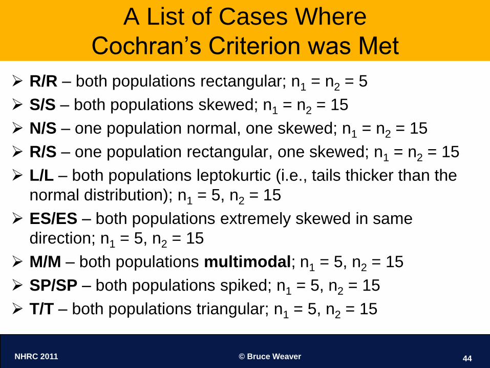
A List of Cases Where
Cochran’s Criterion was Met
R/R – both populations rectangular; n1 = n2 = 5
S/S – both populations skewed; n1 = n2 = 15
N/S – one population normal, one skewed; n1 = n2 = 15
R/S – one population rectangular, one skewed; n1 = n2 = 15
L/L – both populations leptokurtic (i.e., tails thicker than the
normal distribution); n1 = 5, n2 = 15
ES/ES – both populations extremely skewed in same
direction; n1 = 5, n2 = 15
M/M – both populations multimodal; n1 = 5, n2 = 15
SP/SP – both populations spiked; n1 = 5, n2 = 15
T/T – both populations triangular; n1 = 5, n2 = 15

NHRC 2011 © Bruce Weaver 45
Sampling from Dichotomous Populations
Cochran’s criterion (i.e., Type I error rate between
.04 and .06) was also met when samples were
drawn from dichotomous populations with the
following properties:
P = .5, Q = .5, n = 11
P = .6, Q = .4, n = 11
P = .75, Q = .25, n = 11
If P and Q get too extreme (e.g., outside the range .2
to .8), test performance deteriorates
P and Q represent the
proportions falling in
the two categories

NHRC 2011 © Bruce Weaver 46
Summary of Main Points

NHRC 2011 © Bruce Weaver 47
Summary of Main Points (1)
Textbooks list the following assumptions for t-tests:
Sampling from normal populations
Homogeneity of variance
Independence of observations
The normality assumption is often listed first
This leads (some) people to conclude that it is the
most important assumption

NHRC 2011 © Bruce Weaver 48
Summary of Main Points (2)
Some textbook authors recommend using a test of normality
prior to running a t-test – e.g., Field (2000) recommended the
procedure shown below:
Test of
Normality
Assume normality and
use a parametric test
(e.g., independent
groups t-test)
Reject the normality
assumption, and use a
non-parametric test (e.g.,
Mann-Whitney U test)
Not statistically
significant (p > .05)
Statistically
significant (p ≤ .05)

NHRC 2011 © Bruce Weaver 49
Summary of Main Points (3)
But the important thing is normality of the sampling
distribution of the statistic in the numerator of the t-ratio
As the sample size increases, that
sampling distribution converges on the
normal distribution, regardless of
population shape
But at the same time, tests of normality become
more and more powerful – i.e., they are more
and more likely to detect departures from
normality as those departures become less and
less important for the validity of the t-test
Sample Size
Imp
ort
ance
of
Norm
alit
y
Sample Size
Pow
er
to d
ete
ct
Non
-N
orm
alit
y
The Population Distribution
Mean = 26.98
SD = 5.62
Distribution of Sample Means
(for samples of n = 16)
Mean = 26.99
SD = 1.39
Pretty darn
close to
normal
Severely
skewed
Close enough for the Normal distribution
to be a useful approximation
Cross-purposes!

NHRC 2011 © Bruce Weaver 50
Therefore, testing for
normality prior to
running a t-test is rather
silly and pointless.
I agree!
And so…
do we.

NHRC 2011 © Bruce Weaver 51
If not testing for normality, then what?
If means and standard deviations
are sensible and appropriate for
description, then t-tests (or
ANOVA etc) will likely be just fine
for inference.
Yours truly
E.g., reasonably symmetrical
distribution with no outliers
or extreme scores

NHRC 2011 © Bruce Weaver 52
Apologies to Andy Field
Finally, in case Andy Field’s
lawyer is present, let me
point out that the bad advice
about testing for normality
given in Field (2000) does
not appear in the third edition
of the book (Field, 2009).
Third Edition (2009)

NHRC 2011 © Bruce Weaver 53
No animals, cartoon or
real, were harmed
during the production
of this presentation.
A Final Disclaimer

NHRC 2011 © Bruce Weaver 54
Okay…it’s over!
Time to wake up!
Any Questions?

NHRC 2011 © Bruce Weaver 55
Bruce Weaver
E-mail: [email protected]
Tel: 807-346-7704
Go see our posters!

NHRC 2011 © Bruce Weaver 56
References
Cochran WG. The χ2 correction for continuity. Iowa State
College Journal of Science 1942; 16:421–436
Dawson B, Trapp RG. (2004). Basic and clinical Biostatistics (4th
Ed.). New York, NY: Lange Medical Books / McGraw-Hill.
Field A. (2000). Discovering Statistics using SPSS for Windows.
London: Sage.
Field A. (2009). Discovering Statistics using SPSS for Windows
(and sex and drugs and rock ‘n’ roll) (3rd Ed). Los Angeles,
CA: Sage.
Glass GV, Hopkins KD. (1996). Statistical Methods in Education
and Psychology (3rd Ed). Boston, MA: Allyn and Bacon.

NHRC 2011 © Bruce Weaver 57
The Cutting Room Floor

NHRC 2011 © Bruce Weaver 58
The DemTect is a cognitive test designed to detect mild cognitive
impairment and early dementia (Kalbe et al., Int J Geriatr Psychiatry 2004;
19: 136–143)
Summary of
Key Points
Screening for Medically At-Risk Drivers with the SIMARD-MD:
A Failure to Apply the CIHR Knowledge-to-Action FrameworkMichel Bédard, PhD1-3; David B. Hogan, M.D4.; Bruce Weaver, MSc1,2
1. Lakehead University; 2. Northern Ontario School of Medicine; 3. St. Joseph’s Care Group; 4. University of Calgary
Background
•
•
•
Failure to Apply the Knowledge-to-Action Framework
1. British Columbia has adopted the SIMARD-MD for
screening individuals who ―may have cognitive impairment
or dementia that could affect their ability to drive‖.
2. The first step in the CIHR Knowledge-to-Action framework
is synthesis—i.e., systematic review and critical appraisal of
the existing evidence. This requires the existence of multiple
independent studies.
3. Currently, only one published study examines the use of
the SIMARD-MD as it is being implemented in BC. Therefore,
synthesis is not possible, and the CIHR Knowledge-to-Action
Framework has not been followed.
In our view, the findings in this article do not represent the
breakthrough that is claimed.
We see no clear and compelling evidence for superiority of the
SIMARD-MD over other well known cognitive tests
For details, see our forthcoming commentaries in the Journal of
Primary Care & Community Health and the Canadian Geriatric
Journal.
•
•
Relationship Between the SIMARD-MD and DriveABLETM
Currently, there is
only one published
study examining
the SIMARD-MD.
There is nothing to
synthesize. So the BCMA
and the OSMV have
stumbled badly at the first
hurdle in the Knowledge-to-
Action process.
How strong is the evidence in that one study?
•
Declaration of Conflicting Interests
The outcome measure used in the original and validation studies (DriveABLE™ On-Road Evaluation) is part
of the DriveABLE™ Assessment. DriveABLE™ Assessment Centres is a University of Alberta spin-off
company. The CEO and President of DriveABLE™ Assessment Centres, Dr Allen Dobbs, is the spouse of the
first author (B.D.). B.D. has no shares in or financial relationship to DriveABLE™ Assessment Centres. Dr
Allen Dobbs was not involved in this research. D.S. declares no competing interests.
The following is an excerpt from Dobbs & Schopflocher (2010, p. 126). ―At CIHR, knowledge translation (KT) is defined as a
dynamic and iterative process that includes
synthesis, dissemination, exchange and ethically-
sound application of knowledge to improve the
health of Canadians, provide more effective health
services and products and strengthen the health
care system.‖ (emphasis added)
Source: http://www.cihr-irsc.gc.ca/e/39033.html
Definition of Knowledge Translation
Suspected cognitive
impairment that may
affect ability to drive
Screen with
SIMARD-MD
Score ≤ 70
2010 BC Guide in Determining
Fitness to Drive
The 2010 BC Guide in Determining Fitness to Drive is published by
the BC Office of the Superintendent of Motor Vehicles (OSMV)
It can be downloaded from the BCMA website
(https://www.bcma.org/publications-media/handbooks-guides)
The policy rationale section of the Guide begins by questioning the
utility of other well known cognitive tests (e.g., Mini Mental Status
Exam, Trails A and B) for making decisions about fitness to drive.
It concludes by describing the superior properties of the SIMARD-
MD—however, no actual evidence is reported.
•
•
Screening Tool for the Identification
of Medically At-Risk Drivers:
Modification of the DemTect
A for-profit, University of Alberta ―spin-
off‖ company that provides both cognitive
testing and on-road driving assessments( ) ( )
10-word
list recall
Backward
digit span
Number
transcoding*
Word fluency
(Supermarket task)
Delayed recallDemTect(5 tasks)
SIMARD-MD (3 tasks)
* SIMARD-MD uses only
the first two items
The DemTect and the SIMARD-MD
The CIHR Knowledge-to-Action Process
GO SEE OUR POSTER!

NHRC 2011 © Bruce Weaver 59
The Shape of the Sampling Distribution is a
Function of Population Shape and Sample Size
Population Distribution
Non-Normal
Sample Size
Small
Large
The colour in the plot
area represents the
shape of the
sampling distribution
of the statistic
Non-Normal
Normal
Many combinations of
population shape and
sample size result in
the same sampling
distribution shape
Normal

NHRC 2011 © Bruce Weaver 60
Summary of Main Points (3)
But the important thing is normality of the sampling
distribution of the statistic in the numerator of the t-ratio
As the sample size increases, that sampling
distribution converges on the normal
distribution, regardless of population shape
But at the same time, tests of normality become
more and more powerful – i.e., they are more
and more likely to detect departures from
normality as those departures become less and
less important for the validity of the t-test
Sample Size
Imp
ort
ance
of
Norm
alit
y
Sample Size
Pow
er
to d
ete
ct
Non
-N
orm
alit
y
Population Distribution
Non-Normal
Sample Size
Small
Large
Normal

NHRC 2011 © Bruce Weaver 61
Does n have to be ≥ 30?
Some books say that we should (or even must) have n ≥ 30
to ensure that the sampling distribution of the mean is
approximately normal
But the examples shown earlier demonstrate that the
sampling distribution of the mean often becomes nice and
symmetrical with sample sizes much lower than 30
Figure 12.2 from Glass & Hopkins,
Statistical Methods in Education and Psychology , 3rd EditionThe Population Distribution
Mean = 26.98
SD = 5.62
Distribution of Sample Means
(for samples of n = 16)
Mean = 26.99
SD = 1.39
Pretty darn
close to
normal
Severely
skewed
Close enough for the Normal distribution
to be a useful approximation

NHRC 2011 © Bruce Weaver 62
What is the ―rule of 30‖ about then?
In the olden days, textbooks often described inference for
small samples and inference for large samples
E.g., comparing the means of 2 independent samples:
Small samples: independent groups t-test using critical value of t
Large samples: independent groups t-test using critical value of z
From the Standard
Normal Distribution
Often defined as n ≥ 30

NHRC 2011 © Bruce Weaver 63
Why make the distinction?
Why did textbook authors make the distinction between small
and large samples?
Remember that in those days, data analysts used tables of
critical values to determine if a test result was statistically
significant
Tables of critical values take up a lot of room!
When n ≥ 30, the critical value of z (from the Standard Normal
distribution) was judged to be close enough to the critical
value of t that it could be used instead
In older books, tables of critical t-values only go up to df=30
or so

NHRC 2011 © Bruce Weaver 64
Critical value of z
(α = .05, 2-tailed)
After df = 30 (or even 20),
the difference in the critical
values is very small.

NHRC 2011 © Bruce Weaver 65
Back to Stats Class!
Anyone who has taken an introductory stats class no doubt
remembers tackling problems like this:
The birth-weight of newborns
in a particular hospital is
(approximately) normally
distributed with a mean of
3.4 kg and a standard
deviation of 0.6 kg. What
proportion of newborns in
this population have a birth-
weight ≥ 4.5 kg or ≤ 2.3 kg?
Yes, that
looks
vaguely
familiar.

NHRC 2011 © Bruce Weaver 66
Step 1: Sketch the Distribution
3.4 4.0 4.6 5.21.6 2.2 2.8
(Mean)
1, 2 & 3 SD above the mean1, 2 & 3 SD below the mean
ANSWER: Area below 2.3 kg + area above 4.5 kg
2.3 kg 4.5 kg

NHRC 2011 © Bruce Weaver 67
Step 2: Convert to Z-scores
Z = Score – Mean
SD
Z1 = 2.3 – 3.4
0.6 = -1.83
Z2 = 4.5 – 3.4
0.6 = 1.83
Now refer these
values to the
standard normal
distribution.

NHRC 2011 © Bruce Weaver 68
Step 3: Sketch the Standard Normal
Distribution
0.0 1.0 2.0 3.0-3.0 -2.0 -1.0
(Mean)
1, 2 & 3 SD above the mean1, 2 & 3 SD below the mean
Z-score
for 4.5 kg
= 1.83
Z-score
for 2.3 kg
= -1.83Look up area under
the curve in a table, or
use software to find it

NHRC 2011 © Bruce Weaver 69
Step 4 the old fashioned way
Area above 1.83 = .0336
Normal distribution is symmetrical about the mean
Therefore, the area below-1.83 = .0336 too
Therefore, the proportion of newborns having a birth-weight ≥ 4.5 kg or ≤ 2.3 kg is .0336 2 = .0672, or 6.72%
Entry for Z-score
of 1.83 =.0336

NHRC 2011 © Bruce Weaver 70
Step 4 the new-fangled way
Nowadays, one would
probably use software
to obtain the area ≤ Z
= -1.833 plus the area
≥ Z = 1.833
E.g., StaTable from
www.cytel.com
Z = 1.83
Standard
normal
(μ=0, σ=1)
Area ≤ -1.83 plus
area ≥ 1.83 = .06725

NHRC 2011 © Bruce Weaver 71
Why Did That Work?
Z-score problems like that worked because the
distribution of scores was (approximately) normal
In that case, you can transform to Z-scores and refer
to the Standard Normal distribution

NHRC 2011 © Bruce Weaver 72
2 2( ) 2
( )2
Yef y
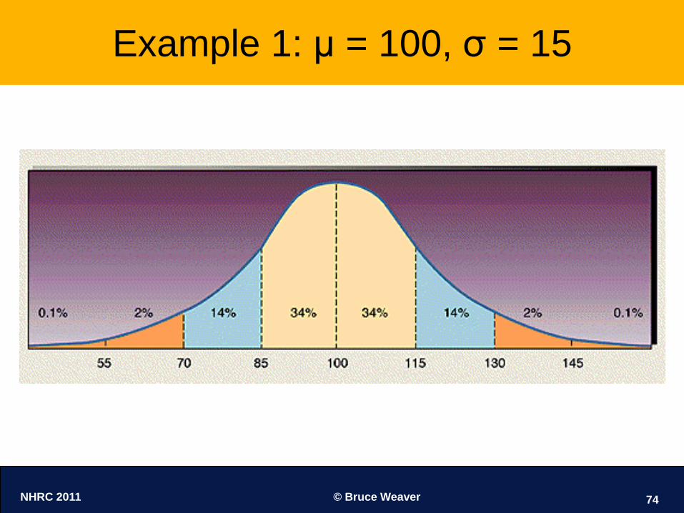
The Normal Distribution
Anyone who has taken an introductory stats course will
remember the Normal (bell-shaped) distribution
Actually, a family of Normal distributions
Mean
Standard
Deviation

NHRC 2011 © Bruce Weaver 73
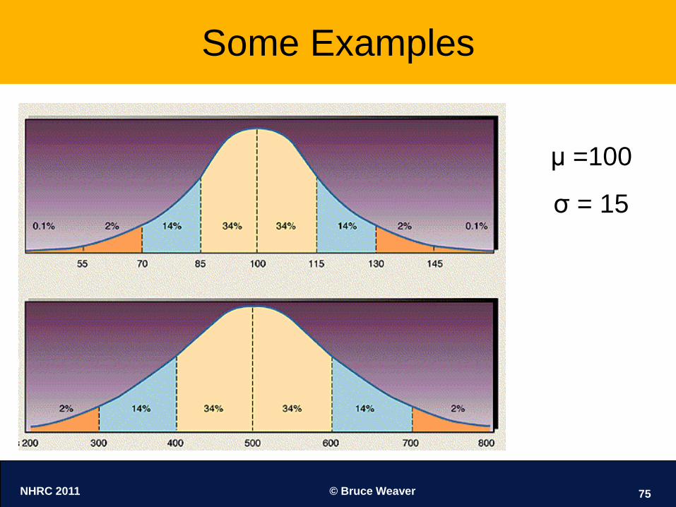
Some Examples
μ =100
σ = 15
NHRC 2011 © Bruce Weaver 74
Example 1: μ = 100, σ = 15
NHRC 2011 © Bruce Weaver 75
Some Examples
μ =100
σ = 15

NHRC 2011 © Bruce Weaver 76
Assumptions for the Unpaired t-test (x)
1. The groups are
independent.
2. The [dependent] variables
of interest are continuous.
3. The data in both groups
have similar standard
deviations.
4. The data is Normally
distributed in both groups.

NHRC 2011 © Bruce Weaver 77
Assumptions for the Unpaired t-test (x)
1. ―…the observations in each
group follow a normal
distribution.‖
2. ―The standard deviations (or
variances) in the two samples
are assumed to be equal‖
3. ―…independence, meaning that
knowing the values of the
observations in one group tells
us nothing about the
observations in the other group‖
NHRC 2011 © Bruce Weaver 78
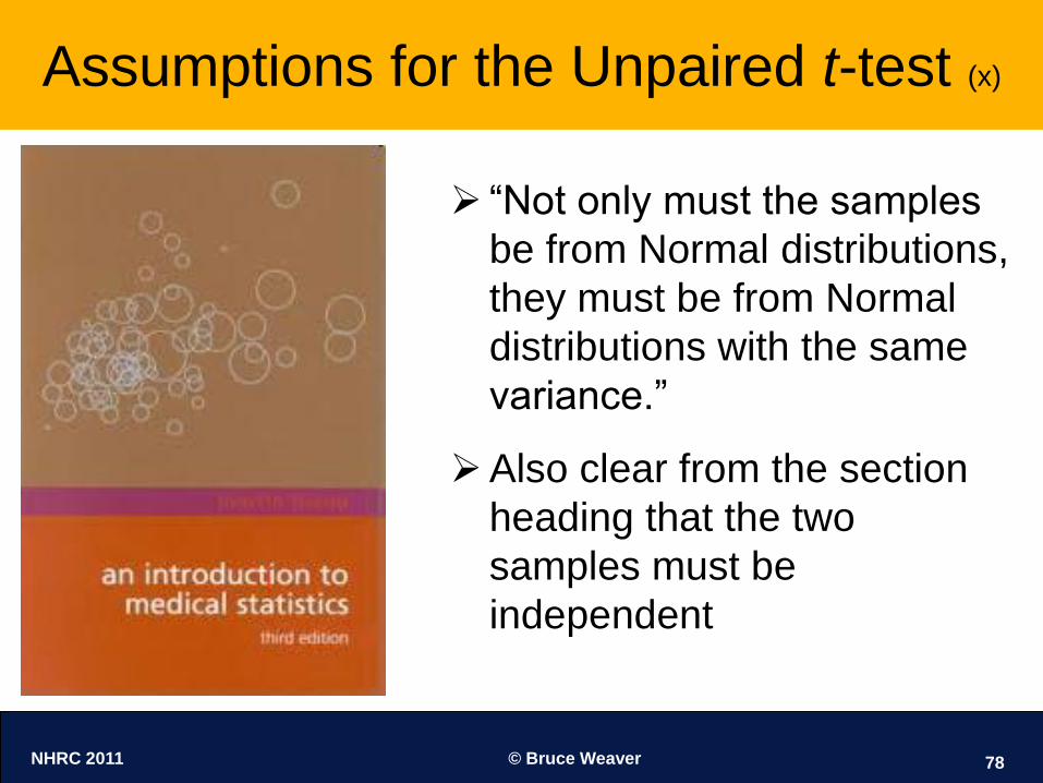
Assumptions for the Unpaired t-test (x)
―Not only must the samples
be from Normal distributions,
they must be from Normal
distributions with the same
variance.‖
Also clear from the section
heading that the two
samples must be
independent

NHRC 2011 © Bruce Weaver 79
How z- and t-tests really work (2)
If the population SE is known, this ratio = Z, and the
standard normal distribution can be used
If the population SE is not known, it must be estimated
(using the sample standard deviation)
In that case, ratio = t, and its sampling distribution is a t-
distribution with appropriate degrees of freedom (df)
0statistic - parameter| or
statistic
Hz t
SE

NHRC 2011 © Bruce Weaver 80
How z- and t-tests really work (3)
Single-sample z-test
X
X
Xz
Statistic
Parameter under
True H0
SE of the statistic in
the numerator
2
X nn

NHRC 2011 © Bruce Weaver 81
Exact vs. Approximate Tests
A test is exact if the sampling distribution of the test statistic is
given exactly by the mathematical distribution used to obtain
the p-value
E.g., the binomial distribution gives exactly the sampling
distribution of X (the number of Heads) in coin-flipping
experiments
A test is approximate if the mathematical distribution only
approximates the true sampling distribution of the test
statistic
E.g., chi-square tests are approximate tests

NHRC 2011 © Bruce Weaver 82
Back to the Assumptions
As we’ve seen, textbooks often list the assumptions
for a t-test as something like this:
1. The data must be sampled from a normally distributed
population (or populations in case of a two-sample test).
2. For two-sample tests, the two populations must have
equal variances.
3. Each score (or difference score for the paired t-test) must
be independent of all other scores.

NHRC 2011 © Bruce Weaver 83
The First Two Assumptions are Never Met
1. As Box noted, nothing in nature is truly normal
2. Furthermore, it is virtually impossible for two different
populations to have variances that are identical down to the
last decimal place.
Therefore, no one who is working with real data meets the
assumptions of normality and homogeneity of variance.
Oh dear!

NHRC 2011 © Bruce Weaver 84
Okay…it’s over!
Time to wake up!
Any Questions?