signature system final report
TRANSCRIPT

Signature System Final Report
Team 5 Luke Bowen
Matt Cieloszyk Rob Gillette
Final Report April 28, 2004
Rensselaer Polytechnic Institute
i
Abstract
The purpose of this report is to detail the design and development of the Signature
System. This report thoroughly examines our system’s motivations, applications, and
specifications. Our objectives and functionality are discussed along with the professional and
societal context of our system.
This report presents a design strategy covering the entire developmental lifecycle of the
system. Progress is then examined including parameter identification, analytical modeling and
model verification. Control design is discussed and results are presented. The system’s cost
structure and timetable have been compiled and presented in an effort to fully define the scope of
the Signature System. The report ends with a discussion of achievements and possible
enhancements to the system
ii

Table of Contents 1. Introduction 1 2. Objectives 3 3. Specifications 5 4. Design Strategy 7 5. Discussion of Progress 5.1 Mechanical Design Phase 8 5.1a Encoders 8 5.1b Pen Mount 8 5.1c Writing Surface 9 5.2 Simulation and Modeling Phase 10
5.2a Validation of Motors 10 5.2c Friction Identification 11 5.2d Open Loop Model 20 5.2c Closed Loop Model
5.3 Control Design Phase 21
6. Discussion of Results 27 7. Tolerance Analysis 31 8. Schedule 32 9. Cost Structure 34 10. Discussion of Achievements 36 11. Possible Enhancements 37 12. Contributions Statement 39 13. Works Cited 40 14. Appendices 41
iii
List of Figures Figure 1: Motor Feasibility Analysis 10 Figure 2: Filtered and Unfiltered Velocities 12 Figure 3: Pan Velocity Curves 13 Figure 4: Pan Friction Identification 14
Figure 5: Tilt Velocity Curves 15 Figure 6: Tilt Friction Identification 16 Figure 7: Pan Axis Model Verification 19 Figure 8: Tilt Axis Model verification 19 Figure 9: Simulink Model of Closed Loop System 20 Figure 10: Pan Axis Controller Root Locus 22 Figure 11: Pan Axis Step Response 22 Figure 12: Tilt Axis Controller Root Locus 23 Figure 13: Tilt Axis Step Response 23 Figure 14: Pan Axis PID Controller Root Locus 24 Figure 15: Pan Axis Step Response with PID 24 Figure 16: Tilt Axis PID Controller Root Locus 25 Figure 17: Tilt Axis Step Response with PID 25 Figure 18: Desired vs. Actual Positions for Square Pattern. 27 Figure 19: Desired vs. Actual Positions for Star Pattern 28 Figure 20: Desired vs. Actual positions for Circle Pattern 29 Figure 21: Desired vs. Actual positions for Signature Pattern 30
iv

List of Tables
Table 1: Design Strategy Showing Dependencies 7 Table 2: Model Coefficient Values 18 Table 3: Schedule and Organization of Labor 32 Table 4: Signature System Cost Structure 34
v

Introduction
Robots are becoming more prevalent in the world today; they are used in all different kinds
of tasks where perfect repetition is needed. For the robot to be useful it needs to be completely
automated and able to handle any disturbances that it encounters. One good example of this is in
the auto industry where robots are used on the assembly lines to weld many parts of the car.
When completing this task they must trace out a predetermined path perfectly in order to produce
a superior weld.
Another scenario where robots track a path is when they are used for painting. Robotic arms
are used to trace out a path so the paint will be flawlessly transferred to the object. Once again it
is important that the controller used can handle any disturbances that it encounters so the paint
correctly applied.
Using these examples of robots tracing out paths, we came up with a similar project. We will
use our simplified robot, the pan-tilt device, to trace out a signature that has been loaded into our
system. On the pan-tilt device will be mounted a spring-loaded pen connected to a solenoid.
This will allow for non-continuous path tracking, such as when an “i” is dotted or a “t” crossed.
Also spring loading the pen allows the canvas to be flat and a larger area to be covered by the
pen.
One real world example that is closely resembles our system is a machine that is sold by
Automated Signature Technology [1]. This unit will take you signature as an input and copy it
perfectly onto anything. This machine can be used by CEOs, presidents, congressmen, or
1

anyone that needs to sign many different documents. Automated Signature Technology claims
that their machines are widely used for these proposes. Our signature system will be a basic
model of similar systems that are used in industry today. However, our system is somewhat
unique due to the pan and tilt degrees of freedom. Products on the market today do not make use
of this type of motion.
2

Objectives
The purpose of the Signature System project is to take an initial pan-tilt structure and create a
machine that can quickly and accurately reproduce text and symbols inputted to the machine.
Using the base machine from Team 4 from the previous semester, we plan on adding equipment
and our own code to achieve the desired results.
We wish to design and develop a machine that is both fully functional and unique. Our
system will be durable, reliable, and cost effective. The Signature System will have possible
market value and fill a vacant niche in the high tech market. Finally, through the development of
the Signature System, we will experience a broad range of engineering disciplines while keeping
the primary focus within the scope of Control Systems Design.
The Signature System will require several simple physical additions consisting of a pen, a
pen mount, and a writing surface. A full analytical model will be developed to aid in control
design. A control system will be developed to allow for the accurate responses to the inputs to
the system. The inverse kinematics will be used in determining the precise location of the pen
tip in relation to the pan and tilt angles.
Consideration was placed on the limited scope of our available time and monetary resources,
and due to these factors our machine will take input via manual entry rather than an automated
process. Our initial plan was to have characters input into the machine by way of an optical
scanning device, but the complexity of the device itself might have proven too costly to include
in the machine.
3

Within our machine several physical characteristics will be prevalent, friction being the most.
Friction will play a major factor in determining the speed of the pen when in contact with the
paper as well as the normal friction incurred through the motions of the axes. For our machine to
accurately duplicate the input, the speed and pressure of the pen onto the writing surface will
need to be adjusted on a real time basis. Using the friction values obtained through
experimentation, our control system will be able to successfully compensate for friction incurred
by the machine.
All the physical components required for our system are easily attainable, which makes
construction and repair easy and cost effective. The system’s only foreseeable mechanical
problem should come from wear and tear. The machine will not move too fast or in abrupt
motions, therefore making the lifespan of all the parts longer. The machine is lightweight and
requires only a standard electric power source, which produces very little negative impact on the
environment. In the social environment, our machine will be very user friendly with minimal
input needed from the user other than the desired output. Also, because of the limited range of
motion and slow speed, the user is put in no danger of injury by being near the machine. From a
business standpoint, there are not many current marketed signature machines. The lack of
competition will allow our machine to enter the market, and with its competitive production
prices have the opportunity to succeed. The Signature System should be able to create a positive
reputation for functionality, product quality, and performance.
4
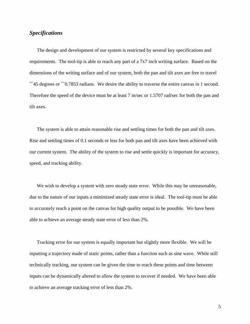
Specifications
The design and development of our system is restricted by several key specifications and
requirements. The tool-tip is able to reach any part of a 7x7 inch writing surface. Based on the
dimensions of the writing surface and of our system, both the pan and tilt axes are free to travel
+/-45 degrees or +/-0.7853 radians. We desire the ability to traverse the entire canvas in 1 second.
Therefore the speed of the device must be at least 7 in/sec or 1.5707 rad/sec for both the pan and
tilt axes.
The system is able to attain reasonable rise and settling times for both the pan and tilt axes.
Rise and settling times of 0.1 seconds or less for both pan and tilt axes have been achieved with
our current system. The ability of the system to rise and settle quickly is important for accuracy,
speed, and tracking ability.
We wish to develop a system with zero steady state error. While this may be unreasonable,
due to the nature of our inputs a minimized steady state error is ideal. The tool-tip must be able
to accurately reach a point on the canvas for high quality output to be possible. We have been
able to achieve an average steady state error of less than 2%.
Tracking error for our system is equally important but slightly more flexible. We will be
inputting a trajectory made of static points, rather than a function such as sine wave. While still
technically tracking, our system can be given the time to reach these points and time between
inputs can be dynamically altered to allow the system to recover if needed. We have been able
to achieve an average tracking error of less than 2%.
5

The Signature System can operate in a point-to-point fashion or in a trajectory tracking
fashion, however the primary application of the system is trajectory tracking. Trajectory inputs
to the system are developed through encoder readings. The user moves the pen through the
motions of his or her signature while both a position and a time log are recorded. The system
reads the position log, at a speed dictated by the time log, and is able to recreate the signature.
The position logs are in radians and are recorded at a sampling time of 0.01 seconds.
6

Design Strategy TABLE 1: DESIGN STRATEGY SHOWING DEPENDENCIES
Simulation and Modeling Phase Control Design Phase Mechanical Design Phase
MATLAB and Solidworks modeling.
Design and construction of pen mounting subsystem.
MATLAB and Simulink simulation.
Development of trajectory calculation methods
Design and construction of writing surface subsystem.
Simulation complete. Design of controller using SISO tools.
Mounting of subsystems.
Tuning of controller on closed loop model.
Replace encoders for better accuracy and reliability.
Tuning of controller on physical system.
Assembly of physical system complete.
System complete and operational.
Table 1 above outlines our generalized design strategy. All work related to the design and
development of the Signature System can be viewed as one of three phases: Simulation and
Modeling Phase, Control Design Phase, or Mechanical Design Phase. The three phases were
undertaken simultaneously however there are some dependencies both between phases and
within each phase. The following sections of this report detail the progress achieved in the
development of the Signature System and are organized into the three phases above.
7

Mechanical Design Phase
Physical creation and adjustment of the machine was completed in the mechanical design
phase. The first physical change made to the machine was the replacement of the existing
encoders from Team 4 last year. When the original encoders were used, the counts produced
were inaccurate. The output received from the encoders showed that they missed counts when
the motors were run at middle to high velocities. To go along with the missed counts, the
location of the encoders on the motor shaft made it so that the output did not take into account
deformation or disturbances incurred when the system was running. In addition, the location
necessitated a conversion of the received data to come up with the correct numbers that took into
account the external gear ratio. When the old encoders were removed and the new ones added,
we relocated them to the output shaft. Once the new encoders were in place the count problem
was found to be fixed, and in addition our resolution was doubled from 1024 to 2048 bits.
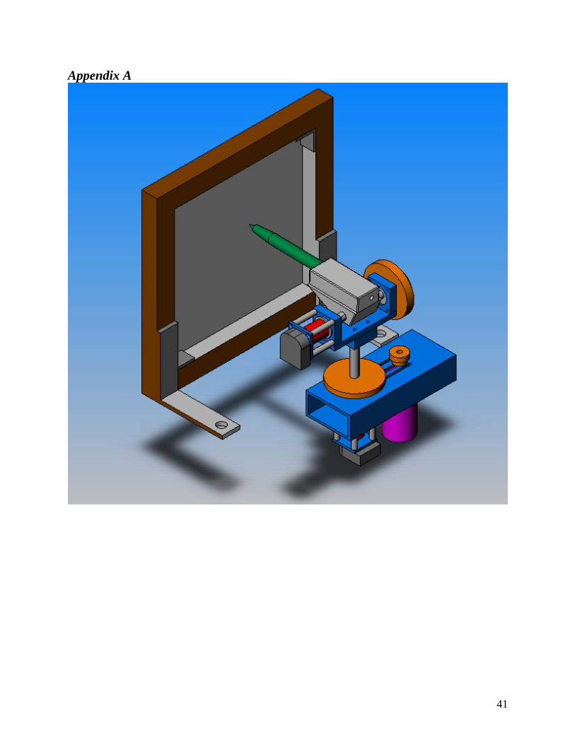
The next step in the mechanical phase was the creation of the pen mount system. The goal of
the pen mount system is to first hold the writing instrument, and secondly to allow the writing
instrument to move forward and back while attached to the tilt axis of the system. Our design
called for using a Sharpie pen since it can write from most any angle and produces a strong and
consistent output. Using an aluminum block as the starting point, the mount was machined with
a hole for the pen and angled underneath to allow for a wide range of motion once attached to the
system. Extra material was then removed to make the piece lighter and less of a load for the
motors. Once mounted, the pen would slide out of the mount when in the lowered position. To
remedy this, a nail was placed in the back of the pen to limit its motion. A spring was also
inserted between the back of the pen and the mount to provide resistance to the pen and ensure
8

constant contact with the writing surface. In the design of the pen mount, an accommodation
was put in place allow for the future addition of a servo to replace the spring and nail. The servo
would pull and push the pen onto the writing surface while being controlled by a MATLAB
script. The final design of the mount can be seen in Appendix A.
The third step in the mechanical phase was the implementation of the writing surface. The
writing surface is created from 1” x ¾ “ wood and a dry erase board. Originally, it was thought
that a dry erase marker could be used, but no marker found would produce an output as
consistent as the Sharpie. Therefore, the Sharpie was used in conjunction with a thick paper
taped to the surface of the dry erase board. Mounts at the bottom of the frame were at first used
to secure the writing surface in place, but during experimentation, it was found that a locked
frame caused imperfect output at extreme pen angles as well as too much friction in the center.
By removing the clamps on the brackets and allowing the writing surface to freely rock back and
forth, the pen was able to consistently write at the extreme angles and reduce the extreme
stresses in the middle.
9

Simulation and Modeling Phase
Validation of Motors
Using MATLAB and Simulink we have been able to verify that the Pittman GM8724S017
motors that we received will be adequate for our system’s requirements. Based on representative
point-to-point inputs and a preliminary PD controller, torque and speed requirements are both
met by the existing motors. Results can be seen in Fig. 1 below.
Fig. 1. Motor feasibility analysis
10
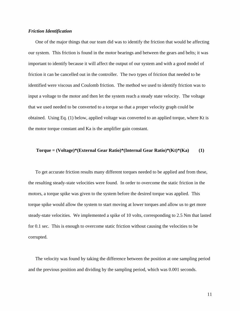
Friction Identification One of the major things that our team did was to identify the friction that would be affecting
our system. This friction is found in the motor bearings and between the gears and belts; it was
important to identify because it will affect the output of our system and with a good model of
friction it can be cancelled out in the controller. The two types of friction that needed to be
identified were viscous and Coulomb friction. The method we used to identify friction was to
input a voltage to the motor and then let the system reach a steady state velocity. The voltage
that we used needed to be converted to a torque so that a proper velocity graph could be
obtained. Using Eq. (1) below, applied voltage was converted to an applied torque, where Kt is
the motor torque constant and Ka is the amplifier gain constant.
Torque = (Voltage)*(External Gear Ratio)*(Internal Gear Ratio)*(Kt)*(Ka) (1)
To get accurate friction results many different torques needed to be applied and from these,
the resulting steady-state velocities were found. In order to overcome the static friction in the
motors, a torque spike was given to the system before the desired torque was applied. This
torque spike would allow the system to start moving at lower torques and allow us to get more
steady-state velocities. We implemented a spike of 10 volts, corresponding to 2.5 Nm that lasted
for 0.1 sec. This is enough to overcome static friction without causing the velocities to be
corrupted.
The velocity was found by taking the difference between the position at one sampling period
and the previous position and dividing by the sampling period, which was 0.001 seconds.
11

Because of the noise in the system, the final velocity numbers had to be filtered so an accurate
steady-state velocity could be found. The filter we used was a 10th order Butterworth filter with
a Wn, natural frequency, of 0.05. This filter was realized through a simple trial and error
approach.
Fig. 2. The left picture is the unfiltered velocity that was calculated from the system. The graph on the right it after the velocity has been filtered using a 10th order Butterworth filter.
As Fig. 2 shows, the filter considerably improved the velocity plots. To find the steady-state
velocity we needed to take the average of the last five thousand samples to ensure that all small
errors would be removed. All of these steps were placed in a MATLAB script that ran with our
Simulink diagram. The voltage range that was used was from -1 to +1 volts, -0.25 Nm to 0.25
Nm; this ensured that enough steady-state velocities were found in order to get a proper
estimation of friction. To make the velocity graphs smoother, and to improve clarity, we used a
polynomial regression on the filtered data that completely smoothes the graphs and makes the
data very clear. In several of the graphs, velocities do not appear to reach steady-state values.
This is due to the polynomial regression. The regression line loses its accuracy and diverges
12

from the data at its tail due to the order of the polynomial. Our velocities all reached a clear
steady-state value.
In order to find the viscous and Coulomb friction, the steady-state velocities needed to be
plotted against the inputted torques. Figures 3 and 4 show the velocities and frictions for the pan
axis, while Figs 5 and 6 show the same information for the tilt axis.
0 5 10 15 20 25-10
-8
-6
-4
-2
0
2
4
6
8
10
time
Vel
ocity
Pan Velocity Curves
Fig. 3. This is a graph of the different steady-state velocities, in rad/sec, for the pan axis acquired from inputting different torque into the system
13
.
-10 -8 -6 -4 -2 0 2 4 6 8 10-0.4
-0.3
-0.2
-0.1
0
0.1
0.2
0.3
steady state theta dot (rad/s)
appl
ied
torq
ue (N
-m)
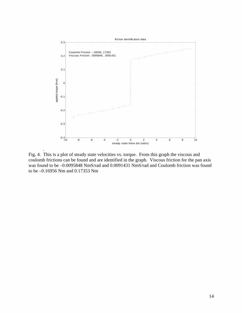
friction identification data
Coulomb Friction: -.16056,.17353Viscous Friction: .0095845, .0091431
Fig. 4. This is a plot of steady state velocities vs. torque. From this graph the viscous and coulomb frictions can be found and are identified in the graph. Viscous friction for the pan axis was found to be –0.0095848 NmS/rad and 0.0091431 NmS/rad and Coulomb friction was found to be –0.16956 Nm and 0.17353 Nm
14

0 5 10 15 20 25-10
-8
-6
-4
-2
0
2
4
6
8
10
tim e
velo
city
Tilt Veloc ity Curves
Fig. 5. This is a graph of the different steady-state velocities for the tilt axis acquired from inputting different torque into the system
15

-10 -8 -6 -4 -2 0 2 4 6 8 10-0.25
-0.2
-0.15
-0.1
-0.05
0
0.05
0.1
0.15
0.2
0.25
steady state theta dot (rad/s)
appl
ied
torq
ue (N
-m)
friction identification data- Tilt Axis
Coulomb Friction: -0.14386,0.15802Viscous Friction: 0.0061749,0.0048541
Fig. 6. This is a plot of steady state velocities vs. torque for the tilt axis. From this graph the viscous and Coulomb frictions can be found and are identified in the graph. Viscous friction for the tilt axis was found to be –0.0061749 NmS/rad and 0.0048541 NmS/rad and Coulomb friction was found to be –0.14386 Nm and 0.15802 Nm. The data points that are not zero need to be fitted with a linear regression so that proper
friction could be found. This was done in a MATLAB script that calculated the line and its
slope, viscous friction, and where it crossed the x-axis, Coulomb friction. Both the positive and
negative values for these frictions are shown on the graphs.
Open Loop Model
Using the data gathered by the torque input test, the full open loop model was determined.
This was done using the equation for the single joint model that we are using to model both the
pan and the tilt joints.
16

(2)
In the Eq. (2) above, the a1 term is for viscous friction, a2 for Coulomb friction, a3 is an
input constant, and a4 is for the gravitational load [2]. Only the tilt axis will be affected by
gravity because it is the only axis that will not keep its position when the power to the system is
shut off. In Eq. (2), theta can be measured from the encoder and from this data both theta-dot
and theta-double-dot can be found. That means that the only variable is the voltage, so by
varying the voltage we can have all the data needed to find a1 through a4. The same data that
was used to find the friction values was plugged into the matrices in Eq. (3) below, so the
coefficients could be found [2]. The resulting values can be found in Table 2.
(3)
17

TABLE 2: MODEL COEFFICIENT VALUES
Pan Joint Tilt Joint
A1 – Viscous Friction Constant 2.34 2.35
A2 – Coulomb Friction Constant .997 .807
A3 – Input Gain Constant 21.08 31.08
A4 – Gravitational Load Constant 0.00 1.8
Once these values were found, a double integrator system was developed in MATLAB to test
the model. The input to this system is a torque and its output is the position of the simulated
system. The velocity was fed back using the above values as gains to system. This needed to be
tested to see if the output to the model would be similar to the output of the actual system.
Different input torques were loaded into the model and the velocity output was plotted against
the original velocity plots that were acquired from the actual system. Results can be seen in Fig.
7 and Fig. 8 below. The graphs show that the output from our model is very close to the output
of the actual system. Now that the open loop model is verified, it can be used for the control
design.
18

0 5 10 15 20 25-10
-8
-6
-4
-2
0
2
4
6
8
10
t im e
velo
city
P an M odel V erific at ion
Fig. 7. This plot is of the actual response, blue line, and the model response, red line, for different input torques to the pan joint.
0 5 10 15 20 25-10
-8
-6
-4
-2
0
2
4
6
8
10
t im e
velo
city
Tilt M odel V erific at ion
Fig. 8. This plot is of the actual response, blue line, and the model response, red line, for different input torques to the tilt joint.
19

Closed Loop Model To come up with a proper control for our system a closed loop model with a PID controller
was developed. This model contained all of the dynamics of the system, friction and inertia,
which had been previously found and verified in the open loop model and simply added a
controller to close the loop. This model would take a desired theta as an input, just like the real
system, and would return the actual position of the system. Our goal for the model was to have a
very accurate response with the controller so that we could then transfer the controller directly to
the physical system.
Fig. 9. Simulink model of closed loop system.
Figure 9 above shows the basic model that was used for the control design that follows [3].
The model works with a MATLAB script that sets the various system parameters of our physical
system. In experiments based on step responses and tracking trajectories, the closed loop model
performs quite accurately in comparison with the physical system.
Control Design Phase
20

The completion of the open and closed loop models marked the start of the control design
phase. Using the results of the single decoupled joint models, we determined the transfer
functions for both the pan and tilt joints. These transfer functions can be seen in Eqs (3) and (4)
below. The tilt plant has an unstable pole at 1.8, which is caused by the gravity term, “a4”. The
pan plant however has no unstable poles due to the lack of a gravitational affect on its position.
Gtilt(s) = 31.08 / s2 + 2.34s –1.8 (3)
Gpan(s) = 21.08 / s2 + 2.35s (4)
These plants were imported separately into MATLAB’s SISO design tool, rltool. A
controller was developed to match our requirements based on frequency domain specifications
and a step response generated by the tool. The initial controllers were designed with two poles
and two zeros. These controllers performed very well in simulations. Figures 10 and 11 below
show the root locus, open loop bode, and step response for the initial pan controller. Figures 12
and 13 below show the same information for the tilt controller.
21

Fig. 10. Pan axis controller root locus and open loop bode plots.
Fig. 11. Step response of pan axis with controller shown in Fig 9. Settling time: 0.0756 sec. Rise time: 0.0496 sec.
22

Fig. 12. Tilt axis controller root locus and open loop bode plots.
Fig. 13. Step response of tilt axis with controller shown in Fig 11. Settling time: 0.0638 sec. Rise time: 0.0442 sec.
23

The controllers developed and shown above did meet and exceed our specifications in
simulation however we decided to design new controllers with two zeros and only one pole at
zero, for the purposes of obtaining a controller in the classic PID form. The results for the pan
axis can be seen in Fig. 14 and Fig. 15 below, while the results for the tilt axis can be seen in Fig.
16 and Fig. 17 below.
Fig. 14. Pan axis PID controller root locus and open loop bode.
Fig. 15. Pan axis step response with PID controller. Rise time: 0.0542 sec, Settling time: 0.0959 sec.
24

Fig. 16. Tilt axis PID controller root locus and open loop bode.
Fig. 17. Tilt axis step response with PID controller. Rise time: 0.109 sec, Settling time: 0.0603 sec. The PID controllers performed just as well as the initial controllers with the extra pole. The
controllers obtained from rltool can be seen in Eqs. (5) and (6) below.
Ctilt(s) = 1.683s2 + 4.065s + 1.5 / s (5)
Cpan(s) = 1.275s2 + 3.01s + 1 / s (6)
25

The controllers were then imported to the Simulink models to be used on the physical
system. The controllers needed some tuning of PID gains to obtain an ideal response from the
motors, however the model-based gains were very similar to the final gains used for the system.
The largest changes had to be made to the proportional gains in each case. The model seemed to
underestimate the effects of friction on the system and resulted in an undershoot in the physical
response. Eqs. (7) and (8) represent the final pan and tilt controllers used in the physical system.
Ctilt(s) = 1.2s2 + 55s + 0.88 / s (7)
Cpan(s) = 1.95s2 + 60s + 0.98 / s (8)
26

Discussion of Results To test our system and its controller we ran a test of several different input trajectories. The
first one that we ran was a simple square who’s input consisted of four corner-points. The
system was commanded to these points and the output was logged.
Fig. 18. Desired vs. Actual positions for square pattern.
As Fig. 18 shows the actual response was very close to the desired response. For this point-
to-point input our controller was well within the 1% error specification. The actual written
output of the system can be found in Appendix C. This system was very smooth and all four
points were clearly reached. Another point-to-point input that was used was a five-point star.
The star would be copied three times to check if the results were repeatable. This was important
to check if the system could be run without recalibration.
27

Fig. 19. Desired vs. Actual position for star pattern.
Once again Fig. 19 shows that the controller was very accurate. The points were still reached
after several passes, which shows that the results for our system are accurate and repeatable.
This star output can also be found in Appendix C.
Because a signature will have different curves to it, a sine function needed to be inputted to
the system. A sine wave was given to both the pan and the tilt but the were ninety degrees out of
phase. This would cause a circle to be written by the system.
28

Fig. 20. Desired vs. Actual positions for circle pattern.
As seen in Fig. 20, once again the output of the system was very close to what the desired
output was. The circle can be found in Appendix C.
The last input that we tested was the most important, a signature. The way this trajectory was
generated was by writing with the system and storing the output of the encoders. This was then
inputted back into the system to see if the signature would be accurately reproduced.
29

Fig. 21. Desired vs. Actual Positions for signature pattern.
Figure 21 shows that the desired trajectory was closely followed by our system. In Appendix
C, both the original signature and the system's signature can be found. The graphs show that the
trajectory was matched. This can also be seen by comparing the two signatures.
30

Tolerance Analysis
The most problematic part of our project is the spring loading system. The performance and
responses of this system are nearly impossible to model. There are slight but considerable
deflections throughout the subsystem during operation, which affect the accuracy of the output.
Under normal operating conditions, deflections of the pen can amount to errors of up to ¼ inch.
Another obstacle will be the friction itself; it will be present at all times when our system is
running. Our system presents a problem that is somewhat unique. The tip of the pen will be in
contact with a surface during operation. This introduces forces that are not present in a
freestanding system. The pen subsystem introduces a position-dependant drag due to its contact
with the paper. This drag may be either modeled in the same way as friction and thus cancelled
out, or it can be dealt with as a disturbance to the controller.
Wear and tear may present another problem. The pen mounting system will be under
considerable stresses during operation. This subsystem will have to be watched closely for
deformation and wear.
Finally, possible problem with the motors appeared during testing. We did a feasibility test
on the motors to see if they would be able to run our system. These tests passed so the motors
should be sufficient. However, when the motors run, some straining and oscillation is clearly
audible and in the plots of the motor output this can be seen. This may not be a problem at all,
but if the motors turn out to be burned out or overused, then replacements will need to be secured
before the system can be considered reliable.
31
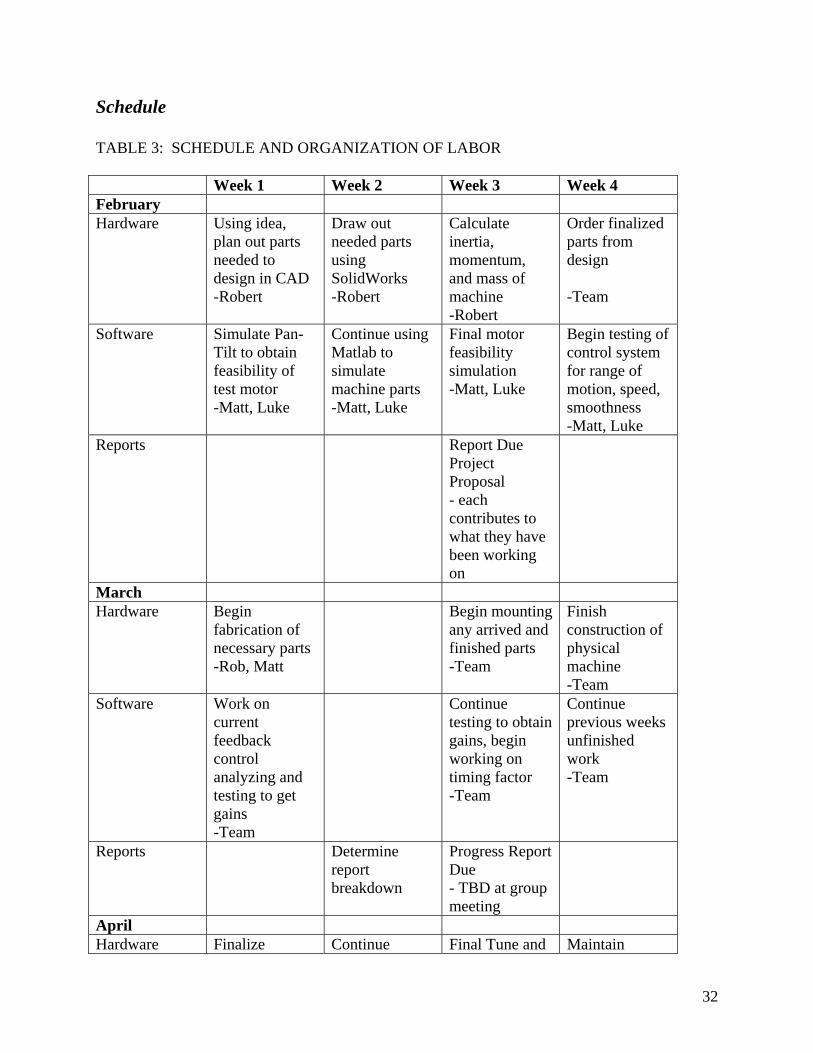
Schedule
TABLE 3: SCHEDULE AND ORGANIZATION OF LABOR Week 1 Week 2 Week 3 Week 4 February Hardware Using idea,
plan out parts needed to design in CAD -Robert
Draw out needed parts using SolidWorks -Robert
Calculate inertia, momentum, and mass of machine -Robert
Order finalized parts from design -Team
Software Simulate Pan-Tilt to obtain feasibility of test motor -Matt, Luke
Continue using Matlab to simulate machine parts -Matt, Luke
Final motor feasibility simulation -Matt, Luke
Begin testing of control system for range of motion, speed, smoothness -Matt, Luke
Reports Report Due Project Proposal - each contributes to what they have been working on
March Hardware Begin
fabrication of necessary parts -Rob, Matt
Begin mounting any arrived and finished parts -Team
Finish construction of physical machine -Team
Software Work on current feedback control analyzing and testing to get gains -Team
Continue testing to obtain gains, begin working on timing factor -Team
Continue previous weeks unfinished work -Team
Reports Determine report breakdown
Progress Report Due - TBD at group meeting
April Hardware Finalize Continue Final Tune and Maintain
32

building and start testing machine -Team
testing and tuning -Team
setup -Team
machine -Team
Software Refine all constants, begin using input for output -Team
Test system -Team
Final adjustments -Team
Tweak Code and control system -Team
Report Team meeting to determine breakdown of report and presentation
Self check-up on report progress
Project Demo -TBD
Final Presentation and Report -Team
Through the semester we used the schedule in Table 3 as a guideline for our progress. In
February, we were able to keep all the set goals in both the hardware and software areas. We
had the CAD drawings and inertias in week two and had tested the motor feasibility by the same
time.
By week three in March, we had fallen slightly behind in the hardware and software phases.
The friction identification went slowly, and the solenoid idea had not progressed. In April, we
looked back picked up the pace of development to catch up to the schedule. Also, at this time we
abandoned the solenoid idea for a servo but still focused mainly on the completion of the control
system.
By week two in April, we were caught up with our set goals, and by the demonstration we
were back on pace. Overall, we were able to achieve our final goal in the mechanical, software,
and report phases.
33

Cost Structure
The cost analysis of our machine theoretically is cost effective given the opportunity to mass-
produce the machine in a final state, but may not be cost effective on a single machine basis.
Due to the common nature of all the machine’s components, competitive pricing will allow for
lower costs and greater profit from the machine production and output. The pieces required for
our machine are shown in Table 4 below.
TABLE 4: SIGNATURE SYSTEM COST STRUCTURE Pan and Tilt Skeleton Item Part Number Price ($) Quantity Total ($) Motor GM8724S017 192.86 2 385.72 Gear A 6A 6-
75NF01812 15.15 2 30.30
Gear A 6A 6-25DF01806
7.76 2 15.52
Timing Belt A6Z16-C01806 1.86 2 3.70 Total 6 434.54 Labor Salary Constant Hours/Week Weeks Employees Total ($) $20 per hour 2.5 10 13 3 19,500.00 The Specifics for This Machine Item Part Number Price ($) Quantity Total ($) Servo Hitec HS 13.02 1 13.02 Standard Sharpie
20206812 3.99 1 (4) 3.99
Screws 823470 2.03 1 (100) 2.03 SolidWorks 3,995.00 1 3,995.00 Matlab 2350.00 2 4700.00 Lab Rental (drill press,
saw) 100/day 5 500.00
Raw Aluminum 3.00 (paid) 1 3.00 Wood 7.00 (paid) 1 7.00 Brackets & Screws
16.30(paid) 1 16.30
Glue 2.00 1 2.00 Total 15 9242.34
34

Pan / Tilt Skeleton Labor Specific Total ($) 434.54 19,500.00 9242.34 29176.88
Besides the cost of materials and labor, there are other considerations to take into account.
The first consideration is the cost of the necessary design and construction equipment. To design
a quality product, design software and a computer are needed. Neglecting the cost of the
computer, assuming that one is already owned, the cost of quality software programs like
SolidWorks and MATLAB can be high. Also, to construct the machine, to save costs it would
be wise to rent out a shop and work until the product makes a name for itself. Including all the
above-mentioned costs, the total for our machine comes to $30051.15. Out of pocket, we have
spent $3.00 on the raw aluminum and $25.30 for wood and brackets for the writing frame.
35

Discussion of Achievements
We feel that we have met the goals that we set forth in the beginning of the semester. Our
machine was well within the specifications that were laid out in the beginning of the report. Our
machine was light, reliable and cheaply built. This was done through a well planned out design
for the hardware and the development of a good model for the software.
At the end of the project our system could accurately reproduce any signature that was
inputted to it. It was able to write over the 7x7 canvas and move to a given point within 1%
error. One part that our team came up short on was the addition of a servo-motor that would be
able to pull the pen back off the canvas. Extensive work was done to get the servo operational,
but with limited time and computers with the A/D converters, we ran out of time. Overall, we
are very please with our project. We met the goals within specifications and we obtained an
accurate output from our machine.
36
Possible Enhancements
The Signature System, while meeting the goals set forth in its proposal, suggests several
possible enhancements or customizations to increase its usefulness.
For the system to offer complete recreation of script, a system could be developed that would
allow the pen to be removed from the writing surface during operation. This would make it
possible, for example, to place the dot above an “i” or cross a “t”. Several possibilities were
explored to complete this function including a servo-motor and an electric pull-type solenoid. It
was determined that a small electric servo would be the best option, allowing a more controlled
stroke rather than the simple on/off operation of a solenoid. Application of the servo is discussed
in Appendix B.
A teaching process could be developed for calculating trajectories rather than directly
recording them. A user could write a series of words or letters and the system could “learn” the
user’s handwriting style and be able to create words that aren’t directly stored in the system. For
example, after the teaching process, a user could enter a keyboard input and the system could
produce the input on paper in the user’s handwriting. Another possible input system that was
briefly considered was a digital writing tablet that could record the user’s input. Trajectories
could be developed through a transformation from pixel coordinates to joint angles.
The writing surface was designed to pivot in order to decrease stresses on the system. The
pivot points were free to rock during operation. While satisfactory for our purposes, this
introduces some uncertainty into the system. The pivot points should be secured with a metal
37

hinge with a light spring to ensure reliability and stability during operation. Also, the writing
surface should be secured to the system itself to ensure an exact and repeatable “home” position.
In addition to these possibilities, several minor physical enhancements could be made to
slightly improve the operation of the system including a more refined pen mount and permanent
encoder connections. These enhancements, while useful and practical, were considered
secondary to the completion of the control and functionality of the Signature System and
therefore were not included in the current system.
38

Contributions Statement
All members of our team contributed equally to the content contained in this report.
Individual contributions are summarized below.
Luke Bowen: Specifications, Control Design Phase, Enhancements, Tolerance Analysis
Matt Cieloszyk: Introduction, Simulation and Modeling Phase, Discussion of Results,
Discussion of Achievements
Rob Gillette: Objectives, Cost, Schedule, Mass Properties ID, CAD work
39
Works Cited [1] Automated Signature Technologies. “SigTech 800” 2003,
< http://www.signaturemachine.com/products/sigtech_800.html >
[2] J. Wen, “Parameter Identification,” class notes for Control Systems Design. ECSE
Department, Rensselaer Polytechnic Institute. Spring 2004
[3] B. Potsaid, “MATLAB/Simuling Overview” class notes for Control Systems Design.
ECSE Department, Rensselaer Polytechnic Institute. Spring 2004
40
Appendix A
41

42

43

44
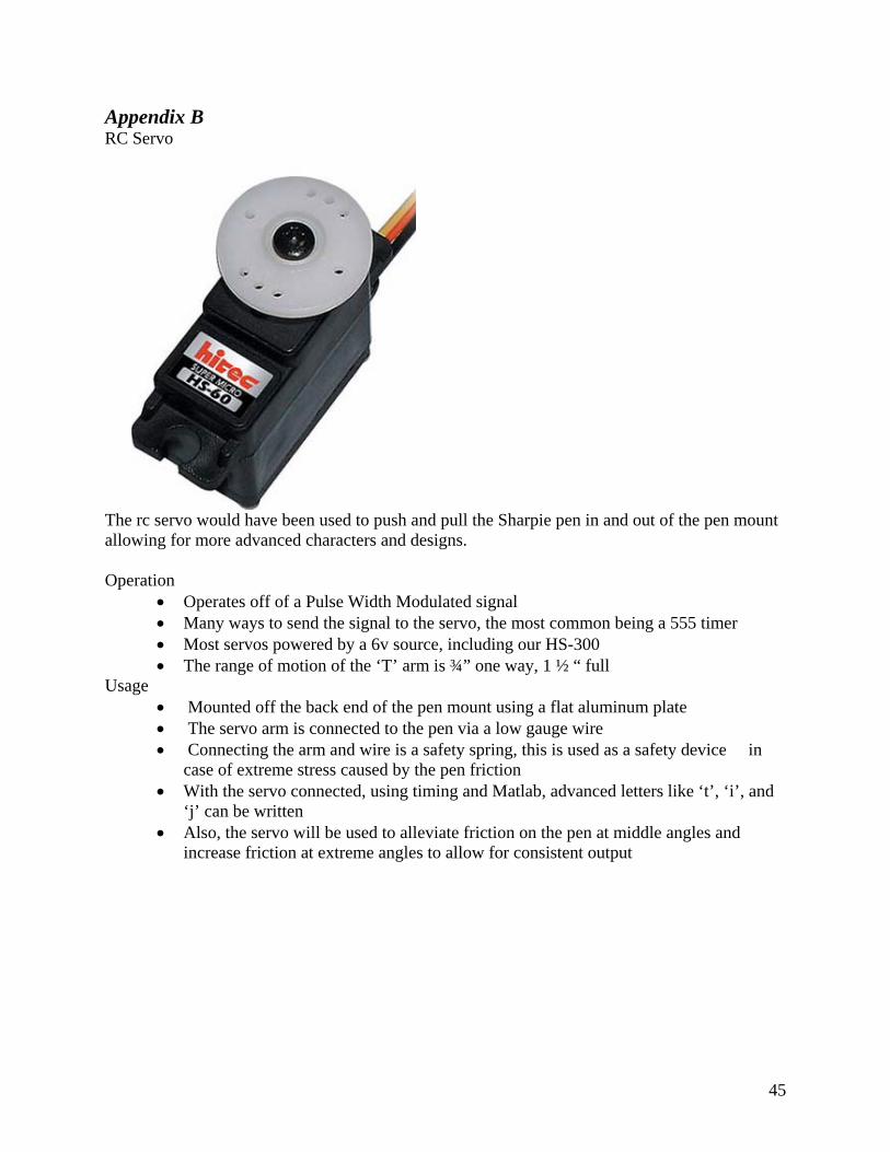
Appendix B RC Servo
The rc servo would have been used to push and pull the Sharpie pen in and out of the pen mount allowing for more advanced characters and designs. Operation
• Operates off of a Pulse Width Modulated signal • Many ways to send the signal to the servo, the most common being a 555 timer • Most servos powered by a 6v source, including our HS-300 • The range of motion of the ‘T’ arm is ¾” one way, 1 ½ “ full
Usage • Mounted off the back end of the pen mount using a flat aluminum plate • The servo arm is connected to the pen via a low gauge wire • Connecting the arm and wire is a safety spring, this is used as a safety device in
case of extreme stress caused by the pen friction • With the servo connected, using timing and Matlab, advanced letters like ‘t’, ‘i’, and
‘j’ can be written • Also, the servo will be used to alleviate friction on the pen at middle angles and
increase friction at extreme angles to allow for consistent output
45

Appendix C
46

47

48

49

50

51