Signaling in Bayesian Stackelberg Games

Haifeng Xu1, Rupert Freeman2, Vincent Conitzer2, Shaddin Dughmi1, Milind Tambe1

1University of Southern California, Los Angeles, CA 90007, USA{haifengx,shaddin,tambe}@usc.edu

2Duke University, Durham, NC 27708, USA{rupert,conitzer}@cs.duke.edu

ABSTRACTAlgorithms for solving Stackelberg games are used in an ever-growing variety of real-world domains. Previous work has ex-tended this framework to allow the leader to commit not only toa distribution over actions, but also to a scheme for stochasticallysignaling information about these actions to the follower. This canresult in higher utility for the leader. In this paper, we extend thismethodology to Bayesian games, in which either the leader or thefollower has payoff-relevant private information or both. This leadsto novel variants of the model, for example by imposing an incen-tive compatibility constraint for each type to listen to the signalintended for it. We show that, in contrast to previous hardnessresults for the case without signaling [5, 16], we can solve unre-stricted games in time polynomial in their natural representation.For security games, we obtain hardness results as well as efficientalgorithms, depending on the settings. We show the benefits of ourapproach in experimental evaluations of our algorithms.

KeywordsBayesian Stackelberg Games, Algorithms, Signaling, SecurityGames

1. INTRODUCTIONIn the algorithmic game theory community, and especially the

multiagent systems part of that community, there has been rapidlyincreasing interest in Stackelberg models where the leader cancommit to a mixed strategy. This interest is driven in part by anumber of high-impact deployed security applications [25]. Oneof the advantages of this framework—as opposed to, say, comput-ing a Nash equilibrium of the simultaneous-move game—is that itsidesteps issues of equilibrium selection. Another is that in two-player normal-form games, an optimal mixed strategy to committo can be found in polynomial time [5]. There are limits to thiscomputational advantage, however; once we extend to three-playergames or Bayesian games, the computational problem becomeshard again [5]. (In a Bayesian game, some of the players haveprivate information that is relevant to the payoffs; their private in-formation is encoded by their type.)

As has previously been observed [4, 28, 23], the leader may beable to do more than commit to a mixed strategy. The leader mayadditionally be able to commit to send signals to the follower(s)

Appears in: Proceedings of the 15th International Conference on Au-tonomous Agents and Multiagent Systems (AAMAS 2016),J. Thangarajah, K. Tuyls, C. Jonker, S. Marsella (eds.),May 9–13, 2016, Singapore.Copyright c© 2016, International Foundation for Autonomous Agents andMultiagent Systems (www.ifaamas.org). All rights reserved.

that are correlated with the action she has chosen. This ability canof course never hurt the leader: she always has the choice of send-ing an uninformative signal. In a two-player normal-form game, itturns out that no benefit can be had from sending an informativesignal. This is because the expected leader utility conditioned oneach signal, which corresponds to a posterior belief of the leader’saction, is weakly dominated by the expected leader utility of com-mitting to the optimal mixed strategy [4]. But this is no longer truein games with three or more players. Moreover, intriguingly, theenriched problem with signaling can still be solved in polynomialtime in these games [4]. The idea of adding signals has also al-ready been explored in security games [28], however these gameswere not Bayesian (but with richer game structure).

In this paper, we extend this line of work to Bayesian Stack-elberg Games (BSGs). We suppose that, when the follower hasmultiple possible types, the leader is able to send a separate signalto each of these types, without learning what the type is. For exam-ple, consider a security game on a rail network in which we aim tocatch ticketless travelers (or, better yet, give them incentives to buya ticket). Here, the attacker’s type could encode at which locationhe starts his journey. Then, by making a separate announcementat each station, we send a separate signal to each type. As an-other example, we may send different signals over different (say)radio frequencies. In this case, each follower type receives a sepa-rate signal depending on the frequency to which he is listening. Inthis latter example (unlike the former), we also require an incen-tive compatibility (IC) constraint: no type should find it beneficialto switch over to a different frequency, since we have no way offorcing a type to listen to a particular frequency.

Besides considering the case of multiple follower types, we alsoconsider the case of multiple leader types. Here, the signal sentby the leader can be correlated with her type as well as her action.Among other examples, this allows us to capture models where theleader is a seller of some item, and the type of the leader corre-sponds to knowledge about, for example, the quality of the item.She can then send an informative (but perhaps not completely in-formative) signal about this quality to the buyer. Such models aresometimes studied in the auction design literature [8, 18, 12], buthere our interest is in generally applicable algorithms.

Our Contributions: We consider signaling in different modelsof Bayesian Stackelberg games, and essentially pin down the com-putational complexity in each. For the case with multiple followertypes (but a single leader type), we show that the optimal combina-tions of mixed strategies and signaling schemes can be computedin polynomial time using linear programming.1 This is the case

1One may wonder whether this just follows from the fact that wecan model Bayesian games by representing each type as a singleplayer, thereby reducing it to a multiplayer game. But this does not

whether an incentive compatibility constraint applies or not. How-ever, for security games, we show that the problem is NP-hard,though we do identify a special case that can be solved efficiently.We also provide hardness evidence that this special case is almostthe best one can hope for in terms of polynomial computability.

For the case with multiple leader types (but a single followertype), we show that the optimal combinations of mixed strate-gies and signaling schemes can also be computed in polynomialtime. Moreover, the polynomial-time solvability extends to secu-rity games in this setting. We note that our results (both hardnessand polynomial-time solvability) can be easily generalized to thecase with both multiple leader and follower types, thus we will notdiscuss it explicitly in the paper. We conclude with an experimentalevaluation of our approach.

2. AN EXAMPLE OF STACKELBERGCOMPETITION

The Stackelberg model was originally introduced to capture mar-ket competition between a leader (e.g., a leading firm in some area)and a follower (e.g., an emerging start-up). The leader has an ad-vantage of committing to a strategy (or equivalently, moving first)before the follower makes decisions. Here we consider a Bayesiancase of Stackelberg competition where the leader does not have fullinformation about the follower.

For example, consider a market with two firms, a leader and afollower. The leader specializes in two products, product 1 andproduct 2. The follower is a new start-up which focuses on only oneproduct. It is publicly known that the follower will focus on product1 with probability 0.55 (call him a follower of type θ1 in this case),and product 2 with probability 0.45 (call him a follower of typeθ2). But the realization is only known to the follower. The leaderhas a research team, and must decide which product to devote this(indivisible) team to, or to send them on vacation. On the otherhand, the follower has two options: either entering the market anddeveloping the product he focuses on, or leaving the market.

Naturally, the follower wants to avoid competition with theleader’s research team. In particular, depending on the type ofthe follower, the leader’s decision may drive the follower out ofthe market or leave the follower with a chance to gain substan-tial market share. This can be modeled as a Bayesian StackelbergGame (BSG) where the leader has one type and the follower hastwo possible types. To be concrete, we specify the payoff matri-ces for different types of follower in Figure 1, where the leader’saction Li simply denotes the leader’s decision to devote the teamto product i for i ∈ {1, 2, ∅}; ∅ means a team vacation. Similarly,the follower’s action Fi means the follower focuses on productsi ∈ {1, 2, ∅} where ∅ means leaving the market. Notice that thepayoff matrices force the follower to only produce the product thatis consistent with his type, otherwise he gets utility −∞. The util-ity for the leader is relatively simple: the leader gets utility 1 onlyif the follower (of any type) takes action F∅, i.e., leaving the mar-ket, and gets utility 0 otherwise. In other words, the leader wantsto drive the follower out of the market.

Possessing a first-mover advantage, the leader can commit to arandomized strategy to assign her research team so that it maxi-mizes her utility in expectation over the randomness of her mixedstrategy and the follower types. Unfortunately, finding the optimalmixed strategy to commit to turns out to be NP-hard for BSGs ingeneral [5]. Nevertheless, by exploiting the special structure in thisexample, it is easy to show that any mixed strategy that puts at least

work, because the corresponding normal form of the game wouldhave size exponential in the number of types.

F∅ F1 F2

L∅ 0 2 −∞L1 0 −1 −∞L2 0 2 −∞

type θ1, p = 0.55

F∅ F1 F2

L∅ 0 −∞ 1L1 0 −∞ 1L2 0 −∞ −1

type θ2, p = 0.45

Figure 1: Payoff Matrices for Followers of Different Types

2/3 probability onL1 is optimal for the leader to commit to. This isbecause to drive a follower of type θ1 out of the market, the leaderhas to take L1 with probability at least 2/3. Likewise, to drive afollower of type θ2 out of the market, the leader has to take L2 withprobability at least 1/2. Since 2/3 + 1/2 > 1, the leader cannotachieve both, so the optimal choice is to drive the follower of typeθ1 (occurring with a higher probability) out of the market so thatthe leader gets utility 0.55 in expectation.

Notice that the leader commits to the strategy without knowingthe realization of the follower’s type. This is reasonable because thefollower, as a start-up, can keep information confidential from theleader firm at the initial stage of the competition. However, as timegoes on, the leader will gradually learn the type of the follower.Nevertheless, the leader firm cannot change her chosen action atthat point because, for example, there is insufficient time to switchto another product. Can the leader still do something strategic atthis point? In particular, we study whether the leader can benefitby partially revealing her action to the follower after observing thefollower’s type. To be concrete, consider the following leader pol-icy. Before observing the follower’s type, the leader commits tochoose action L1 and L2 uniformly at random, each with proba-bility 1/2. Meanwhile, the leader also commits to the followingsignaling scheme. If the follower has type θ1, the leader will send asignal σ∅ to the follower when the leader takes action L1, and willsend either σ∅ or σ1 uniformly at random when the leader takesaction L2. Mathematically, the signaling scheme for the followerof type θ1 is captured by the following probabilities.

Pr(σ∅|L1, θ1) = 1 Pr(σ1|L1, θ1) = 0;Pr(σ∅|L2, θ1) = 1

2Pr(σ1|L2, θ1) = 1

2.

On the other hand, if the follower has type θ2, the leader will alwayssend σ∅ regardless of what action she has taken.

When a follower of type θ1 receives signal σ∅ (occurring withprobability 3/4), he infers the posterior belief of the leader’s strat-egy as Pr(L1|σ∅, θ1) = 2/3 and Pr(L2|σ∅, θ1) = 1/3, thusderiving an expected utility of 0 from taking action F1. Assum-ing the follower breaks ties in favor of the leader,2 he will thenchoose action F∅, leaving the market. On the other hand, if thefollower receives σ1 (occurring with probability 1/4), he knowsthat the leader has taken action L2 for sure; thus the follower willtake action F1, achieving utility 2. In other words, the signals σ∅and σ1 can be viewed as recommendations to the follower to leavethe market (σ∅) or develop the product (σ1), though we emphasizethat a signal has no meaning beyond the posterior distribution onleader’s actions that it induces. As a result, the leader drives thefollower out of the market 3/4 of the time. On the other hand, ifthe follower has type θ2, since the leader reveals no information,the follower derives expected utility 0 from taking F2, and thuswill choose F0 in favor of the leader. In expectation, the leader getsutility 3

4× 1

2+ 1

2= 0.875(> 0.55). Thus, the leader achieves

better utility by signaling.The design of the signaling scheme above depends crucially on

the fact that the leader can distinguish different follower types be-2This is without loss of generality because the leader can alwaysslightly tune the probability mass to make the follower slightly pre-fer F∅.

fore sending the signals and will signal differently to different fol-lower types. This fits the setting where the leader can observe thefollower’s type after the leader takes her action and then signalsaccordingly. However, in many cases, the leader is not able to ob-serve the follower’s type. Interestingly, it turns out that the leadercan in some cases design a signaling scheme which incentivizes thefollower to truthfully report his type to the leader and still benefitfrom signaling. Note that the signaling scheme above does not sat-isfy the follower’s incentive compatibility constraints – if the fol-lower is asked to report his type, a follower of type θ2 would bebetter off to report his type as θ1. This follows from some simplecalculation, but an intuitive reason is that a follower of type θ2 willnot get any information if he truthfully reports θ2, but will receivea more informative signal, thus benefit himself, by reporting θ1.

Now let us consider another leader policy. The leader commitsto the mixed strategy (L∅, L1, L2) = (1/11, 6/11, 4/11). Inter-estingly, this involves sometimes sending the research team on va-cation! Meanwhile, the leader also commits to the following moresophisticated signaling scheme. If the follower reports type θ1, theleader will send signal σ∅ whenever L1 is taken as well as 3

4of

the time that L2 is taken; otherwise the leader sends signal σ1. Ifthe follower reports type θ2, the leader sends signal σ∅ wheneverL2 is taken as well as 2

3of the time that L1 is taken; otherwise

the leader sends signal σ2. It turns out that this policy is incen-tive compatible – truthfully reporting the type is in the follower’sbest interests – and achieves the maximum expected leader utility1722≈ 0.773 ∈ (0.55, 0.875) among all such policies.

Justification of Commitment: The assumption of commitmentto strategies is well motivated, and has been justified, in many ap-plications, e.g., market competition [9] and security [25]. This isusually due to the leader’s first-mover advantage. The assumptionof commitment to signaling schemes is justified on the grounds ofgames that are played repeatedly (e.g., a leading firm plays repeat-edly with start-ups that can show up and fade away), so the fol-lower can learn the signaling scheme - how the signals correlatewith leader actions taken. On the other hand, to balance the shortterm utility and long-term credibility, the leader has incentives tofollow the signaling scheme in order to build a reputation about herstrategy of disclosing information. We refer the reader to [24] formore thorough discussions of this phenomenon.

Remark: This example shows that the additional ability of com-mitting to a signaling scheme can profoundly affect both players’strategies. We study how such additional commitment changes thegame as well as the computation of the leader’s optimal policy. Therest of this paper is organized as follows. In Section 3 we general-ize the above example to BSGs, and also examine its application toBayesian Stackelberg Security Games, a model of growing interestin modeling various security challenges. Note that the above exam-ple only concerned the case where the follower has multiple types.In Section 4, we consider a variant of the model where the leaderhas multiple types (but the follower has only one type), and seek tocompute the optimal leader policy. We show simulation results inSection 5 and conclude in Section 6.

3. SINGLE LEADER TYPE, MULTIPLEFOLLOWER TYPES

3.1 The ModelIn this section, we generalize the example in Section 2 and con-

sider how the leader’s additional ability of committing to a sig-naling scheme changes the game and the computation. We startwith a Bayesian Stackelberg Game (BSG) with one leader type

1

Leader commits (strategy + signaling scheme)

Leader “observes” follower type and samples a signal

Follower’s type is realized

Follower observes the signal and plays

time

Leader plays an action

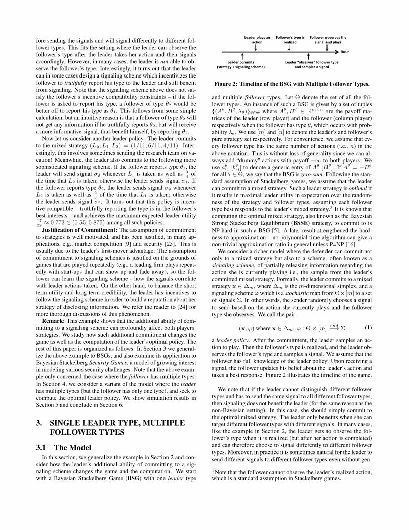
Figure 2: Timeline of the BSG with Multiple Follower Types.

and multiple follower types. Let Θ denote the set of all the fol-lower types. An instance of such a BSG is given by a set of tuples{(Aθ, Bθ, λθ)}θ∈Θ where Aθ, Bθ ∈ Rm×n are the payoff ma-trices of the leader (row player) and the follower (column player)respectively when the follower has type θ, which occurs with prob-ability λθ . We use [m] and [n] to denote the leader’s and follower’spure strategy set respectively. For convenience, we assume that ev-ery follower type has the same number of actions (i.e., n) in theabove notation. This is without loss of generality since we can al-ways add “dummy" actions with payoff −∞ to both players. Weuse aθij [bθij ] to denote a generic entry of Aθ [Bθ]. If Aθ = −Bθfor all θ ∈ Θ, we say that the BSG is zero-sum. Following the stan-dard assumption of Stackelberg games, we assume that the leadercan commit to a mixed strategy. Such a leader strategy is optimal ifit results in maximal leader utility in expectation over the random-ness of the strategy and follower types, assuming each followertype best responds to the leader’s mixed strategy.3 It is known thatcomputing the optimal mixed strategy, also known as the BayesianStrong Stackelberg Equilibrium (BSSE) strategy, to commit to isNP-hard in such a BSG [5]. A later result strengthened the hard-ness to approximation – no polynomial time algorithm can give anon-trivial approximation ratio in general unless P=NP [16].

We consider a richer model where the defender can commit notonly to a mixed strategy but also to a scheme, often known as asignaling scheme, of partially releasing information regarding theaction she is currently playing i.e., the sample from the leader’scommitted mixed strategy. Formally, the leader commits to a mixedstrategy x ∈ ∆m, where ∆m is the m-dimensional simplex, and asignaling scheme ϕwhich is a stochastic map from Θ×[m] to a setof signals Σ. In other words, the sender randomly chooses a signalto send based on the action she currently plays and the followertype she observes. We call the pair

(x, ϕ) where x ∈ ∆m; ϕ : Θ× [m]rnd−→ Σ (1)

a leader policy. After the commitment, the leader samples an ac-tion to play. Then the follower’s type is realized, and the leader ob-serves the follower’s type and samples a signal. We assume that thefollower has full knowledge of the leader policy. Upon receiving asignal, the follower updates his belief about the leader’s action andtakes a best response. Figure 2 illustrates the timeline of the game.

We note that if the leader cannot distinguish different followertypes and has to send the same signal to all different follower types,then signaling does not benefit the leader (for the same reason as thenon-Bayesian setting). In this case, she should simply commit tothe optimal mixed strategy. The leader only benefits when she cantarget different follower types with different signals. In many cases,like the example in Section 2, the leader gets to observe the fol-lower’s type when it is realized (but after her action is completed)and can therefore choose to signal differently to different followertypes. Moreover, in practice it is sometimes natural for the leader tosend different signals to different follower types even without gen-

3Note that the follower cannot observe the leader’s realized action,which is a standard assumption in Stackelberg games.

uinely learning their types, e.g., the follower’s type may be definedby their location, in which case we can send signals using location-specific devices such as physical signs or radio transmission – thisfits our model just as well. We will elaborate one such examplewhen discussing security games.

3.2 Commitment to Optimal Leader PolicyWe first consider the case where the leader can explicitly observe

the follower’s type, and thus can signal differently to different fol-lower types, but this would also fit the location based model. Westart with a simple observation.

OBSERVATION 3.1 (SEE, E.G., [15]). There exists an opti-mal signaling scheme using at most n signals with signal σj rec-ommending action j ∈ [n] to the follower.

Observation 3.1 follows simply from the fact that if two signals re-sult in the same follower best-response action, we can merge thesesignals, resulting in a new signal without changing the follower’sbest response action and the leader’s utility. As a result, for the restof the paper we assume that Σ = {σj}j∈[n].

THEOREM 3.2. The optimal leader policy can be computed inpoly(m,n, |Θ|) time by linear programming.

PROOF. Let x = (x1, ..., xm) ∈ ∆m be the leader’s mixedstrategy to commit to. As a result of Observation 3.1, the signalingscheme ϕ can be characterized by ϕ(j|i, θ) which is the probabil-ity of sending signal σj conditioned on the leader’s (pure) actioni and the follower’s type θ. Then, pθij = xi · ϕ(j|i, θ) is the jointprobability that the leader plays pure strategy i and sends signal σj ,conditioned on observing the follower of type θ. Then the follow-ing linear program computes the optimal leader policy captured byvariables {xi}i∈[m] and {pθij}i∈[m],j∈[n],θ∈Θ.

maximize∑θ∈Θ λθ

∑ij p

θija

θij

subject to∑nj=1 p

θij = xi, for i ∈ [m], θ ∈ Θ.∑m

i=1 pθijb

θij ≥

∑mi=1 p

θijb

θij′ , for θ, j 6= j′.∑m

i=1 xi = 1pθij ≥ 0, for all i, j, θ.

.(2)

The first set of constraints mean that the summation of probabilitymass pθij – the joint probability of playing pure strategy i and send-ing signal σj conditioned on follower type θ – over j should equalthe probability of playing action i for any type θ. The second setof constraints are to guarantee that the recommended action j bysignal σj is indeed the follower’s best response.4

Given any game G, let Usig(G) be the leader’s expected utilityby taking the optimal leader policy computed by LP (2). Moreover,let UBSSE(G) be the leader’s utility in the BSSE, i.e., the expectedleader utility by committing to (only) the optimal mixed strategy.

PROPOSITION 3.3. If G is a zero-sum BSG, then Usig(G) =UBSSE(G). That is, the leader does not benefit from signaling inzero-sum BSGs.

The intuition underlying Proposition 3.3 is that, in a situation ofpure competition, any information volunteered to the follower willbe used to “harm" the leader. In other words, signaling is onlyhelpful when the game exhibits some “cooperative components".We defer the formal proof to the appendix at the end of this paper.

Remark: Notice that computing the optimal mixed strategy (as-suming no signaling) to commit to is NP-hard in general for the4This is often called “obedience".

setting above (even NP-hard to approximate within any non-trivialratio), as shown in [5, 16]. Interestingly, it turns out that when weconsider a richer model with signaling, the problem becomes easy!Intuitively, this is because the signaling scheme “relaxes" the gameby introducing correlation between the leader’s and follower’s ac-tion (via the signal). Such correlation allows more efficient compu-tation. Similar intuition can be seen in the literature on computingNash equilibria (hard for two players [6, 3]) and correlated equilib-ria (easy in fairly general settings [20, 14]).

3.3 Incentivizing the Follower TypeIn many situations, it is not realistic to expect that the leader can

observe the follower’s type. For example, the follower’s type maybe whether he has a high or low value for an object, which is notdirectly observable. In such cases, the leader can ask the followerto report his type. However, it is not always in the follower’s bestinterests to truthfully report his own type since the signal that is in-tended for a different follower type might be more beneficial to thefollower (recall the example in Section 2). In this section, we con-sider how to compute an optimal incentive compatible (IC) leaderpolicy that incentivizes the follower to truthfully report his type,and meanwhile benefits the leader.

We note that Observation 3.1 still holds in this setting. To seethis, consider a follower of type θ that receives more than one sig-nal, each resulting in the same follower best response. Then, asbefore, we can merge these signals without harming the followerof type θ. But if a follower of type β 6= θ misreports his typeas θ, receiving the merged signal provides less information thanreceiving one of the unmerged signals. Therefore, if the followerof type β had no incentive to misreport type θ before the signalswere merged, he has no incentive to misreport after the signals aremerged. So any signaling scheme with more than n signals can bereduced to an equivalent scheme with exactly n signals.

THEOREM 3.4. The optimal incentive compatible (IC) leaderpolicy can be computed in poly(m,n, |Θ|) time by linear program-ming, assuming the leader does not observe the follower’s type.

PROOF. Similar to Section 3.2, we still use variables x ∈ ∆m

and {pθij}i∈[m],j∈[n],θ∈Θ to capture the leader’s policy. Thenαθj =

∑mi=1 p

θij is the probability of sending signal j when the

follower has type θ. Now consider the case where the follower re-ports type β, but has true type θ. When the leader recommendsaction j (assuming a follower of type β), which now is not neces-sarily the follower’s best response due to the follower’s misreport,the follower’s utility for any action j′ is 1

αβj

∑mi=1 p

βijb

θij′ . There-

fore, the follower’s action will be arg maxj′1

αβj

∑mi=1 p

βijb

θij′ with

expected utility maxj′1

αβj

∑mi=1 p

βijb

θij′ . As a result, the expected

utility for the follower of type θ, but misreporting type β, is

U(β; θ) =

n∑j=1

[αβj ×max

j′

1

αβj

m∑i=1

pβijbθij′

]=

n∑j=1

[maxj′

m∑i=1

pβijbθij′

]Therefore, to incentivize the follower to truthfully report his

type, we only need to add the incentive compatibility constraintsU(θ; θ) ≥ U(β; θ). Using the condition maxj′

∑mi=1 p

θijb

θij′ =∑m

i=1 pθijb

θij , i.e., the recommended action j by σj is indeed the

follower’s best response when the follower has type θ, we have

U(θ; θ) =∑nj=1

[maxj′

∑mi=1 p

θijb

θij′]

=∑nj=1

∑mi=1 p

θijb

θij

Therefore, incorporating the above constraints to LP (2) gives thefollowing optimization program which computes an optimal incen-

tive compatible leader policy.

maximize∑θ∈Θ λθ

∑ij p

θija

θij

subject to∑nj=1 p

θij = xi, for all i, θ.∑m

i=1 pθijb

θij ≥

∑mi=1 p

θijb

θij′ , for j 6= j′.∑n

j=1

∑mi=1 p

θijb

θij ≥∑n

j=1

[maxj′

∑mi=1 p

βijb

θij′

], for β 6= θ.∑m

i=1 xi = 1pθij ≥ 0, for all i, j, θ.

(3)Notice that

∑nj=1

[maxj′

∑mi=1 p

βijb

θij′

]is a convex function,

therefore the above is a convex program. By standard tricks, theconvex constraint can be converted to a set of polynomially manylinear constraints (see, e.g., [2]).

Given any BSG G, let UIC(G) be the expected leader utility byplaying an optimal incentive compatible leader policy computedby Convex Program (3). The following theorem captures the utilityranking of the different models.

PROPOSITION 3.5 (UTILITY RANKING).

Usig(G) ≥ UIC(G) ≥ UBSSE(G).

PROOF. The first inequality holds because any feasible solutionto Program (3) must also be feasible to LP (2). The second inequal-ity follows from the fact that the BSSE is an incentive compatibleleader policy where the signaling scheme simply reveals no infor-mation to any follower. This scheme is trivially incentive compati-ble because it is indifferent to the follower’s report.

Relation to Other Models. Our model in this section relates tothe model of Persuasion with Privately Informed Receivers (“fol-lowers" in our terminology) by Kolotilin et al. [1]. Though in adifferent context, the model of Kolotilin et al. is essentially a BSGplayed between a leader and a follower of type only known to him-self. In our model, players’ payoffs are affected by the leader’saction, thus the leader first commits to a mixed strategy and thensignals her sampled action to the follower with incentive compati-bility constraints. In [1], the leader does not have actions. Instead,the payoffs are determined by some random state of nature, whichthe leader can privately observe but does not have control over. Thefollower only has a prior belief about the state of nature, analogousto the follower knowing the leader’s mixed strategy in our model.Kolotilin et al. study how the leader can signal such exogenouslygiven information to the follower with incentive compatibility con-straints. Mathematically, this corresponds to the case where x inProgram (3) is given a-priori instead of being designed.

3.4 Security GamesIn this section we consider the Bayesian Security Games played

between a defender (leader) and an attacker (follower). Our resultshere are generally negative – the optimal leader policy becomeshard to compute even in the simplest of the security games. In par-ticular, we consider a security game with n targets and k (< n)identical unconstrained security resources. Each resource can beassigned to at most one target; a target with a resource assigned iscalled covered, otherwise it is uncovered. Therefore, the defenderpure strategies are subsets of targets (to be protected) of cardinalityk. On the other hand, the attacker has n actions – attack any one ofthe n targets. The attacker has a private type θ which is drawn fromfinite set Θ with probability λθ . The attacker is privy to his owntype, but the defender only knows the distribution {λθ}θ∈Θ. Thiscaptures many natural security settings. For example, in airport pa-trolling, the attacker could either be a terrorist or a regular policy

violator as modeled in [22]. In wildlife patrolling, the type of anattacker could be the species the attacker is interested in [10]. If theattacker chooses to attack target i ∈ [n], players’ utilities dependnot only on whether target i is covered or not, but also on the at-tacker’s type θ. We use Ud/ac/u (i|θ) to denote the defender/attacker(d/a) utility when target i is covered/uncovered (c/u) and an at-tacker of type θ attacks target i.

Notice that the leader now has(nk

)pure strategies, thus the natu-

ral LP has exponential size. Nevertheless, in security games we cansometimes solve the game efficiently by exploiting compact repre-sentations of the defender’s strategies. Unfortunately, we show thisis not possible here. Interestingly, it turns out that the hardness ofthe problem depends on how many targets an attacker is interestedin. In particular, we say that an attacker of type θ is not interestedin attacking target i if there exists j such that Uau (i|θ) < Uac (j|θ).That is, even when target i is totally uncovered and target j is fullycovered, the attacker still prefers attacking target j – thus target iwill never be attacked by an attacker of type θ. Otherwise we saythat an attacker of type θ is interested in attacking target i. Onemight imagine that if an attacker is only interested in a small num-ber of targets, this should simplify the computation. Interestingly,it turns out that this is not the case.

PROPOSITION 3.6. Computing the optimal defender policy ina Bayesian Stackelberg security game (both with and without type-reporting IC constraints) is NP-hard, even when the defender pay-off does not depend on the attacker’s type and when each type ofattacker is interested in attacking at most four targets.

The proof of Proposition 3.6 requires a slight modification ofa similar proof in [17], and is provided in the appendix just forcompleteness. Our next proposition shows that we are able to com-pute the optimal defender policy in a restricted setting. This settingis motivated by fare evasion deterrence [29] where each attacker(i.e., a passenger) is only interested in attacking (i.e., stealing a ridefrom) one specific target (i.e., the metro station nearby), or choos-ing to not attack (e.g., buying a ticket) in which case both play-ers get utility 0. Formally, we model this as a setting where eachattacker type is interested in two targets: one type-specific targetand one common target t∅ (corresponding to the option of not at-tacking). If t∅ is attacked, each player gets utility 0 regardless ofwhether t∅ is protected or not – we call t∅ coverage-invariant forthis reason.5

PROPOSITION 3.7. Suppose each attacker type is interested intwo targets: the common coverage-invariant target t∅ and a type-specific target. Then the defender’s optimal policy (without type-reporting IC constraints) can be computed in poly(m,n, |Θ|) time.

The proof of Proposition 3.7 crucially exploits the fact that eachplayer’s utility is “coverage-invariant" on target t∅. As a result, thedefender will not cover t∅ at all at optimality. Therefore, for anyattacker of type θ who is interested in target i and t∅, the defenderonly needs to signal information about the protection of target i.This allows us to write a linear program. The proof is deferred tothe appendix. Note that when we take incentive compatibility con-straints into account, the situation becomes more intricate. It couldbe the case that an attacker is not interested in attacking a target,but would still like to receive an informative signal regarding itscoverage status in order to infer some information about the distri-bution of resources. This is reminiscent of information leakage asdescribed by Xu et al. [27], and our proof does not naturally extendto this setting.5The utility 0 is not essential so long as t∅ is coverage-invariant.

2

Leader commits (strategies + signaling scheme)

Follower observes the signal and plays

Leader observes her type and samples an action + a signal

time

Figure 3: Timeline of the BSG With Multiple Leader Types

Interestingly, our next result shows that the restriction in Propo-sition 3.7 is almost necessary for efficient computation, as evidenceof computational hardness manifests when we slightly go beyondthe condition there.

PROPOSITION 3.8. The defender oracle problem 6 is NP-hard(both with and without type-reporting IC constraints), even wheneach type of attacker is interested in two targets.

4. MULTIPLE LEADER TYPES, SINGLEFOLLOWER TYPE

4.1 The ModelSimilarly to Section 3, we still start with the normal-form

Bayesian Stackelberg Game, but with multiple leader types anda single follower type. Following the notations in Section 3,an instance of such a BSG is also given by a set of tuples{(Aθ, Bθ, λθ)}θ∈Θ where Aθ, Bθ ∈ Rm×n are the payoff ma-trices of the leader (row player) and the follower (column player)respectively. However, Θ now is the set of leader types and λθ isthe probability that the leader has type θ. Among its many applica-tions, one key motivation of this model is from security domains.In security games, the follower, i.e., the attacker, usually does nothave full information regarding the importance and vulnerability ofthe targets for attack, while the leader, i.e., the defender, possessesmuch better knowledge. This can be modeled as a BSG where theleader has multiple types and the single-type follower has a priorbelief regarding the leader’s types.

It is known that in this case, a set of linear programs suffices tocompute the optimal mixed strategy to commit to [5]. We considera richer model where the leader can additionally commit to a pol-icy, namely a signaling scheme, of partially releasing her type andaction. Formally, the leader commits to a mixed strategy xθ foreach realized type θ and a signaling scheme ϕ which is a stochasticmap from Θ× [m] to Σ. We call the pair

({xθ}θ∈Θ, ϕ) where xθ ∈ ∆m; ϕ : Θ× [m]rnd−→ Σ (4)

a leader policy in this setting. The game starts with the leader’scommitment. Afterwards, the leader observes her own type, andthen samples an action and a signal accordingly. The follower ob-serves the signal and best responds. Figure 3 illustrates the timelineof the game.

4.2 Commitment to Optimal Leader PolicySimilarly to Observation 3.1, it is easy to see there exists an opti-

mal leader policy with n signals where each signal recommends anaction to the follower. Therefore, without loss of generality, we as-sume Σ = {σ1, ..., σn} where σj is a signal recommending actionj to the follower.

6The optimal policy can be computed by an LP with exponentialsize. The defender oracle is essentially the dual of the LP. See theAppendix for a derivation of the defender oracle and proof of thehardness.

THEOREM 4.1. The optimal leader policy defined in Formula(4) can be computed in poly(m,n, |Θ|) time by linear program-ming.

PROOF. To represent the signaling scheme ϕ, let ϕ(j|i, θ) bethe probability of sending signal σj , conditioned on the realizedleader type θ and pure strategy i. Then pθij = ϕ(j|i, θ) · xθ(i) isthe joint probability for the leader to take (pure) action i and sendsignal σj , conditioned on a realized leader type θ. The followinglinear program computes the optimal {pθij}i∈[m],j∈[n],θ∈Θ.7

maximize∑θ∈Θ λθ

∑ij p

θija

θij

subject to∑mi=1

∑nj=1 p

θij = 1, for θ ∈ Θ.∑

i,θ λθpθijb

θij ≥

∑i,θ λθp

θijb

θij′ , for j 6= j′.

pθij ≥ 0, for all i, j, θ.(5)

By letting xθ(i) =∑nj=1 p

θij and ϕ(j|i, θ) = pθij/x

θ(i), we canrecover the optimal defender policy ({xθ}θ∈Θ, ϕ).

4.3 Security GamesWe now again consider the security game setting. We have

shown in Section 3 that, when there are multiple follower types,the polynomial-time solvability of BSGs does not extend to eventhe simplest security game setting. Interestingly, it turns out thatwhen the leader has multiple types, the optimal leader strategy andsignaling scheme can be efficiently computed in fairly general set-tings, as we will show in this section.

Continuing the setup in Section 3.4, we first introduce a fewmore preliminaries. Note that θ is now the defender’s type. In secu-rity games, any defender pure strategy, denoted as e, is a subset oftargets that are protected by this pure strategy. We will view e as abinary vector from {0, 1}n with each entry specifying whether thecorresponding target is protected or not in this pure strategy. LetE = {e1, ..., eL} be the set of all pure strategies. Therefore, theconvex hull of E

D = Conv{e1, ..., eL} (6)

corresponds to the set of all mixed strategies, where a mixed strat-egy is summarized by the marginal coverage probabilities of eachtarget. In security games, L is usually exponentially large in thenatural representation, but D usually has compact representations,and moreover, both the defender’s and attacker’s utilities can becompactly represented using marginal probabilities. For example,with k identical unconstrained defending resources and n targets,L = Ckn = O(nk), the number of subsets of cardinality k, how-ever D has a compact representation {x ∈ Rn :

∑j xj = k; xj ∈

[0, 1] ∀j}. But in many cases, security resources have schedulingconstraints andD becomes more complicated. It can be shown thatif the defender best response problem can be solved in polynomialtime, then the Strong Stackelberg equilibrium can also be computedin polynomial time [13, 26]. We now establish an analogous resultfor BSG with signaling.

THEOREM 4.2. The optimal defender policy can be computedin poly(n, |Θ|) time if the defender’s best response problem (i.e.,defender oracle) admits a poly(n) time algorithm.

PROOF. First, observe that LP (5) does not obviously extend tosecurity game settings because the number of leader pure strategies

7Interestingly, when |Θ| = 1, the game degenerates to a Stack-elberg game without uncertainty of player types, and LP (5) de-generates to a linear program that computes the Strong Stackelbergequilibrium [4].

n5 10 15

runtim

e (

s)

0

2

4

6

8

10no IC constraintsIC constraintsBSSE

(a) Running time, |Θ| constantn

5 10 15

leader

utilit

y

-0.5

0

0.5

1

1.5

2

no IC constraintsIC constraintsBSSE

(b) Leader utility, |Θ| constant# types

5 10 15

runtim

e (

s)

0

2

4

6

8

10no IC constraintsIC constraintsBSSE

(c) Running time, n constant# types

5 10 15

leader

utilit

y

-0.5

0

0.5

1

1.5

2no IC constraintsIC constraintsBSSE

(d) Leader utility, n constant

Figure 4: Simulation results showing the effect of varying number of actions, n, and number of types, |θ|, on the runtime and utilityof the three different models in the case of multiple follower types.

is exponentially large here and so is the LP formulation. There-fore, like classic security game algorithms, it is crucial to exploita compact representation of the leader’s policy space. For this, weneed an equivalent but slightly different view of the leader policy.That is, the leader policy can be equivalently viewed as follows: theleader observes her type θ and then randomly chooses a signal σj(occurring with probability

∑mi=1 p

θij in LP (5)), and finally picks

a mixed strategy that depends on both θ and σj (i.e., the vector(pθ1j , p

θ2j , ..., p

θmj) normalized by the factor

∑mi=1 p

θij in LP (5)).

The different view of leader policy above allows us to write aquadratic program for computing the optimal leader policy. In par-ticular, let pθj be the probability that the leader sends signal j con-ditioned on the realized leader type θ, and let xθj be the leader’s(marginal) mixed strategy conditioned on observing θ and sendingsignal σj . Then, upon receiving signal σj , a rational Bayesian at-tacker will updates his belief, and compute the expected utility forattacking target j′ as∑

θ

(λθp

θj

αj·[xθj (j

′)Uac (j′|θ) +(

1− xθj (j′))Uau (j′|θ)

])(7)

where the normalization factor αj =∑θ λθp

θj is the probability of

sending signal σj . Define AttU(j, j′) to be the attacker utility byattacking target j′ conditioned on receiving signal σj , multipliedby the probability αj of receiving signal j. Formally,

AttU(j, j′)= αj × Equation (7)=

∑θ

(λθp

θjx

θj (j′)Uac (j′|θ) +

[λθp

θj − λθpθjxθj (j′)

]Uau (j′|θ)

)Similarly, we can also define DefU(j, j′), the leader’s expectedutility of sending signal σj with target j′ being attacked, scaledby the probability of sending σj . The attacker’s incentive com-patibility constraints are then AttU(j, j) ≥ AttU(j, j′) for anyj′ 6= j. Then the leader’s problem can be expressed as thefollowing quadratic program with variables {xθj}j∈[n],θ∈Θ and{pθj}j∈[n],θ∈Θ.

maximize∑j DefU(j, j)

subject to AttU(j, j) ≥ AttU(j, j′), for j 6= j′.∑j p

θj = 1, for θ ∈ Θ.

xθj ∈ D, for j, θ.pθj ≥ 0, for j, θ.

(8)

The optimization program (8) is quadratic because AttU(j, j′)and DefU(j, j′) are quadratic in the variables. Notably, these twofunctions are linear in pθj and the term pθjx

θj . Therefore, we de-

fine variables yθj = pθjxθj ∈ Rn. Then, both AttU(j, j′) and

DefU(j, j′) are linear in pθj and yθj . The only problematic con-straint in program (8) is xθj ∈ D, which now becomes yθj ∈ pθjD

where both pθj and yθj are variables. Here pD denotes the polytope{px : x ∈ D} for any given p. It turns out that this is still a convexconstraint, and behaves nicely as long as the polytope D behavesnicely.

LEMMA 4.3. Let D ⊆ Rn be any bounded convex set. Thenthe following hold:

(i) The extended set D̃ = {(x, p) : x ∈ pD, p ≥ 0} is convex.(ii) If D is a polytope expressed by constraints Ax ≤ b, then D̃

is also a polytope, given by {(x, p) : Ax ≤ pb, p ≥ 0};(iii) If D admits a poly(n) time separation oracle, so does D̃.8

The proof of Lemma 4.3 is standard, and is deferred to the ap-pendix. We note that the restriction thatD is bounded is important,otherwise some conclusions do not hold, e.g., Property 2. Fortu-nately, the polytope D of mixed strategies is bounded. Therefore,using Lemma 4.3, we can rewrite Quadratic Program (8) as the fol-lowing linear program.

maximize∑j DefU(j, j)

subject to AttU(j, j) ≥ AttU(j, j′), for j 6= j′.∑j p

θj = 1, for θ ∈ Θ.

(yθj , pθj ) ∈ D̃, for j, θ.

pθj ≥ 0, for j, θ.

(9)

Program (9) is linear becauseAttU(j, j′) andDefU(j, j) are lin-ear in pθj and yθj , and moreover, (yθj , p

θj ) ∈ D̃ are essentially linear

constraints due to Lemma 4.3 and the fact that D is a polytope insecurity games. Furthermore, LP (9) has a compact representationas long as the polytope of realizable mixed strategies D has one.In this case, LP (9) can be solved explicitly. More generally, bystandard techniques from convex programing, we can show thatthe separation oracle for D easily reduces to the defender’s best re-sponse problem. Thus if the defender oracle admits a poly(n) timealgorithm, then a separation oracle for D can be found in poly(n)

time. By Lemma 4.3, D̃ then admits a poly(n) time separation or-acle, so LP (9) can solved in poly(n, |Θ|) time. The proof is notparticularly insightful and a similar argument can be found in [26].So we omit the details here.

4.4 Relation to Other ModelsWe note that our model in this section is related to several mod-

els from the literature on both information economics and secu-rity games. In particular, when the leader does not have actions8A separation oracle for a convex set D ⊆ Rn is an algorithm,which, given any x0 ∈ Rn, either correctly asserts x0 ∈ D orasserts x0 6∈ D and find a hyperplane a ·x = b separating x0 fromD in the following sense: a ·x0 > b but a ·x ≤ b for any x ∈ D. Itis well-known that the convex program max a ·x subject to x ∈ Dcan be solved in poly(n) time for any a ∈ Rn if D has a poly(n)time separation oracle [11].

and only privately observes her type, our model degenerates to theBayesian Persuasion (BP) model of [15]. The BP model is a two-player game played between a sender (leader in our case) and a re-ceiver (follower in our case). The receiver must take one of a num-ber of actions with a-priori unknown payoff, and the sender has noactions but possesses additional information regarding the payoffof various receiver actions (i.e., the leader observes her type). TheBP model studies how the sender can signal her additional informa-tion to persuade the receiver to take an action that is more favorableto the sender. Variants of the BP model have been applied to var-ied domains including auctions, advertising, voting, multi-armedbandits, medical research and financial regulation. For additionalreferences, see [7]. Our model generalizes the BP model to the casewhere sender has both actions and additional private information,and our results show that this generalized model can be solved infairly general settings.

The security game setting in this section also relates to the modelof Rabinovich et al. [23]. Rabinovich et al. considered a similarsecurity setting where the defender can partially signal her strategyand extra knowledge about targets’ states to the attacker in order toachieve better defender utility. This is essentially a BSG with mul-tiple leader types and a single follower type. Rabinovich et al. [23]were able to efficiently solve for the case with unconstrained iden-tical security resources. Our Theorem 4.2 shows that this modelcan actually be efficiently solved in much more general securitysettings allowing complicated real-world scheduling constraints, aslong as the defender oracle problem can be solved efficiently.

5. SIMULATIONSWe will mainly present the comparison of the models discussed

in Section 3 in terms of both the leader’s optimal utility and theruntime required to compute the leader’s optimal policy. We focusprimarily on the setting with one leader type and multiple followertypes, for two reasons. First, this is the case in which it is NP-hardto compute the optimal leader strategy without allowing the leaderto signal (i.e., to compute the BSSE strategy), while our models ofsignaling permit a polynomial time solution. Second, some inter-esting phenomena in our simulations for the case of multiple leadertypes also show up in the case of multiple follower types.

alpha0 0.2 0.4 0.6 0.8 1

utilit

y

0

0.2

0.4

0.6

0.8

1no IC constraintsIC constraints

Figure 5: Extra utility gained bythe leader from signaling.

We generate randominstances using a modi-fication of the covariantgame model [19]. Inparticular, for given val-ues of m, n, and Θ,we independently set aθijequal to a random integerin the range [−5, 5] foreach i, j, θ. Probabilities{λθ}θ∈Θ were generatedrandomly. For somevalue of α ∈ [0, 1], wethen set B = α(B′) +(1− α)(−A), where B′ is a random matrix generated in the samefashion asA. So in the case that α = 0 the game is zero-sum, whileα = 1 means independent and uniform random leader and followerpayoffs. For every set of parameter values, we averaged over 50 in-stances generated in this manner to obtain the utility/runtime valueswe report.

We first consider the value of signaling for different values ofα chosen from the set {0, 0.1, 0.2, ..., 1}. For these simulations,we fixed m = n = 10 and |Θ| = 5. Figure 5 shows the abso-lute increase in leader utility from signaling (both with and without

the type-reporting IC constraints), compared with the utility fromBSSE (the y = 0 baseline). Note that when α = 0 there is nogain from signaling, from Proposition 3.3. Interestingly, the gainfrom signaling is non-monotone, peaking at around α = 0.7. Intu-itively, large α means low correlation between the payoff matricesof the leader and follower, therefore there is a high probability thatsome entries will induce high payoff to both players. The leadercan therefore extract high utility from commitment alone, thus de-rives little gain from signaling. However, as we decrease α andthe game becomes more competitive, commitment alone is not aspowerful for the leader and she has more to gain from being able tosignal.

We next investigate the relation between the size of the BSG andthe leader’s utility, as well as runtime, for the three different mod-els. In Figures 4(a) and 4(b), we hold the number of follower typesconstant (|Θ| = 5) and vary m = n between 1 and 15. In Fig-ures 4(c) and 4(d) we fix m = n = 5 and vary |Θ| between 1 and15. In all cases we set α = 0.5 for generating random instances.

Not surprisingly, allowing signaling (both with and without theIC constraints) provides a significant speed-up over computing theBSSE.9 On the other hand, the additional constraints in the modelwith IC constraints also increase the running time over the modelwithout those constraints. Indeed, the time to compute the leader’soptimal policy without the IC constraints appears as a flat line inFigures 4(a) and 4(c).

In both figures of leader utility, the differences of the leader’sutility among the models are as indicated by Proposition 3.5. Ob-serve that in all models the leader’s utility increases with the num-ber of actions, but decreases with the number of types. One expla-nation is that the former effect is due to the increased probabilitythat the payoff matrices for a given follower type contain ‘coop-erative’ entries where both players achieve high utility. However,as the number of follower types increases, it becomes less likelythat the leader’s strategy (which does not depend on the followertype) can “cooperate" with a majority of follower types simultane-ously. Thus there is an increased chance that the leader’s strategyresults in low utilities when playing against a reasonable fractionof follower types, which accounts for the latter effect.

In the case of multiple leader types, allowing the leader to signalactually results in a small computational speed up compared to thecase without signaling. We hypothesize that this is because we onlyneed to solve one LP to compute the optimal policy, rather than themultiple LPs required to solve without signaling [5]. Unsurpris-ingly, we also see an increase in the leader’s utility. The utilitytrends are similar to the case of multiple follower types, so we donot present them in detail.

6. CONCLUSIONS AND DISCUSSIONSIn this paper, we studied the effect of signaling in Bayesian

Stackelberg games. We show that the leader’s power of commit-ment to a signaling scheme not only achieves higher utility, but alsocomputational speed-ups. Some of the polynomial-time solvabilityresults extend to security games, an important application domainof Stackelberg games, while others cease to hold. There are manyinteresting directions for future work. What if different followertypes can share information with each other? For a Bayesian leader,what if her signaling scheme cannot be correlated with her mixedstrategy, but only carries information about her type? Can we ap-ply these ideas to other domains, e.g., mechanism design where themechanism designer implicitly serves as the leader?

9To compute the BSSE, we implement the state-of-art algorithmDOBBS, a mixed integer linear program as formulated in [21].

Acknowledgments: This research is supported by NSF grant CCF-1350900 and MURI grant W911NF-11-1-0332. Part of the re-search is done when the authors are visiting the Simons Institutefor the Theory of Computing.

REFERENCES[1] T. M. Anton Kolotilin, Ming Li and A. Zapechelnyuk.

Persuasion of a privately informed receiver. Working Paper,2015.

[2] S. Boyd and L. Vandenberghe. Convex Optimization.Cambridge University Press, New York, NY, USA, 2004.

[3] X. Chen, X. Deng, and S.-H. Teng. Settling the complexityof computing two-player Nash Equilibria. J. ACM,56(3):14:1–14:57, May 2009.

[4] V. Conitzer and D. Korzhyk. Commitment to correlatedstrategies. In Proceedings of the 25th AAAI Conference onArtificial Intelligence (AAAI), 2011.

[5] V. Conitzer and T. Sandholm. Computing the optimalstrategy to commit to. In Proceedings of the 7th ACMconference on Electronic commerce, pages 82–90. ACM,2006.

[6] C. Daskalakis, P. W. Goldberg, and C. H. Papadimitriou. Thecomplexity of computing a Nash Equilibrium. InProceedings of the Thirty-eighth Annual ACM Symposium onTheory of Computing, STOC ’06, pages 71–78, New York,NY, USA, 2006. ACM.

[7] S. Dughmi and H. Xu. Algorithmic Bayesian persuasion. InProceedings of the Forty-eighth Annual ACM Symposium onTheory of Computing, STOC ’16, 2016.

[8] Y. Emek, M. Feldman, I. Gamzu, R. Paes Leme, andM. Tennenholtz. Signaling schemes for revenuemaximization. In Proceedings of the 13th ACM Conferenceon Electronic Commerce, EC ’12, pages 514–531, NewYork, NY, USA, 2012. ACM.

[9] F. Etro. Stackelberg, heinrich von: Market structure andequilibrium. Journal of Economics, 109(1):89–92, 2013.

[10] F. Fang, P. Stone, and M. Tambe. When security games gogreen: Designing defender strategies to prevent poaching andillegal fishing. In International Joint Conference on ArtificialIntelligence (IJCAI), 2015.

[11] M. Grötschel, L. Lovász, and A. Schrijver. GeometricAlgorithms and Combinatorial Optimization, volume 2 ofAlgorithms and Combinatorics. Springer, 1988.

[12] M. Guo and A. Deligkas. Revenue maximization via hidingitem attributes. CoRR, abs/1302.5332, 2013.

[13] M. Jain, E. Kardes, C. Kiekintveld, F. Ordóñez, andM. Tambe. Security games with arbitrary schedules: Abranch and price approach. In M. Fox and D. Poole, editors,Proceedings of the 24th AAAI Conference on ArtificialIntelligence (AAAI). AAAI Press, 2010.

[14] A. X. Jiang and K. Leyton-Brown. Polynomial-timecomputation of exact correlated equilibrium in compactgames. In Proceedings of the Twelfth ACM ElectronicCommerce Conference (ACM-EC), 2011.

[15] E. Kamenica and M. Gentzkow. Bayesian persuasion.American Economic Review, 101(6):2590–2615, 2011.

[16] J. Letchford, V. Conitzer, and K. Munagala. Learning andapproximating the optimal strategy to commit to. InM. Mavronicolas and V. G. Papadopoulou, editors, SAGT,volume 5814 of Lecture Notes in Computer Science, pages250–262. Springer, 2009.

[17] Y. Li, V. Conitzer, and D. Korzhyk. Catcher-evader games.arXiv:1602.01896.

[18] P. B. Miltersen and O. Sheffet. Send mixed signals: earnmore, work less. In B. Faltings, K. Leyton-Brown, andP. Ipeirotis, editors, EC, pages 234–247. ACM, 2012.

[19] E. Nudelman, J. Wortman, Y. Shoham, andK. Leyton-Brown. Run the GAMUT: A comprehensiveapproach to evaluating game-theoretic algorithms. InProceedings of the Third International Joint Conference onAutonomous Agents and Multiagent Systems-Volume 2, pages880–887. IEEE Computer Society, 2004.

[20] C. H. Papadimitriou and T. Roughgarden. Computingcorrelated equilibria in multi-player games. J. ACM,55(3):14:1–14:29, Aug. 2008.

[21] P. Paruchuri, J. P. Pearce, J. Marecki, M. Tambe, F. Ordonez,and S. Kraus. Efficient algorithms to solve BayesianStackelberg games for security applications. In Proceedingsof the 23rd AAAI Conference on Artificial Intelligence(AAAI), pages 1559–1562, 2008.

[22] J. Pita, M. Jain, J. Marecki, F. Ordóñez, C. Portway,M. Tambe, C. Western, P. Paruchuri, and S. Kraus. Deployedarmor protection: the application of a game theoretic modelfor security at the Los Angeles international airport. InProceedings of the 7th international joint conference onAutonomous agents and multiagent systems: industrial track,pages 125–132. International Foundation for AutonomousAgents and Multiagent Systems, 2008.

[23] Z. Rabinovich, A. X. Jiang, M. Jain, and H. Xu. Informationdisclosure as a means to security. In Proceedings of the 2015International Conference on Autonomous Agents andMultiagent Systems, AAMAS 2015, Istanbul, Turkey, May4-8, 2015, pages 645–653, 2015.

[24] L. Rayo and I. Segal. Optimal information disclosure.Journal of Political Economy, 118(5):949 – 987, 2010.

[25] M. Tambe. Security and Game Theory: Algorithms,Deployed Systems, Lessons Learned. Cambridge UniversityPress, New York, NY, USA, 1st edition, 2011.

[26] H. Xu, F. Fang, A. X. Jiang, V. Conitzer, S. Dughmi, andM. Tambe. Solving zero-sum security games in discretizedspatio-temporal domains. In Proceedings of the 28thConference on Artificial Intelligence (AAAI 2014), Québec,Canada, 2014.

[27] H. Xu, A. X. Jiang, A. Sinha, Z. Rabinovich, S. Dughmi, andM. Tambe. Security games with information leakage:Modeling and computation. In Proceedings of theTwenty-Fourth International Joint Conference on ArtificialIntelligence, IJCAI 2015, Buenos Aires, Argentina, July25-31, 2015, pages 674–680, 2015.

[28] H. Xu, Z. Rabinovich, S. Dughmi, and M. Tambe. Exploringinformation asymmetry in two-stage security games. InProceedings of the 29th AAAI Conference on ArtificialIntelligence (AAAI), 2015.

[29] Z. Yin, A. Jiang, M. Johnson, M. Tambe, C. Kiekintveld,K. Leyton-Brown, T. Sandholm, and J. Sullivan. TRUSTS:Scheduling randomized patrols for fare inspection in transitsystems. In Proceedings of the Conference on InnovativeApplications of Artificial Intelligence (IAAI), 2012.

APPENDIXA. PROOF OF PROPOSITION 3.3

First, notice that Usig(G) ≥ UBSSE(G) for any BSG G (notnecessarily zero-sum). This is because the leader policy of play-ing the BSSE leader mixed strategy and sending only one signalto each attacker type degenerates to the BSSE. We now show thatUsig(G) ≤ UBSSE(G). Let (x∗, p) be the optimal leader pol-icy computed by LP (2). Note that, if the leader plays the optimalleader policy (x∗, p), but the follower type θ “irrationally" ignoresany signal and simply reacts to x∗ by taking the best response (tox∗) action j∗, then, the follower of type θ gets utility

∑i x∗i bθij∗ .

We claim that this utility is less than the utility of best respondingto each signal separately, as shown below∑

j

∑i

pθijbθij ≥

∑j

∑i

pθijbθij∗ =

∑i

x∗i bθij∗

where the inequality is due to second set of constraints in LP (2)and the equality is due to the first set of constraints in LP (2).Since this is a zero-sum game, the leader will be better off if thefollower of type θ ignores signals. Let U be the defender utilitywhen all the attacker types best respond to x∗ by ignoring signals,then U ≥ Usig(G). However, U is simply the defender utilityin this BSG by committing to the mixed strategy x∗ without anysignaling, therefore is upper bounded by UBSSE(G). As a result,UBSSE(G) ≥ U ≥ Usig(G), as desired.

B. PROOF OF PROPOSITION 3.6This is a slight modification from a proof of the hardness of

Bayesian Stackelberg games (Theorem 2 in [17]). We provide itonly for completeness.

The reduction is from 3-SAT. Given an instance of 3-SAT withn variables and m clauses, we create a security game with 2n + 2targets and n resources. For each variable, there is a target corre-sponding to taht variable and its negation (call these variable tar-gets), as well as a punishment and a reward target.

There are m+ 3n types of attacker. m of these are clause types,one per clause. Each of these types are interested in attackingall targets corresponding to literals appearing in the correspondingclause, or the reward target. For any literal contained in the clause,this type gets -1 payoff for attacking when the target is covered and0 when it is uncovered. Any clause type attacker gets 0 payoff forattacking the punishment target, whether or not it is covered. Notethat if a clause type believes that at least one of the literal targets iscovered with probability 1, then they will attack that target (break-ing ties favorably). Otherwise, they attack the punishment target.

There is one pair type for each variable. These types are not in-terested in any literal target that does not correspond to the relevantvariable, or the reward target. For the two literal targets they areinterested in, they get -1 payoff for attacking a covered target and0 for an uncovered target. They get 0 for attacking the punishmenttarget. Again, a pair type target will only not attack the punish-ment target if they believe that both literal targets are covered withnon-zero probability.

Lastly there are 2n counting types, one per literal. Each of thesetypes is not interested in any literal target other than the one cor-responding to them, or the punishment node. If they attack therelevant literal node and it is covered they get 0 payoff, and if it isuncovered they get 1. They get 0 payoff for attacking the rewardtarget, regardless of whether it is covered. Note that each of thesetypes attacks the reward target if they believe that the literal targetis covered with probability 1.

The defender gets 0 payoff whenever a literal target is attacked,regardless of whether it is covered and -1 payoff whenever the pun-ishment target is attacked. If any attacker attacks the reward targetthe defender gets payoff (note that the only attacker types that willever attack the reward target are the counting types).

Each type occurs with equal probability.We show that the defender can obtain a utility of n

m+3nif and

only if the instance of 3-SAT is satisfiable.If the instance is satisfiable, then we simply cover the vari-

able targets corresponding to a satisfying assignment, and signalas such. Then all clauses are satisfied, so no clause type attacksthe punishment node, no variable has both its positive and negativeliterals covered with positive probability, and n counting types aresure that their literal is covered, so they attack the reward node.This results in an expected utility of n

m+3nfor the defender.

Now suppose the instance of 3-SAT is not satisfiable. Note thatwhenever there is any uncertainty for the attacker they take an un-desirable action, therefore the defender optimally signals truthfullyabout their chosen action. Since the instance is unsatisfiable, forany allocation of resources either a clause type or pair type will beincentivized to attack the punishment target. The defender can getpayoff 1 at most n

m+3nof the time (from exactly n counting types,

as the defender can cover only n variable targets at a time), andgets -1 payoff from the pair/clause type that attacks the punishmenttarget. Therefore the defender gets less than n

m+3nexpected utility.

C. PROOF OF PROPOSITION 3.7For convenience, let target 0 denote the common coverage-

invariant target. By assumption, let iθ denote the only type-specifictarget for the attacker of type θ. Notice that, our signaling schemeonly needs two signals for the attacker of type θ, recommendingeither target iθ or target 0 for attack, since he is not interested inother targets. Therefore, for each attacker type θ, we define fourvariables: pθc,j [pθu,j] is the probability that type θ’s specific tar-get iθ is covered [uncovered] and action j is recommended to theattacker, where j ∈ {iθ, 0} is either to attack iθ , or stay home.Notice that, we can define these variables because our signalingscheme for type θ only depends on the coverage status of target iθas the utility of the common target 0 is coverage-invariant. Thisis crucial, since otherwise, the optimal signaling scheme may de-pend on all the targets that type θ is interested, and this makes theproblem much harder (as shown in Proposition 3.8). The followinglinear program, with variables pθc,j and x, computes the optimaldefender utility.

maximize∑θ∈Θ λθ

∑s∈{c,u} p

θs,iθ

Udx (iθ; θ)

subject to∑j∈{0,iθ}

pθc,j = xiθ , for θ ∈ Θ.∑j∈{0,iθ}

pθu,j = 1− xiθ , for θ ∈ Θ.∑s∈{c,u} p

θs,jU

as (j; θ) ≥∑

s∈{c,u} pθs,jU

as (j′; θ), for θ ∈ Θ.

x ∈ D(10)

where: the first two constraints mean that the signaling schemeshould be consistent with the true marginal probability that i is cov-ered (first constraint) or uncovered (second constraint). The thirdconstraint is the incentive compatibility constraint which guaran-tees that the attacker prefers to follow the recommended action.The last constraint ensures that the marginal distribution x is im-plementable ( D is the set of all implementable marginals. SeeSection 4.3 for more information.)

D. PROOF OF PROPOSITION 3.8

D.1 LP Formulation of the Problem and itsDual

Using similar notations as Section 4.3, we equivalently regardeach pure strategy as a vector e ∈ {0, 1}n, and E is the set of allpure strategies. We consider the case where the defender does nothave any scheduling constraints, i.e., e is any vector with at most k1’s, and show that the defender oracle in this basic setting is alreadyNP-hard. To describe a mixed strategy, let pe be the probability oftaking pure strategy e. Then

x = E(e) =∑e∈S

e× pe (11)

is the marginal coverage probability corresponding to this purestrategy {pe}e∈S . Notice that x ∈ Rn.

By Observation 3.1, n signals are need for each attacker type inthe optimal scheme. Therefore, let pθs,i be the probability that purestrategy s is taken and the attacker of type θ is recommended totake action i. Then αθi =

∑e∈E p

θe,i is the probability that attacker

of type θ is recommended to take action i, while

xθi =∑e∈E

e× pθe,i

is the corresponding posterior belief (absent by a normalization fac-tor 1/αθi ) of marginal coverage when the attacker of type θ is rec-ommended action i. Then the following optimization formulationcomputes the defender’s optimal mixed strategy as well as signal-ing scheme.10

maximize∑θ,i λθ

[xθiiU

cd(i; θ) + (αθi − xθii)Uud (i; θ)

]subject to xθiiU

ca(i, θ) + (αθi − xθii)Uua (i, θ) ≥xθijU

ca(j, θ) + (αθi − xθij)Uua (j, θ), for i, j, θ.

αθi =∑e∈E p

θe,i, for i, θ.∑

e∈E e× pθe,i = xθi , for i, θ.∑n

i=1 pθe,i = pe, for e, θ.∑

s∈E pe = 1

pθe,i ≥ 0, pe ≥ 0, for e, i, θ.(12)

where xθi ∈ Rn, ps ∈ R, pθs,i ∈ R are variables.We now take the dual of LP (12). Instead of providing the exact

dual program, we abstractly represent the dual by highlighting thenon-trivial part, as follows:

minimize γsubject to poly(n, |Θ|) linear constraints on yθi , β

θi

−βθi + e · yθi + qθe ≥ 0, for i, e, θ.∑θ −q

θe + γ ≥ 0, for e.

(13)where βθi , q

θe , γ ∈ R, yθi ∈ Rn are variables. We now analyze

the dual program (13). Notice that the first (implicitly described)constraint does not depend on γ, qθe . So the last constraint, togetherwith the “min" objective, yields that γ = maxe∈E

∑θ q

θe at opti-

mality. The middle constraint, together with the “min" objective,yields that qθe = maxi[β

θi − e · yθi ] at optimality. As a result, the

dual program can be re-written in the following form:

maxe∈E

[∑θ

maxi

(βθi − e · yθi )

]s.t. poly(n, |Θ|) linear constraints on yθi , β

θi .

10We only consider the case with no IC constraints for incentivizingattacker’s type report. Adding IC constraint will result in the samedefender oracle, thus is omitted here.

Notice that, this is still a convex program – the objective can beviewed as maximizing a convex function.

D.2 The Defender OracleThe defender oracle problem is precisely to evaluate the function

f(yθi , βθi ) = max

e∈E

[∑θ

maxi

(βθi − e · yθi )

](14)

for any given input yθi , βθi . When the attacker of type θ is only inter-

ested in a small number of targets, say a subset S of targets. Then inLP (12), the third constraint on xθi ∈ Rn only needs to be restrictedto the targets in S, since the attacker of type θ does not care aboutthe coverage of other targets at all. That is, there is no constraintsfor xθi for all i 6∈ S; Moreover, for those i ∈ S, the constraint onxθi can be restricted to only the entries in S. This simplification isreflected in the defender oracle problem in the following way: theinput yθi are non-zeros vectors only for those i ∈ S; moreover, thenon-zero yθi only has non-zeros at those entries corresponding toS.

D.3 Hardness of the Defender OracleWe now prove that the defender oracle problem is NP-hard, even

when each attacker type θ is only interested in 2 targets. In otherwords, we prove that evaluating function f(yθi , β

θi ) is NP-hard,

even when only two yθi ’s are non-zero vectors for each θ and eachof these two yθi ’s only has two non-zero entries.

We reduce from max-cut. Given any graph G = (V,Θ) withnode set V and edge set Θ. Construct a security game with V astargets and Θ as attacker types. The attacker type θ = (i, j) isinterested in only targets i, j. For any type θ = (i, j), define yθi asfollows: yθii = 1, yθij = −1 and yθik = 0 for any k 6= i, j; defineyej as follows: yθji = −1, yθjj = 1 and yθjk = 0 for any k 6= i, j.Let βθi = 0 for any i, θ. We will think of each pure strategy e as acut of size k, with all value-1 nodes on one side and value-0 nodeson another side. Let

c(e) =∑θ∈Θ

maxk

[βθk − e · yθk) =∑

θ=(i,j)∈Θ

max(−e · yθi ,−e · yθj ).

Note that max(−e · yθi ,−e · yθj ) = 1 if and only if edge θ is cut bystrategy e (in which case e · yθi , e · yθj equals 1,−1 respectively).Otherwise max(−e · yθi ,−e · yθj ) = 0. Therefore, c(e) equals pre-cisely the cut size induced by e. Note that evaluating function fdefined in Equation (14) is to maximize c(e) over e ∈ E, which isprecisely to compute the Max k-Cut, a well-known NP-hard prob-lem. Therefore the defender oracle is NP-hard, even when eachattacker type is only interested in two targets.

E. PROOF OF LEMMA 4.3Part 1: Consider any two elements (x, p) and (y, q) from D̃.

So there exists a,b ∈ D such that x = p · a and y = q · b. Toprove the convexity, we need to show α · (x, p) + β · (y, q) ∈ D̃for any α ∈ (0, 1) and α + β = 1. If p = q = 0, this is obvious;Otherwise, we have

α · (x, p) + β · (y, q) = α(p · a, p) + β(q · b, q)

=(

[αp+ βq] · αp · a + βq · bαp+ βq

, αp+ βq)

Notice that αp·a+βq·bαp+βq

∈ D due to the convexity of D, therefore

α · (x, p) + β · (y, q) ∈ D̃. So D̃ is convex.Part 2: First, it is easy to see that any element from D̃ satisfies

Ax ≤ pb and p ≥ 0. We prove the other direction. Namely, for

any (x, p) satisfies Ax ≤ pb and p ≥ 0, (x, p) ∈ D̃. It is easy tosee that this is true for p > 0 since x/p ∈ D. The non-trivial partis when p = 0, in which case (x, p) ∈ D̃ if and only if x = 0. Weneed to prove the only x satisfyingAx ≤ 0 is the all-zero vector 0.Here we need the condition thatD is bounded. If (by contradiction)there exists x0 6= 0 satisfying Ax0 ≤ 0, then for any x ∈ D, wemust have x + αx0 ∈ D for any α > 0, which contradicts the factthat D is bounded.

Part 3: If D has a separation oracle O, then the following is aseparation oracle for D̃. Given arbitrary (x0, p0) ∈ Rn+1,

case 1: If p0 < 0, return “no” and separation hyperplane p0 = 0;case 2: If p0 > 0, first check whether x0/p0 ∈ D. If this is true,

return “yes"; otherwise, find a violated constraint, using oracle O,such that aT · x0

p0> b but aT · x′ ≤ b for any x′ ∈ D. We claim

that aT · x − bp = 0 is a hyperplane separating (x0, p0) from D̃.In particular, for any (x, p) ∈ D̃ with p > 0, ∃x′ ∈ D such thatx/p = x′. Note that aT ·x′ ≤ b since x′ ∈ D, so aT ·x ≤ pb (alsoholds when p = 0 in which case x = 0) . However aT ·x0 > p0b.Therefore, aT · x− pb = 0 is a separation hyperplane.

case 3: If p0 = 0, return “yes" if x0 = 0. Otherwise, re-turn “no", and find a separation hyperplane as follows. Since Dis bounded, we can find some L0 > 0 large enough such thaty0 = L0x0 6∈ conv(D, 0), where conv(D, 0) is the convex hullof D and the origin 0 (thus contains D), and is introduced for tech-nical convenience. Let a · y = b be a hyperplane separating y0

from conv(D, 0). That is a · y0 > b and a · y ≤ b for anyy ∈ conv(D, 0), in particular, for any y ∈ D. Similarly to theargument in case 2, we know that a · x ≤ pb for any (x, p) ∈ D̃.Note that, since 0 ∈ conv(D, 0), we have b ≥ a · 0 = 0 is non-negative. As a result, a · Lx0 = L

L0a · y0 > b for any L ≥ L0.

That is, a · x0 >1Lb for any L ≥ L0. Therefore, we must have

a · x0 ≥ 0 = p0b since p0 = 0. As a result, the hyperplanea · x = pb separates (x0, p0) from D̃.