signal processing on a graphics card -...
TRANSCRIPT
Signal Processing on a Graphics CardAn Analysis of Performance and Accuracy
Prepared By:
Arjun Radhakrishnan
Supervised By:
Prof. Michael Inggs
A dissertation submitted to the Department of Electrical Engineering,
University of Cape Town, in fulfilment of the requirements
for the degree of Bachelor of Science in Engineering.
Cape Town, October 2007

Declaration
I declare that this dissertation is my own, unaided work. It is being submitted for thedegree of Bachelor of Science in Engineering in the University of Cape Town. It has notbeen submitted before for any degree or examination in any other university.
Signature of Author . . . . . . . . . . . . . . . . . . . . . . . . . . . . . . . . . . . . . . . . . . . . . . . . . . . . . . . . . . . . . .
Cape Town
22 October 2007
i

Abstract
This report aims to investigate and test the application of graphics cards to common signalprocessing tasks. Recent developments in graphics processor technology have made itpossible to use these processors for more general computing tasks than simply renderinggraphics.
The report begins by introducing the graphics card and pipeline. It then moves on to aninvestigation of the tools that are available to facilitate general purpose computation fromlow level shader languages to high level software development kits. This is followed byan investigation of available libraries that perform the fast Fourier transform on the GPU.
Next, the CUDA Toolkit is used to test the fast Fourier transform on the GPU. The asso-ciated CUFFT library is used for the task and the CPU benchmark is run using the FFTWlibrary’s BenchFFT program. The GPU implementation was found to be significantlyfaster in execution speed than the CPU implementation for large transform sizes. Theaccuracy on the GPU was found to be good as well.
This is followed by the implementation of simple filters on the graphics card. The resultsobtained are compared with similar implementations on the CPU based on their perfor-mance and the accuracy. Here it was found that the CPU implementation performed farbetter than the GPU due to the slow memory accesses. Accuracy was good for finiteimpulse response filters but bad for infinite impulse response filters.
To conclude, graphics processors were found to be extremely fast when calculating FFTsand extremely inefficient for the filters. This dichotomy is caused due to the nature ofprogramming for a GPU where memory accesses to device memory take significantlymore clock cycles than to local registers. It is conceivable that an optimised GPU filteralgorithm would surpass the CPU implementation for filters with a large number of taps.This brings into focus the importance of designing algorithms from the ground up to takefull advantage of the power of the graphics card.
ii

Acknowledgements
First and foremost I would like to thank my parents for their love, support and belief inme. They have given me the freedom to choose my path and learn from my mistakes andfor that and everything else I wish to dedicate this report to them.
Thanks also to Professor Michael Inggs for keeping me on track with guidance whenneeded while allowing me to explore the topic in my own fashion. Additionally he al-lowed the purchase of a new PC and graphics card for testing which allowed me to usethe CUDA toolkit.
For always guiding me when I was in doubt and his patience in dealing with some of theproblems I faced I wish to thank Marc Brooker.
I also wish to express my gratitude to my friend and classmate Gregor George. Whenpush came to shove he was right with me pushing back. Moreover his advice regardingboth the content and structure of my final thesis was invaluable.
Last but not least, I want to thank the people I’ve met here at UCT who have made theseyears a pleasure - Aileen, Hugo, Joe, Lichklyn, Rhulani, Tapfuma, Thabang, Tsele andVafa, thank you all!
iii

Contents
Declaration i
Abstract ii
Acknowledgements iii
1 Introduction 1
1.1 Background and Justification . . . . . . . . . . . . . . . . . . . . . . . . 1
1.2 Problem Definition . . . . . . . . . . . . . . . . . . . . . . . . . . . . . 2
1.3 Thesis Objectives . . . . . . . . . . . . . . . . . . . . . . . . . . . . . . 2
1.4 Scope and Limitations . . . . . . . . . . . . . . . . . . . . . . . . . . . 3
1.5 Plan of Development . . . . . . . . . . . . . . . . . . . . . . . . . . . . 3
2 The Graphics Processor & Pipeline 6
2.1 The Graphics Processing Unit . . . . . . . . . . . . . . . . . . . . . . . 6
2.2 Graphics APIs . . . . . . . . . . . . . . . . . . . . . . . . . . . . . . . . 7
2.2.1 OpenGL . . . . . . . . . . . . . . . . . . . . . . . . . . . . . . . 7
2.2.2 Direct3D . . . . . . . . . . . . . . . . . . . . . . . . . . . . . . 8
2.2.3 Comparing Direct3D and OpenGL . . . . . . . . . . . . . . . . . 8
2.3 The Graphics Pipeline . . . . . . . . . . . . . . . . . . . . . . . . . . . . 9
2.3.1 The Simplified Pipeline . . . . . . . . . . . . . . . . . . . . . . 9
2.3.2 The New Direct3D 10 Pipeline . . . . . . . . . . . . . . . . . . . 12
2.4 Review of Literature . . . . . . . . . . . . . . . . . . . . . . . . . . . . 13
2.4.1 The FFT on a GPU . . . . . . . . . . . . . . . . . . . . . . . . . 13
2.4.2 Designing Algorithms for Efficient Memory Access . . . . . . . 14
iv

3 Tools Available for General-Purpose Computation on a GPU 15
3.1 High Level GPGPU APIs . . . . . . . . . . . . . . . . . . . . . . . . . . 15
3.1.1 CUDA . . . . . . . . . . . . . . . . . . . . . . . . . . . . . . . 16
3.1.2 CTM . . . . . . . . . . . . . . . . . . . . . . . . . . . . . . . . 17
3.1.3 Rapidmind . . . . . . . . . . . . . . . . . . . . . . . . . . . . . 17
3.1.4 BrookGPU . . . . . . . . . . . . . . . . . . . . . . . . . . . . . 17
3.2 Shading Languages . . . . . . . . . . . . . . . . . . . . . . . . . . . . . 18
3.2.1 Cg . . . . . . . . . . . . . . . . . . . . . . . . . . . . . . . . . . 18
3.2.2 HLSL . . . . . . . . . . . . . . . . . . . . . . . . . . . . . . . . 18
3.2.3 GLSL . . . . . . . . . . . . . . . . . . . . . . . . . . . . . . . . 18
3.3 Existing FFT Libraries . . . . . . . . . . . . . . . . . . . . . . . . . . . 18
3.3.1 CPU Based – FFTW . . . . . . . . . . . . . . . . . . . . . . . . 18
3.3.2 GPU Based . . . . . . . . . . . . . . . . . . . . . . . . . . . . . 19
3.4 Discussion and Comparison of the Tools for Use in This Thesis . . . . . . 21
4 The FFT on the GPU 22
4.1 Hardware and Environment . . . . . . . . . . . . . . . . . . . . . . . . . 22
4.2 Factors affecting the FFT . . . . . . . . . . . . . . . . . . . . . . . . . . 23
4.2.1 Multi-dimensional Datasets . . . . . . . . . . . . . . . . . . . . 23
4.2.2 Power-of-two Transforms . . . . . . . . . . . . . . . . . . . . . 23
4.2.3 In-place and Out-of place Transforms . . . . . . . . . . . . . . . 23
4.2.4 Real and Complex Transforms . . . . . . . . . . . . . . . . . . . 23
4.3 Testing Methodology . . . . . . . . . . . . . . . . . . . . . . . . . . . . 24
4.4 Results of Tests . . . . . . . . . . . . . . . . . . . . . . . . . . . . . . . 25
4.4.1 1D Transforms . . . . . . . . . . . . . . . . . . . . . . . . . . . 25
4.4.2 2D Transforms . . . . . . . . . . . . . . . . . . . . . . . . . . . 27
4.4.3 3D Transforms . . . . . . . . . . . . . . . . . . . . . . . . . . . 28
4.5 Summary of Results . . . . . . . . . . . . . . . . . . . . . . . . . . . . . 29
5 Digital Filters on the GPU 30
5.1 Brief Overview of Digital Filters . . . . . . . . . . . . . . . . . . . . . . 30
5.1.1 Digital Filters . . . . . . . . . . . . . . . . . . . . . . . . . . . . 30
v

5.1.2 Recursive and Non-recursive Filters . . . . . . . . . . . . . . . . 31
5.1.3 Filter Properties . . . . . . . . . . . . . . . . . . . . . . . . . . . 31
5.2 Testing Methodology . . . . . . . . . . . . . . . . . . . . . . . . . . . . 33
5.3 Finite Impulse Response Test Results . . . . . . . . . . . . . . . . . . . 34
5.4 Infinite Impulse Response Filters . . . . . . . . . . . . . . . . . . . . . . 34
6 Conclusions 35
6.1 Conclusions from Testing . . . . . . . . . . . . . . . . . . . . . . . . . . 35
6.2 Recommendations for Further Research . . . . . . . . . . . . . . . . . . 36
A A Short History of Graphics and GPUs 37
A.1 The 1960s . . . . . . . . . . . . . . . . . . . . . . . . . . . . . . . . . . 37
A.2 The 1970s & 1980s . . . . . . . . . . . . . . . . . . . . . . . . . . . . . 37
A.3 The 1990s . . . . . . . . . . . . . . . . . . . . . . . . . . . . . . . . . . 38
A.4 The 2000s . . . . . . . . . . . . . . . . . . . . . . . . . . . . . . . . . . 38
B The Future of GPGPU 39
B.1 NVIDIA Tesla GPU Computing . . . . . . . . . . . . . . . . . . . . . . 39
B.2 AMD Fusion . . . . . . . . . . . . . . . . . . . . . . . . . . . . . . . . 40
B.3 Intel’s “Larrabee” Project . . . . . . . . . . . . . . . . . . . . . . . . . . 40
C Hardware Specifications 42
C.1 Graphics Processing Unit . . . . . . . . . . . . . . . . . . . . . . . . . . 42
C.2 Central Processing Unit . . . . . . . . . . . . . . . . . . . . . . . . . . . 44
D FFT Test Results 45
D.1 1D Transforms . . . . . . . . . . . . . . . . . . . . . . . . . . . . . . . 45
D.1.1 Complex-to-Complex . . . . . . . . . . . . . . . . . . . . . . . . 45
D.1.2 Real-to-Complex . . . . . . . . . . . . . . . . . . . . . . . . . . 46
D.1.3 Transform Times . . . . . . . . . . . . . . . . . . . . . . . . . . 47
D.2 2D Transforms . . . . . . . . . . . . . . . . . . . . . . . . . . . . . . . 47
D.2.1 Complex-to-Complex . . . . . . . . . . . . . . . . . . . . . . . . 47
D.2.2 Complex-to-Real . . . . . . . . . . . . . . . . . . . . . . . . . . 47
D.2.3 Transform Times . . . . . . . . . . . . . . . . . . . . . . . . . . 48
vi

D.3 3D Transforms . . . . . . . . . . . . . . . . . . . . . . . . . . . . . . . 48
D.3.1 Complex-to-Complex . . . . . . . . . . . . . . . . . . . . . . . . 48
D.3.2 Transform Times . . . . . . . . . . . . . . . . . . . . . . . . . . 48
Bibliography 49
vii

List of Figures
1.1 Comparative performance of current generation GPUs & CPUs [1] . . . . 2
2.1 GPU & CPU Transistor Use Comparison [3] . . . . . . . . . . . . . . . . 7
2.2 A Conceptual Pipeline [12] . . . . . . . . . . . . . . . . . . . . . . . . . 9
2.3 Hardware Pipeline [11] . . . . . . . . . . . . . . . . . . . . . . . . . . . 11
2.4 The Direct3D 10 Pipeline [13] . . . . . . . . . . . . . . . . . . . . . . . 12
2.5 GPU and CPU Memory Models[17] . . . . . . . . . . . . . . . . . . . . 14
3.1 CUDA Software Stack [3] . . . . . . . . . . . . . . . . . . . . . . . . . 16
3.2 GPUFFTW Benchmarks [30] . . . . . . . . . . . . . . . . . . . . . . . . 20
4.1 CPU Usage for FFTW benchmark . . . . . . . . . . . . . . . . . . . . . 25
4.2 Performance vs Transform Size for 1D FFTs . . . . . . . . . . . . . . . . 26
4.3 Performance vs Batch Size for 1D FFTs . . . . . . . . . . . . . . . . . . 26
4.4 In-Place vs Out-of-Place for 1D FFTs . . . . . . . . . . . . . . . . . . . 27
4.5 Performance vs Transform Size for 2D FFTs . . . . . . . . . . . . . . . . 28
4.6 Increase in Performance Offered by Out-of-Place Algorithms for 2D FFTs 28
4.7 Performance vs Transform Size for 2D FFTs . . . . . . . . . . . . . . . . 29
5.1 The Digital Filtering Process [36] . . . . . . . . . . . . . . . . . . . . . 31
5.2 Direct Form-I FIR Filter Structure . . . . . . . . . . . . . . . . . . . . . 33
5.3 Direct Form-I IIR Filter Structure . . . . . . . . . . . . . . . . . . . . . 33
viii

List of Tables
4.1 Standard Test Bed . . . . . . . . . . . . . . . . . . . . . . . . . . . . . . 22
4.2 Software Environment . . . . . . . . . . . . . . . . . . . . . . . . . . . 22
4.3 GPU FFT Performance and Accuracy Summary . . . . . . . . . . . . . . 29
4.4 CPU FFT Performance and Accuracy Summary . . . . . . . . . . . . . . 29
5.1 Results of Performance Test . . . . . . . . . . . . . . . . . . . . . . . . 34
C.1 GeForce 8600GTS Technical Specifications[42] . . . . . . . . . . . . . . 42
C.2 GeForce 8600GTS Detailed Specifications . . . . . . . . . . . . . . . . . 43
C.3 Memory Bandwidth Test . . . . . . . . . . . . . . . . . . . . . . . . . . 43
C.4 Intel Core 2 Duo E6550 Specifications[43] . . . . . . . . . . . . . . . . . 44
D.1 Performance of 1D Complex-to-Complex In-Place FFTs in MFLOPS . . 45
D.2 Performance of 1D Complex-to-Complex Out-of-Place FFTs in MFLOPS 46
D.3 Performance of 1D Real-to-Complex In-Place FFTs in MFLOPS . . . . . 46
D.4 Performance of 1D Real-to-Complex Out-of-Place FFTs in MFLOPS . . 46
D.5 Time in Milliseconds to Compute a 2D FFT (Excluding Memory Access) 47
D.6 Performance of 2D Complex-to-Complex In-Place and Out-of-Place FFTsin MFLOPS . . . . . . . . . . . . . . . . . . . . . . . . . . . . . . . . . 47
D.7 Performance of 2D Complex-to-Real In-Place and Out-of-Place FFTs inMFLOPS . . . . . . . . . . . . . . . . . . . . . . . . . . . . . . . . . . 47
D.8 Time in Milliseconds to Compute a 2D FFT (Excluding Memory Access) 48
D.9 Performance of 3D Complex-to-Complex In-Place and Out-of-Place FFTsin MFLOPS . . . . . . . . . . . . . . . . . . . . . . . . . . . . . . . . . 48
D.10 Time in Milliseconds to Compute a 3D FFT (Excluding Memory Access) 48
ix

Nomenclature
AGP Accelerated Graphics Port
ALU Arithmetic Logic Unit
API Application Programming Interface
CPU Central Processing Unit
DRAM Dynamic Random Access Memory
FFT Fast Fourier Transform
FIR Finite Impulse Response
FLOPS Floating point Operations per Second
GFLOPS GigaFLOPS (1 billion FLOPS)
GPGPU General-Purpose Computation on Graphics Processing Units
GPU Graphics Processing Unit
HAL Hardware Abstraction Layer
IIR Infinite Impulse Response
PCI Peripheral Component Interconnect
Raster Graphics This is the technique of representing a digital image on a rectangulargrid of pixels for display, generally on a computer monitor
SIMD Single Instruction Multiple Data
SPU Stream Processing Unit
SRAM Static Random Access Memory
Warp The term is used metaphorically and comes from its use in the textile industrywhere it refers to a set of threads that make up the cloth. Here it refers to thethreads that make up a process.
x

Chapter 1
Introduction
This thesis investigates the currently available set of tools and libraries that enable oneto perform signal processing on a graphics processing unit. This introduction beginswith a brief background to the topic following which the main objectives for the thesisare outlined. Next the scope of the work is stated, finishing with a short outline of theremainder of the thesis.
1.1 Background and Justification
In recent years, the Graphics Processing Unit (GPU) has gone from being a limited andspecialised computer peripheral to one that has found application in a wide variety offields from image processing to physics and biological simulations. This kind of useis termed General-Purpose Computation on Graphics Processing Units (GPGPU). It ismainly due to the inherent parallelism of these processors that they can operate on certainkinds of datasets at several times the speed of a CPU. A graph showing the increase in pureprocessing power over the past few years can be seen in Figure 1.1. The performance ismeasured in how many billions of floating point operations can be performed per second(GFLOPS).
Signal processing is one area that readily lends itself to implementation on the GPU be-cause most of these algorithms deal with performing some transformation on a vector ofinput data. Here the parallelism of the graphics card allows far better throughput thaneven a modern multi-core CPU. However, there are some concerns that have made GPUsless appealing for general-purpose tasks in the past such as limited programmability ofthe graphics pipeline, lack of easy-to-use tools for creating optimized code and the highcomputational cost of branching operations.
New developments in GPU technology have made the first two objections obsolete asthe current generation of graphics cards offer fully programmable pipelines and vendorsupported GPGPU tools. The third limitation is an integral part of why the GPU is as
1

Figure 1.1: Comparative performance of current generation GPUs & CPUs [1]
fast as it is and as such, not likely to change any time soon. Thus one cannot envision asituation where the GPU makes the CPU obsolete, but it is now a viable co-processor thatcan take some of the routine number-crunching work from the CPU and allow it to focuson the tasks it is better suited for.
1.2 Problem Definition
This thesis examines the currently available software development kits and toolsets thatallow one to implement common signal processing primitives such as the Fast FourierTransform (FFT) and simple Infinite Impulse Response (IIR) and Finite Impulse Response(FIR) filters on a GPU. Following that, the accuracy and performance of a chosen GPUimplementation is compared to those of a popular CPU implementation.
1.3 Thesis Objectives
The main objectives of this thesis are to:
• Introduce readers unfamiliar with the operation of the GPU to its basic workings aswell as its relation to the graphics card.
• Provide a thorough review of the state of general purpose computing on graphicsprocessing units including the various toolsets available.
• Investigate the existing libraries for implementing the signal processing primitivesto be investigated on GPUs and comment on their suitability to the task.
2

• Test the Fast Fourier Transform on the GPU and compare the accuracy and perfor-mance of the results with a benchmark CPU implementation.
• Implement and test the response of Finite and Infinite Impulse Response filterson the graphics card using a variety of input signals. Compare the accuracy andperformance of the results obtained with a benchmark CPU implementation.
• Conclude about the suitability of GPUs to be used in signal processing based on theresults obtained.
• Identify possible future applications of these methods and avenues for further re-search in the field.
1.4 Scope and Limitations
This thesis deals specifically with testing existing FFT libraries and various filters on theGPU and comparing the accuracy of results and performance of execution with referenceCPU-based implementations. It does not deal with the implementation of the actual FFTalgorithm on a GPU, only describing previous attempts in the literature review. Neitherwill it consider the implementation of other general applications on GPUs.
The only graphics cards that will be tested in this thesis are NVIDIA graphics cards be-cause the drivers available for AMD cards on Linux are lacking in several critical features.For the filters, a straightforward port of CPU code will be used. This is due to the lackof sufficient time to implement and test an optimised algorithm since the test hardwarearrived with only two weeks to go before the deadline.
1.5 Plan of Development
The plan of development for the remainder of the thesis is presented below.
Chapter 2 begins with an overall background to graphics processors, discussing in somedetail the most popular ones available as well as describing their hardware and capabili-ties. This is followed by a brief overview and comparison of the two competing graphicsapplication programming interfaces (APIs) available - OpenGL and Direct3D. Next a de-tailed description of the typical pipeline of a consumer graphics card is given and theirrelation to the graphics APIs is explained. The chapter ends with a review of previousattempts at executing the FFT on the GPU and optimising the movement of data to andfrom the GPU.
Chapter 3 then moves the discussion on to GPGPU. This is the investigative part of thethesis and involves a thorough survey of the tools available - both high and low level.Depending on the level of control and performance needed the trade-off between ease of
3
implementation and speed of execution can be made. Since there are several optimisedtoolkits that allow one to program the GPU in a high level language the use of shader lan-guages for general purpose computing is generally not necessary, but are briefly coveredfor completeness. There exist several implementations of the FFT on the CPU and GPUand next they are presented in brief. The chapter ends with a brief discussion of all thetools available and the choice of NVIDIA’s CUDA toolkit and associated CUFFT libraryis justified for testing the GPU. The FFTW library will be used to test the CPU.
Chapter 4 deals with the implementation and testing of the CUFFT library. 1D, 2D and3D in-place and out-of-place real and complex transforms will be investigated in a seriesof experiments on the NVIDIA GeForce 8600GTS. The same tests will be run on theIntel Core 2 Duo processor using the FFTW library and the results will be compared foraccuracy and performance.
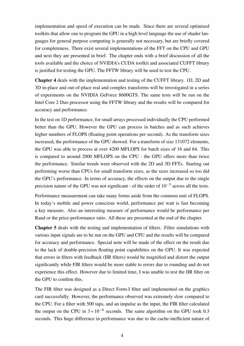
In the test on 1D performance, for small arrays processed individually the CPU performedbetter than the GPU. However the GPU can process in batches and as such achieveshigher numbers of FLOPS (floating point operations per second). As the transform sizesincreased, the performance of the GPU showed. For a transform of size 131072 elements,the GPU was able to process at over 4200 MFLOPS for batch sizes of 16 and 64. Thisis compared to around 2000 MFLOPS on the CPU - the GPU offers more than twicethe performance. Similar trends were observed with the 2D and 3D FFTs. Starting outperforming worse than CPUs for small transform sizes, as the sizes increased so too didthe GPU’s performance. In terms of accuracy, the effects on the output due to the singleprecision nature of the GPU was not significant - of the order of 10−5 across all the tests.
Performance measurement can take many forms aside from the common unit of FLOPS.In today’s mobile and power conscious world, performance per watt is fast becominga key measure. Also an interesting measure of performance would be performance perRand or the price-performance ratio. All these are presented at the end of the chapter.
Chapter 5 deals with the testing and implementation of filters. Filter simulations withvarious input signals are to be run on the GPU and CPU and the results will be comparedfor accuracy and performance. Special note will be made of the effect on the result dueto the lack of double-precision floating point capabilities on the GPU. It was expectedthat errors in filters with feedback (IIR filters) would be magnified and distort the outputsignificantly while FIR filters would be more stable to errors due to rounding and do notexperience this effect. However due to limited time, I was unable to test the IIR filter onthe GPU to confirm this.
The FIR filter was designed as a Direct Form-I filter and implemented on the graphicscard successfully. However, the performance observed was extremely slow compared tothe CPU. For a filter with 500 taps, and an impulse as the input, the FIR filter calculatedthe output on the CPU in 3 ∗ 10−6 seconds. The same algorithm on the GPU took 0.3seconds. This huge difference in performance was due to the cache-inefficient nature of
4

the algorithm implemented and every time a memory access was made there was a verylarge performance cost associated with it.
Chapter 6 concludes that GPUs can offer large performance benefits when applied to sig-nal processing tasks. However, one must be aware of the differences in the programmingmodel between the CPU and GPU. A naive implementation of an algorithm that is effi-cient on the CPU will most probably give unsatisfactory performance as was seen in thecase of the FIR filter. The main portion of the thesis concludes with my recommendationsfor further research in this field.
The Appendices contain information about the history of the GPU as well as a previewof some of the new initiatives being taken by the major players in the CPU and GPUmarket to enter the GPGPU field. Following that is some technical information about thehardware that was used in the tests. Tables of all the results obtained from the tests areincluded here as well.
5

Chapter 2
The Graphics Processor & Pipeline
In order to tackle the problem of running general-purpose programs on a specialised pro-cessor such as the GPU, one must first understand exactly how it works. All the termi-nology and programming paradigms for GPUs are aimed at making it easy to render 3Dimages on a 2D screen. In order to leverage the processing power available to the fullestextent, the data and code must be optimised for the graphics pipeline. In this section wewill examine these elements in detail.
2.1 The Graphics Processing Unit
The GPU is the actual chip on a graphics card that performs the operations required torender pixels on the screen. Modern consumer GPUs are stream processing SIMD pro-cessors. This means that they are optimised to perform a single instruction, called a kernelfunction, on each element of a large dataset at the same time.
The driving force behind the rise of the GPU has been the multibillion-dollar video gameindustry. In fact the demand for graphics power is so great that GPU performance hasbeen exceeding Moore’s law by over 2.4 times a year [2]. The reason for this dramaticincrease in power is the lack of control circuitry which occupies a majority of the spaceon a modern CPU. In contrast to this, GPUs devote almost all the space on the chip tothe Arithmetic Logic Units (ALUs) thus tremendously increasing their pure processingpower, but at the cost of severely penalising incorrect branch choices. For traditionalpurposes this is not an issue, but when attempting to use the GPU as a general purposeprocessor, this is a serious issue that must be taken into account. Figure 2.1 shows therelative amounts of transistors devoted to different tasks on the CPU as compared to theGPU.
Graphics cards are often marketed as being compliant with a specific graphics API andin that regard the industry is currently at the changeover point from the older Direct3D9.0 based cards to the new Direct3D 10 compliant ones. A number of significant changes
6
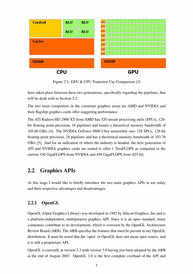
Figure 2.1: GPU & CPU Transistor Use Comparison [3]
have taken place between these two generations, specifically regarding the pipelines, thatwill be dealt with in Section 2.3.
The two main competitors in the consumer graphics arena are AMD and NVIDIA andtheir flagship graphics cards offer staggering performance.
The ATI Radeon HD 2900 XT from AMD has 320 stream processing units (SPUs), 128-bit floating point precision, 16 pipelines and boasts a theoretical memory bandwidth of105.60 GB/s [4]. The NVIDIA GeForce 8800 Ultra meanwhile uses 128 SPUs, 128-bitfloating point precision, 24 pipelines and has a theoretical memory bandwidth of 103.70GB/s [5]. And for an indication of where the industry is headed, the next generation ofATI and NVIDIA graphics cards are touted to offer 1 TeraFLOPS as compared to thecurrent 330 GigaFLOPS from NVIDIA and 450 GigaFLOPS from ATI [6].
2.2 Graphics APIs
At this stage I would like to briefly introduce the two main graphics APIs in use todayand their respective advantages and disadvantages.
2.2.1 OpenGL
OpenGL (Open Graphics Library) was developed in 1992 by Silicon Graphics, Inc and isa platform-independent, multipurpose graphics API. Since it is an open standard, manycompanies contribute to its development, which is overseen by the OpenGL ArchitectureReview Board (ARB). The ARB specifies the features that must be present in any OpenGLdistribution. It must be noted that the ’open’ in OpenGL does not mean open source, andit is still a proprietary API.
OpenGL is currently at version 2.1 with version 3.0 having just been adopted by the ARBat the end of August 2007. OpenGL 3.0 is the first complete overhaul of the API and
7

makes it completely object based, not state based. It will include new developments inthe GPU field as well as improve performance in existing technologies [7].
2.2.2 Direct3D
Direct3D is a part of the DirectX collection of APIs that provides libraries for creating 3Dimages on the Windows platform. It is a proprietary API and is developed and maintainedby Microsoft. While in its initial release Direct3D was seriously flawed and lacked manyof the functions provided by OpenGL, it has since evolved and is now at least its equal inperformance and ease of use [8].
Direct3D is now up to version 10 which is available solely on Windows Vista as part ofDirectX 10.0. Older Windows operating systems use Direct3D 9. There are several majorimprovements in Direct3D 10 that will be discussed in Section 2.3.2.
2.2.3 Comparing Direct3D and OpenGL
OpenGL and Direct3D are fundamentally different in their approaches to solving theproblem of creating 3D graphics. OpenGL aims to specify a 3D rendering system thatmay be hardware accelerated. Direct3D on the other hand is derived from the featuresthat the hardware supports [9].
This difference extends to the way they both work as well. Direct3D allows the applica-tion to manage the hardware resources, thus giving the creator more control. OpenGL onthe other hand simplifies the API for the application developer by placing the burden ofmanaging the hardware resources on the creator of the hardware driver.
The major advantage that OpenGL has over Direct3D is its platform independence. Forthis reason it is favoured by most researchers and graphic designers. However, due tothe widespread use of the Windows operating system on PCs, Direct3D has become thepreferred platform for game development which is the major driver of GPU progress.
Finally, OpenGL allows hardware vendors to create their own extensions to the standardand advertise them to the API via the driver. This allows new functionality to be exposedquickly, at the cost of some confusion when different vendors use different APIs to imple-ment similar extensions. Direct3D, being developed and maintained solely by Microsoft,is more consistent in the features offered at the cost of denying access to vendor-specificfeatures.
Thus it can be seen that the pros and cons of both of these APIs currently balance eachother out and the choice of API must come down to the specific needs of the user andtools available.
8

2.3 The Graphics Pipeline
When discussing the graphics pipeline, it is important to recognise the relationship be-tween the software, the API and the hardware. This is because the pipeline is stipulatedby the specific API in use, be it OpenGL or Direct3D. Generally the graphics API definesthe way the software interacts with the hardware and specifies certain minimum require-ments for compliance. Because of this, it is often called a Hardware Abstraction Layer(HAL) [10].
2.3.1 The Simplified Pipeline
The generic graphics pipeline shown in Figure 2.2 is the pre-Direct3D 10.0 model whichwe shall examine first. Instructions are sent from the application to the GPU. The APIhandles the transformations that occour between and including the ‘command’ and ‘frag-ment’ stages [11] and the output is finally sent to the appropriate display.
Figure 2.2: A Conceptual Pipeline [12]
I will now present an in-depth look at exactly what the the GPU does at each stage of thepipeline. The start of the pipeline is at the Application itself. It is here that the objectsto be rendered are represented as basic geometric primitives - most commonly triangles.There are some visual optimisations that take place at this stage such as occlusion cullingand visibility checking that does not play a big role in GPGPU and can be safely ignoredfor our purposes.
The Command stage buffers and interprets the application’s call and translates it into aform understandable by the hardware.
9

Now on to the Geometry stage. In practice this stage is implemented in a module calledthe Vertex Shader Unit as it acts on the vertices of the triangles sent in from the appli-cation. The Vertex Shader Unit operates on the single instruction multiple data (SIMD)principle and has multiple execution units called Vertex Pipelines to allow high through-put. This stage is very useful in GPGPU applications as here is where an image wouldusually undergo transformations and projections to render the scene from the viewpointof the virtual camera. These same transformations can be applied to any dataset andbenefit from the parallel nature of the execution. The Vertex Pipeline is controlled by aprogram called a Vertex Shader, written in a shading language. These can be low-level(Assembler) or high-level (HLSL, GLSL, Cg). In general the performance gained byusing the low-level language is offset by its complexity to learn and implement. Mostmodern graphics applications use high-level shader languages to control the execution inthe Vertex Pipelines.
The next stage in the general pipeline is the Rasterisation stage. This is done in theFragment Processing Unit. It is also called the Pixel Shader Unit. Like the Vertex ShaderUnit, it operates on the SIMD principle and has a number of Fragment or Pixel Pipelinesthat can be programmed by means of a Pixel Shader. In general, pixel pipelines aregrouped into 4 and can thus process 4 fragments at a time. These ‘quads’ are the smallestelements processed by the Pixel Shader Unit. As in the Vertex Shading Units, PixelShading Units can also be used to implement GPGPU.
The Texture stage is managed by the Texture Management Unit. They allow access to anumber of predefined textures from within the Pixel or Vertex Pipelines. They fetch theappropriate texture from the memory, transform and project it, filter it and finally make itavailable to the fragment being processed.
The final stage of the API’s pipeline is the Fragment stage. This takes place in the RasterOperation Unit, which is composed of several Raster Operation Processors or Z-pipes.The fragments that leave the Pixel Pipeline may still undergo some changes before theyare ready to be displayed. Some tests they undergo are the scissor, alpha, stencil, depthand colour blending tests. Again, none of these are specifically important to GPGPU andthus will be omitted from this discussion. The final image is now ready to be written tothe frame buffer and displayed on screen.
Figure 2.3 shows a complete graphics pipeline as it would be implemented in hardware.
10

Figure 2.3: Hardware Pipeline [11]
11
2.3.2 The New Direct3D 10 Pipeline
Now that we have sufficient understanding of the previous generation of graphics cards,let us briefly examine the major aspects of the Direct3D 10 breed. With Direct3D 10,the 3D pipeline has become completely programmable, finally moving away from fixedfunction pipelines completely [13] as shown in Figure 2.4. While it appears similar tothe older generation, and most of the stages perform similar functions, there are somesignificant differences namely the new Input Assembler, Geometry Shader and OutputMerger stages.
Figure 2.4: The Direct3D 10 Pipeline [13]
Firstly, the Input Assembler takes in the index and vertex streams and assembles theminto the geometric primitives (triangles, line lists, etc.) that will be used in other stagesof the pipeline. The secondary purpose of the Input Assembler is to make the shadersmore efficient by attaching system-generated values called ’semantics’. These semanticscan reduce processing to only those primitives, instances or vertices that have not beenprocessed yet [14]. Finally, the Input Assembler also deals with Stream-Out data, whichis fed back into the pipeline from the Geometry Shader.
The second new stage is the Geometry Shader, which allows for the execution of shader-code with multiple vertices as input and the generation of vertices as output. In additionto this, the output from the Geometry Shader can be fed back into the Input Assembler to
12

be re-processed. This allows multi-pass geometry processing with minimal interventionby the CPU which is good for parallelism.
Finally, we get to the Output Merger. This is the last stage of the pipeline and takesthe results of the previous stages, combines it with the contents of the render target andproduces the final pixel value that is displayed on the screen.
2.4 Review of Literature
2.4.1 The FFT on a GPU
Moreland and Angel have co-authored two papers dealing with the implementation ofsignal processing primitives on a GPU[15, 2]. In them, once they explain fundamentalconcepts such as the impulse response, convolution and the Fourier transform, the authorspresent the discrete Fourier transform (DFT) and the method for performing it efficientlyon a computer - the fast Fourier transform. There are several algorithms that implementit for different kinds of input data. One of the most popular methods is the Cooley-Tukeyalgorithm. This algorithm reduces the operational complexity of performing the DFT oninput transforms who’s size is a power of two from O(N2) to O(N logN). This is thealgorithm that Moreland and Angel implemented in their paper.
The algorithm works on the principle of divide and conquer. The input is split in twowith one half being all the even indices and the other, the odd indices. The Fourier trans-form may be applied separately to each half and the two halves combine to form a fulltransform. This is applied recursively to get N/2 DFTs of 2 points. In practice insteadof using recursion, the algorithm implements an iterative butterfly network. Each 2-pointDFTs requires two complex multiplications and a complex addition. These results arethen combined into the final output.
There are several optimisations to the basic algorithm to ensure that the execution is asfast as possible. One is to reverse the bits of the input indices to allow the program totreat the sub-sequences as continuous chunks in the array. Another is to use the conjugatenature of real samples to enable frequency compression.
Moreland and Angel implemented this algorithm on the graphics card by programmingthe fragment processing unit of the graphics pipeline in Cg, a shader programming lan-guage. The FFT was first applied to each row, then to each column. The results obtainedfrom their tests showed their application performing on average at about 2.5 GigaFLOPSand taking 2.7 seconds on an NVIDIA GeForce FX 5800 Ultra as compared to 0.625 sec-onds (or 2 seconds if the transforms were not padded appropriately) on a 1.7GHz IntelXeon processor using FFTW. This, the authors felt, was a competitive result, especiallygiven that the Intel Xeon cost several times as much as the GeForce FX 5800.
13

2.4.2 Designing Algorithms for Efficient Memory Access
In the paper entitled “A Memory Model for Scientific Algorithms on Graphics Processors”[16], Govindaraju et al. present a cache-efficient algorithm for implementing memoryintensive scientific applications, including the FFT, on modern GPU architectures.
The authors describe the memory model of GPUs and how it differs from the traditionalCPU memory model. In essence, GPUs consist of small write-through caches near thefragment processors and use a dedicated high-bandwidth, high-latency memory subsys-tem as shown in Figure 2.5. This is in contrast to the low-latency and low-bandwidthmemory that the CPU accesses. It is due to this high latency that the efficient use of theGPU’s cache can significantly increase the speed of some memory intensive algorithms.
Figure 2.5: GPU and CPU Memory Models[17]
In order to mask the high latency, GPUs prefetch blocks of data values from the DRAM-based video memory into small, fast SRAM-based caches that are local to the fragmentprocessors. This allows the GPU’s bandwidth when accessing the main memory to beup to 10 times that of the CPU. Also, due to their parallelism and the fact that they havefewer pipeline stages than CPUs, GPUs have much smaller caches which means that onlya few blocks can fit in the cache at a time.
When designing algorithms for the GPU, it is important to take these factors into consid-eration. For example, since GPUs are able to compute extremely fast, it is preferable toavoid copying any extra data to the GPU if it is possible to calculate it on the GPU duringexecution. Additionally, since GPUs are optimised to operate on 2D arrays, 1D arraysmust be mapped onto a 2D array for optimum efficiency.
14

Chapter 3
Tools Available for General-PurposeComputation on a GPU
Given the enormous processing power of GPUs, it is easy to see why interest in graph-ics cards as general purpose processors is on the rise. Besides the increases in raw power,graphics processors have become increasingly programmable. Graphics cards support fullIEEE-754 single-precision vectorised floating-point operations [1] and it has been possi-ble to use high-level shader languages to program the vertex and pixel pipelines sincethe release of the NVIDIA GeForce 3 and ATI Radeon 8500 [18]. More recently, withthe release of the Direct3D 10 compliant GPUs with their unified shaders and easy pro-grammability, there have been attempts to make programming for the GPU even simplerwith vendor supported APIs. This chapter will investigate some of the APIs and toolsavailable that facilitate the application of GPUs to general processing tasks followed byan overview of the libraries dealing specifically with implementing the FFT.
3.1 High Level GPGPU APIs
With the introduction of their respective Direct3D 10 cards, both AMD and NVIDIA havereleased special APIs to facilitate their application in general purpose processing. Theseare NVIDIA’s CUDA™ (Compute Unified Device Architecture) and AMD’s CTM ™(Close to Metal) standard development kits (SDKs). In addition to these official APIs,there are two other GPGPU oriented toolsets available - BrookGPU and Rapidmind. Inthis section, we will provide an overview of each of these.
15
3.1.1 CUDA
CUDA allows programmers to write code in C that will compile to run on the graphicscard, exploiting its massively parallel nature. This technology is only available to theGeForce 8 Series graphics cards and upwards in the commercial line and Quadro Pro-fessional Graphics solutions. Older cards cannot be supported because of the somewhatlimited programmability of the pipeline. It was made available to the public on bothWindows and Linux on February 16, 2007 [19].
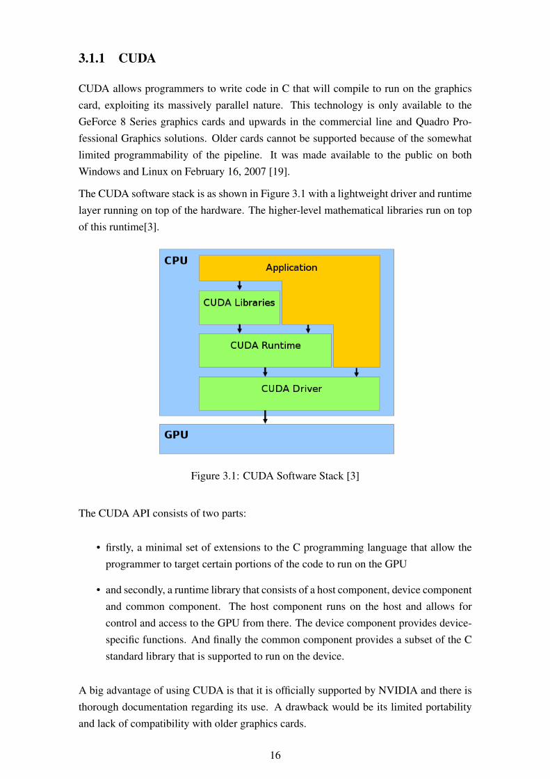
The CUDA software stack is as shown in Figure 3.1 with a lightweight driver and runtimelayer running on top of the hardware. The higher-level mathematical libraries run on topof this runtime[3].
Figure 3.1: CUDA Software Stack [3]
The CUDA API consists of two parts:
• firstly, a minimal set of extensions to the C programming language that allow theprogrammer to target certain portions of the code to run on the GPU
• and secondly, a runtime library that consists of a host component, device componentand common component. The host component runs on the host and allows forcontrol and access to the GPU from there. The device component provides device-specific functions. And finally the common component provides a subset of the Cstandard library that is supported to run on the device.
A big advantage of using CUDA is that it is officially supported by NVIDIA and there isthorough documentation regarding its use. A drawback would be its limited portabilityand lack of compatibility with older graphics cards.
16

3.1.2 CTM
AMD’s CTM is an open source project that aims to provide a thin hardware interface tothe ATI graphics cards for GPGPU [20]. It can only be used with Radeon R580 basedgraphics cards and AMD Stream Processors. It is already being used in the University ofStanford research project – Folding@Home to provide 20 to 40 times the performance ofa single CPU. Since we have discounted the use of ATI graphics cards for this study, amore detailed analysis will not be undertaken however more information is available onthe AMD website relating to CTM.
3.1.3 Rapidmind
Rapidmind is the commercial spin-off of the LibSh programming language for GPUs.It provides libraries and headers that can be used to accelerate GPGPU and is availableon both Windows and Linux. It is not limited to GPUs however and can be used toaccelerate applications on multi-core CPUs or stream processing architectures such asthe Cell Broadband Engine by IBM. Since it was born out of the free LibSh language,Rapidmind is freely available for non-commercial use.
One of the most impressive aspects of Rapidmind is its support of a wide variety of hard-ware and software. It can be used to accelerate all NVIDIA and ATI graphics cards thathave been released in the past year. It is also officially supported on Windows XP, Win-dows Vista and several of the most commonly used Linux distributions. Finally it can beused in conjunction with either the GCC 4 compiler on Linux or Microsoft Visual C++ onWindows. This portability is very important and a great advantage of using Rapidmind[21].
3.1.4 BrookGPU
Brook is a stream programming language and BrookGPU is a compiler and runtime im-plementation of Brook for graphics hardware. They are both research projects at StanfordUniversity [22]. Brook is described on its website in the following manner:
”Brook is an extension of standard ANSI C and is designed to incorporate theideas of data parallel computing and arithmetic intensity into a familiar andefficient language.”
- BrookGPU: Introduction [22]
17

3.2 Shading Languages
Apart from the high-level libraries and APIs for GPGPU, one can exploit the more directcontrol over the shaders that is offered by shading languages. These are still not as lowlevel as assembly code but offer fine-grained control over the graphics pipeline.
3.2.1 Cg
Cg is NVIDIA’s shading language and extends the C programming language to allowprogramming the vertex and pixel shaders in GPUs. Code written in Cg is portable toa wide range of platforms and hardware. It is compiled using the Cg compiler whichoptimises the code for the hardware on which it is to be run [23].
3.2.2 HLSL
HLSL (High Level Shading Language) is the proprietary language used by Microsoft’sDirect3D API. It is similar to NVIDIA’s Cg programming language [24]. In Direct3D10 there are three shaders available – vertex, pixel and geometry. Geometry shaders areabsent from previous versions.
3.2.3 GLSL
OpenGL Shading Language (GLSL or GLslang) is the C-based shader programming lan-guage that became a part of OpenGL from version 2.0. It offers direct, platform indepen-dent control of the graphics pipeline. The code written in GLSL is passed to the hardwaredriver to compile and implement, thus the GPU creator can optimize the code for theirspecific architecture [25].
3.3 Existing FFT Libraries
Currently the best and most commonly used library for implementing the FFT on CPUs isone called FFTW. On GPUs, GPUFFTW, CUFFT and libgpufft are some of the librariesthat can be used.
3.3.1 CPU Based – FFTW
FFTW is an acronym for Fastest Fourier Transform in the West. It is an optimised librarywritten in ANSI C that can compute Discrete Fourier Transforms (DFT) of data witharbitrary length, rank, multiplicity and general memory layout. It is faster than most
18

other implementations available [26]. FFTW uses a variety of algorithms and chooses thebest one based on the hardware architecture it is being run on. The library analyses thehardware and then creates a ‘plan’ that it uses to perform the rest of the computation.
Some of the algorithms used are the Cooley-Tukey algorithm, the prime factor algorithm,Rader’s algorithm for prime sizes, and a split-radix algorithm (with a variation due to DanBernstein) [27]. FFTW’s code generator also produces new algorithms on the fly whencreating the plans.
FFTW can compute:
• the DFT of both real and complex data,
• the DFT of even- or odd-symmetric real data (discrete cosine or sine transforms)
• the input data can have arbitrary length. FFTW employs O(n log n) algorithms forall lengths, including prime numbers.
3.3.2 GPU Based
Before beginning the discussion of the FFT libraries available for the GPU, it must benoted that the current generation of graphics cards from both NVIDIA and ATI are single-precision processors. Graphics cards that are capable of double-precision will be releasedat the end of this year [28]. There have also been some attempts at emulating doubleprecision.
GPUFFTW
This is a freely available library that implements the FFT in a manner that is optimisedfor graphics processors. It is related to the CPU based FFTW in name only, not in termsof its implementation. The GPUFFTW algorithm uses Stockham autosort.
It is fairly limited at the present time because it can only handle 1D power-of-two singleprecision FFTs [29]. 2D and 3D versions are in development and may become availablesoon. A sample benchmark from the official website that shows the performance increaseover CPUs is shown in Figure 3.2. It works on NVIDIA GPUs from the GeForce 6 seriesonwards.
19

Figure 3.2: GPUFFTW Benchmarks [30]
CUFFT
This is NVIDIA’s proprietary FFT implementation that only works with the newest gen-eration (GeForce 8 series) of GPUs. It is a part of the CUDA library. Some of its featuresare [31]:
• 1D, 2D, and 3D transforms of complex and real-valued data.
• Batch execution for doing multiple 1D transforms in parallel.
• 2D and 3D transform sizes in the range [2, 16384] in any dimension.
• 1D transform sizes up to 8 million elements.
• In-place and out-of-place transforms for real and complex data.
The CUFFT library uses a technique similar to that employed by the FFTW library forCPUs whereby it first creates specific plans for the dataset, architecture and transforms inuse and then implements it on the GPU.
libgpufft
This is an older library that also allows for GPU based FFT calculation on both ATIand NVIDIA hardware. It is implemented using the BrookGPU compiler and uses animproved version of Cooley-Tukey FFT algorithm. The newer GPUFFTW is as much as3 times as fast for 1D FFTs [30]. However, this library does have some advantages [32]:
20

• libgpufft has an identical communication pattern for each stage, allowing the samefragment program to be used across all stages. Consequently libgpufft does notincur the cost of switching the fragment program between stages.
• libgpufft packs two complex floating point numbers into each fragment, allowingthe 4-wide units to be used at maximum efficiency.
• libgpufft is written in Brook, making its code simple to understand and adapt.
3.4 Discussion and Comparison of the Tools for Use inThis Thesis
All the tools presented in this chapter have been used successfully to implement variousapplications on the GPU. The question now turns to which of these is most suitable forthe task at hand and which would provide the best results in the limited time available.This choice must be made based on the information gathered here as there is insufficienttime to test each tool individually.
Firstly, I have decided against implementing the FFT algorithm using low-level shadersbecause there already exist several highly optimised libraries. Secondly, CTM must beremoved from consideration due to the poor driver support for AMD graphics cards onLinux based operating systems. Now I will consider the other tools.
RapidMind and BrookGPU are both excellent tools that are being actively developed.Moreover they support a wide variety of graphics cards. RapidMind however, perhapsbecause it is a commercial product, seems to offer better documentation and support.Finally the CUDA toolkit is a proprietary API developed and maintained by NVIDIA andsupports only its latest generation of GPUs. However this hardware is nearly a year oldand widely available at a variety of price points. Given the factors discussed here, eitherCUDA or RapidMind would be good choices.
Now moving on to the FFT libraries, libgpufft is good because it supports a wide varietyof hardware and offers many features, but it is a few years old and does not take advan-tage of the enhancements provided in the new hardware. GPUFFTW is extremely fastat calculating 1D FFTs and is optimised for the latest NVIDIA hardware, but is limitedto just that. While it would be possible to implement a multidimensional FFT using adistributed single dimensional FFT, the limited time available makes that unfeasible. Fi-nally we get to NVIDIA’s CUFFT library which offers all the features required and hasexcellent documentation provided by NVIDIA.
Thus the final choice of toolkit and library that will be used for the rest of this investigationis NVIDIA’s CUDA toolkit with the associated CUFFT library.
21

Chapter 4
The FFT on the GPU
We now move on to the implementation and testing of the chosen FFT library - the CUFFTlibrary. 1D, 2D and 3D in-place and out-of-place real and complex transforms will beinvestigated.
4.1 Hardware and Environment
The hardware and operating system to be used in all the tests is shown in Table 4.1.
Type HardwareProcessor Intel Core 2 Duo E6550 Conroe 2.33GHz 4MB Unified CacheRAM Apacer 2048Mb DDR2 [DDR6400]Hard Drive Western Digital Caviar SE 160GB 7,200RPM SATA 8MB BufferVideo Card MSI NVIDIA GeForce 8600GTS 256MBPower Supply Superchannel 500W Switching Power SupplyOptical Drive LG GSA-H44N DVD WriterMotherboard MSI Intel P35 Neo-F (16x PCIe bus for GPU)
Table 4.1: Standard Test Bed
The software and drivers used are shown in Table 4.2.
Software VersionOperating System Ubuntu Linux 7.10 Beta (Gutsy Gibbon)Linux Version 2.6.22-14-genericMake Version GNU Make 3.81Compiler gcc 4.1.3X Window System X.Org 1.3.0Video Drivers NVIDIA Linux x86 100.14.11Toolkit NVIDIA CUDA v1.0FFT (CPU) FFTW 3.1.2FFT (GPU) NVIDIA CUFFT v1.0
Table 4.2: Software Environment
22
4.2 Factors affecting the FFT
Before delving into the actual tests that have been run, I will briefly explain what will betested.
4.2.1 Multi-dimensional Datasets
The dimensionality of the transform affects the execution time because, at the lowestlevel, it means that there will need to be more multiplications and additions to get theresult. Additionally the maximum transform size changes depending on the number ofdimensions due to the limited memory on the GPU.
4.2.2 Power-of-two Transforms
All transforms that are to be tested will have sizes that are integer powers of two becausecalculating the FFT is most efficient at these sizes. While it is possible to calculate theFFT of non power-of-two and prime number sized transforms, it is generally advisableto pad the input data, of size n, with zeros or employ mirroring to achieve the smallestinteger power of two greater than n [33].
4.2.3 In-place and Out-of place Transforms
An in-place FFT is calculated entirely in the original sample memory and does not requireadditional buffer memory. Out-of-place transforms however have distinct input arraysand output arrays. Out-of-place transforms are generally easier to implement and faster,however on many classes of hardware this extra space cannot be spared, hence the needfor in-place algorithms.
4.2.4 Real and Complex Transforms
There is a computational advantage when dealing with purely real signals because thenthe n point real signal can be made into an n/2 + 1 point complex signal. The FFT canthen be run on this signal and, once done, an untangling algorithm transforms the outputinto the complete FFT of the original real signal. This reduces the amount of memoryrequired to run the FFT.
23

4.3 Testing Methodology
All tests measure the performance of the GPU including the bus transfer times. Thisis because unlike when processing on the CPU, data has to be sent to the GPU to beprocessed. This means that no matter how fast the GPU is at the number-crunching, thedata transfer time will make the CPU more useful for smaller datasets as well as thosetimes when the input data changes frequently. The overhead involved in copying the datato the GPU’s memory and back also puts the burden of minimising the number of memorytransfers that take place on the application programmer.
Table C.3 in Appendix C shows the speed of memory accesses between the main memoryand the GPU cache for the test system used. This varies depending both on the GPU andthe motherboard chipset used. Having said that, I will now describe the test for both theCPU and the GPU.
On the GPU, the chosen FFT is run and the maximum number of FFTs that can be per-formed per second is counted. To ensure that there is as little influence by the operatingsystem as possible, the test is run 32 times in succession and the fastest run is recorded.The reason why the fastest run and not the average run is used is because preliminarytests showed that the variation in performance between successive runs can be very largedue to random operating system interference. Thus the averages fluctuated greatly. Toeliminate this randomness from the data the fastest run will be used. This number is thenused to calculate the performance of the FFT in MFLOPS using formula 4.1 [26].
5∗numFFT s∗nx∗ log2(nx)106 (4.1)
where nx is the transform size and numFFT s is the experimentally produced number ofFFTs performed per second.
This same procedure is followed for several other transform sizes for each type of FFTbeing considered. Errors were calculated by having the program use a specified input fileof real or complex numbers generated in Matlab. The FFT was run and the result was sentto a file. This was then compared to Matlab’s output.
On the CPU, first the fftw-wisdom command is run to create optimised plans for theCPU and chipset. Next the benchFFT benchmarking utility provided by the library isused to run the same tests that were run for the GPU. To simplify the testing, a shellscript was used to run the test 32 times and output the results to a file. Since the FFTW’sperformance was not prone to the random fluctuations caused by OS interference, theaverage of all the runs was computed. It must be noted that from the CPU usage monitorsit appears that only one core of the dual core Intel CPU was actually being used as can beseen from Figure 4.1.
24

Figure 4.1: CPU Usage for FFTW benchmark
I will only present summarised results here along with the discussion. The completeresults are tabulated in Appendix D.
4.4 Results of Tests
4.4.1 1D Transforms
The 1D transform size limit stipulated by the CUFFT library is 8 million elements. Inaddition to the test described in the last section, a feature provided by CUFFT for 1Dtransforms that is interesting to examine is the execution of the FFT in batches. Thistakes advantage of the parallelism of the GPU especially at lower transform sizes.
The graphs shown in Figures 4.2 and 4.3 are based on data captured while testing 1D inplace complex-to-complex transforms, but the trends are the same across the board forthese FFTs. The important results are:
• The performance of the CPU based FFTW algorithm, while competitive for smallersized FFTs, falls behind the GPU based implementations as the size increases.
• The GPU is very inefficient at performing single FFTs on small datasets due to thehigh overhead incurred to transfer the data to and from the GPU memory.
• As the transform size increases, the difference in performance between the batchedand single FFT methods shown in Figure 4.3 becomes very small until there isvirtually no increase in performance when applying the FFT to 262144 elements.
• The GeForce 8600GTS cannot directly compute power-of-two transforms largerthan 262144 elements due to the fact that it has only 256MB of memory on thecard. The cufftComplex datatype is 8 bytes long and when using a batch size of 64and transform size of 524288, the memory required is 524288∗64∗8 = 268435456bytes, or 256MB. Since some portion of the memory on the GPU is used by the Xwindow system, the function cannot allocate sufficient memory process the data.
25

Figure 4.2: Performance vs Transform Size for 1D FFTs
Figure 4.3: Performance vs Batch Size for 1D FFTs
26

• The 1D transform size at which the GPU FFT seems to be the most efficient is131072 elements.
• There is almost no observed difference between the performance of the in-place andout-of-place transforms. Since there is a spike at the end of the in-place plot it ispossible that the difference will begin to show for larger transform sizes but again,these cannot be tested due to the limited video memory available.
• For the out-of-place transforms shown in Figure 4.4, the difference in performancebetween the FFTW and CUFFT is only 13% for a 1024 size transform, but thatincreases until it is nearly 300% faster for transforms of size 262144.
Figure 4.4: In-Place vs Out-of-Place for 1D FFTs
4.4.2 2D Transforms
For 2D graphs the maximum transform size specified by CUFFT is 16384x16384, but intesting the program crashed for transforms larger than 1024x1024. Thus I tested trans-forms from 8x8 up to 1024x1024 in order to obtain sufficient data. As can be seen fromFigure 4.7, the effect of the high-latency memory accesses is very pronounced with lowtransform sizes but the performance increases exponentially as the size increases. At thesame time the CPU’s performance decreases roughly linearly.
There was very little difference in performance between the in-place and out-of-placeversions of the algorithm for the complex-to-complex FFT, but complex-to-real FFTsshowed a difference in performance for larger transforms.
27

Figure 4.5: Performance vs Transform Size for 2D FFTs
Figure 4.6: Increase in Performance Offered by Out-of-Place Algorithms for 2D FFTs
4.4.3 3D Transforms
3D transforms, like 2D ones, have a size limit of 16384 in all dimensions, but again thislimit could not be reached due to limited memory on the GPU. Therefore, for testing,power-of-two transform sizes from 2x2x2 to 128x128x128 were used. We observe a sim-ilar trend of performance increases to the 2D implementation. Once again, the complex-to-complex transform exhibits no performance improvement when using the in-place or
28

out-of-place algorithms.
Figure 4.7: Performance vs Transform Size for 2D FFTs
4.5 Summary of Results
Measurement 1D FFTs (64 batched) 2D FFTs 3D FFTsMinimum Performance (MFLOPS) 2821.41 36.92 1.76Maximum Performance (MFLOPS) 4935.52 6081.74 3743.42Average Performance (MFLOPS) 3899.54 2478.63 1066.11Performance per Watt1 (MFLOPS/W) 69.51 85.66 52.72Performance per Rand (MFLOPS/Rand) 2.66 3.27 2.01Sum of the Errors -1.387x10⁻⁶ 1.022x10⁻⁶ 1.519x10⁻⁵
Table 4.3: GPU FFT Performance and Accuracy Summary
Measurement 1D FFTs 2D FFTs 3D FFTsMinimum Performance (MFLOPS) 1507.39 1608.78 607.78Maximum Performance (MFLOPS) 2767.66 3466.74 3437.39Average Performance in MFLOPS 2226.51 2586.40 2222.25Performance per Watt2 (MFLOPS/W) 38.98 48.83 48.41Performance per Rand (MFLOPS/Rand) 1.80 1.87 1.85
Table 4.4: CPU FFT Performance and Accuracy Summary
29

Chapter 5
Digital Filters on the GPU
In this chapter, I will provide a brief overview of the digital filtering process and keyconcepts. Following this, I will consider the application of GPUs to simple digital filters.FIR and IIR filters will be implemented on the CPU and GPU and the performance will bemeasured. In addition, the filter output will be analysed for errors caused by the limitedprecision on the GPU.
5.1 Brief Overview of Digital Filters
I will now provide a short introduction to the topic of digital filtering with a special focuson what will be tested. For a more in-depth treatment of the topic , refer to [34] and [35].
5.1.1 Digital Filters
Filters are signal processing elements that remove unwanted parts of a signal or extractuseful parts, such as those values lying within a certain range of frequencies [36]. Digitalfilters are a class of filters that perform the task of filtering by performing numericalcalculations on sampled values of a signal.
The input analogue signal is converted into a digital one by an analogue-to-digital con-verter (ADC). The numerical operations normally involve multiplying the signals withsome constant and adding the results. The filtered signal is then converted back to an ana-logue signal by a digital-to-analogue converter (DAC). This process is shown in Figure5.1.
30
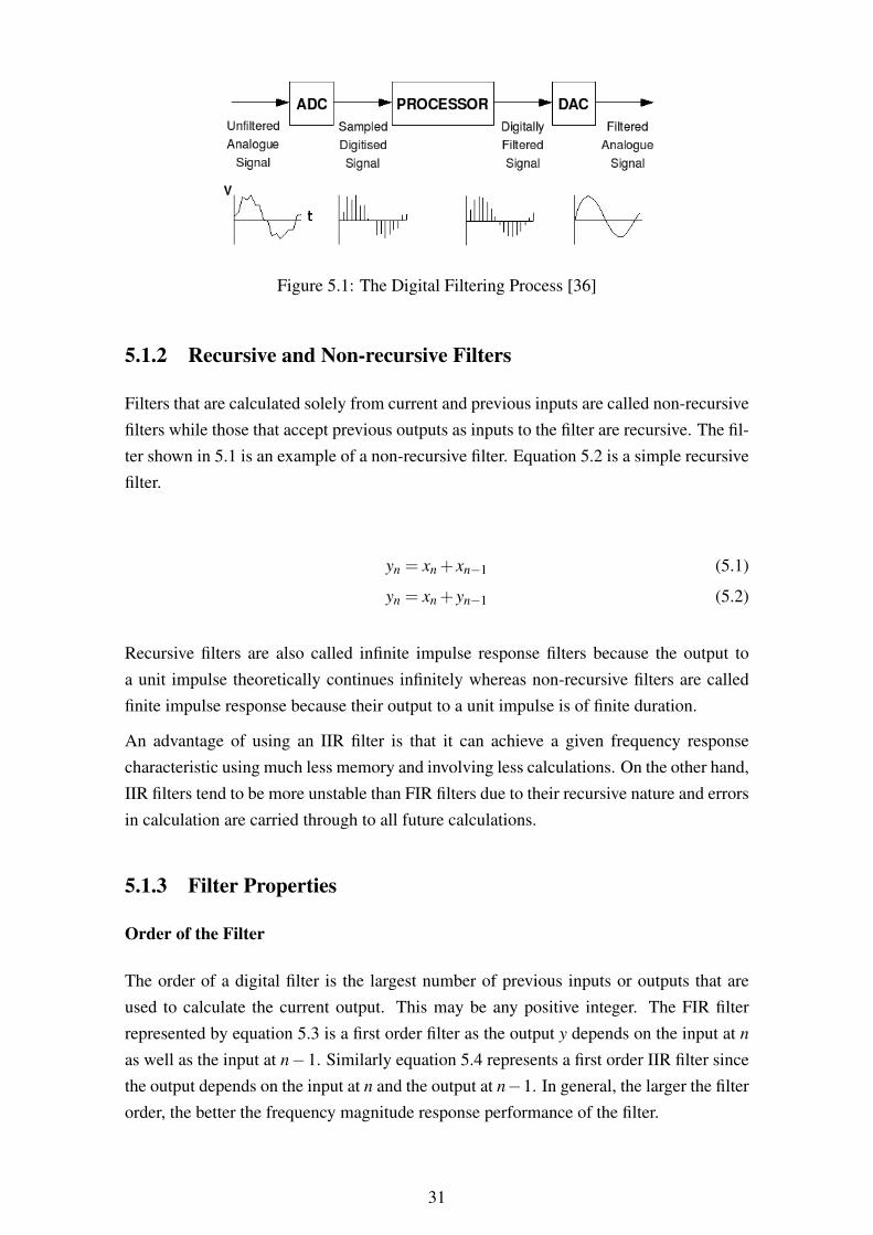
Figure 5.1: The Digital Filtering Process [36]
5.1.2 Recursive and Non-recursive Filters
Filters that are calculated solely from current and previous inputs are called non-recursivefilters while those that accept previous outputs as inputs to the filter are recursive. The fil-ter shown in 5.1 is an example of a non-recursive filter. Equation 5.2 is a simple recursivefilter.
yn = xn + xn−1 (5.1)
yn = xn + yn−1 (5.2)
Recursive filters are also called infinite impulse response filters because the output toa unit impulse theoretically continues infinitely whereas non-recursive filters are calledfinite impulse response because their output to a unit impulse is of finite duration.
An advantage of using an IIR filter is that it can achieve a given frequency responsecharacteristic using much less memory and involving less calculations. On the other hand,IIR filters tend to be more unstable than FIR filters due to their recursive nature and errorsin calculation are carried through to all future calculations.
5.1.3 Filter Properties
Order of the Filter
The order of a digital filter is the largest number of previous inputs or outputs that areused to calculate the current output. This may be any positive integer. The FIR filterrepresented by equation 5.3 is a first order filter as the output y depends on the input at n
as well as the input at n−1. Similarly equation 5.4 represents a first order IIR filter sincethe output depends on the input at n and the output at n−1. In general, the larger the filterorder, the better the frequency magnitude response performance of the filter.
31

Filter Coefficients
The first-order IIR and FIR filters can be written in the general form shown in equations5.3 and 5.4.
yn = a0xn +a1xn−1 (5.3)
b0yn +b1yn−1 = a0xn +a1xn−1 (5.4)
In filter 5.3, the constants a0 and a1are called the filter coefficients and these determine thecharacteristics of a particular filter. For example, if a0 and a1 are both 1/2, it is a two-termaverage filter. For FIR filters, the filter coefficients are the impulse response of the filter.
The general form of the IIR filter 5.4 has a symmetrical form and the coefficients aredenoted by b0 and b1.
Transfer Function
The transfer function of a digital filter allows us to describe the filter completely with acompact expression. We apply the delay operator denoted by z−1 to the symmetrical formof the filter to get the transfer function as shown in equation 5.5.
(b0 +b1z−1)yn = (a0 +a1z−1)xn
∴yn
xn=
a0 +a1z−1
b0 +b1z−1 (5.5)
The transfer function for non-recursive filters simply makes the coefficient b0 = 1 and allother b coefficients are zero. Also, for higher-order filters, there will be terms for anz−n
and bnz−n where n is the order.
32

5.2 Testing Methodology
I will be testing simple FIR and IIR time-domain filters represented by the Direct Form-Ifilter structure diagrams in Figures 5.2 and 5.3.
Figure 5.2: Direct Form-I FIR Filter Structure
Figure 5.3: Direct Form-I IIR Filter Structure
The output is tested when the input signal is:
• an impulse response
• a unit step function
• randomly generated numbers
For the tests all coefficients are set to 1. The time taken to allocate memory and set up thearrays for processing is not taken into account, only the processing time will be measured.The gettimeofday() function will be used to measure time when calculating on the CPUand cutTimer will be used on the GPU.
To measure precision, the filter output will be compared with the reference CPU imple-mentation. The difference between the two will be calculated. It is expected that thesingle precision nature of GPUs will have little effect on the output for most FIR filters.This is because errors due to rounding in one stage of the filter are not carried over to thenext stage.
IIR filters on the other hand use the output of previous stages as inputs to the next. Thishas the effect of amplifying the errors and causing the output to be inaccurate at best.
33

5.3 Finite Impulse Response Test Results
The results of testing the FIR filter are shown in the table below and the discussion fol-lows.
Number of Taps CPU Processing Time (s) GPU Processing Time (s)50 1x10⁻⁶ 1x10⁻³
100 2x10⁻⁶ 3x10⁻³
500 2x10⁻⁶ 0.4611000 4x10⁻⁶ 1.2812500 9x10⁻⁶ 7.3755000 19x10−6 32.006
10000 37x10−6 128.001
Table 5.1: Results of Performance Test
It must be stated that the implementation was not optimised for the parallel nature of theGPU As can be seen, the graphics card actually performed several orders of magnitudeworse than the CPU for the tests run. The CPU implementation offered far better perfor-mance even for a large number of taps. However, accuracy was found to be sufficient.
5.4 Infinite Impulse Response Filters
IIR filter implementation and testing could not be conducted due to time constraints. Thiswas due to the delay in hardware delivery, as it was recieved only two weeks prior to thesubmission deadline.
However the following is expected from an IIR filter implemented on the GPU:
• Increased performance on modern graphics cards due to the presence of the streamoutput which allows data in the geometry shader of the pipeline to be read out andfed back in to the input assembler to be reprocessed. IIR filters operate on similarfeedback loops and their data need not leave the processing pipeline.
• Errors due to rounding (caused by the lack of double precision floating point ca-pability) will be carried forward from previous stages. This will lead to the errorsbeing magnified as the number of filter taps increase.
34

Chapter 6
Conclusions
The main goals of this thesis as stated in Chapter 1 were to:
• Investigate the existing libraries and tools that may be used to execute signal pro-cessing primitives on a graphics card.
• Test an existing GPU-based FFT library and compare the performance and accuracyof that implementation with a reference CPU-based implementation, varying thetransform size and number of dimensions.
• Implement simple FIR and IIR filters on the GPU and compare the performanceand accuracy of the filter’s output for different input signals.
After carrying out an investigation into the nature of the GPU and the various methodsof programming it I decided to use NVIDIA’s CUDA as the tool for the second halfof my thesis. This is the actual implementation of signal processing primitives. Theimplementation and testing went smoothly for the most part except that I was unable toimplement the IIR filter due to time constraints.
6.1 Conclusions from Testing
Based on the test results of the FFT and the FIR filter, the following conclusions can bemade.
The GPU-based FFT implementation offered massive performance increases of upto 300%over the CPU for some datasets. The general trend was that the CPU was more efficientat performing single FFTs on small datasets but as the transform size or number of FFTsbeing processed at a time increased, the GPU offered better performance.
Performance per watt and per Rand was again dependent on the transform sizes. Howeverif the highest performance value obtained from testing was used as a measure of the max-imum capability, the GPU far outstrips the CPU. It offers nearly double the performanceper watt and 43% increase in performance per Rand.
35

An interesting point to note is that the performance was generally higher for 2D data. Thisis because GPUs are optimised to operate on textures, which are basically 2D arrays ofpixels. Therefore even when implementing non-graphics related algorithms on the GPU,it is best to convert the input data into one or several rectangular subsets.
The implementation of the FIR filter on the GPU was successful but offered unsatisfactoryperformance. This is due to the efficiency of the algorithm used. It was implemented usinga nested for loop over 1D data, which is computationally more efficient on the CPU thanthe GPU.
GPUs are optimised to perform a small kernel function on a large dataset in parallel andnot sequentially as in a for loop. Additionally, the algorithm did not implement the ef-ficient caching strategy discussed in Section 2.4.2 to minimise memory accesses. If thealgorithm were to be optimised properly, it would be possible to speed up the implemen-tation and make it faster than the CPU for filters with a large number of taps.
6.2 Recommendations for Further Research
In light of the findings presented above, there are several possible avenues for furtherresearch that could provide interesting and useful information or tools.
Firstly, the FIR filter that was inefficient in my implementation could be sped up with amore cache and memory aware algorithm. Another recommendation would be to applythe primitives investigated here into a larger system such as a software radio implementedon the GPU using CUDA.
One could also investigate an alternative toolkit such as RapidMind to test the FFT andfilters on and compare the performance of the two implementations.
To gain a better understanding of what it is that affects the real-world performance of thesesignal processing algorithms, tests similar to the ones used in this thesis should be run onother graphics cards. In particular AMD GPUs with their associated CTM toolkit whichis analogous to the CUDA toolkit for NVIDIA GPUs would be interesting to investigate.These GPUs have 320 stream processing units which would improve performance.
36

Appendix A
A Short History of Graphics and GPUs
The history of computer graphics can be traced back to a paper presented by Ivan Suther-land in 1963 entitled ‘Sketchpad’ at the Summer Joint Computer Conference [37]. Itallowed for interactive design on a vector graphics display with a light pen. Since thislandmark paper, graphics have come a long way through the efforts of hundreds of differ-ent people.
A.1 The 1960s
During the middle to late 1960’s, several important advances took place in the fledglingfield of graphics. A method for drawing lines and circles on a raster device was discoveredand the first computer aided design (CAD) concepts were developed. Meanwhile on thehardware side, flight simulators with real-time raster graphics were created and the firstmicroprocessor was built at Intel.
A.2 The 1970s & 1980s
The early 1970’s saw the discovery the z-buffer algorithm and texture mapping. Duringthe latter part of that decade, early games such as Pong and Pac Man became popular andcan be viewed as the starting point for the current success of graphics cards due to thegaming industry.
The 1980’s signaled the advent of the personal computer (PC) with competing modelsfrom both IBM and Apple. The first Video Graphics Array (VGA) card was also inventedand research interest in special purpose graphics processors and parallel processors wason the rise.
37
A.3 The 1990s
The 1990’s was arguably the most important decade in the brief history of computergraphics. Both the software and hardware really started to mature and became viable formass consumption. CPUs alone could no longer handle the massive amounts of data thatneeded to be processed at the necessary speeds for real-time usage, thus the standalonegraphics card was born.
Some of the highlights of the first part of the decade were the introduction of OpenGLas a standard for graphics APIs, the Reality Engine from Silicon Graphics that allowedhardware-based real-time texture mapping and the release of the Nintendo 64 game con-sole that provided real-time 3D graphics to the masses.
Towards the latter part of the 1990’s the personal computer market exploded. Compa-nies like 3dfx, ATI, Matrox and NVIDIA all jumped into the ring to claim their slice ofthe ever-expanding 3D graphics card market in both the personal and business sectors.Microsoft’s Direct3D API rose as a challenger to OpenGL on the Windows operatingsystem. Movies began to use 3D technology extensively for special effects and severalwholly 3D rendered movies were made.
On the hardware side, ever increasing clock speeds, bit widths and memory capacitiespushed the available technology to its limits. It was at this time that consumer graphicscards began using multiple pipelines to speed up processing. Graphics cards also switchedfrom using the PCI bus to the specialized AGP bus.
A.4 The 2000s
That brings us to the current decade, the 2000’s. Performance has continued to increase,doubling every year, while computer graphics have become ubiquitous. Almost all mod-ern computers have some rudimentary form of graphics processor. This has led to bettertools for creating graphics as well as giving programmers more control over the graphicspipeline. Programmable vertex, pixel and geometry shaders have opened up the GPU’spipelined architecture, giving programmers more control and the new PCI Express bushas allowed for increased parallelism when accessing the system bus.
38

Appendix B
The Future of GPGPU
We are currently at a critical juncture in the development of both CPUs and GPUs. Withthe slow convergence of these two kinds of processor, the question remains open as to thefuture of both. Is the processor of the future a massively parallel CPU a la the Cell streamprocessor from IBM that can handle GPU tasks? Or is it a GPU that can provide bettercache performance and support for branching? When we get right down to it, is therereally any difference between these two at all?
These questions will be answered in time. One thing is for sure, the era of general-purposecomputing on GPUs is just beginning. In this chapter I will provide an overview of thecurrently announced GPGPU initiatives from the major players in both the CPU and GPUarenas.
B.1 NVIDIA Tesla GPU Computing
NVIDIA has just launched a new product line in addition to their existing Quadro enter-prise line and GeForce consumer brand. They will enter the supercomputer market andoffer high performance computing (HPC) machines under the Tesla moniker [38].
These solutions will consist of graphics cards using a modified version of the G80 corethat powers the GeForce 8800 Ultra. Each of these has 128 processors in it’s computingcore, 1.5 GB of GDDR3 video memory using a 384-bit wide memory interface and iscapable of more than 500 GFLOPS of floating point performance. Initially there will bethree products in this line:
• the Tesla C870 Computing Processor is the ’entry level’ model. It costs $1,499and consists of one 8-series GPU. This graphics card uses a maximum of 170W ofpower can be connected to any PC to create a personal supercomputer.
• the Tesla D870 Deskside Supercomputer consists of two of the 8-series GPUs andattaches to a workstation via a PCI Express adapter. It uses 520W of power atmaximum load and will retail for $7,500.
39

• the Tesla S870 Computing Server is designed to fit into enterprise server clustersand consists of four of the 8-series GPUs. It scales in performance by simply addingmore of these units. It requires a maximum of 800W and costs $12,000.
This product line is aimed at more technical users such as scientists and engineers. Addi-tionally it has applications in industrial IT installations, weather prediction and graphicalvisualisation for oil and gas exploration.
A big advantage of this product line is the ability to use of the CUDA framework to easilyprogram these massively multi-threaded processors. It would be extremely difficult toeffectively hand code an optimum algorithm for more than 128 processors.
If there is a flaw in this product, however, it must be the lack of full IEEE 754 double-precision. This will limit its application to some scientific applications. However sincethe next line of consumer GPUs from NVIDIA is expected to support double-precision, itseems likely that the next range of Tesla products will include this as well.
B.2 AMD Fusion
When AMD bought ATI, the possibility of a unified CPU and GPU suddenly becamevery real. This was confirmed by AMD when they announced the AMD Fusion line ofheterogeneous multicore microprocessors. This architecture will combine GPU and theCPU into one, where those tasks that involve parallel computing will be automaticallyassigned to the GPU part of the processor and other general processing will take placeon the CPU part [39]. This will greatly simplify the programming model that applicationdevelopers have to deal with and allow them to create applications faster and easier.
A much touted aspect of this architecture is its very low thermal display power (TDP),which can be as low as 10W. This will allow these processors to be incorporated intohandheld devices as well. For GPGPU and graphics processing in general, a major ad-vantage of the Fusion architecture is faster transfer of data to and from the CPU as wellas faster memory accesses.
B.3 Intel’s “Larrabee” Project
“Larrabee” is the code name for a new many-core architecture being developed at In-tel [40, 41].The term ’many-core’ implies that the processor will have more than eightcores on one die. The existence of this architecture was just a rumour until very recently,but it has since been confirmed by several sources within Intel. There is still very littleinformation about it, however.
That said, I will briefly state what is known about this project. The Larrabee architectureis designed to be the basis of a new generation of CPUs, GPUs and HPC systems from
40
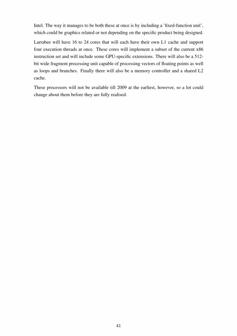
Intel. The way it manages to be both these at once is by including a ’fixed-function unit’,which could be graphics related or not depending on the specific product being designed.
Larrabee will have 16 to 24 cores that will each have their own L1 cache and supportfour execution threads at once. These cores will implement a subset of the current x86instruction set and will include some GPU-specific extensions. There will also be a 512-bit wide fragment processing unit capable of processing vectors of floating points as wellas loops and branches. Finally there will also be a memory controller and a shared L2cache.
These processors will not be available till 2009 at the earliest, however, so a lot couldchange about them before they are fully realised.
41
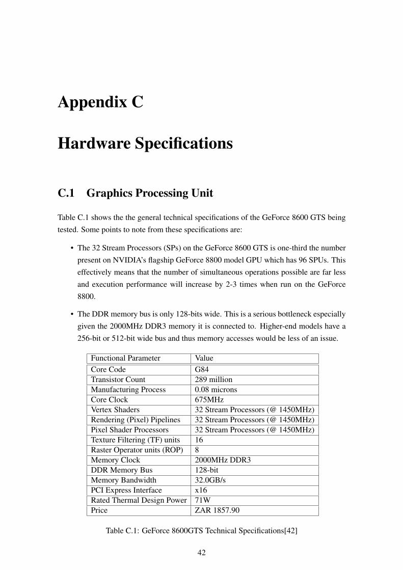
Appendix C
Hardware Specifications
C.1 Graphics Processing Unit
Table C.1 shows the the general technical specifications of the GeForce 8600 GTS beingtested. Some points to note from these specifications are:
• The 32 Stream Processors (SPs) on the GeForce 8600 GTS is one-third the numberpresent on NVIDIA’s flagship GeForce 8800 model GPU which has 96 SPUs. Thiseffectively means that the number of simultaneous operations possible are far lessand execution performance will increase by 2-3 times when run on the GeForce8800.
• The DDR memory bus is only 128-bits wide. This is a serious bottleneck especiallygiven the 2000MHz DDR3 memory it is connected to. Higher-end models have a256-bit or 512-bit wide bus and thus memory accesses would be less of an issue.
Functional Parameter ValueCore Code G84Transistor Count 289 millionManufacturing Process 0.08 micronsCore Clock 675MHzVertex Shaders 32 Stream Processors (@ 1450MHz)Rendering (Pixel) Pipelines 32 Stream Processors (@ 1450MHz)Pixel Shader Processors 32 Stream Processors (@ 1450MHz)Texture Filtering (TF) units 16Raster Operator units (ROP) 8Memory Clock 2000MHz DDR3DDR Memory Bus 128-bitMemory Bandwidth 32.0GB/sPCI Express Interface x16Rated Thermal Design Power 71WPrice ZAR 1857.90
Table C.1: GeForce 8600GTS Technical Specifications[42]
42
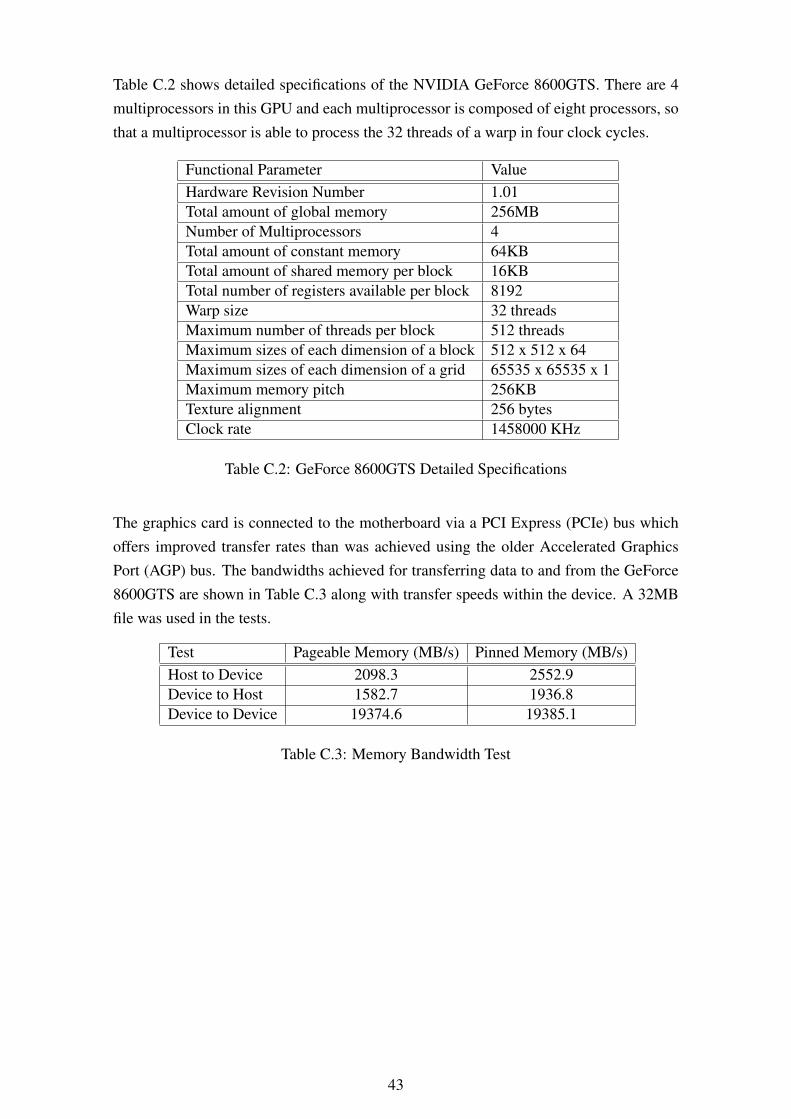
Table C.2 shows detailed specifications of the NVIDIA GeForce 8600GTS. There are 4multiprocessors in this GPU and each multiprocessor is composed of eight processors, sothat a multiprocessor is able to process the 32 threads of a warp in four clock cycles.
Functional Parameter ValueHardware Revision Number 1.01Total amount of global memory 256MBNumber of Multiprocessors 4Total amount of constant memory 64KBTotal amount of shared memory per block 16KBTotal number of registers available per block 8192Warp size 32 threadsMaximum number of threads per block 512 threadsMaximum sizes of each dimension of a block 512 x 512 x 64Maximum sizes of each dimension of a grid 65535 x 65535 x 1Maximum memory pitch 256KBTexture alignment 256 bytesClock rate 1458000 KHz
Table C.2: GeForce 8600GTS Detailed Specifications
The graphics card is connected to the motherboard via a PCI Express (PCIe) bus whichoffers improved transfer rates than was achieved using the older Accelerated GraphicsPort (AGP) bus. The bandwidths achieved for transferring data to and from the GeForce8600GTS are shown in Table C.3 along with transfer speeds within the device. A 32MBfile was used in the tests.
Test Pageable Memory (MB/s) Pinned Memory (MB/s)Host to Device 2098.3 2552.9Device to Host 1582.7 1936.8Device to Device 19374.6 19385.1
Table C.3: Memory Bandwidth Test
43

C.2 Central Processing Unit
Table C.4 shows the specifications of the Intel Core 2 Duo processor that the GeForce8600GTS will be tested against.
Functional Parameter ValueCPU core ConroeCPU socket Socket 775Clock frequency 2.33 GHzFrontside Bus Speed 1333 MHzL2 cache 4096 KBCores 2MMX/SSE/SSE2/SSE3 YesFabrication process 65 nmTDP (Max. power) 65 WCore Voltage 0.85V – 1.5VPrice ZAR 1537.80
Table C.4: Intel Core 2 Duo E6550 Specifications[43]
44

Appendix D
FFT Test Results
Here are the detailed results of the tests run for computing the FFT. All tests were doneusing pinned memory as that was faster than pageable memory (see Table C.3). Theresults are all in MFLOPS (millions of FLOPS).
D.1 1D Transforms
D.1.1 Complex-to-Complex
Transform Size Single Batch (4) Batch (16) Batch (64) CPU (FFTW)1024 752.90 1988.30 2795.88 3144.70 2587.452048 1161.21 2187.13 2627.10 2821.41 2387.644096 1861.63 2553.20 2857.45 3263.20 2401.058192 2324.81 2824.81 3074.54 3567.08 2250.3816384 2697.46 2874.08 3095.43 3282.37 2149.2132768 3047.42 3133.44 3482.42 3597.93 2101.5265536 3486.52 3780.12 4021.29 4105.18 2121.19131072 3643.15 4088.79 4222.48 4278.19 2002.24262144 3208.64 3373.79 3420.98 3444.57 1774.86
Table D.1: Performance of 1D Complex-to-Complex In-Place FFTs in MFLOPS
45
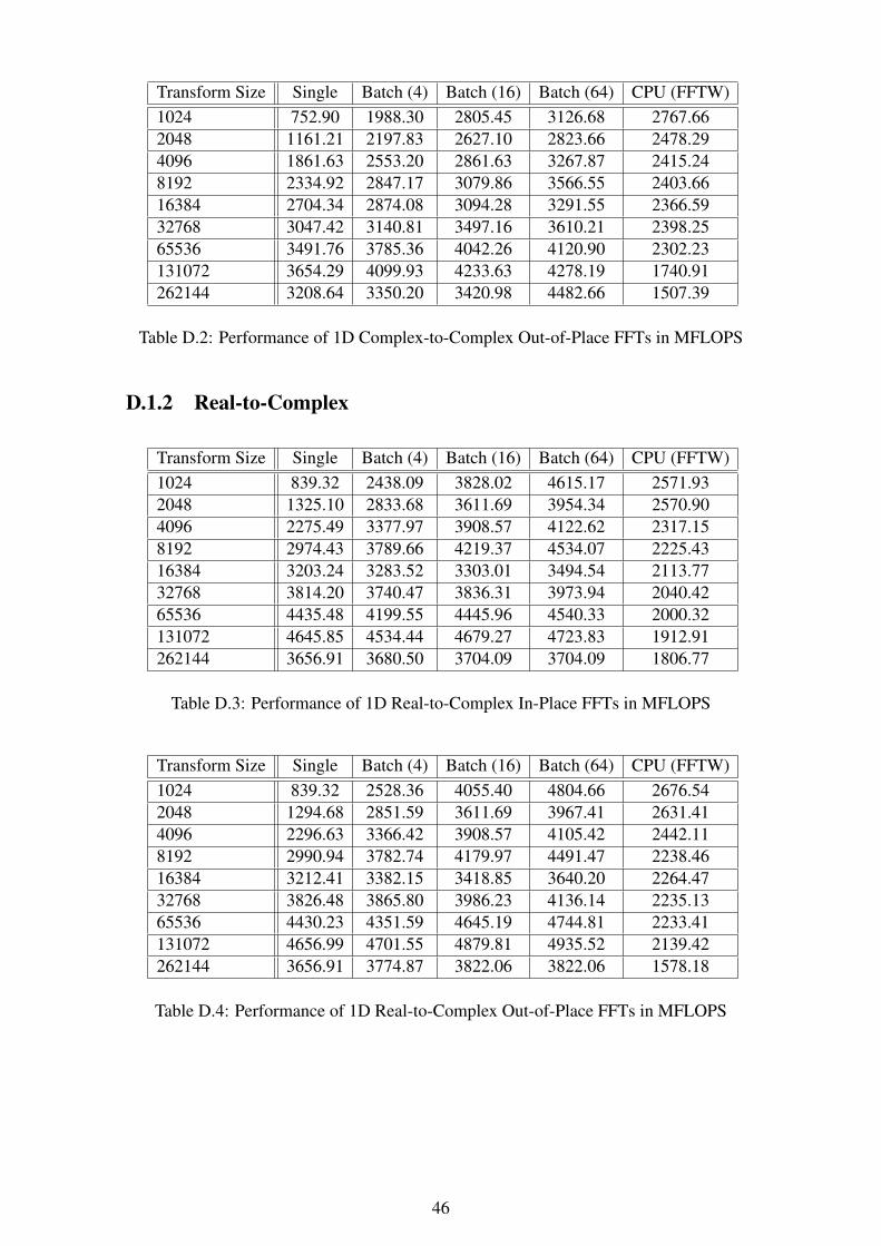
Transform Size Single Batch (4) Batch (16) Batch (64) CPU (FFTW)1024 752.90 1988.30 2805.45 3126.68 2767.662048 1161.21 2197.83 2627.10 2823.66 2478.294096 1861.63 2553.20 2861.63 3267.87 2415.248192 2334.92 2847.17 3079.86 3566.55 2403.6616384 2704.34 2874.08 3094.28 3291.55 2366.5932768 3047.42 3140.81 3497.16 3610.21 2398.2565536 3491.76 3785.36 4042.26 4120.90 2302.23131072 3654.29 4099.93 4233.63 4278.19 1740.91262144 3208.64 3350.20 3420.98 4482.66 1507.39
Table D.2: Performance of 1D Complex-to-Complex Out-of-Place FFTs in MFLOPS
D.1.2 Real-to-Complex
Transform Size Single Batch (4) Batch (16) Batch (64) CPU (FFTW)1024 839.32 2438.09 3828.02 4615.17 2571.932048 1325.10 2833.68 3611.69 3954.34 2570.904096 2275.49 3377.97 3908.57 4122.62 2317.158192 2974.43 3789.66 4219.37 4534.07 2225.4316384 3203.24 3283.52 3303.01 3494.54 2113.7732768 3814.20 3740.47 3836.31 3973.94 2040.4265536 4435.48 4199.55 4445.96 4540.33 2000.32131072 4645.85 4534.44 4679.27 4723.83 1912.91262144 3656.91 3680.50 3704.09 3704.09 1806.77
Table D.3: Performance of 1D Real-to-Complex In-Place FFTs in MFLOPS
Transform Size Single Batch (4) Batch (16) Batch (64) CPU (FFTW)1024 839.32 2528.36 4055.40 4804.66 2676.542048 1294.68 2851.59 3611.69 3967.41 2631.414096 2296.63 3366.42 3908.57 4105.42 2442.118192 2990.94 3782.74 4179.97 4491.47 2238.4616384 3212.41 3382.15 3418.85 3640.20 2264.4732768 3826.48 3865.80 3986.23 4136.14 2235.1365536 4430.23 4351.59 4645.19 4744.81 2233.41131072 4656.99 4701.55 4879.81 4935.52 2139.42262144 3656.91 3774.87 3822.06 3822.06 1578.18
Table D.4: Performance of 1D Real-to-Complex Out-of-Place FFTs in MFLOPS
46

D.1.3 Transform Times
Transform Size Complex-to-Complex Real-to-Complex CPU1024 0.03 0.03 0.0192048 0.05 0.05 0.0484096 0.06 0.06 0.1018192 0.11 0.11 0.23716384 0.22 0.24 0.53732768 0.42 0.44 1.1765536 0.76 0.83 2.46131072 1.59 1.71 5.54262144 4.92 5.15 13.17
Table D.5: Time in Milliseconds to Compute a 2D FFT (Excluding Memory Access)
D.2 2D Transforms
D.2.1 Complex-to-Complex
Transform Size GPU (In-Place) CPU (In-Place)8x8 36.92 3466.7416x16 134.73 2919.3632x32 562.64 3391.6364x64 1526.42 2633.85128x128 2729.57 2102.11256x256 3822.06 2223.84512x512 3987.21 2086.841024x1024 5138.02 1608.78
GPU (Out-of-Place) CPU (Out-of-Place)36.92 3415.6
136.53 3279.5562.64 3289.431526.42 2547.592729.57 2255.153837.79 2336.253987.21 1707.135138.02 1546.75
Table D.6: Performance of 2D Complex-to-Complex In-Place and Out-of-Place FFTs inMFLOPS
D.2.2 Complex-to-Real
Transform Size GPU (In-Place) CPU (In-Place)8x8 36.92 2587.5116x16 179.64 3086.3832x32 752.90 3340.2164x64 1683.21 2943.23128x128 3229.61 2570.5256x256 4445.96 2412.28512x512 5025.30 2113.661024x1024 5662.31 1895.41
GPU (Out-of-Place) CPU (Out-of-Place)36.92 2517.04
179.64 3257.38764.16 32591730.64 2939.333304.16 2515.514503.63 2342.785119.67 1994.536081.74 1795.26
Table D.7: Performance of 2D Complex-to-Real In-Place and Out-of-Place FFTs inMFLOPS
47

D.2.3 Transform Times
Transform Size Complex-to-Complex Real-to-Complex CPU8x8 0.03 0.03 863x10−6
16x16 0.05 0.03 0.00332x32 0.05 0.03 0.01564x64 0.09 0.07 0.102128x128 0.21 0.14 0.530256x256 0.62 0.43 2.34512x512 3.32 2.10 11.071024x1024 11.41 9.32 63.52
Table D.8: Time in Milliseconds to Compute a 2D FFT (Excluding Memory Access)
D.3 3D Transforms
D.3.1 Complex-to-Complex
Transform Size GPU (In-Place) CPU (In-Place)2x2x2 1.76 607.784x4x4 22.07 2088.888x8x8 174.53 3303.8516x16x16 249.20 2890.832x32x32 983.04 2857.3164x64x64 2288.52 2207.45128x128x128 3743.42 1646.59256x256x256 - 1741.01
GPU (Out-of-Place) CPU (Out-of-Place)1.76 653.08
21.82 2153.23173.21 3437.39248.71 2824.08985.50 2834.682288.52 1950.733743.42 1655.61
- 1797.88
Table D.9: Performance of 3D Complex-to-Complex In-Place and Out-of-Place FFTs inMFLOPS
D.3.2 Transform Times
Transform Size In-Place (C2C) Out-of-Place (C2C) CPU2x2x2 0.04 0.04 187x10−6
4x4x4 0.06 0.06 813x10−6
8x8x8 0.10 0.10 0.00716x16x16 0.93 0.93 0.09432x32x32 2.11 2.11 0.86864x64x64 7.71 7.73 10.53128x128x128 41.17 41.19 140.93
Table D.10: Time in Milliseconds to Compute a 3D FFT (Excluding Memory Access)
48
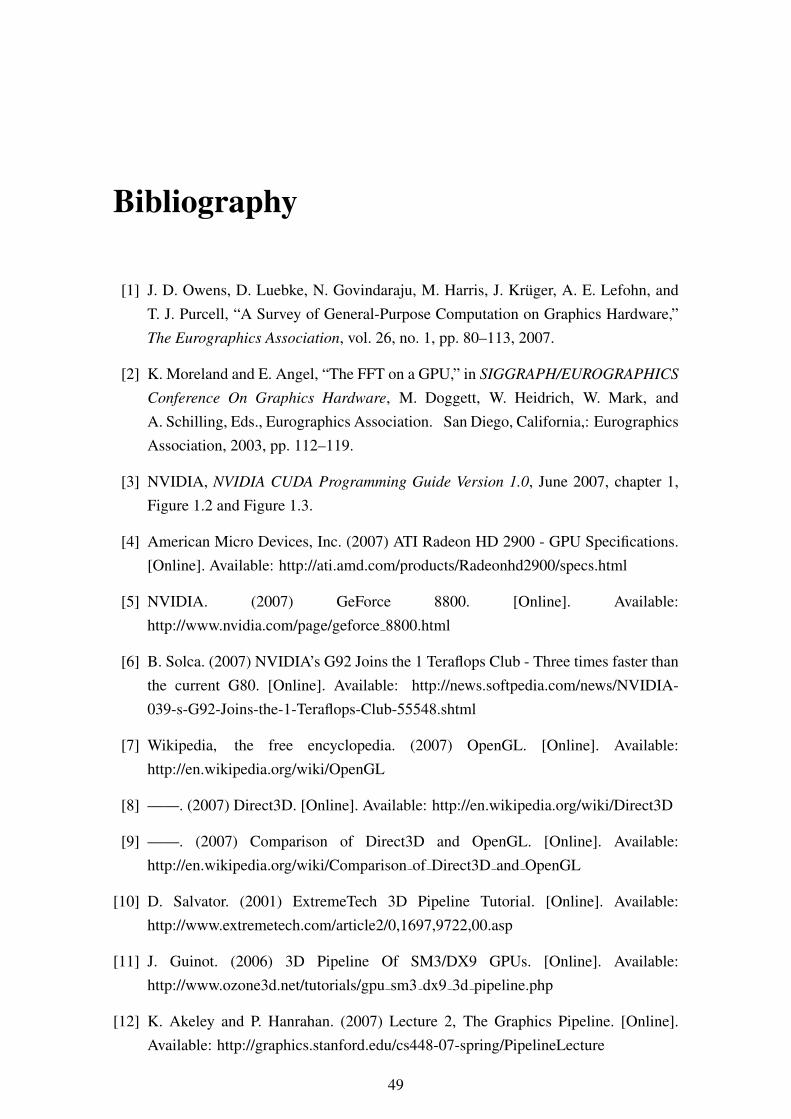
Bibliography
[1] J. D. Owens, D. Luebke, N. Govindaraju, M. Harris, J. Kruger, A. E. Lefohn, andT. J. Purcell, “A Survey of General-Purpose Computation on Graphics Hardware,”The Eurographics Association, vol. 26, no. 1, pp. 80–113, 2007.
[2] K. Moreland and E. Angel, “The FFT on a GPU,” in SIGGRAPH/EUROGRAPHICS
Conference On Graphics Hardware, M. Doggett, W. Heidrich, W. Mark, andA. Schilling, Eds., Eurographics Association. San Diego, California,: EurographicsAssociation, 2003, pp. 112–119.
[3] NVIDIA, NVIDIA CUDA Programming Guide Version 1.0, June 2007, chapter 1,Figure 1.2 and Figure 1.3.
[4] American Micro Devices, Inc. (2007) ATI Radeon HD 2900 - GPU Specifications.[Online]. Available: http://ati.amd.com/products/Radeonhd2900/specs.html
[5] NVIDIA. (2007) GeForce 8800. [Online]. Available:http://www.nvidia.com/page/geforce 8800.html
[6] B. Solca. (2007) NVIDIA’s G92 Joins the 1 Teraflops Club - Three times faster thanthe current G80. [Online]. Available: http://news.softpedia.com/news/NVIDIA-039-s-G92-Joins-the-1-Teraflops-Club-55548.shtml
[7] Wikipedia, the free encyclopedia. (2007) OpenGL. [Online]. Available:http://en.wikipedia.org/wiki/OpenGL
[8] ——. (2007) Direct3D. [Online]. Available: http://en.wikipedia.org/wiki/Direct3D
[9] ——. (2007) Comparison of Direct3D and OpenGL. [Online]. Available:http://en.wikipedia.org/wiki/Comparison of Direct3D and OpenGL
[10] D. Salvator. (2001) ExtremeTech 3D Pipeline Tutorial. [Online]. Available:http://www.extremetech.com/article2/0,1697,9722,00.asp
[11] J. Guinot. (2006) 3D Pipeline Of SM3/DX9 GPUs. [Online]. Available:http://www.ozone3d.net/tutorials/gpu sm3 dx9 3d pipeline.php
[12] K. Akeley and P. Hanrahan. (2007) Lecture 2, The Graphics Pipeline. [Online].Available: http://graphics.stanford.edu/cs448-07-spring/PipelineLecture
49
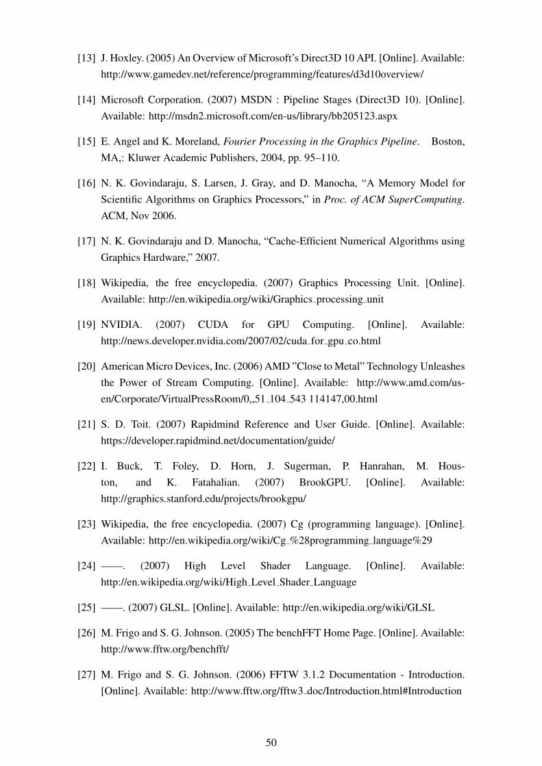
[13] J. Hoxley. (2005) An Overview of Microsoft’s Direct3D 10 API. [Online]. Available:http://www.gamedev.net/reference/programming/features/d3d10overview/
[14] Microsoft Corporation. (2007) MSDN : Pipeline Stages (Direct3D 10). [Online].Available: http://msdn2.microsoft.com/en-us/library/bb205123.aspx
[15] E. Angel and K. Moreland, Fourier Processing in the Graphics Pipeline. Boston,MA,: Kluwer Academic Publishers, 2004, pp. 95–110.
[16] N. K. Govindaraju, S. Larsen, J. Gray, and D. Manocha, “A Memory Model forScientific Algorithms on Graphics Processors,” in Proc. of ACM SuperComputing.ACM, Nov 2006.
[17] N. K. Govindaraju and D. Manocha, “Cache-Efficient Numerical Algorithms usingGraphics Hardware,” 2007.
[18] Wikipedia, the free encyclopedia. (2007) Graphics Processing Unit. [Online].Available: http://en.wikipedia.org/wiki/Graphics processing unit
[19] NVIDIA. (2007) CUDA for GPU Computing. [Online]. Available:http://news.developer.nvidia.com/2007/02/cuda for gpu co.html
[20] American Micro Devices, Inc. (2006) AMD ”Close to Metal” Technology Unleashesthe Power of Stream Computing. [Online]. Available: http://www.amd.com/us-en/Corporate/VirtualPressRoom/0,,51 104 543 114147,00.html
[21] S. D. Toit. (2007) Rapidmind Reference and User Guide. [Online]. Available:https://developer.rapidmind.net/documentation/guide/
[22] I. Buck, T. Foley, D. Horn, J. Sugerman, P. Hanrahan, M. Hous-ton, and K. Fatahalian. (2007) BrookGPU. [Online]. Available:http://graphics.stanford.edu/projects/brookgpu/
[23] Wikipedia, the free encyclopedia. (2007) Cg (programming language). [Online].Available: http://en.wikipedia.org/wiki/Cg %28programming language%29
[24] ——. (2007) High Level Shader Language. [Online]. Available:http://en.wikipedia.org/wiki/High Level Shader Language
[25] ——. (2007) GLSL. [Online]. Available: http://en.wikipedia.org/wiki/GLSL
[26] M. Frigo and S. G. Johnson. (2005) The benchFFT Home Page. [Online]. Available:http://www.fftw.org/benchfft/
[27] M. Frigo and S. G. Johnson. (2006) FFTW 3.1.2 Documentation - Introduction.[Online]. Available: http://www.fftw.org/fftw3 doc/Introduction.html#Introduction
50

[28] Wikipedia, the free encyclopedia. GPGPU. [Online]. Available:http://en.wikipedia.org/wiki/GPGPU
[29] N. K. Govindaraju and D. Manocha. (2007) GPUFFTW - Home. [Online].Available: http://gamma.cs.unc.edu/GPUFFTW/
[30] ——. (2007) GPUFFTW - Benchmarks. [Online]. Available:http://gamma.cs.unc.edu/GPUFFTW/results.html
[31] NVIDIA, NVIDIA CUFFT Library 1.0, June 2007.
[32] J. D. Owens, S. Sengupta, and D. Horn. (2005) Assessmentof Graphic Processing Units (GPUs) for Department of Defense(DoD) Digital Signal Processing (DSP) Applications. [Online]. Available:http://www.ece.ucdavis.edu/cerl/techreports/2005-3/
[33] T. H. Cormen, C. E. Leiserson, R. L. Rivest, and C. Stein, Polynomials and the FFT.Cambridge, Massachusetts,: The MIT Press, 2001, pp. 822–848.
[34] L. R. Rabiner and B. Gold, Theory and application of digital signal processing.Englewood Cliffs, N.J., Prentice-Hall, Inc.,, 1975.
[35] A. V. Oppenheim and R. W. Schafer, Digital Signal Processing. Englewood Cliffs,NJ: Prentice-Hall, 1975.
[36] dsptutor. (2007) Digital Filters: An Introduction. [Online]. Available:http://www.dsptutor.freeuk.com/dfilt1.htm
[37] W. Shoaff. (2000) A Short History of Computer Graphics. [Online]. Available:http://cs.fit.edu/ wds/classes/graphics/History/history/history.html
[38] NVIDIA. (2007) GPU Computing Solutions for HPC. [Online]. Available:http://www.nvidia.com/object/tesla computing solutions.html
[39] Wikipedia. (2007) AMD Fusion. [Online]. Available:http://en.wikipedia.org/wiki/AMD Fusion
[40] Jon Stokes. (2007) Clearing up the confusion over Intel’s Larrabee. [On-line]. Available: http://arstechnica.com/articles/paedia/hardware/clearing-up-the-confusion-over-intels-larrabee.ars
[41] ——. (2007) Clearing up the confusion over Intel’s Larrabee, part II.[Online]. Available: http://arstechnica.com/news.ars/post/20070604-clearing-up-the-confusion-over-intels-larrabee-part-ii.html
[42] Vincent Chang. (2007) NVIDIA GeForce 8600 GTS: The Full Review! [Online].Available: http://www.hardwarezone.com/articles/view.php?cid=3&id=2237
51

[43] hardware.info. (2007) Intel Core 2 Duo E6550.[Online]. Available: http://www.hardware.info/en-US/productdb/bGRkZZiWmJTK/viewproduct/Intel Core 2 Duo E6550/
[44] D. Manocha and A. Sud. (2007) COMP 790-058: GPGP: Gen-eral Purpose Computation using Graphics Processors. [Online]. Available:http://gamma.cs.unc.edu/GPGP/
[45] T. Monk. 7 Years of Graphics. [Online]. Available:http://accelenation.com/?ac.id.123.1
[46] J. Owens, “GPU Architecture Overview,” in Proc. of SIGGRAPH 2007. SIG-GRAPH 2007, 2007.
[47] Wikipedia, the free encyclopedia. (2007) Graphics Pipeline. [Online]. Available:http://en.wikipedia.org/wiki/Graphics pipeline
[48] ——. (2007) Stream Processing. [Online]. Available:http://en.wikipedia.org/wiki/Stream processing
[49] cclark and mfatica and cmorrison. (2007) CUFFT BENCHMARKING TOOL v1.0.[Online]. Available: http://forums.nvidia.com/index.php?showtopic=42482
52