signal processing and time -series analysis
TRANSCRIPT
1
1
Signal Processing and TimeSignal Processing and Time--Series AnalysisSeries Analysis
1. Signal ProcessingA. Analytical Signals are recorded as:
Spectra, chromatograms, voltammograms or titration curves(monitored in frequency, wavelength, time)
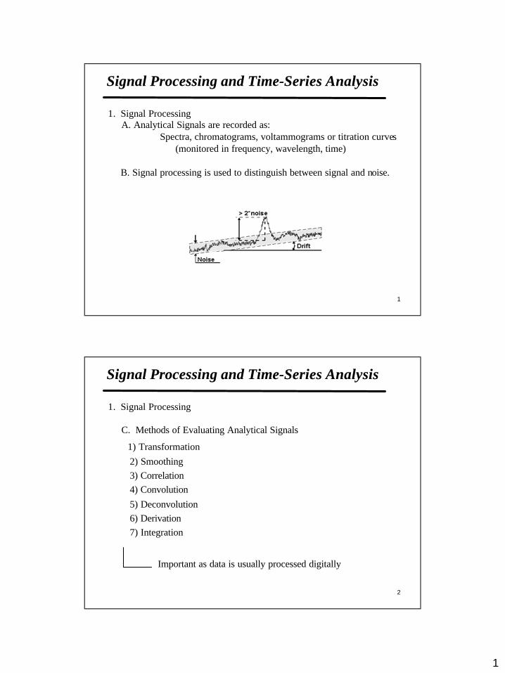
B. Signal processing is used to distinguish between signal and noise.
2
Signal Processing and TimeSignal Processing and Time--Series AnalysisSeries Analysis
1. Signal Processing
C. Methods of Evaluating Analytical Signals
1) Transformation2) Smoothing3) Correlation4) Convolution5) Deconvolution6) Derivation7) Integration
Important as data is usually processed digitally
2
3
Signal Processing and TimeSignal Processing and Time--Series AnalysisSeries Analysis
D. Digital smoothing and Filtering
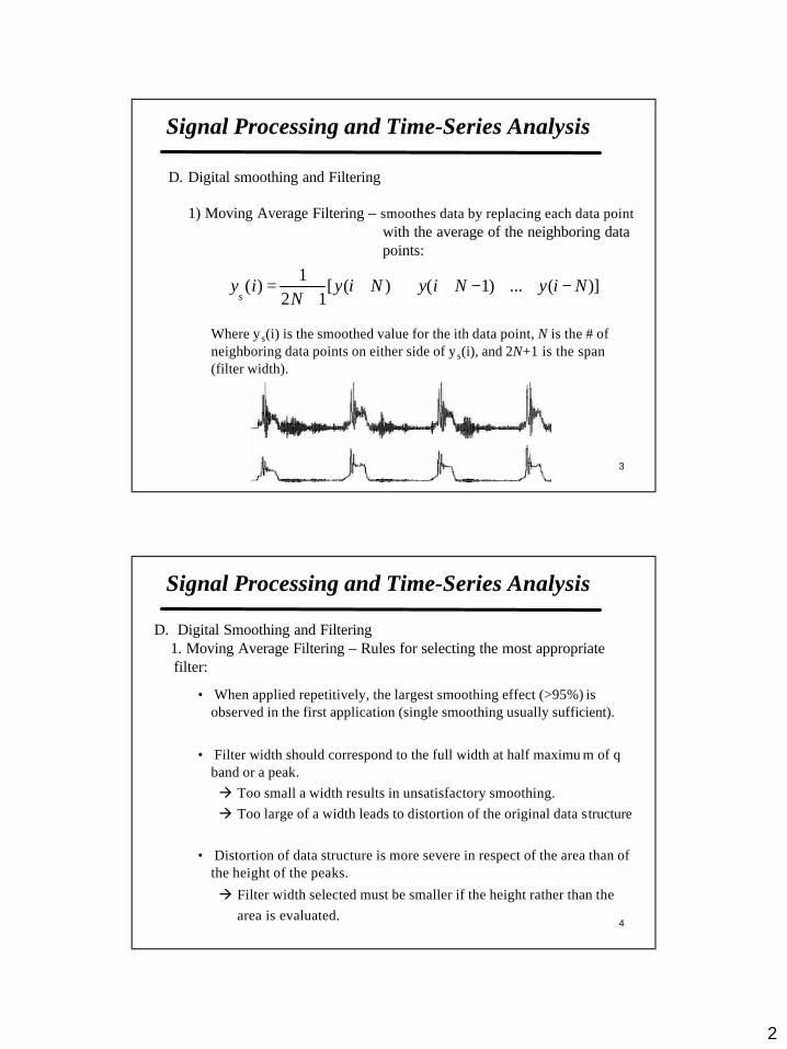
1) Moving Average Filtering – smoothes data by replacing each data point with the average of the neighboring data points:
Where y s(i) is the smoothed value for the ith data point, N is the # of neighboring data points on either side of y s(i), and 2N+1 is the span (filter width).
)](...)1()([12
1)( NiyNiyNiy
Niy
s−++−++++
+=
4
Signal Processing and TimeSignal Processing and Time--Series AnalysisSeries Analysis
D. Digital Smoothing and Filtering1. Moving Average Filtering – Rules for selecting the most appropriate filter:
• When applied repetitively, the largest smoothing effect (>95%) is observed in the first application (single smoothing usually sufficient).
• Filter width should correspond to the full width at half maximu m of q band or a peak. à Too small a width results in unsatisfactory smoothing.à Too large of a width leads to distortion of the original data structure
• Distortion of data structure is more severe in respect of the area than of the height of the peaks.
à Filter width selected must be smaller if the height rather than the area is evaluated.
3
5
Signal Processing and TimeSignal Processing and Time--Series AnalysisSeries Analysis
D. Digital Smoothing and Filtering1. Moving Average Filtering
Note: The influence of the filter-width on the distortion of the peaks can be quantified by means of the relative filter width, brelative:
5.0
bb
b filter
relative=
Where bfilter is the filter width, and b0.5 is the full width at half maximum.
6
Signal Processing and TimeSignal Processing and Time--Series AnalysisSeries Analysis
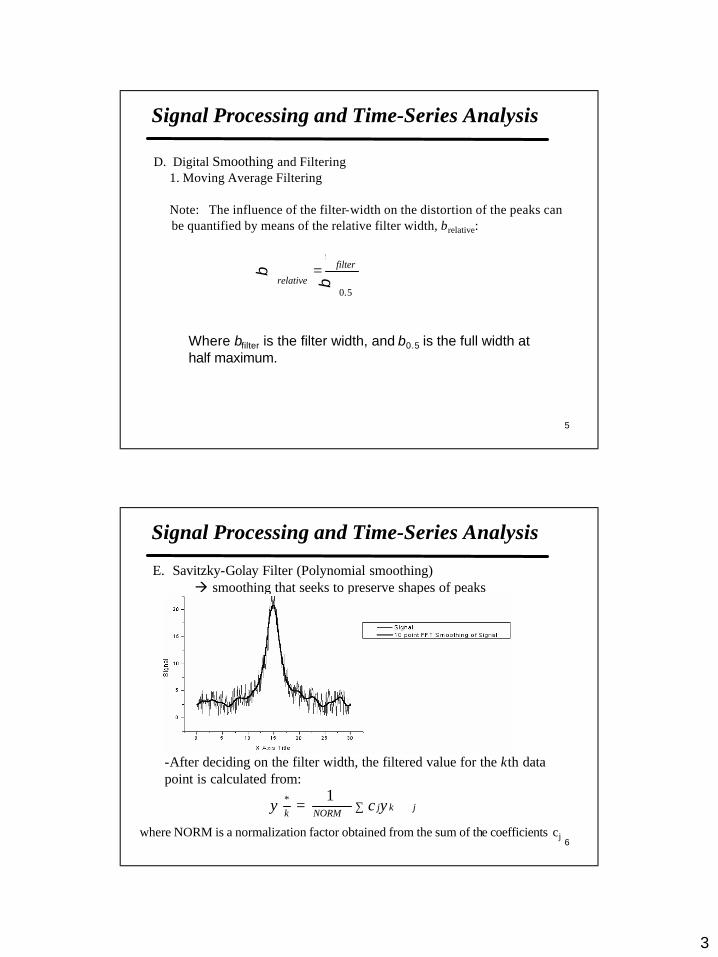
E. Savitzky-Golay Filter (Polynomial smoothing)à smoothing that seeks to preserve shapes of peaks
-After deciding on the filter width, the filtered value for the kth data point is calculated from:
where NORM is a normalization factor obtained from the sum of the coefficients cj
∑ += jkjNORMk ycy1*
4
7
Signal Processing and TimeSignal Processing and Time--Series AnalysisSeries AnalysisSignal Processing and TimeSignal Processing and Time--Series AnalysisSeries Analysis
F. Kalman Filterà Estimate the state of a system from measuring which contain random errorsà Based on two models:
1) Dynamic System model (Process)
2) Measurement Modely(k) = HT(k) x (h) + v(h)
- where x = state vector, y = the measurement, F = system transition matrix and H = the measurement vector (matrix).
- w = signal noise vector, v = measurement noise vector
- h = denotes the actual measurement or time
)1()1()( −+−= kwkxkx F
8
Signal Processing and TimeSignal Processing and Time--Series AnalysisSeries AnalysisSignal Processing and TimeSignal Processing and Time--Series AnalysisSeries Analysis
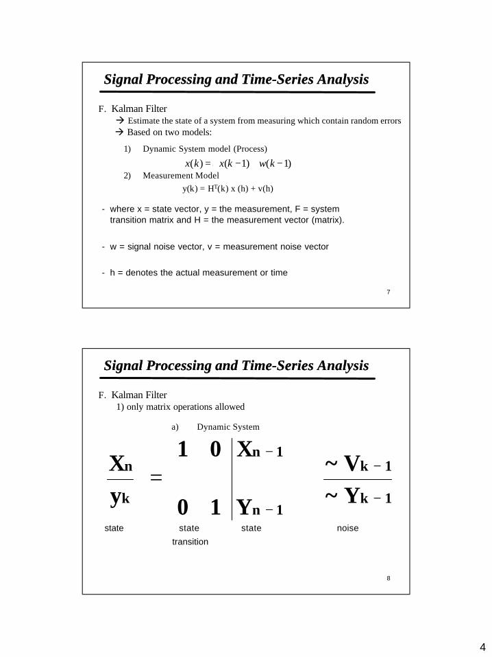
F. Kalman Filter1) only matrix operations allowed
a) Dynamic System
state state state noise
transition
+
=
−
−
−
−
1k
1k
1n
1n
k
n
Y~V~
Y
X
10
01
yX
5
9
Signal Processing and TimeSignal Processing and Time--Series AnalysisSeries AnalysisSignal Processing and TimeSignal Processing and Time--Series AnalysisSeries Analysis
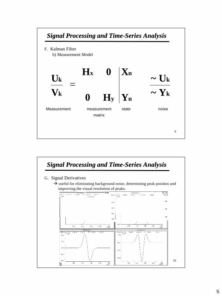
F. Kalman Filterb) Measurement Model
Measurement measurement state noise
matrix
+
=
k
k
n
n
y
x
k
k
Y~U~
Y
X
H0
0H
VU
10
Signal Processing and TimeSignal Processing and Time--Series AnalysisSeries AnalysisSignal Processing and TimeSignal Processing and Time--Series AnalysisSeries Analysis
G. Signal Derivativesà useful for eliminating background noise, determining peak position and
improving the visual resolution of peaks.
6
11
Signal Processing and TimeSignal Processing and Time--Series AnalysisSeries AnalysisSignal Processing and TimeSignal Processing and Time--Series AnalysisSeries Analysis
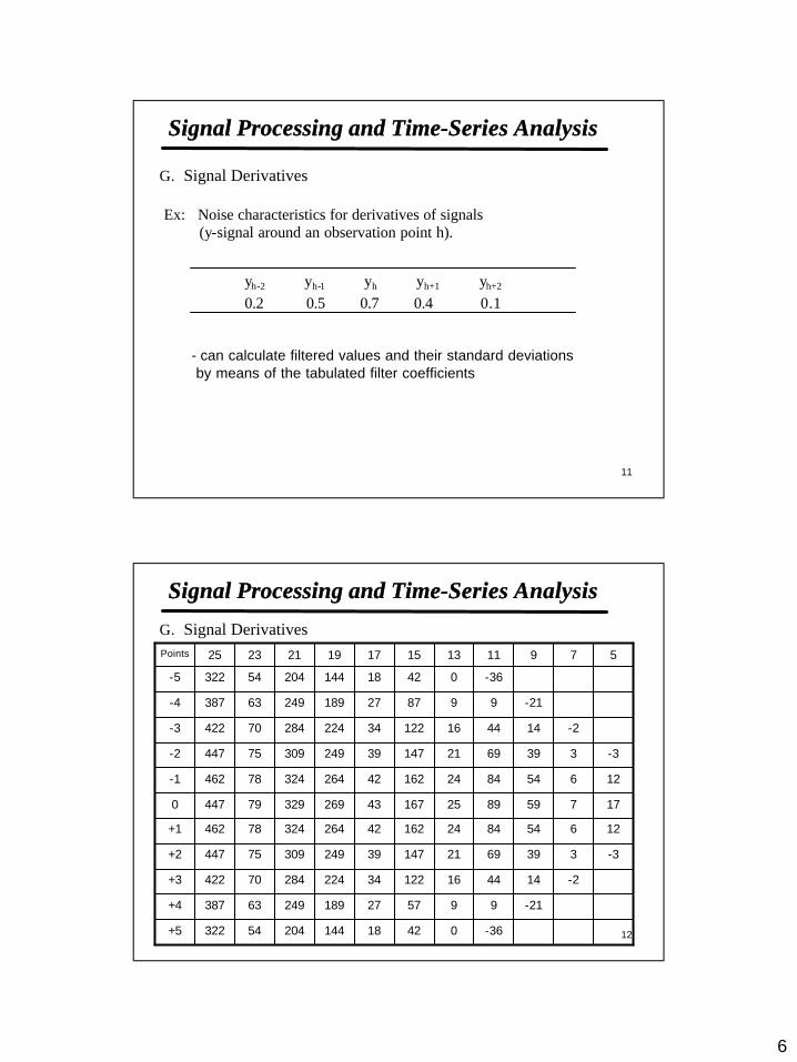
G. Signal Derivatives
Ex: Noise characteristics for derivatives of signals (y-signal around an observation point h).
yh-2 yh-1 yh yh+1 yh+2
0.2 0.5 0.7 0.4 0.1
- can calculate filtered values and their standard deviations by means of the tabulated filter coefficients
12
Signal Processing and TimeSignal Processing and Time--Series AnalysisSeries AnalysisSignal Processing and TimeSignal Processing and Time--Series AnalysisSeries Analysis
G. Signal Derivatives
-360421814420454322+5
-2199572718924963387+4
-21444161223422428470422+3
-333969211473924930975447+2
1265484241624226432478462+1
17759892516743269329794470
1265484241624226432478462-1
-333969211473924930975447-2
-21444161223422428470422-3
-2199872718924963387-4
-360421814420454322-5
5791113151719212325Points
7
13
Signal Processing and TimeSignal Processing and Time--Series AnalysisSeries AnalysisSignal Processing and TimeSignal Processing and Time--Series AnalysisSeries Analysis
H. Transformationsà useful for filtering of data, convolution and deconvolution of analytical
signals, integration, background correction and reducing data points.
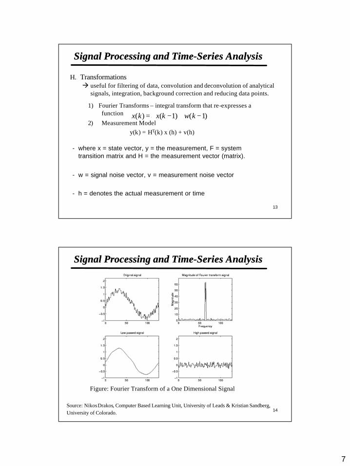
1) Fourier Transforms – integral transform that re-expresses a function
2) Measurement Modely(k) = HT(k) x (h) + v(h)
- where x = state vector, y = the measurement, F = system transition matrix and H = the measurement vector (matrix).
- w = signal noise vector, v = measurement noise vector
- h = denotes the actual measurement or time
)1()1()( −+−= kwkxkx F
14
Signal Processing and TimeSignal Processing and Time--Series AnalysisSeries AnalysisSignal Processing and TimeSignal Processing and Time--Series AnalysisSeries Analysis
Figure: Fourier Transform of a One Dimensional Signal
Source: NikosDrakos, Computer Based Learning Unit, University of Leads & Kristian Sandberg, University of Colorado.
8
15
Signal Processing and TimeSignal Processing and Time--Series AnalysisSeries AnalysisSignal Processing and TimeSignal Processing and Time--Series AnalysisSeries Analysis
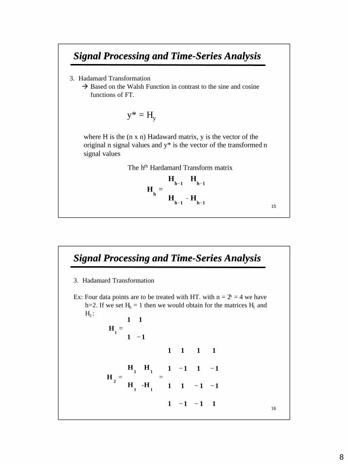
3. Hadamard Transformationà Based on the Walsh Function in contrast to the sine and cosine
functions of FT.
where H is the (n x n) Hadaward matrix, y is the vector of the original n signal values and y* is the vector of the transformed n signal values
y* = Hy
The hth Hardamard Transform matrix
=
−−
−−
1h1h
1h1h
hHH
HHH
-
16
Signal Processing and TimeSignal Processing and Time--Series AnalysisSeries AnalysisSignal Processing and TimeSignal Processing and Time--Series AnalysisSeries Analysis
3. Hadamard Transformation
Ex: Four data points are to be treated with HT. with n = 2h = 4 we have h=2. If we set H0 = 1 then we would obtain for the matrices H1 and H2 :
-
−=
11
11H
1
−−
−−
−−=
=
1111
1111
1111
1111
HH
HHH
11
11
2
9
17
Signal Processing and TimeSignal Processing and Time--Series AnalysisSeries AnalysisSignal Processing and TimeSignal Processing and Time--Series AnalysisSeries Analysis
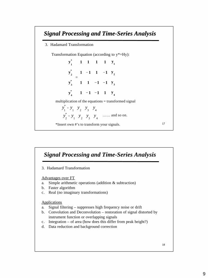
3. Hadamard Transformation
Transformation Equation (according to y*=Hy):
−−
−−
−−=
4
3
2
1
*
4
*3
*
2
*
1
y
y
y
y
1111
1111
1111
1111
y
y
y
y
multiplication of the equations = transformed signal
…… and so on.
*Insert own #’s to transform your signals.
4321*1
yyyyy +++=
4321*2
yyyyy +++=
18
Signal Processing and TimeSignal Processing and Time--Series AnalysisSeries Analysis
3. Hadamard Transformation
Advantages over FTa. Simple arithmetic operations (addition & subtraction)b. Faster algorithmc. Real (no imaginary transformations)
Applicationsa. Signal filtering – suppresses high frequency noise or driftb. Convolution and Deconvolution – restoration of signal distorted by
instrument function or overlapping signalsc. Integration – of area (how does this differ from peak height?)d. Data reduction and background correction
10
19
TimeTime--Series AnalysisSeries Analysis
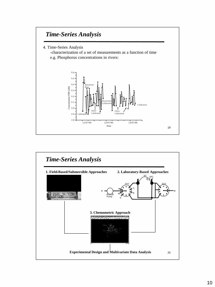
4. Time-Series Analysis-characterization of a set of measurements as a function of timee.g. Phosphorus concentrations in rivers:
17:00 03:00 13:00 23:004.8
4.9
5.0
5.1
5.2
5.3
5.4
5.5
5.6
Filter/Calibration
Filter/Calibration
Downtime/Filter
Downtime/Calibration
Calibration
Calibration
13/07/0012/07/0011/07/00
Con
cent
ratio
n FR
P (u
M)
Date
20
TimeTime--Series AnalysisSeries Analysis
W
Pump
B
S
A
W
C
B
SV1 SV2
+-SC SFC
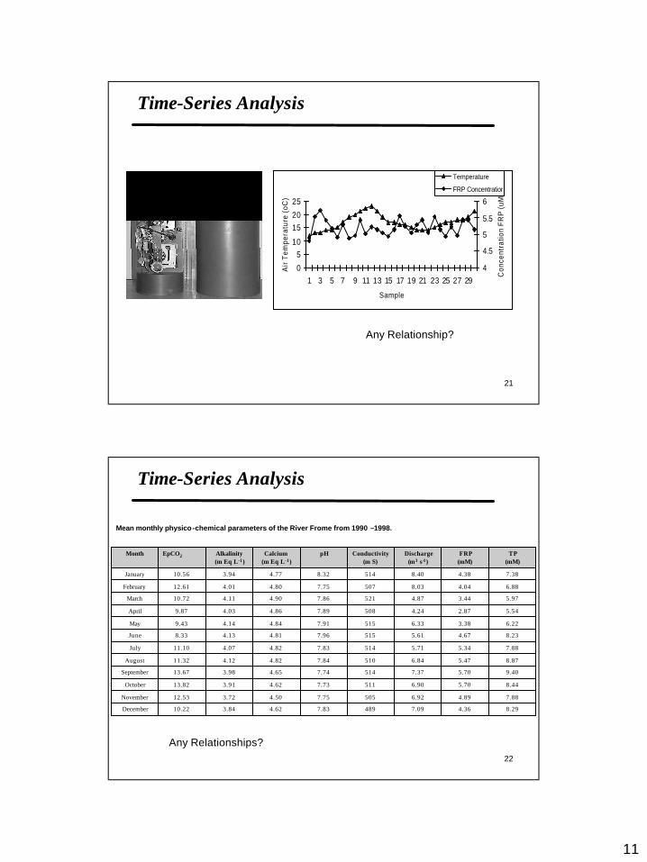
1. Field-Based/Submersible Approaches 2. Laboratory-Based Approaches
3. Chemometric Approach
Experimental Design and Multivariate Data Analysis
11
21
0
510
1520
25
1 3 5 7 9 11 13 15 17 19 21 23 25 27 29
SampleA
ir T
empe
ratu
re (o
C)
4
4.5
5
5.5
6
Con
cent
ratio
n FR
P (u
M)
Temperature
FRP Concentration
TimeTime--Series AnalysisSeries Analysis
Any Relationship?
22
Mean monthly physico-chemical parameters of the River Frome from 1990 –1998.
8.294.367.094897.834.623.8410.22December
7.884.896.925057.754.503.7212.53November
8.445.706.905117.734.623.9113.82October
9.405.707.375147.744.653.9813.67September
8.875.476.845107.844.824.1211.32August
7.885.345.715147.834.824.0711.10July
8.234.675.615157.964.814.138.33June
6.223.386.335157.914.844.149.43May
5.542.874.245087.894.864.039.87April
5.973.444.875217.864.904.1110.72March
6.884.048.035077.754.804.0112.61February
7.384.388.405148.324.773.9410.56January
TP(µ M)
FRP(µ M)
Discharge(m3 s-1)
Conductivity(µ S)
pHCalcium(m Eq L-1)
Alkalinity(m Eq L-1)
EpCO2Month
TimeTime--Series AnalysisSeries Analysis
Any Relationships?
12
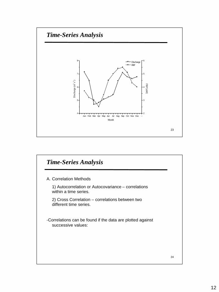
23
Jan Feb Mar Apr May Jun Jul Aug Sep Oct Nov Dec --4
5
6
7
8
Discharge FRP
Month
Dis
char
ge (m
3 s-1
)
2
3
4
5
6
FRP [uM
]
TimeTime--Series AnalysisSeries Analysis
24
TimeTime--Series AnalysisSeries Analysis
A. Correlation Methods
1) Autocorrelation or Autocovariance – correlations within a time series.
2) Cross Correlation – correlations between two different time series.
-Correlations can be found if the data are plotted against successive values:
13
25
TimeTime--Series AnalysisSeries Analysis
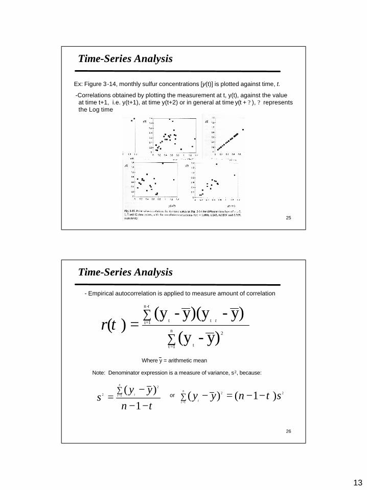
Ex: Figure 3-14, monthly sulfur concentrations [y(t)] is plotted against time, t.
-Correlations obtained by plotting the measurement at t, y(t), against the value at time t+1, i.e. y(t+1), at time y(t+2) or in general at time y(t + ? ), ? represents the Log time
26
TimeTime--Series AnalysisSeries Analysis
- Empirical autocorrelation is applied to measure amount of correlation
∑
∑
=
= += n
1t
2
t
-n
1t tt
y)-(yy)-y)(y-(y
)(τ
ττr
Where y = arithmetic mean
Note: Denominator expression is a measure of variance, s2, because:
τ−−−
=∑
=
1)(
1
2
2
nyy
sn
t t or ∑=
−−=−n
t tsnyy
1
22 )1()( τ
14
27
TimeTime--Series AnalysisSeries Analysis
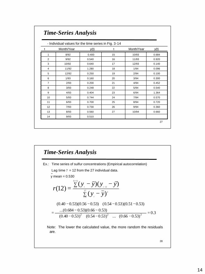
- Individual values for the time series in Fig. 3-14
t Month/Year y(t) t Month/Year y(t)
0.5109/9314
0.66010/94270.5608/9313
0.3609/94260.7307/9312
0.7208/94250.7006/9311
0.5707/94240.7445/9310
1.3646/94230.4044/939
0.5405/94220.2483/938
0.4524/94210.2002/937
0.3003/94200.1601/936
0.1002/94190.25012/925
0.0961/94181.28011/924
0.14012/93170.64010/923
0.92011/93160.5409/922
0.68410/93150.4008/921
28
TimeTime--Series AnalysisSeries Analysis
Ex.: Time series of sulfur concentrations (Empirical autocorrelation)
Lag time ? = 12 from the 27 individual data.
y mean = 0.530
∑
∑
=
−
= +
−−−
= 27
1
2
12
1 12
)())((
)12(t t
Lt
t tt
yyyyyy
r
3.0)53.066.0(...)53.054.0()53.040.0(
)53.066.0)(53.0684.0...()53.051.0)(53.054.0()53.056.0)(53.040.0(
222 =−++−+−
−−+
−−+−−
=
Note: The lower the calculated value, the more random the residuals are.
15
29
TimeTime--Series AnalysisSeries Analysis
Cross–Correlation
- Crorrelation between two different time series, y(t) and x(t)
- Empirical cross-correlation:
∑ ∑
∑
= =
−
= −=n
t
n
t
n
t
tt
ttxy yx
yxr
1 1
||
1
22)(
τ
ττ
30
TimeTime--Series AnalysisSeries Analysis
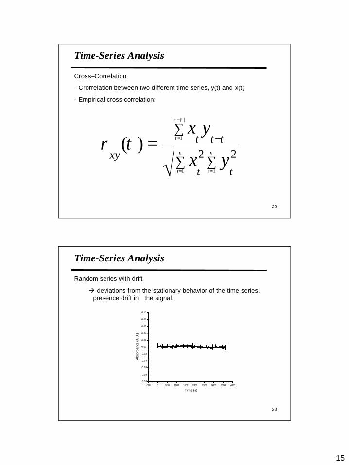
Random series with drift
à deviations from the stationary behavior of the time series, presence drift in the signal.
-500 0 500 1000 1500 2000 2500 3000 3500 4000
-0.10
-0.08
-0.06
-0.04
-0.02
0.00
0.02
0.04
0.06
0.08
0.10
Abs
orba
nce
(A.U
.)
Time (s)
16
31
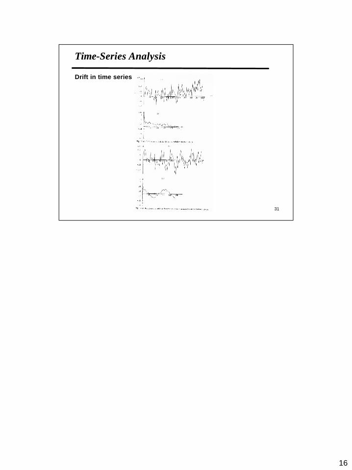
TimeTime--Series AnalysisSeries Analysis
Drift in time series