signal and image analysis using chaos theory...
TRANSCRIPT

1
SIGNAL AND IMAGE ANALYSIS USING CHAOS THEORY AND FRACTAL GEOMETRY
Wlodzimierz Klonowski Lab. of Biosignal Analysis Fundamentals
Institute of Biocybernetics and Biomedical Engineering, Polish Academy of Sciences 02-109 Warsaw, 4 Trojdena St., Poland; e-mail: [email protected]
Abstract. Fractal geometry has proven to be a useful tool in quantifying the structure of a wide range of idealized and naturally occurring objects, from pure mathematics, through physics and chemistry, to biology and medicine. In the past few years fractal analysis techniques have gained increasing attention in signal and image processing, especially in medical sciences, e.g. in pathology, neuropsychiatry, cardiology. This article intends to describe fractal techniques and its applications. We concentrate on applications of chaos theory and fractal geometry in biosignal and biomedical image analysis.
Key words: Fractals; Nonlinear Dynamics; Chaos, deterministic; Fractal dimension, Signal analysis; Pattern recognition; Morphometry,
The hardest thing in the world to understand is the income tax. -- Albert Einstein
1. Introduction
1.1. Fractals and deterministic chaos
The term fractal (from Latin fractus - irregular, fragmented) applies to objects in space or fluctuations in time that possess a form of self-similarity and cannot be described within a single absolute scale of measurement. Fractals are recurrently irregular in space or time, with themes repeated like the layers of an onion at different levels or scales. Fragments of a fractal object or sequence are exact or statistical copies of the whole and can be made to match the whole by shifting and stretching. Sequential fractal scaling relationships are observed in many physiological processes. Spatial structures of many living systems are fractal. Fractal geometry has evoked a fundamentally new view of how both nonliving and living systems result from the coalescence of spontaneous self-similar fluctuations over many orders of time and how systems are organized into complex recursively nested patterns over multiple levels of space.
A system can be anything that has more than one part. The system is said to be dynamical when system's states, including the relationships (interactions) between its parts (elements), change with time. Rules that describe these changes are called dynamics. If the interactions are nonlinear, i.e. if the result of action of one element onto another is not directly proportional to the action itself (the reaction is not simply proportional to the applied stimulus), the system is said to show nonlinear dynamics. For example, in classical mechanics the result of a force acting onto a body is an acceleration of the body proportional to the acting force because body’s mass is constant and does not depend on the body’s velocity; in relativistic mechanics this is not true since body’s mass does depend on its velocity. Simple systems with nonlinear dynamics often generate very random-like effects known as chaos. The paradox of chaos is that it is deterministic i.e. results from a dynamic that is not govern by laws of probability. Because of extreme sensitivity to initial conditions and system's parameters chaotic system may seem to behave completely randomly. But there is an order underlying such behavior. For example, random numbers from a computer generator
W.Klonowski Signal and Image Analysis Using Chaos Theory and Fractal Geometry
2
appear to lack any degree of order, when in fact the numbers are produced in a very ordered and deterministic fashion. Probability of a random number generator producing the string “1010…” is exactly the same as the probability of any other particular string with half 1’s, half 0’s. Both string have the same statistics and thus the same probability of occurrence, although one is regularly patterned and other is not [2]. Randomness is relative and context dependent - the definition of randomness as ‘lacking all order’ has no real meaning. Unlike random systems, systems governed by deterministic chaos may be rather easily controlled. Methods of nonlinear dynamics and deterministic chaos theory provide tools for analyzing and modeling chaotic phenomena and may supply us with effective quantitative descriptors of underlying dynamics and of system’s fractal structure.
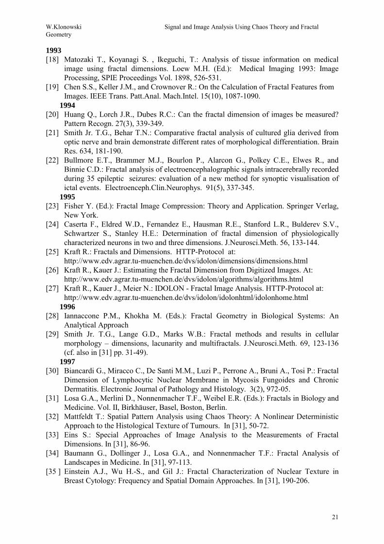
Dynamical system moves towards one or more attractors which can be thought of as the system's equilibrium states in the system’s phase space. Systems that give rise to deterministic chaos have chaotic or strange attractors. Here chaos theory intimately relates to fractal geometry since strange attractors turn out to be fractals. But building up the phase space for a system poses several problems – the data characterizing the system (e.g. amplitudes of a signal produced by the system in consecutive moments of time) have to be embedded in the properly chosen multidimensional space. On the other hand, processes in chaotic systems often produce structures or signals that are fractal in real space or in time, respectively (Fig. 1).
At first glance, using a dynamical method to analyze static objects, such as gray value images, might seem to be a contradiction. However, we are able to apply dynamical methods if we are able to extract from a static object a sequence of data representing the ‘dynamical’ behavior of the object [34]. 1. 2. Fractals in biomedicine
It is not surprising that the methods of fractal mathematics, which allow quantification of structure or pattern across many spatial or temporal scales, could be useful in many biomedical applications including:
��biosignal analysis, pattern recognition; ��radiological and ultrasonographic image analysis; ��cellular morphometry, nuclei (chromatin) organization, gene expression; ��physiological and pathological states of brain and nervous system, heart and
circulatory system, lungs and pulmonary system; ��analysis of connective tissue, epithelial-stromal tissue interface, tissue-remodeling; ��biological design, angiogenesis, evolutionary patterns, morphogenesis, spatio-temporal
tree structures, vessel branching; ��structure, complexity and chaos in tumors; ��membranes and cell organelles during growth and death (apoptosis, necrosis); ��aging, immunological response, autoimmune and chronic diseases; ��complexity, self-organization and chaos in metabolic and signaling pathways; ��structure of biopolymers (proteins, nucleic acids);
Several interesting examples of applications of fractals in biology and medicine are given in the book edited by Losa et al. [31]. Biology is the discipline distinguished among all sciences by the interplay of randomness (playing an important role e.g. in evolution), nonlinearity (which plays an essential role in the creation of forms) and complexity (irreversible, dissipative fractal structures playing a determining role in generating and shaping life forms).

W.Klonowski Signal and Image Analysis Using Chaos Theory and Fractal Geometry
3
2. Fractal geometry and fractal dimension
Fractal dimension is a measure of how ‘complicated’ a self-similar figure is. In a rough sense, it measures ‘how many points’ lie in a given set. A plane is ‘larger’ than a line, while Sierpinski triangle (cf. 2.1) sits somewhere in between these two sets. On the other hand, all three of these sets have the same number of points in the sense that each set is uncountable. Somehow, though, fractal dimension captures the notion of ‘how large a set is’.
Fractal geometry can be considered as an extension of Euclidean geometry. Conventionally, we consider integer dimensions which are exponents of length, i.e., surface = length2 or volume = length3. The exponent is the dimension. Fractal geometry allows for there to be measures which change in a non-integer or fractional way when the unit of measurements changes. The governing exponent D is called fractal dimension.
Fractal object has a property that more fine structure is revealed as the object is magnified, similarly like morphological complexity means that more fine structure (increased resolution and detail) is revealed with increasing magnification. Fractal dimension measures the rate of addition of structural detail with increasing magnification, scale or resolution. The fractal dimension, therefore, serves as a quantifier of complexity. Ideal points have Euclidean dimension of 0, ideal lines of 1, and perfectly flat planes of 2. However, collection of real points have dimension greater than 0, real lines greater than 1, real surfaces greater than 2, etc. At each level, as the dimensions of an object move from one integer to the next, the complexity of the object increases; it becomes more area filling from 1 to 2, more volume-filling from 2 to 3, etc. [7]. Euclidean or non-fractal (points, lines, circles, cubes, etc.) may be viewed as fractal objects with the lowest complexity (integer fractal dimensions) within their respective dimension domains (0 to 1, 1 to 2, etc.) [29]. Natural objects are often rough and are not well described by the ideal constructs of Euclidian geometry [7].
One familiar example of naturally occurring fractal curves is coastline. Since all of the curve’s features that are smaller than the size of the measuring tool will be missed, whatever is the size of the measuring tool selected, therefore the result obtained depends not only on the coastline itself but also on the length of the measurement tool. The use of fractional power in the measurements compensates for the details smaller than the size of measuring tool - fractal dimension is the unique fractional power that yields consistent estimates of a set’s metric properties. Because it provides the correct adjustments factor for all those details smaller than the measuring device, it may also be viewed as a measurement of the shape’s roughness [2].
The fractal dimension of an object provides insight into how elaborate the process that generated the object might have been, since the larger the dimension the larger the number of degrees of freedom likely have been involved in that process [2].
2. 1. Mathematical fractals - self-similarity
Objects considered in Euclidean geometry are sets embedded in Euclidean space and object’s dimension is the dimension of the embedding space. One is also accustomed to associate what is called topological dimension with Euclidean objects - everybody knows that a point has dimension of 0, a line has dimension of 1, a square is 2-dimensional, and a cube is 3-dimensional. The topological dimension is preserved when the objects are transformed by a homeomorphism. One cannot use topological dimension for fractals, but instead has to use what is called Hausdorff-Besikovitch dimension, commonly known as fractal dimension.
In fact, a formal definition of a fractal says that it is an object for which the fractal dimension is greater than the topological dimension. But this definition is too restrictive. An
W.Klonowski Signal and Image Analysis Using Chaos Theory and Fractal Geometry
4
alternative definition uses the concept of self-similarity – a fractal is an object made of parts similar to the whole. The notion of self-similarity is the basic property of fractal objects.
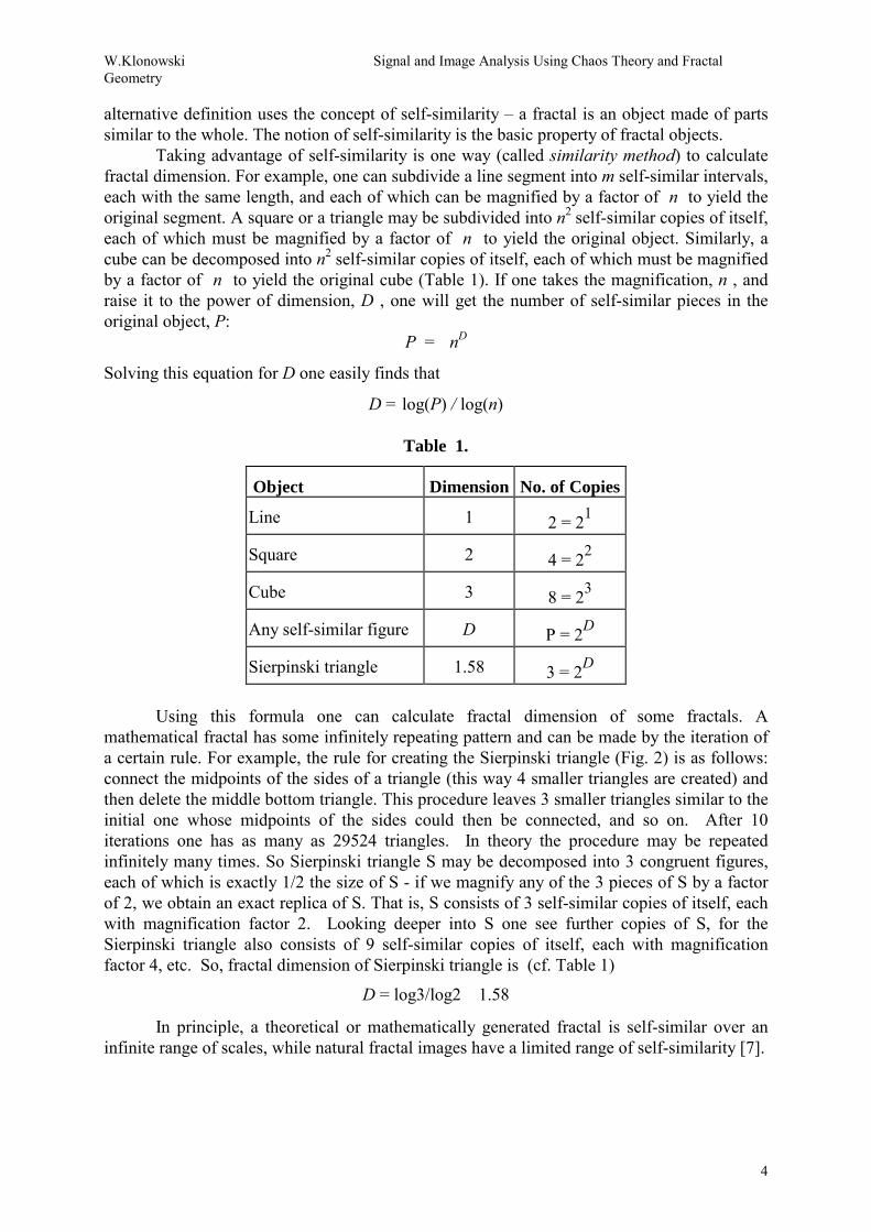
Taking advantage of self-similarity is one way (called similarity method) to calculate fractal dimension. For example, one can subdivide a line segment into m self-similar intervals, each with the same length, and each of which can be magnified by a factor of n to yield the original segment. A square or a triangle may be subdivided into n2 self-similar copies of itself, each of which must be magnified by a factor of n to yield the original object. Similarly, a cube can be decomposed into n2 self-similar copies of itself, each of which must be magnified by a factor of n to yield the original cube (Table 1). If one takes the magnification, n , and raise it to the power of dimension, D , one will get the number of self-similar pieces in the original object, P:
P = nD
Solving this equation for D one easily finds that
D = log(P) / log(n)
Table 1.
Object Dimension No. of Copies
Line 1 2 = 21
Square 2 4 = 22
Cube 3 8 = 23
Any self-similar figure D P = 2D
Sierpinski triangle 1.58 3 = 2D
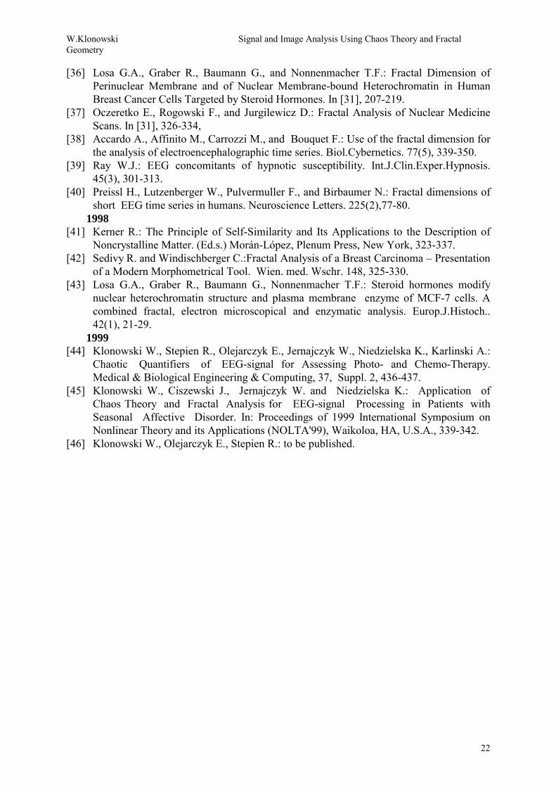
Using this formula one can calculate fractal dimension of some fractals. A mathematical fractal has some infinitely repeating pattern and can be made by the iteration of a certain rule. For example, the rule for creating the Sierpinski triangle (Fig. 2) is as follows: connect the midpoints of the sides of a triangle (this way 4 smaller triangles are created) and then delete the middle bottom triangle. This procedure leaves 3 smaller triangles similar to the initial one whose midpoints of the sides could then be connected, and so on. After 10 iterations one has as many as 29524 triangles. In theory the procedure may be repeated infinitely many times. So Sierpinski triangle S may be decomposed into 3 congruent figures, each of which is exactly 1/2 the size of S - if we magnify any of the 3 pieces of S by a factor of 2, we obtain an exact replica of S. That is, S consists of 3 self-similar copies of itself, each with magnification factor 2. Looking deeper into S one see further copies of S, for the Sierpinski triangle also consists of 9 self-similar copies of itself, each with magnification factor 4, etc. So, fractal dimension of Sierpinski triangle is (cf. Table 1)
D = log3/log2 � 1.58
In principle, a theoretical or mathematically generated fractal is self-similar over an infinite range of scales, while natural fractal images have a limited range of self-similarity [7].
W.Klonowski Signal and Image Analysis Using Chaos Theory and Fractal Geometry
5
2. 2. Natural fractals - statistical self-similarity
The similarity method for calculating fractal dimension works for a mathematical fractal, which like Sierpinski triangle is composed of a certain number of identical versions of itself. It is not true for natural objects. Such objects show only statistical self-similarity [25].
A mathematical fractal has an infinite amount of details. This means that magnifying it adds additional details, so increasing the overall size. In non-fractals, however, the size always stays the same, no matter of applied magnification. If one makes a graph log(fractal’s size) against log(magnification factor) one gets a straight line. For non-fractals this line is horizontal since the size (e.g. length of a segment, area of a triangle, volume of a cylinder) does not change. For fractal object the line is no longer horizontal since the size increases with magnification. The geometric method of calculating fractal dimension finds that fractal dimension can be calculated from the slope of this line. Both the similarity method and geometric method of calculating fractal dimension require measuring of fractal size. For many fractals it is practically impossible. For these fractals one applies box-counting method. Consider putting the fractal on a sheet of graph paper, where the side of each square box is size h. Instead of finding the exact size of the fractal one counts the number of boxes that are not empty, i.e. each box that contains at least one pixel of the fractal under consideration. Let number of these boxes be P. Making the boxes smaller gives more detail, which is the same as increasing the magnification. In fact, the magnification, n, is equal to 1/h. In similarity method the formula for fractal dimension is D = log(P)/log(n). With box-counting method
D = log(P)/log(1/h) = - log(P)/log(h)
Making h smaller will make the dimension more accurate. For 3-D fractals one can do the same with cubes instead of squares, and for 1-D fractals one can use line segments.
For example, let’s calculate the fractal dimension of the Box fractal (Fig. 3). Using box-counting method, we put the fractal on a sheet of graph paper, we use boxes with sizes 1/3 and 1/9. In the first case (Fig. 3a.), 5 boxes are not empty; in the second case (Fig. 3b.), there are 25 non-empty boxes, etc. In the first case D = log (5)/log[1/(1/3)] = 1.46; for the second case the answer is the same, which means that our dimension is accurate. For natural fractals the procedure is more complicated than in the case of Box fractal, but still the number of boxes needed to cover a fractal set obeys the power law. The logarithm of the box size (usually in pixel units [13]) is plotted on the horizontal axis and the logarithmic total area of boxes containing at least one pixel belonging to the considered fractal is plotted on the vertical axis. The fractal dimension, called in this case the box dimension is determined from the slope of the regression line {log(h), -log(P)}. Three pairs of data may be enough. The slope of the curve is the estimation of box dimension D [19]. The so-called ‘sandbox’ or cumulative-mass method ([14, 24, 29], cf. also 2.4) is a variant of the box-counting method. Living bodies are also ‘made of fractals’ and the pulmonary system is the best example. It is composed of tubes, through which the air passes into microscopic sacks called alveoli. Trachea, the main tube of the system, splits into two smaller tubes, called the bronchi, which lead to different lungs. Bronchi in turn split into smaller tubes, which are even further split. This splitting continues further and further until the smallest tubes, called the bronchioles, which lead into the alveoli. This description is similar to that of a typical fractal, especially so-called fractal canopie, which is formed by splitting lines (Fig. 4). Another supporting evidence that lungs are fractal comes from measurements of the alveolar area, which was found to be 80 m2 with light microscopy and 140 m2 at higher magnification with electron microscopy.

W.Klonowski Signal and Image Analysis Using Chaos Theory and Fractal Geometry
6
The increase in size with magnification is one of the properties of fractals. Fractal structure of the bronchial tree is imposed by optimization of resource utilization requirements in the lung, such as efficient distribution of blood and air. Thus, the morphology of the lung is directly related to its function and changes in its structure can be linked to dysfunction. Since the bronchial tree is a fractal structure, its fractal dimension can be used as a tool for the detection of structure changes and quantification of lung diseases. A quantitative computerized method, which provides accurate discrimination between chest radiographs with positive findings of interstitial disease patterns and normal chest radiographs may increase the efficacy of radiological screening of the chest and the utility of digital radiographic systems.
Similar splitting can also be found in blood vessels. Arteries, for example start with the aorta, which splits into smaller blood vessels. The smaller ones split as well, and the splitting continues until the capillaries, which, just like alveoli, are extremely close to each other. Because of this, blood vessels can also be described by fractal canopies.
Biological fractal structures like lungs and the vascular bed represent probably optimal design for their particular functions, like air flow or blood flow, respectively. It may well be that the fractal, dendritic trees of neurons are also optimally designed , but in this case for the flow of the most important commodity: information [29]. The surface of human brain contains a large number of folds. Its fractal dimension is between 2.73 – 2.79, the highest in the animal kingdom.
Folding of the nasal membrane allow better sensing of smells by increasing the sensing surface. However, in humans this membrane is less folded than in other animals, so making humans less sensitive to smells. The membranes of cell organelles, like mitochondria and the endoplasmic reticulum, are also folded. Fractal dimensions of some biological structures are given in Table 2.
Fractals can also be found in various biomolecules, like DNA and proteins.
Table 2.
Anatomical Structure D
Bronchial Tubes very close to 3
Arteries 2.7
Human brain 2.73 – 2.79
Alveolar Membrane 2.17
Mitochondrial Membrane (outer) 2.09
Mitochondrial Membrane (inner) 2.53
Endoplasmic Reticulum 2.72
2. 3. Brownian self-similarity, self-affinity, and spectral fractal dimension
Natural objects like coastlines or roots do not show exactly the same shape but look quite similar when they are scaled down. Due to their statistical scaling invariance they are called statistical self-similar. The miniature copy of a structure may be distorted e.g. skewed;
W.Klonowski Signal and Image Analysis Using Chaos Theory and Fractal Geometry
7
for this case there is the notion of self-affinity; within a self-affine structure the scaling factor is not constant [25] (Fig. 5).
Statistical self-similarity and self-affinity is often called Brownian self-similarity. An object showing this property may be decomposed into parts which looks much alike the whole object but are made up of randomly located (instead of being fixed) smaller parts, which in turn may be decomposed into still smaller randomly located parts etc. Virtually all fractals encountered in physical models have two additional properties: 1st - each segment is statistically similar to all others; 2nd - they are statistically invariant over wide transformation scale. The path of a particle exhibiting Brownian motion, observed in shorter and shorter time intervals, is the canonical example of this type of fractal, and so called fractal Brownian functions are a mathematical generalization of Brownian motion [2]. For a one-dimensional Brownian motion the mean square displacement is
<ξ2> = 2Dt2H where D is diffusion constant and H is the Hurst exponent that represents a measure of smoothness of a fractal object – a low value of H is related to high roughness, while a high H near 1 is connected with a high smoothness. The scaling exponent H helps us to distinguish different types of stochastic processes. H=½ indicates that the process represents a classical Brownian motion that allows the occurrence of all step lengths with the same probability; for values H<½ the motion is called persistent (continuing in the same direction more often than if it was completely random), while for H>½ – antipersistent (changing direction more often than if it was completely random) [34]. Fractal Brownian function, VH(x) (where x is a q-dimensional vector of independent variables) has zero-mean Gaussian increment with variance:
<[VH(x+δ) - VH(x)]2> � xδx2H where H є (0,1) denotes Hurst exponent. For a one-dimensional fractal Brownian function the fractal dimension D of the graph described by this function is
D = 2 – H.
Further, VH(x) has a random-phase Fourier spectrum with power FH(f) such that
FH � f –β In one topological dimension H is related to β by
β = 2H + 1
In two topological dimensions
β = 2H + 2
A fractal Brownian function VH(x) defines q-dimensional fractal Brownian surface. Spectral density of a fractal Brownian function is proportional to f—2H-1. Kube and Pentland [6] demonstrated that a fractal Brownian surface with power spectrum proportional to f –β
produces an image with power spectrum proportional to f 2–β. So one can use the spectral falloff of the image to predict the fractal dimension of the surface [6]. If image’s power spectrum is modeled as 1/f β noise, for statistically self-affine fractal Brownian motion the spectral exponent β is related to a fractal similarity dimension (spectral fractal dimension) DS by the equation
DS = (7 – β) / 2
Power spectra are determined from images’ two-dimensional Fourier transforms [35].

W.Klonowski Signal and Image Analysis Using Chaos Theory and Fractal Geometry
8
Second-order properties of a stochastic process such as auto-covariance and the spectrum are also available for examining self-similarity and measuring its indices; this is especially easy for stochastic processes on a real line (one-dimensional point processes). Fractal dimension and the Hurst number are estimated objectively by maximizing a spectral log likelihood [13].
2.4. Fractal analysis as statistical analysis
Certain structures like quasi-crystals or network glasses display at any magnification scale similar, although never strictly identical images. Even in the apparently totally disordered systems such as glasses or polymer networks we may observe statistical self-similarity (repetition of characteristic local structures and certain typical correlations between them) if we use probabilistic description of the network. This is the most characteristic feature of the self-similarity: the fundamental information about the structure of a complicated system is contained already in quite small samples, and we can reproduce all the essential features by adding up and repeating similar subsets ad infinitum even if they are not strictly identical like in crystalline lattice, but just very much alike like in quasi crystals or network glasses [41].
It should be emphasized that D is a descriptive, quantitative measure; it is a statistic, in the sense that it represents an attempt to estimate a single-valued number for a property (complexity) of an object with a sample of data from the object. One can, for example, view D in much the same way that thermodynamics might view intense measures such as temperature. That is, as a measure of a property of some object or material, even though unlike in the case of temperature not much is known about the underlying mechanisms leading to this value. D is not a unique, sufficient measure; for example, two objects may appear visually very different from one another and yet have the same fractal dimension [29].
2.5. Length- and mass-related fractal dimension of image border
There are two basic approaches to measuring the fractal dimension of image border - length-related, when the size of a pixel side becomes the unit of length (the resultant D is called the capacity dimension) and mass-related methods, when the individual border pixel becomes the unit of mass (the ‘sandbox’ or the cumulative mass dimension) [29]. For example, the box-counting method (cf. 2.2) is mass-related and should not be confused with the length-related grid method (cf. 4.2) that sometimes is also called ‘box-counting’ method. Because of fractal self-similarity, in length-related methods the magnitude of the resultant measure (perimeters, etc.) increases as the measuring element (ruler, etc.) decreases in size. The relevant power relationship is L(e) = Fes where L(e) is the equivalent perimeter as a function of the resolving element, e , F is a prefactor, and s is the slope of the plot of log[L(e)] vs. log(e). Then length fractal dimension D = 1 – s. Since s is negative and │s│ is less than 1, D is between 1 and 2 [29] (cf. Fig. 6). The mass-oriented methods involve counting of border pixels contained in a sampling region (e.g. disc diameter) as a function of the sizes of the sampling regions. One centers boxes or circles (the result is the same irrespective of the shape used) of different sizes at many randomly located points on the border and counts the number of border pixels contained within each box or circle. The log of the number of pixels within each box or circle is plotted against the log of the measuring element (edge size, diameter). A fractal model gives a line with a positive slope, which is the D for that object. The power relationship plotted is µ(r) = ArD

W.Klonowski Signal and Image Analysis Using Chaos Theory and Fractal Geometry
9
where µ(r) is the number of pixels (mass) in a box of size r, r is the circle diameter or box-edge length, A is a prefactor, and D is the slope of the plot of log[µ(r)] vs. log(r) and D is the mass fractal dimension [29] (cf. Fig. 6). Mass measure provide another and often different value(s) of D for the same object analyzed with length measures. For Euclidean objects and mathematical fractals the length and mass fractal D are theoretically the same, but in practice they may differ slightly due to the less than perfect resolution in the digitized images [29]. With natural fractals the two Ds are often different, with the mass fractal D value usually being the larger. There is another distinguishing property of fractal objects. They may have either uniformly or non-uniformly distributed pixels; the global length-derived Ds may be the same for two fractals looking very different, but mass-derived Ds in such cases are often unequal [29]. The mass measures provide more information about the fractal object than the length measures [4]. Mass measures also lead to the concepts of lacunarity and multifractals discussed below. 2.6. Lacunarity
The properties and characteristics of a fractal set are not completely determined by its fractal dimension D. Indeed, fractals that have the same fractal dimension may look very different - they have different ‘texture’, more specifically, different lacunarity (cf. Fig. 6). Lacunarity is a counterpart to the fractal dimension that describes the texture of a fractal. It is strongly related with the size distribution of the holes on the fractal and with its deviation from translational invariance. Roughly speaking, if a fractal has large gaps or holes it has high lacunarity; on the other hand, if a fractal is almost translationally invariant it has low lacunarity.
Lacunarity (from the Latin lacuna for lack, gap or hole) measures structural variation or inhomogenities that may be manifested by ‘texture’ [29]. In a restrictive sense it is a measure of the lack of rotational or translational invariance. In a more general sense, lacunarity is a measure of non-uniformity (heterogeneity) of structure or the degree of structural variance within an object. Lacunarity is usually defined in terms of mass related distribution. A common procedure is to calculate the mean and variance (or standard deviation) of some measure, e.g. the mass (number of pixels) in a box of a given size. For fractals, the result of this calculation is a strong function of a scale; thus to obtain a single number for lacunarity the variance calculations must be normalized. This can be done, for example, by dividing the variance by the square of mean at each scale. Alternatively, one can divide the standard deviation by the mean at each scale to give what in statistics is called the coefficient of variation or relative dispersion (the former result is simply the square of the latter). For a self-similar object the coefficient of variation should be constant with scale, since the form of the object at large scales is a magnified version of its form at small scales. That is, the object looks the same at all scales. Therefore, the mean and standard deviation would scale up in the same proportion and their ratio would be the constant, which is equal to lacunarity. Furthermore, the variability of the mass measure about its average value would have a constant vertical scatter when plotted in the log-log graphs (cf. Figs. 6C and 6F)) [29]. So, lacunarity may be interpreted as the width of the mass distribution functions. Lacunarity measures to the extent at which a set is not translationally invariant [14].
Lacunarity may be calculated from the fluctuations of the mass distribution function by using the gliding-box algorithm. In this method the image (set) under study is put on an underlying lattice with a mesh size equal to 2a; for instance, the underlying lattice is the array of pixels provided by the image processing system which is used to digitize the structure.
W.Klonowski Signal and Image Analysis Using Chaos Theory and Fractal Geometry
10
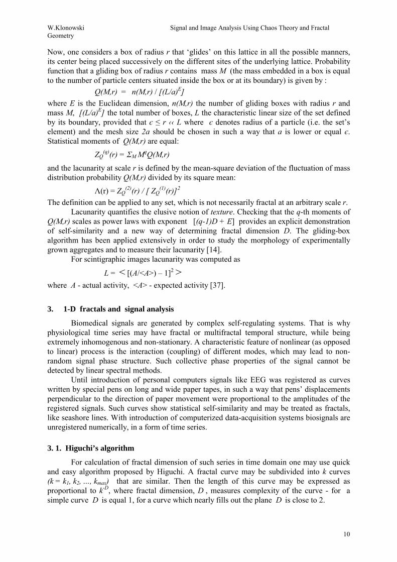
Now, one considers a box of radius r that ‘glides’ on this lattice in all the possible manners, its center being placed successively on the different sites of the underlying lattice. Probability function that a gliding box of radius r contains mass M (the mass embedded in a box is equal to the number of particle centers situated inside the box or at its boundary) is given by : Q(M,r) = n(M,r) / [(L/a)E] where E is the Euclidean dimension, n(M,r) the number of gliding boxes with radius r and mass M, [(L/a)E] the total number of boxes, L the characteristic linear size of the set defined by its boundary, provided that є ≤ r ‹‹ L where є denotes radius of a particle (i.e. the set’s element) and the mesh size 2a should be chosen in such a way that a is lower or equal є. Statistical moments of Q(M,r) are equal:
ZQ(q)(r) = ΣM MqQ(M,r)
and the lacunarity at scale r is defined by the mean-square deviation of the fluctuation of mass distribution probability Q(M,r) divided by its square mean:
Λ(r) = ZQ(2)(r) / [ ZQ
(1)(r)]2 The definition can be applied to any set, which is not necessarily fractal at an arbitrary scale r.
Lacunarity quantifies the elusive notion of texture. Checking that the q-th moments of Q(M,r) scales as power laws with exponent [(q-1)D + E] provides an explicit demonstration of self-similarity and a new way of determining fractal dimension D. The gliding-box algorithm has been applied extensively in order to study the morphology of experimentally grown aggregates and to measure their lacunarity [14].
For scintigraphic images lacunarity was computed as
L = < [(A/<A>) – 1]2 > where A - actual activity, <A> - expected activity [37].
3. 1-D fractals and signal analysis
Biomedical signals are generated by complex self-regulating systems. That is why physiological time series may have fractal or multifractal temporal structure, while being extremely inhomogenous and non-stationary. A characteristic feature of nonlinear (as opposed to linear) process is the interaction (coupling) of different modes, which may lead to non-random signal phase structure. Such collective phase properties of the signal cannot be detected by linear spectral methods.
Until introduction of personal computers signals like EEG was registered as curves written by special pens on long and wide paper tapes, in such a way that pens’ displacements perpendicular to the direction of paper movement were proportional to the amplitudes of the registered signals. Such curves show statistical self-similarity and may be treated as fractals, like seashore lines. With introduction of computerized data-acquisition systems biosignals are unregistered numerically, in a form of time series.
3. 1. Higuchi’s algorithm
For calculation of fractal dimension of such series in time domain one may use quick and easy algorithm proposed by Higuchi. A fractal curve may be subdivided into k curves (k = k1, k2, …, kmax) that are similar. Then the length of this curve may be expressed as proportional to k-D, where fractal dimension, D , measures complexity of the curve - for a simple curve D is equal 1, for a curve which nearly fills out the plane D is close to 2.

W.Klonowski Signal and Image Analysis Using Chaos Theory and Fractal Geometry
11
In computerized data-acquisition system the signal recorded on a selected channel is represented by the time series
x(1), x(2), x(3),..., x(N) where x(i) is the signal’s amplitude at the i-th moment of time (i=1,...,N) and N is the total number of points; from this one then constructs k new time series x(m,k):
x(m,k): x(m), x(m+k), x(m+2k), ... , x(m+int[(N-m)/k]* k) (m=1, 2,...,k) where int[...] denotes the greatest integer not exceeding the number in the brackets; m and k are integers indicating the initial time and the time interval respectively. For example, if N=100 and k=4 one obtains four time series:
x(1,4): x(1), x(5),..., x(97) x(2,4): x(2), x(6),..., x(98) x(3,4): x(3), x(7),..., x(99) x(4,4): x(4), x(8),..., x(100)
In Higuchi’s method the length of the curve x(m,k) is defined as:
Lm(k) = { [ |x(m+i*k)- x(m+(i-1)*k)|] * (N-1)/int[(N-m)/k)*k]} / k i=1,int [(N-m) / k]
where the term (N-1)/int[(N-m)/k)*k] is a normalization factor. Lm(k) is then averaged for all m giving the mean value of the curve length, L(k) , for given value of k. The procedure is repeated for several k and then from the log-log plot of log(L) vs. log(k) using the least-square method one obtains Higuchi’s fractal dimension of the signal, D :
D = - log[L(k)] / log(k) We have to stress that Higuchi’s fractal dimension is always between 1 and 2 since it characterizes complexity of the curve representing the signal under consideration on a 2-dimensional plane. This fractal dimensions should not be mistaken with fractal dimension of an attractor, which is calculated in the system’s phase space. Attractor dimension, e.g. correlation dimension, is usually fractal but it may be significantly greater than 2, it may provide some measure about how many relevant degree of freedom are involved in the dynamics of the system under consideration. Calculation of attractor’s fractal dimension requires previous embedding of the data in phase space, using e.g. Taken’s time delay method [44]. For Higuchi’s method construction of phase space and data embedding are not needed, the algorithm works on raw data. Also ‘classical’ fractal dimensions, used e.g. for cell contours characterization should not be confused with fractal dimension calculated in the phase space (cf. [8]).
3. 2. Examples – analysis of EEG signals
Fractal dimension has been proposed as a useful measure for the characterization of electrophysiological time series. Electroencephalogram (EEG) traces corresponding to different physiopathological conditions can be characterized by their fractal dimension, which is a measure of the signal complexity. Generally this dimension is evaluated in the phase space by means of the attractor dimension or other correlated parameters. Nevertheless, to obtain reliable values, relatively long signal intervals are needed and consequently only long-term events can be analyzed; also much calculation time is required.
Fractal methods of EEG-signal processing enabled to establish relationship between electro cortical activity and hypnotizability. Fractal dimension of EEG in the theta frequency range (3 to 8 Hz) were examined in high and low susceptible individuals. The dimensionality
W.Klonowski Signal and Image Analysis Using Chaos Theory and Fractal Geometry
12
measures suggest that individuals highly susceptible to hypnosis display underlying brain patterns associated with imagery, whereas low susceptible individuals show patterns consistent with cognitive activity (i.e. mental math) [39].
Using time series of different length it is possible to show, that there is a monotonous relation between fractal dimension and the number of data-points. Preissl et al. [40] investigated what the pointwise dimension of electroencephalographic time series can reveal about underlying neuronal generators. Cortical activity can be considered as the weighted sum of a finite number of oscillations (plus noise). The correlation dimension of finite time series generated by multiple oscillators increases monotonically with the number of oscillators. A reliable estimate of the pointwise dimension of the raw EEG signal can be calculated from a time series of a few seconds duration, which for EEG-signals is still rather long. These results indicate that the pointwise dimension on the basis of such raw EEG signals allows conclusions regarding the number of independently oscillating networks in the cortex [40]. Pointwise dimension is calculated in system’s phase space not directly in the time domain as e.g. Higuchi’s fractal dimension.
It is feasible to use fractal dimension as a tool to characterize the complexity for short electroencephalographic time series. But to analyze events of brief duration it is necessary to make calculations directly in the time domain, using e.g. Higuchi’s algorithm. Fractal analysis allows investigating relevant EEG events shorter than those detectable by means of other linear and non-linear techniques [38].
For example, we investigated possible influence of magnetic field on human brain by analysing EEG-signal using Higuchi’s method. No influence of magnetostimulation could be noticed while inspecting EEG-recordings with the naked eye. Linear methods like FFT analysis did not reveal any evident changes indicating possible influence of magnetostimulation. Calculation of fractal dimension of EEG-signal clearly demonstrates an influence of magnetic field on the brain [46]. Fractal dimension was also used to assess influence of phototherapy on patients suffering with Seasonal Depression (Seasonal Affective Disorder, SAD); again, EEG-signal assessing with naked specialist eye or using linear methods did not reveal any evident changes, but calculation of D demonstrates influence of applied phototherapy (Fig. 7).
4. 2-D fractals and image analysis
A digitized image is a pattern stored as a rectangular data matrix. It is distinguished between binary images, grayscale images and color images. Binary images are matrices where pixels belonging to the pattern are stored as 1, pixels from the background are stored as 0. The storage may also be vice versa. On a video screen the 1-pixels are rendered as black, the 0-pixels as white or again vice versa. Binary images are said to have a depth of 2 values i.e. each pixel has value 1 (‘black’) or 0 (‘white’), or vice versa. Grayscale images are matrices where the matrix elements can take on values from 0 to 255. The rendering on a video screen is a presentation of the values from white (0) to black (255). Most color images are overlays of three grayscale images [26].
4.1. Landscapes - application of 1-D fractal analysis to 2-D patterns
It is possible to transform a 2-D pattern in such a way to obtain a 1-D pattern, which may then be analyzed using methods applied for signal analysis. For example, starting with some gray level images, first by proper segmentation binary images are produced. Then one

W.Klonowski Signal and Image Analysis Using Chaos Theory and Fractal Geometry
13
takes a strip of the binary image total length of N pixels and height of M pixels, with N several times greater than M. At each point of the long axis, denoted as t � [1, N], the fraction of ‘white’ pixels in the column orthogonal to the long axis is calculated:
x1(t)=M1(t)/M � [0, 1]
where M1(t) denotes the number of white pixels in the t-th column. The resulting series of N rational numbers x1(t) serves as input for the subsequent ‘signal analysis’. Such approach was adapted for example by Mattfeld [32] for analysis of histological texture of tumors. He analyzed microscopic images of fibrous mastopathy and of invasive ductal mammary cancer, with epithelial component represented as white and pore space as black (Fig. 8). Produced signals were undergone analysis using linear methods (autocorrelation, power spectra) and chaos theory methods (attractor correlation dimension in phase space), showing that nonlinear methods give possibility to differentiate between two kinds of tumors and that these differences may have some biological justifications (Fig. 9).
In a variation of this method for a binary picture one first counts black (or, respectively, white) pixels in a row and then, using the total number of pixels in the row, normalize the derived number. In a gray value picture one calculates the sum of the gray values and normalize the numbers by using the largest gray value. Stepping through the whole picture row by row (other procedures may use a similar counting technique but in a different direction of the picture, e.g. along the columns, or diagonal directions, or in some rectangular frames), one sets up a stochastic signal containing the information of the picture. This stochastic sequence is called a landscape. Since the landscape follows from a static picture, one has to replace the time variable of the Brownian motion by a spatial coordinate defined in the reduction process. Extracting useful information from the landscape, one introduces a gap or delay, ξ , between two values of the stochastic process and use the resulting set of data in the calculation of the standard deviation. Changing the delay continuously, one can create a dependence of the standard deviation on the delay and from log-log plot one can then estimate the Hurst exponent or fractal dimension [34]. Leukemic cells and cell lines of breast carcinoma were examined using this method. The results obtained show that the exponent H differ in several cases from the critical value H= ½, indicating that the geometric structure of chromatin differs from a random distribution [34].
4. 2. Methods of measuring fractal dimension of images’ borders
There are two basic approaches to measuring fractal dimension of an outlined (border) object in a plane - length-related methods (giving length-derived Ds, D-length) and mass-related methods (giving mass-derived Ds, D-mass; cf. 2.4) [29]. There exist several procedures of measuring fractal dimension of images’ binary borders: tile-counting, dilation, mass-radius relation, divider stepping, intercept censoring, correlation methods [33], walking-dividers method [13]. For gray scale object usually an edge-detecting algorithm is firstly applied to produce binary image. But the triangular prism surface area (TPSA) algorithm may be used for calculation of fractal dimension of gray images [26,27]. Bartlett [15] compared different methods used to calculate fractal dimension for characterizing medical images.
Smith et. al. [7,29] compared three length-related methods: dilation (‘DIL’), box counting (‘GRI’) and perimeter trace (‘TRA’) methods. These procedures are all based on the so-called Richardson-Mandelbrot plot, where certain measure of a pattern border is plotted against the respective measuring element size (also called resolvable size) on a log-log scale. The fractal dimensions can be determined from the slope s of the regression line - in each of

W.Klonowski Signal and Image Analysis Using Chaos Theory and Fractal Geometry
14
three methods D = 1 – s ; as it should be for length-related methods, s is negative and │s│ is less than 1, so D is between 1 and 2 (cf. 2.2).
So, the classical trace method of Richardson involves measuring the perimeter of an object with various lengths of rulers (spans or calipers) and the log of perimeter is plotted against the log of the ruler length; the perimeter (e.g. coastline) is self-similar over a limited range of scale.
The dilation method uses widening and smoothing of the border by convolution operation with binary disks (i.e. each pixel of the border is replaced by a disc with a diameter of E pixels), followed by thresholding of all non-zero pixels to Boolean one; the effect of this operation (convolution procedure) is to widen the border by width E, so reducing or ‘filtering’ shape details of size less than E. The length of the contour is estimated by dividing the total surface area of the widened outline, A , by its width (kernel diameter) E; the length decreases as E increases. The log of lengths L=(A/E) are plotted vs. the log of diameters E.
The grid method (also called mosaic-amalgamation method or tile-counting method) is based on the concept of ‘covering’ the border. The binary border-image to be analyzed is superimposed on a succession of square grids of increasing edge lengths. A tile is counted only once if it is encountered by the border, irrespective of the number of pixels that encounter it. Then, the log of the number of tiles encountered is plotted against the log of the tile edge length. In grid method only the number of tiles of each size required to cover the set (border) is important, a crude measure in that it says nothing about the structure or distribution of pixels within an image [4]; mass measures, however, deal with this distribution property in that the number of pixels in a given size box is the weighted measure, and thus leads to the notion of mass density (i.e. mass/area). The grid method, sometimes also called box-counting method, should not be confused with the box-counting procedure described in 2.2, which estimates fractal dimension of the whole and not necessary 2-D fractal object and which belongs to mass-related methods. The three methods (‘TRA’, ‘DIL’ and ‘GRI’) may be measuring somewhat different properties related to the fractal dimension of the structures. So it is not legitimate to average them, but they often give very similar results (Fig. 10). The results of all three operations underestimate the values of ‘true’ fractal dimension of mathematical fractals by a few percent but give similar Ds. The dilation method seems to be superior because it measures at every point of the border at all scales and hence generates more data [7].
4.3. Fractal analysis as a modern morphometric tool
Perhaps the most important practical aspect of fractal analysis may be use of fractal dimension as a quantitative variable that morphologists can study as a dependent variable in the context of many independent variables. For example, neuronal structure becomes more complex with development, but the questions are why and how? The relevance of D for neuronal function is unknown, but fractal dimension is possibly a reflection of the degree of synaptic connectivity, i.e. the greater the irregularity of the border, the greater the opportunity for synaptic contacts [7]. By plotting D as a function of time, one may be able to determine the functional relationship between age and complexity. In combination with other measures D may contribute to the development of a new branch of science, ‘quantitative cellular morphometry’, enabling reduction of the morphometric data to a few numbers relevant to structures’ and/or underlying processes’ classification [7]. The aim of measuring fractal

W.Klonowski Signal and Image Analysis Using Chaos Theory and Fractal Geometry
15
dimensions is not only to add a new structural parameter to already existing ones, possibly describing a new and very special structural characteristic; more important aim is to get deeper insight into the development of complex structures and the processes that contribute to structure forming [33].
Recently fractal methods were used in neurobiology, in addition to classical methods such as Sholl analysis that has long been used for quantitative morphological studies. Caserta et al. determined fractal dimension of neurons in 2-D and 3-D, using the cumulative-mass method. They found that Sholl analysis and fractal analysis correlate well [24]. There is also a correlation between the so-called aspect ratio (perimeter2/area) used in stereology and fractal dimension. Psychological studies have shown that there is a high degree of correlation between fractal dimension and the perceived complexity by human subjects. So, D can be considered as a quantitative descriptor whose magnitude gives some ‘feel’ for the structural complexity [7]. One of the advantages of fractal analysis is the ability to describe irregular and complex objects. Many natural fractal objects are often not very structurally uniform and have restricted, and often variable, ranges of self-similarity. A given value of fractal dimension, D , does not uniquely specify a cellular morphology and very differently looking objects can have the same or very similar D. To distinguish such objects to the ‘traditional’ measure of length-related, capacity fractal dimension one can add the newer measures of mass-related fractal dimension and lacunarity, and the notion of multifractal [29]. No single parameter can completely describe the fractal nature of biological structures [35].
The characteristics of cellular morphology that most influence the magnitude of D are the profuseness of branching and the roughness of the border, with increase of either leading to a larger D [7]. Two cells that look very different, e.g. the one with few branches and a rugged border and the one with a smooth border and many branches, may have the same D (Fig. 11). D provides no unique morphological specification, since at a higher magnificence a rough border might appear as diffuse branching while at lower magnification profuse branching might look like rough border – these are manifestation of self-similarity [29].
Fractal analysis became an important classificatory methodology for objective characterization of and discrimination between closely related conditions. The general approach of such diagnostic scheme is: 1st - characterize the case by several features, numerically describing some or all of the factors considered subjectively by pathologists, and 2nd - assign diagnosis to the case based on these features, in accordance with a prescribed classificatory approach determined and validated by a representative set of cases [35].
For example, fractal dimension of the differentiating glial cells were measured over time; it remained constant over a 10-fold range in optical magnification, illustrating that cultured glial cells exhibit this important characteristic of fractal objects. Fractal analysis was applied to the mammography as well as to the histological sections of a breast carcinoma, providing a specific measurable value of the growth of a tumor in addition to the common used metric diameter. Evaluation of fractal dimension of nuclear outline of lymphoid cell could be a useful tool to distinguish between benign and malignant cases [31].
Mattfeldt [32] applied nonlinear deterministic methods from chaos theory to pattern analysis of tumor cells. He compared histological texture in 20 cases of mastopathy with 20 cases of mammary cancer. Epithelial texture plays a central role in diagnosis and grading of malignancy by a pathologist. Mastopathy is a benign, self-limiting process in which epithelial growth ceases after a certain time, while breast carcinoma is a malignant tumor. Transforming microscopic images of epithelium into signals by using procedure described above (cf. 4.1) and then embedding these signals in a phase space using time-delay method, Mattfeldt found that correlation dimension differs considerably – in mastopathy it usually does not exceed 3,
W.Klonowski Signal and Image Analysis Using Chaos Theory and Fractal Geometry
16
even for embedding dimension as high as 30, while for carcinoma it usually increases with embedding dimension up to more than 10 (Fig. 9) [32].
Many human tumors have a fractal structure over a wide range of scales so fractal dimension is a useful morphometric discriminant between different diagnostic categories, e.g. in the differential diagnosis of malignant cells based on gray-scale values of nuclei in the different malignant cells [31]. Nuclear images should not be viewed as self-similar but more restrictively as statistically self-affine [35]. Nuclei display various degrees of membrane irregularity and chromatin complexity, the quantitative characterization of which cannot be correctly achieved by conventional geometric descriptors. Fractal geometry has been applied for quantifying nuclear features in order to distinguish between normal and cancer cells, or proliferating, reactive or immune-committed cells [36]. Nuclei of MCF-7 human breast cancer cells were investigated by fractal morphometry. Fractal dimension calculated using box-counting method proved to be effective for quantifying nuclear changes in cells treated with steroid hormones, namely the estrogen 17β-estradiol that stimulates cell proliferation and the glucocorticoid dexamethasone that inhibits the expression of many genes. The study revealed the feasibility of quantifying subtle changes in the ultrastructural morphology of the cells submitted to distinct hormonal treatment. Hence, the fractal approach may be helpful in detecting ultrastructural-morphological changes of nuclear components occurring in the early phase of physiological and pathological processes [36].
Discrimination between scintigrams, images that have comparatively small matrices (128x128 or 64x64) and are very noisy (signal to noise ratio in the range of 8:1 to 10:1) and irregular, is possible if fractal dimensions are computed. For patients with lung edema (ARDS – Adult Respiratory Distress Syndrome) D =2.81 compared to D=2.61 for control group [37]. Fractal methods were also used for brain scans obtained by PET technique.
A digitized light microscopic image can be viewed as a surface for which x- and y-coordinates represent position and the z-coordinate represents gray level (intensity) (Fig. 12 ). The fractal nature of this putative, statistically self-affine surface can then be characterized both in the spatial domain with fractal dimension, and in the frequency domain with a spectral exponent. Chromatin appearance is shown to be statistically self–affine in breast epithelial cell nuclear images. Fractals are an appropriate paradigm for describing chromatin appearance and they provide important diagnostic information. Differentiation between the benign and malignant cases is better using mean spectral fractal dimension than surface’s fractal dimension [35]. Fractal analysis was also used for studies of DNA sequences, proteins’ structure, metabolism, cardiovascular and pulmonary systems, and other areas of biology and physiology [37]. The use of fractal geometry in microscopic anatomy is now well established and it will be increasingly useful in establishing links between structure and function [29].
4. 4. Fractal image compression
Fractal methods may be used for data compression. For example, traditional electroencephalography (EEG) produces a large volume display of brain electrical activity, which creates problems particularly in assessment of long periods recordings. Fractal analysis enables to describe many EEG data points in terms of a single estimate of fractal dimension (1 < D < 2) and so to condense data about 100-fold, since we may calculate one fractal dimension for 100 raw data points (registered on one channel), that is for an interval of 0.25 – 1.0 second. For example, by transforming raw EEG-signal into Higuchi’s fractal dimension even several hours of registration may be condensed onto one page diagram. The result

W.Klonowski Signal and Image Analysis Using Chaos Theory and Fractal Geometry
17
correlates with linear method of Fourier power spectra - when fractal dimension is lower than the average for the given patient it corresponds to shifting of the spectrum towards lower frequencies and when fractal dimension is higher than average it corresponds to shifting towards higher frequencies [45].
It is not data compression in the sense this term is used in computer science since we are not able to “decompress” fractal dimension to obtain the original EEG-signal again. But data condensed in such a way may be very useful for doctors for quick assessment of patients. Bullmore et al. [22] used fractal method to analyze EEG of patients with epilepsy and showed that the method consistently defines ictal onset in terms of rapid relative increase in D across several channels. Clinically severe seizures were characterized by more intense and generalized ictal changes in D than clinically less severe events. They state that ‘fractal diagnoses’ method is a computationally feasible way to achieve substantial reduction in the volume of EEG data without undue loss of diagnostically important information in the primary signal [22].
Fractal methods may be used for image compression that is reversible. Several books and papers have already been published on this subject (cf. [23]). Fractal image compression algorithms find self-similarity at different scales and eliminate repeated description. While this compression technique may be time-consuming the compression ratio may be as high as 50 to 100 and the image may be decompressed quickly using iterative methods.
5. 3-D fractals and texture characterization of spatial surfaces
Fractal geometry is becoming increasingly more important in the study of image characteristics. There are numerous methods available to estimate parameters from images of fractal surfaces. The images’ fractal dimension may be measured either by use of the local second-order statistics (interpixel differences change with distance) or the Fourier power spectrum (rate at which it falls off with increasing frequency) [2]. One of the most interesting aspects of the fractal surface model is that it relates 2-D texture measures to 3-D surface structure. Important result is that measurement of the 2-D image fractal dimension enables estimation of the 3-D surface fractal dimension that is a very good predictor of people’s perception of roughness. This discrimination is of special importance to shape-from-shading, shape-from-texture, and surface interpolation methods [2]. Gagalowicz [1] presented evidence that texture discrimination depends on the local second-order statistics of the texture, as these determine the image’s roughness i.e. its fractal dimension, and thus the roughness of the 3-D surface. Pentland [2, 6] shown that the image of a fractal surface is also a fractal. Fractal dimension remains the primary characteristic calculated from image surfaces. It is invariant to change in scale and can characterize the roughness of the surface. Fractal theory is a good choice for modeling of 3-D natural surfaces, capable of describing such surfaces qualitatively, because: 1st - many physical processes produce fractal surface shapes; 2nd - fractals are widely used as a graphical tool for generation of natural-looking shapes; 3rd - surveys of natural imagery have shown that the 3-D fractal surface model furnishes an accurate description of both textured and shaded image regions.
Different physical processes act over different ranges. Thus, the fractal dimension of a natural surface will depend on the dominant process at any particular scale - real surfaces cannot be true mathematical fractals, the size of a surface's basic particles prevents the infinite regression of detail that true fractals exhibit. But a surface can be called fractal if its fractal dimension is consistent over a wide range of scales. This property is known as scale invariance [6]. Fractal dimension and lacunarity are texture-related features [19]. A surface may have several distinct fractal dimensions as well as various measures of lacunarity [35].

W.Klonowski Signal and Image Analysis Using Chaos Theory and Fractal Geometry
18
Fractal based segmentation, i.e. converting of a gray image to binary image according to local fractality, is a general and powerful technique. For example, two-parameter fractal segmentation (fractal dimension was calculated separately along the x and y image direction) yielded a classification accuracy of 84.4 percent [2], performance comparing quite favorably to other segmentation techniques like correlation statistics, co-occurrence statistics and texture energy statistics, despite the much larger number of texture features employed by these alternative methods.
Fractal dimension of a surface is invariant with respect to linear transformation of the data and to transformation of scale. The fractal dimension found in the image, by virtue of its independence with respect to scale, appears to be nearly independent of the orientation of the surface. If fractal dimension in the x and y image direction are unequal the surface is anisotropic. One may use fractal dimension of imaged contours to directly infer that of 3-D surface - the surface’s dimension, DS , is simply one plus the contours’ dimension, DC [2]:
DS = 1 + DC Surface shape is reflected in image patterning through projection foreshortening, a function of the angle between the viewer and the surface normal, and perspective gradients, which are due to increasing distance between the viewer and the surface. These two phenomena are independent. Use of fractal models to infer qualitative 3-D shape, i.e. smoothness/roughness, has the potential to significantly improve the utility of many machine vision methods.
6. Multifractals
Objects can be multifractal, namely the fractal dimension can vary as a function of location within a set (image, frame). A natural fractal is only ‘statistically’ self-similar, i.e. a portion of the object ‘looks’ qualitatively like the whole. If the log-log plots of some results (e.g. equivalent mass) vs. log of the measuring elements (e.g. box size) produces a ‘good’ straight line fit over sufficiently extensive range of scales (usually loosely or operationally defined as some orders of magnitude of the measuring element range) it is called scale invariance [29].
To the degree that the global fractal dimension is a statistical measure of the whole object, it represents a measure of its global complexity and, hence, demonstrates the fractal properties of the object as a whole. On the other hand, the local fractal dimension represents the complexity and the fractal properties of different loci within the object. In a sense, this is the essence of multifractals – namely that objects can have global and different local fractal dimensions and, hence, local differences in complexity. Multifractals actually possess an infinite number of fractal dimensions and the spectrum of fractal dimensions leads to the definition of quantities that are analogous to the thermodynamic properties of temperature and entropy [4, 5, 29]
Fractals look like natural surfaces and indeed, basic physical processes (ranging from aggregation of galaxies, through turbulent flows of lava, to the curdling of cheese and snowflake growth) that modify shape through local action produce fractal surfaces, so fractals are found extensively in nature [5]. A single process, applied at one scale, can spread across all stages to produce a global monofractal of single fractal dimension. The process involved in generating fractals may begin at a large scale and contract to smaller scales during various stages. Fractals may be produced by either Mandelbrot’s rules (initiator and generator) [3] or with L-system (Lindenmayer system algorithm [29]) rules (axiom and production) [9]. Alternatively, the process may spread from the small to the large scale at all stages, as in

W.Klonowski Signal and Image Analysis Using Chaos Theory and Fractal Geometry
19
diffusion-limited aggregation. On the other hand, there may be two or more processes operating to produce a fractal – this is most likely to produce a multifractal [29].
There may be a relationship between lacunarity and multifractals Lacunarity relates to the variation in the pixel counts at all boxes sizes (scales) and all boxes centers. Multifractals, by definition, indicate local variations across the object. Borders of biological cells may be multifractal in the sense that the mass dimension varies locally along the border [29].
7. Concluding remarks
It this paper we demonstrated how useful it is to introduce fractal analysis as a tool to gain structural information from digitized images, both in biomedical sciences as well as in engineering.
Fractal models may be used for image segmentation, texture classification, shape-from-texture, and the estimation of 3-D roughness from image data [2]. Related algorithms and suitable procedures are already implemented in some image processors like IDOLON 2 [27]. If the parameters gained by the analysis are taken to supply classification problems where textural information is to be processed, the structures under consideration do not necessarily have to be fractals [25].
In cellular morphometry cells and nuclei can be quantitatively described by measuring their fractal dimension. It was shown that increases in measured D correlate with perceived increase in morphological complexity; furthermore, specific Ds correlate with specific degree of maturation. Fractal analysis can provide a new strategy for studying cellular differentiation since fractal dimension is a good quantitative measure of the degree of morphological differentiation; it is also a useful measure for comparative studies across and among species, as they relate to cellular evolution [21].
Non-linear methods are considered to be much more complicated than linear ones. But recurring to what Albert Einstein said, anybody who has ever done income tax return may understand fractal geometry and chaos theory application in signal and image analysis.
W.Klonowski Signal and Image Analysis Using Chaos Theory and Fractal Geometry
20
References
1981 [1] Gagalowicz A.: A new method for texture fields synthesis: Some applications to the
study of human vision. IEEE Trans. Patt.Anal. Mach.Intel. PAMI-3(5), 520-533. 1984 [2] Pentland A.P.: Fractal-Based Description of Natural Scenes. IEEE Trans. Patt.Anal.
Mach.Intel. PAMI-6(6), 661-674. 1986 [3] Mandelbrot B.B.: Self-affine fractal sets. In: Pietronero L. and Tosati E. (Eds.): Fractals
in Physics. North Holland, Amsterdam 1988 [4] Feder J.: Fractals. Plenum Press, New York. [5] Vicsek T.: Fractal Growth Phenomena. World Scientific, Singapore. [6] Kube P. and Pentland A.: On the Imaging of Fractal Surfaces. IEEE Trans. Patt.Anal.
Mach.Intel. 10(5), 704-707. 1989 [7] Smith Jr. T.G., Marks W.B., Lange G.D., Sheriff Jr. W.H., and Neale E.A.:A fractal
analysis of cell images. J.Neurosci.Meth. 27, 173-180. 1990 [8] Yao Y. and Freeman W.: Model of Biological Pattern Recognition with Spatially
Chaotic Dynamics. Neural Networks. 3, 153-170. [9] Prusinkiewicz P. and Lindenmayer A.: The Algorithmic Beauty of Plants. Springer-
Verlag, New York. [10] Klonowski W.: Representing and Defining Patterns by Graphs. Applications to Sol-Gel
patterns and to Cytoskeleton. BioSystems, 22, 1-9. [11] Klonowski W.: Probabilistic-Topological Theory of Systems with Discrete Interactions. I. System Representation by a Hypergraph. Can.J.Phys. 66, 1051-1060. [12] Klonowski W.: Probabilistic-Topological Theory of Systems with Discrete Interactions. II. Calculation of the Hypergraph Probabilistic Representation; the Difference A Posteriori Algorithm. Can.J.Phys. 66, 1061-1067. 1991 [13] Ogata Y. and Katsura K.: Maximum likelihood estimates of the fractal dimension for
random spatial patterns. Biometrika. 78(3), 463-474. [14] Allain C. and Cloitre M.: Characterizing the lacunarity of random and deterministic
fractal sets. Phys.Rev. A44(6), 3552-3558. [15] Bartlett M.L.: Comparison of methods for measuring fractal dimension. Austral.Phys.
Eng.Sci.Med. 14(3), 146-152. 1992 [16] Peitgen H.-O., Juergens H. and Saupe D.: Fractals for the Classroom, Part One,
Introduction to Fractals and Chaos. Springer, New York, Berlin, Heidelberg. [17] Fortin C., Kumaresan R., Ohley W., Hoefer S.: Fractal dimension in the analysis of
medical images. IEEE Trans. Eng. in Med. and Biol. 11(2), 65-71.
W.Klonowski Signal and Image Analysis Using Chaos Theory and Fractal Geometry
21
1993 [18] Matozaki T., Koyanagi S. , Ikeguchi, T.: Analysis of tissue information on medical
image using fractal dimensions. Loew M.H. (Ed.): Medical Imaging 1993: Image Processing, SPIE Proceedings Vol. 1898, 526-531.
[19] Chen S.S., Keller J.M., and Crownover R.: On the Calculation of Fractal Features from Images. IEEE Trans. Patt.Anal. Mach.Intel. 15(10), 1087-1090.
1994 [20] Huang Q., Lorch J.R., Dubes R.C.: Can the fractal dimension of images be measured?
Pattern Recogn. 27(3), 339-349. [21] Smith Jr. T.G., Behar T.N.: Comparative fractal analysis of cultured glia derived from
optic nerve and brain demonstrate different rates of morphological differentiation. Brain Res. 634, 181-190.
[22] Bullmore E.T., Brammer M.J., Bourlon P., Alarcon G., Polkey C.E., Elwes R., and Binnie C.D.: Fractal analysis of electroencephalographic signals intracerebrally recorded during 35 epileptic seizures: evaluation of a new method for synoptic visualisation of ictal events. Electroenceph.Clin.Neurophys. 91(5), 337-345.
1995 [23] Fisher Y. (Ed.): Fractal Image Compression: Theory and Application. Springer Verlag,
New York. [24] Caserta F., Eldred W.D., Fernandez E., Hausman R.E., Stanford L.R., Bulderev S.V.,
Schwartzer S., Stanley H.E.: Determination of fractal dimension of physiologically characterized neurons in two and three dimensions. J.Neurosci.Meth. 56, 133-144.
[25] Kraft R.: Fractals and Dimensions. HTTP-Protocol at: http://www.edv.agrar.tu-muenchen.de/dvs/idolon/dimensions/dimensions.html [26] Kraft R., Kauer J.: Estimating the Fractal Dimension from Digitized Images. At: http://www.edv.agrar.tu-muenchen.de/dvs/idolon/algorithms/algorithms.html [27] Kraft R., Kauer J., Meier N.: IDOLON - Fractal Image Analysis. HTTP-Protocol at: http://www.edv.agrar.tu-muenchen.de/dvs/idolon/idolonhtml/idolonhome.html 1996 [28] Iannaccone P.M., Khokha M. (Eds.): Fractal Geometry in Biological Systems: An
Analytical Approach [29] Smith Jr. T.G., Lange G.D., Marks W.B.: Fractal methods and results in cellular
morphology – dimensions, lacunarity and multifractals. J.Neurosci.Meth. 69, 123-136 (cf. also in [31] pp. 31-49).
1997 [30] Biancardi G., Miracco C., De Santi M.M., Luzi P., Perrone A., Bruni A., Tosi P.: Fractal
Dimension of Lymphocytic Nuclear Membrane in Mycosis Fungoides and Chronic Dermatitis. Electronic Journal of Pathology and Histology. 3(2), 972-05.
[31] Losa G.A., Merlini D., Nonnenmacher T.F., Weibel E.R. (Eds.): Fractals in Biology and Medicine. Vol. II, Birkhäuser, Basel, Boston, Berlin.
[32] Mattfeldt T.: Spatial Pattern Analysis using Chaos Theory: A Nonlinear Deterministic Approach to the Histological Texture of Tumours. In [31], 50-72.
[33] Eins S.: Special Approaches of Image Analysis to the Measurements of Fractal Dimensions. In [31], 86-96.
[34] Baumann G., Dollinger J., Losa G.A., and Nonnenmacher T.F.: Fractal Analysis of Landscapes in Medicine. In [31], 97-113.
[35 ] Einstein A.J., Wu H.-S., and Gil J.: Fractal Characterization of Nuclear Texture in Breast Cytology: Frequency and Spatial Domain Approaches. In [31], 190-206.
W.Klonowski Signal and Image Analysis Using Chaos Theory and Fractal Geometry
22
[36] Losa G.A., Graber R., Baumann G., and Nonnenmacher T.F.: Fractal Dimension of Perinuclear Membrane and of Nuclear Membrane-bound Heterochromatin in Human Breast Cancer Cells Targeted by Steroid Hormones. In [31], 207-219.
[37] Oczeretko E., Rogowski F., and Jurgilewicz D.: Fractal Analysis of Nuclear Medicine Scans. In [31], 326-334,
[38] Accardo A., Affinito M., Carrozzi M., and Bouquet F.: Use of the fractal dimension for the analysis of electroencephalographic time series. Biol.Cybernetics. 77(5), 339-350.
[39] Ray W.J.: EEG concomitants of hypnotic susceptibility. Int.J.Clin.Exper.Hypnosis. 45(3), 301-313.
[40] Preissl H., Lutzenberger W., Pulvermuller F., and Birbaumer N.: Fractal dimensions of short EEG time series in humans. Neuroscience Letters. 225(2),77-80.
1998 [41] Kerner R.: The Principle of Self-Similarity and Its Applications to the Description of
Noncrystalline Matter. (Ed.s.) Morán-López, Plenum Press, New York, 323-337. [42] Sedivy R. and Windischberger C.:Fractal Analysis of a Breast Carcinoma – Presentation
of a Modern Morphometrical Tool. Wien. med. Wschr. 148, 325-330. [43] Losa G.A., Graber R., Baumann G., Nonnenmacher T.F.: Steroid hormones modify
nuclear heterochromatin structure and plasma membrane enzyme of MCF-7 cells. A combined fractal, electron microscopical and enzymatic analysis. Europ.J.Histoch.. 42(1), 21-29.
1999 [44] Klonowski W., Stepien R., Olejarczyk E., Jernajczyk W., Niedzielska K., Karlinski A.:
Chaotic Quantifiers of EEG-signal for Assessing Photo- and Chemo-Therapy. Medical & Biological Engineering & Computing, 37, Suppl. 2, 436-437.
[45] Klonowski W., Ciszewski J., Jernajczyk W. and Niedzielska K.: Application of Chaos Theory and Fractal Analysis for EEG-signal Processing in Patients with Seasonal Affective Disorder. In: Proceedings of 1999 International Symposium on Nonlinear Theory and its Applications (NOLTA'99), Waikoloa, HA, U.S.A., 339-342.
[46] Klonowski W., Olejarczyk E., Stepien R.: to be published.

W.Klonowski Signal and Image Analysis Using Chaos Theory and Fractal Geometry
23
Captions to Figures Fig. 1. Fractal patterns produced by lava flows from Kilauea volcano on the Big Island of Hawai (photo by W.Klonowski).
Fig. 2. Sierpinski triangles - concept of self-similarity and calculation of D by similarity method. a) Creation of Sierpinski triangle, S , by subsequent iterations, Sn � Sn+1. In an iteration, from each black triangle in Sn the triangular piece of Sn+1 , congruent with the whole Sn , is ‘produced’; each of 3 congruent pieces of Sn+1 produced this way is exactly ½ the size of the given piece in Sn itself. So, fractal dimension of S is 1.58.
Fig. 3. Box fractal – example of calculation of D using box-counting method.
Fig. 4. Fractal canopie is very non-uniform and looks much alike the pulmonary system.
Fig. 5. Glial cells – example of natural fractals and statistical similarity. Ds calculated from the binary images of a single cell (A), a portion of the single cell (B), and of a group of cells (C) are practically the same [21].
Fig. 6. Two different cell types – cerebellar Purkinje cells (A) and glial cells (B) have identical length-related D=1.66 but different mass-related Ds (1.72 and 1.66, respectively) and different lacunarities, Ls (0.19 and 0.24, respectively). Richardson-Mandelbrot plots used for calculation of length fractal dimensions have negative slopes (B. and E.) while these for calculation of mass fractal dimensions have positive slopes (C. and F.) [29].
Fig. 7. Fractal dimension of EEG-signal (calculated from raw data recorded from the electrode denoted O2 in 10/20 placement system) before and after phototherapy for a subject with Seasonal Affective Disorder (SAD), calculated using Higuchi’s algorithm (kmax = 8; abscissa - time in seconds).
Fig. 8. A series of 10 consecutive binary images, each 510x510 pixels, from a binary image of a mammary carcinoma were put in line to produce the upper panel; then the fraction of the epithelial component (shown as white pixels) was calculated for each 510 pixel high column and recorded as a function of position to ‘produce the signal (landscape)’, shown in the lower panel, which was undergone further analysis using chaos theory methods [32].
Fig. 9. Estimated correlation dimension as a function of embedding dimension, mean values of the groups with 95% confidence bands. Upper curve – cases of carcinoma, lower curve - cases of mastopathy [32].
Fig. 10. Fractal dimension of a spinal cord neuron (above) measured by dilation (DIL), grid (GRI) and perimeter trace (TRA) methods. Richardson-Mandelbrot plots of the equivalent perimeters vs. measuring elements (resolvable size) for sizes 2, 4, 8, …, 128 pixels [29].
Fig. 11. Silhouettes of two neurons with similar, high values of D, but of very different ‘texture’; complexity of A is from rugged border, while that of B is due to profuse branching [7].
Fig. 12. Surface plot of a malignant breast epithelial cell nucleus; x- and y-coordinates represent position and the z-coordinate represents intensity (gray level) of a digitized light microscopic image [35].
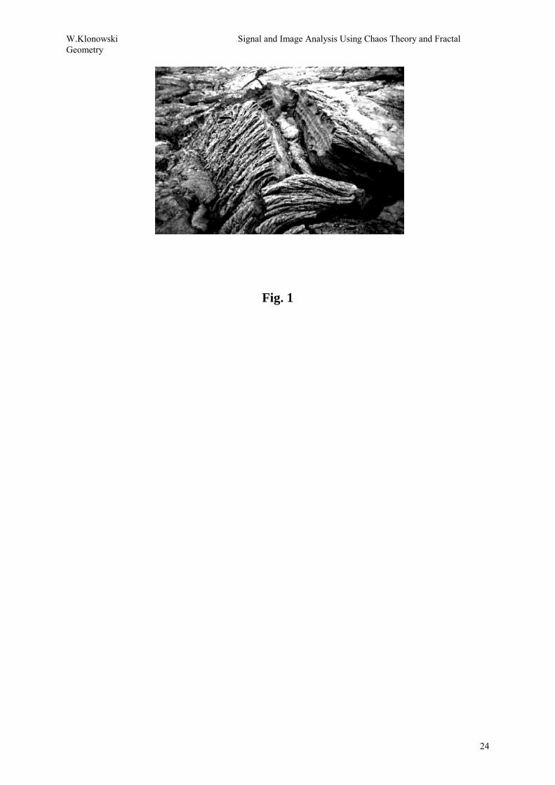
W.Klonowski Signal and Image Analysis Using Chaos Theory and Fractal Geometry
24
Fig. 1
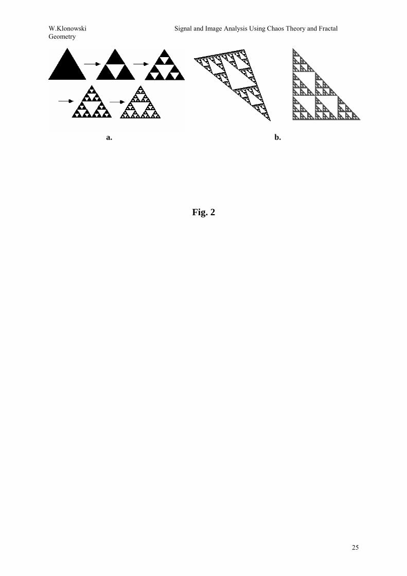
W.Klonowski Signal and Image Analysis Using Chaos Theory and Fractal Geometry
25
a. b.
Fig. 2

W.Klonowski Signal and Image Analysis Using Chaos Theory and Fractal Geometry
26
a. b.
Fig. 3 and Fig. 4
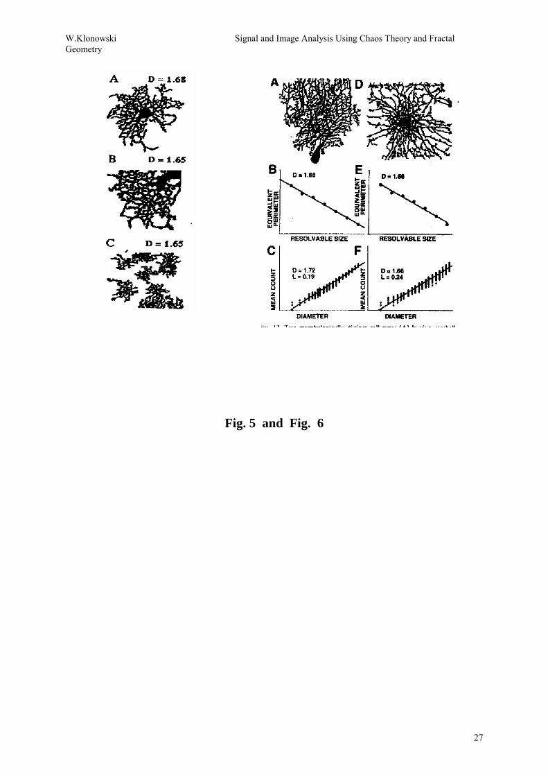
W.Klonowski Signal and Image Analysis Using Chaos Theory and Fractal Geometry
27
Fig. 5 and Fig. 6
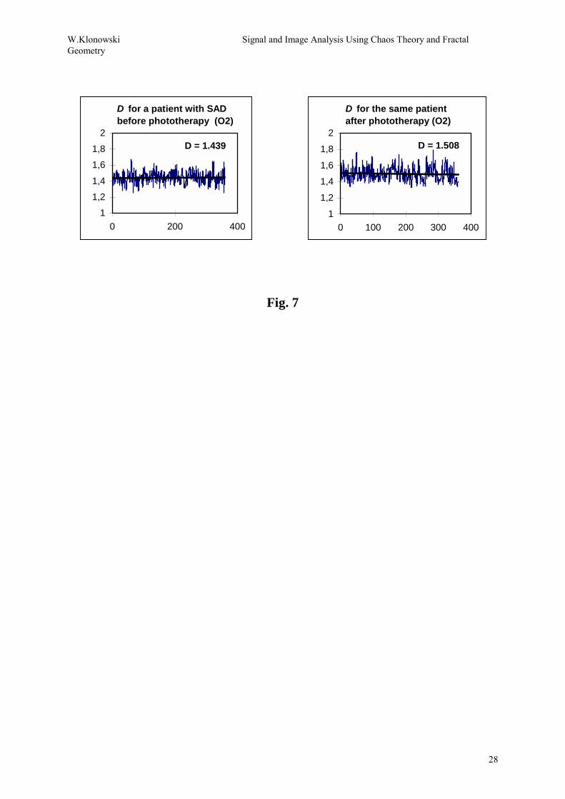
W.Klonowski Signal and Image Analysis Using Chaos Theory and Fractal Geometry
28
Fig. 7
D for the same patientafter phototherapy (O2)
D = 1.508
1
1,2
1,4
1,6
1,8
2
0 100 200 300 400
D for a patient with SAD before phototherapy (O2)
D = 1.439
11,21,4
1,61,8
2
0 200 400

29
Fig. 8 and Fig. 9
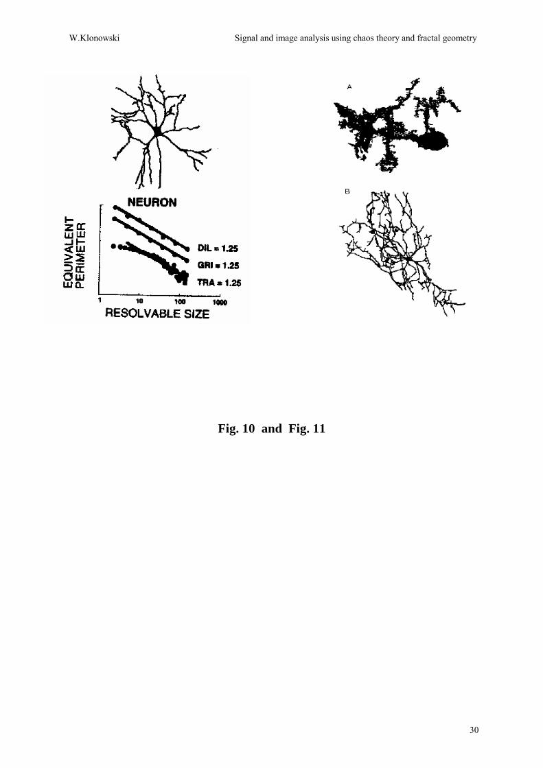
W.Klonowski Signal and image analysis using chaos theory and fractal geometry
30
Fig. 10 and Fig. 11
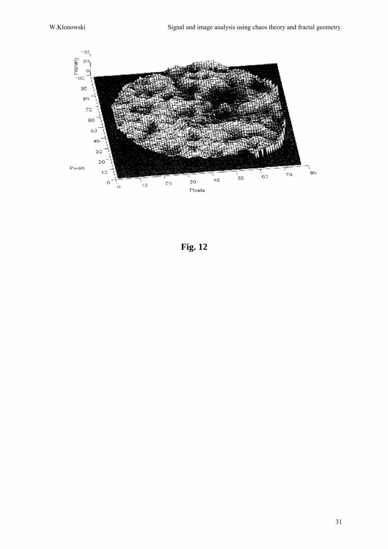
W.Klonowski Signal and image analysis using chaos theory and fractal geometry
31
Fig. 12

Filename: GKPO2000gr Directory: F:\Web\tobinary Template: C:\Program Files\Microsoft Office\Office\Normal.dot Title: SIGNAL AND PATTERN ANALYSIS USING CHAOS
THEORY AND FRACTAL GEOMETRY Subject: Author: W.Klonowski Keywords: Comments: Creation Date: 2000-12-19 22:40 Change Number: 3 Last Saved On: 2000-12-19 22:45 Last Saved By: W.Klonowski Total Editing Time: 13 Minutes Last Printed On: 2001-01-26 12:38 As of Last Complete Printing Number of Pages: 31 Number of Words: 11 338 (approx.) Number of Characters: 64 627 (approx.)