SIGGRAPH Course 2014 — Skinning: Real-time Shape DeformationPart III: Example-based Shape Deformation v1.01

J.P. Lewis

Victoria University and Weta Digital

1 Introduction

Example-based skinning approaches generate skinning and other effects by interpolating a set of sculpted or scanned examples of thedesired deformation, where the interpolation happens in a “pose space” defined by the joint angles and other degrees of freedom ofthe creature rig.

The example-based approaches are distinguished by two main ideas:

1. Skinning usually specifies the deformed position of a vertex using a short algorithm, such as linear blend skinning or dualquaternion skinning. In contrast, example based approaches interpolate a set of examples of the desired deformation.

2. Traditionally animation has been abstractly considered as a function of time, i.e.

shape = f(time)

In computer graphics we are also familiar with surface interpolation, where

shape = f(space).

In contrast, example-based approaches considershape = f(pose)

where “pose” is the pose of the underlying skeleton (usually) or other non-spatial parameters.

The example-based skinning (EBS) approach has evident advantages and disadvantages:

• The desired deformation is directly sculpted, so the artist gets exactly what s/he wants. Algorithmic skinning approachesgenerally require specifying parameters that only indirectly relate to the desired shape, such as the weights on varioustransforms.

• The range of possible deformed shapes is much larger than is achievable with current algorithmic skinning algorithms. Forexample, it is possible to sculpt a shape that includes a bulging muscle and extruding veins. The example-based approachpermits a progressive refinement strategy, whereby additional shapes are added as needed to obtain the desired quality.

• Among disadvantages of EBS, it requires considering higher-dimensional pose spaces. For example, the number of rotationsinfluencing the shoulder region is probably more than three, and the number of bones influencing the neck/trunk area of ananimal such as an elephant might be 10 or more. EBS requires computation proportional to the number of examples. This islikely higher than the amount of computation required for algorithmic skinning.

• Lastly, EBS can require some awareness of the numerical considerations that arise in interpolation and data fitting. Theseinclude regularization and the curse of dimensionality.

Example-based and algorithmic skinning approaches are not mutually exclusive however. On the contrary, example-based skinningis usually implemented as a correction on top of algorithmic skinning.

The deformed postion of a single vertex v′ at a pose p will be interpolated from the corresponding positions specified at exampleposes pk. Preferably, an EBS system should allow the artist to specify a desired shape at any location in the pose space as desired(Figure 1). Since these locations have no regularity, this requires the use of a scattered interpolation algorithm.

This section of the course will first describe some of the example-based algorithms, while leaving the underlying scatteredinterpolation method as an unspecified “black box”. Next, several examples and appplications of EBS methods will be mentioned.Following that, we will review scattered interpolation methods that have been used for EBS. Lastly, numerical considerations will bementioned. Skinning is a core component of the broader subject of “rigging”. For recent surveys of character and facial rigging, see[McLaughlin et al. 2011; Orvalho et al. 2012].

SIGGRAPH Course 2014 — Skinning: Real-time Shape DeformationPart III: Example-based Shape Deformation v1.01 J.P. Lewis

Figure 1: Scattered interpolation of a creature’s skin as a function of skeletal pose. Left, A point on the forearm (red in the electronicversion) moves as a function of two degrees of freedom (dofs): the elbow rotation and the forearm twist. Example shapes describingthe deformation of this point are interpolated in an abstract 2-dof pose space (right).

2 EBS Algorthms

2.1 Pose Space Deformation

In the pose-space deformation (PSD) algorithm [Lewis et al. 2000], the artist moves the underlying skeleton to particular poses andsculpts examples of the desired shape at those poses. The sculpts are saved and associated with the corresponding pose. The PSDsystem interpolates these examples as a function of pose.

The pose space is a set of degrees of freedom of the rig that vary between the example shapes, and a particular pose is a set ofparticular values of these degrees of freedom (not to be confused with the shape that the model has at that pose). Typically, the posespace is the set of joint angles of the skeleton that vary across the given shapes. If the sculpted examples are of the shoulder region,the “pose space” would consist of the joint rotations of the bones that plausibly affect the shoulder. More generally, however, thepose space can include other attributes. For example it might include a degree of freedom describing “exertion”, so that muscles canbulge appropriately when the body is carrying weight. [Sloan et al. 2001a] termed these degrees of freedom “adjectives.”

The interpolation of the examples has the pose space as its domain, and 3D space is the range of the interpolation. For example, apoint near the neck may be affected by three bones. A joint between two such bones might be described by two relative angles. Thethree-bone configuration has two internal joints, so the pose space in this case has four dimensions. The interpolation is then from a4-dimensional pose space to 3D (geometry) space (<4 → <3).

Since the examples can be created at arbitrary locations, this is a scattered interpolation problem (Figure 1). In machine learningterms it can also be considered as an instance of non-parametric regression (“non-parametric” refers to a model whose complexityincreases with the available data, as opposed to a parametric model such as a Gaussian that has a fixed number of parameters(e.g. mean, variance) regardless of the amount of data). In the machine learning terminology the collected set of example shapes maybe termed “training” shapes.

The example based approach is extremely simple (although it can be occasionally confusing to mentally switch between thinkingabout 3D space and the higher-dimensional pose space!) EBS algorithms differ in the way they handle several specific issues,described next:

2 of 20

SIGGRAPH Course 2014 — Skinning: Real-time Shape DeformationPart III: Example-based Shape Deformation v1.01 J.P. Lewis

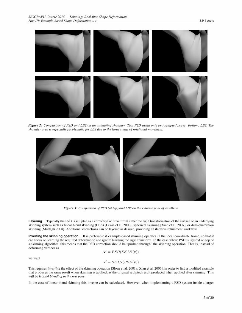
Figure 2: Comparison of PSD and LBS on an animating shoulder. Top, PSD using only two sculpted poses. Bottom, LBS. Theshoulder area is especially problematic for LBS due to the large range of rotational movement.

Figure 3: Comparison of PSD (at left) and LBS on the extreme pose of an elbow.

Layering. Typically the PSD is sculpted as a correction or offset from either the rigid transformation of the surface or an underlyingskinning system such as linear blend skinning (LBS) [Lewis et al. 2000], spherical skinning [Xian et al. 2007], or dual-quaternionskinning [Murtagh 2008]. Additional corrections can be layered as desired, providing an iterative refinement workflow.

Inverting the skinning operation. It is preferable if example-based skinning operates in the local coordinate frame, so that itcan focus on learning the required deformation and ignore learning the rigid transform. In the case where PSD is layered on top ofa skinning algorithm, this means that the PSD correction should be “pushed through” the skinning operation. That is, instead ofdeforming vertices as

v′ = PSD(SKIN(v))

we wantv′ = SKIN(PSD(v))

This requires inverting the effect of the skinning operation [Sloan et al. 2001a; Xian et al. 2006], in order to find a modified examplethat produces the same result when skinning is applied, as the original sculpted result produced when applied after skinning. Thiswill be termed blending in the rest pose.

In the case of linear blend skinning this inverse can be calculated. However, when implementing a PSD system inside a larger

3 of 20

SIGGRAPH Course 2014 — Skinning: Real-time Shape DeformationPart III: Example-based Shape Deformation v1.01 J.P. Lewis

package such as Maya, the existing skinning and rigging operations may be more complicated algorithms or proprietary “black box”deformers. In these production situations [Xian et al. 2006] proposed the use of derivative-free optimization to invert an arbitraryexisting skinning rig.

The following three issues are distinct but related:

• Per-shape or per-vertex interpolation.

Shape-by-example [Sloan et al. 2001a] used cardinal interpolation of the examples, with the same weights applied to allvertices of the example meshes (the blending is done in the rest pose space). Other methods have used differing interpolationat each vertex – this is required in the case of weighted pose space deformation.

• Local or global interpolation in the pose space.

All the degrees of freedom of the model can be concatenated to form a single global pose space. This presents problemshowever: consider a point on the fore-arm, as in Figure 1. If the pose space also contains the dofs of the legs, then movingthe legs will affect the relative distance of the current pose from the poses that involve arm motion. In concept this could beaddressed by adding examples with the legs in all possible shapes for every desired shape of the arm.

This is an instance of the “curse of dimensionality” – the needed amount of training data rises exponentially with increasingdimension. The original PSD algorithm avoided the problem by using separate per-vertex interpolation, relying on splineinterpolation to avoid any discontinuities. The weighted pose space deformation algorithm introduced a better approach, inwhich irrelevant dofs are smoothly attenuated (according to the underlying skinning weights) when calculating the distancein pose space. This results in a collection of smoothly coupled local regression problems, thereby addressing the curse ofdimensionality without introducing discontinuities.

• Interpolation algorithm.

Independent of whether the interpolation is per-vertex or per-shape, or local or global in the pose space, different scatteredinterpolation algorithms can be chosen. Approaches that have been employed include linear interpolation, natural neighborinterpolation, and radial basis interpolation with several types of kernels. These possibilities are reviewed in section 4.

2.2 Shape by Example

Shape-by-Example is a technique presented by Sloan, Rose, and Cohen at the 2001 I3D conference [Sloan et al. 2001a]. Theirtechnique has some broad similarities to PSD. It differs in that the interpolation is formulated as a cardinal interpolation of theexamples in the pose space.

In this scheme, for n example shapes there are n separate interpolators, with the kth interpolator using data that is 1 at the k trainingpose and 0 at all the other poses. These are then simply used as weights in a shape interpolation, albeit one that happens in the restpose as described above.

The use of cardinal interpolation has several advantages. It uses a single global pose space for all examples, which is easier to thinkabout. It also provides considerable efficiency if separate per-vertex interpolation effects are not required.

Another innovation in this work was the concept of pseudo-examples. In this approach, the artist finds an acceptable interpolatedshape situated at the wrong location in the abstract pose space. Rather than sculpt new examples, the interpolated shape is simplymoved to a new location in the pose space. The result is that the pose space itself is reshaped. This can be desirable if, for example, aparticular interpolation begins and ends with the right shape, but interpolates too quickly or slowly.

2.3 Weighted Pose Space Deformation

Kurihara and Miyata [Kurihara and Miyata 2004] introduced the weighted pose-space deformation (WPSD) algorithm. The WPSDalgorithm solves the curse of dimensionality to some extent. It greatly reduces the number of training examples required, particularlyfor complex regions such as the hand that may have as many as 40 parameters or more. This is accomplished by formulating theinterpolation as a set of separate but softly-coupled interpolations, one per vertex. The skinning weights are used to determine aper-vertex distance between poses,

dj(pa,pb) =

√√√√ n∑k

wj,k(pa,k − pb,k)2

where wj,k are the skinning weights for the kth degree of freedom for the jth vertex, and pa,k denotes the kth component of locationpa in the pose space.

The example shapes in [Kurihara and Miyata 2004] were captured using a medical scan of one of the authors’ hands, resulting invery plausible and detailed shapes (Fig. 4). The video accompanying the paper shows that the interpolation of these shapes as thefingers move is also very realistic.

4 of 20

SIGGRAPH Course 2014 — Skinning: Real-time Shape DeformationPart III: Example-based Shape Deformation v1.01 J.P. Lewis

Figure 4: Hand poses synthesized using weighted pose space deformation (image from [Kurihara and Miyata 2004] ©TsuneyaKurihara).

Kurihara and Miyata used the cardinal interpolation scheme from [Sloan et al. 2001b], in combination with normalized radial basisfunctions. The RBF matrix is based on the distance between the poses (in pose space) and so has to be formed and inverted onlyonce.

2.4 Context-Aware Skeletal Shape Deformation

[Weber et al. 2007] might be summarized as being a combination of deformation transfer [Sumner and Popovic 2004] and weightedpose space deformation [Kurihara and Miyata 2004]. WPSD is used to blend triangles of the examples in the rest space. Thesetriangles are then transformed by the skeleton’s rigid motion using a approach inspired by deformation transfer. Specifically, thevarious bone transform affecting a particular triangle are blended (with log-quaternion blending of the joint rotations). The finalposition of each triangle is obtained by solving a Poisson problem involving the deformation gradient (Jacobian) of each triangle[Botsch et al. 2006]. In an initial step the skinning weights are computed automatically using a harmonic cardinal interpolation ofregions that are marked by the artist as moving rigidly with particular joints.

2.5 Other Algorithms

A future version of this document may cover other example-based skinning algorithms including [Kry et al. 2002; Bickel et al.2008].

3 EBS Applications

3.1 Skeleton-Driven Deformation

An articulated model such as a human will typically have a number of different deformation subspaces, each with one or severaldeformations; the deformations in different subspaces may overlap spatially e.g. to simulate the influence of different muscles. Thedeformations needed for an elbow, for example, will be interpolated in the one-dimensional subspace defined by the elbow jointangle. Deformations in a shoulder area will need to consider two or more degrees of freedom. The neck/chest/leg blend area of manyquadrupeds is a more complex case – the motion of the skin surface in these regions may depend on the relative configuration ofseveral leg bones as well as the rib cage and possibly the neck region of the spine. The example-based approach handles all thesecases simply and uniformly.

Figure 2 and 3 show PSD and LBS algorithms in action on human elbow and shoulder regions.

3.2 Secondary Animation

Additional “dimensions” of deformation can be created by adding a new parameter and associating additional poses with themovement of this parameter. For example, a limb can be modeled in a particular pose both in an unloaded state and with musclessculpted to express carrying a heavy load. The ‘heavy’ pose can be associated with the ‘on’ state of an abstract parameter; light andheavy loads can then be controlled by flipping this switch.

5 of 20

SIGGRAPH Course 2014 — Skinning: Real-time Shape DeformationPart III: Example-based Shape Deformation v1.01 J.P. Lewis

w3

w1

w2

Figure 5: The delta blendshape scheme can be visualized as situating targets at vertices of a hypercube that share an edge with theneutral face at the origin.

Figure 6: Blendshape schemes require that targets are placed at constrained locations, i.e. the vertices of a “weight hypercube”(Fig. 5). Example-based approaches allow targets to be placed anywhere in facial expression space, allowing the sculpting effort tobe directed specifically where it is needed.

Figure 7: Schematic diagram of emotion space obtained by multi-dimensional scaling from pairwise similarity ratings, simplifiedfrom [Russell 1980].

3.3 Using PSD to “Reparameterize” an Existing Rig

PSD can also be used to control parameters of a lower level “rig”, rather than directly controlling geometry. It has often beenemployed this way in practice [Lee and Hanner 2009; Komorowski et al. 2010].

In this approach, the artist invents a new space for interpolation, with associated parameters that serve as controls. The underlyinginterpolation maps these visible parameters to the parameters of the underlying system, which are typically lower level or lessconvenient. The desired control scheme is specified simply by providing examples of the desired mapping.

3.4 Facial Animation

Disney introduced the use of PSD for facial animation [Lee and Hanner 2009; Komorowski et al. 2010] (also [Lee 2009]).

6 of 20

SIGGRAPH Course 2014 — Skinning: Real-time Shape DeformationPart III: Example-based Shape Deformation v1.01 J.P. Lewis

Figure 8: Smoothly propagating an expression change to nearby expressions using Weighted Pose Space Editing [Seol et al. 2012].

Decoupling parameters from examples. An advantage of example-based approaches for facial animation is that it decouples thecontrol parameters from the location of the examples. In blendshape animation, each blendshape target defines a control parameter.Abstractly, the examples (targets) are situated at some of the vertices of a hypercube (Figure 5). In an example-based approach, theartist defines a set of control parameters as desired, and then can place the example shapes anywhere in the space defined by theseparameters (Figure 6). The number of example shapes does not need to be the same as the number of parameters.

As a simple example, one could take an emotion space identified in psychological research as the pose space. [Russell 1980]performed multidimensional scaling (MDS) on surveys of pairwise similarity ratings between various facial expressions involvingemotion, and identified two axes that can be interpreted as happy-sad and low-high energy. In this space, for example, “content” islow-energy but happy, whereas “bored” is low-energy but less happy. An emotional face model could be constructed by sculpting anynumber of facial expressions representing various emotions, and then placing them at the appropriate point in the space (Figure 7).

This simple example shows how using a pose space can greatly reduce the number of parameters that the artist needs to control. Onthe other hand, expressive facial animation is a high-dimensional problem even if the most economical parameterization is used.For this reason, an example-based approach that directly controls the facial geometry should make use of the coupled local modelsintroduced by the WPSD scheme [Kurihara and Miyata 2004].

A hybrid approach. Blendshapes are based on simple linear interpolation, which leaves much to be desired, particularly whenseveral shapes are combined. One solution involves adding a number of correction shapes [Osipa 2007; Seo et al. 2011]. Each suchshape is a correction to a pair (or triple, quadruple) of primary shapes. While this improves the interpolation, it is an expensivesolution due to the number of possible combination shapes. Finding the correct shapes also involves a labor-intensive trial anderror process. Typically a bad shape combination may be visible at some arbitrary set of weights such as (w10 = 0.3, w47 = 0.65).The blendshape correction scheme does not allow a correction to be associated with this location, however, so the artist must findcorrections at locations (vertices of the weight hypercube) such as (w10 = 1, w47 = .1), (w10 = 1, w47 = 0), (w10 = 0, w47 = 1)that together add to produced the desired shape. This requires iterative resculpting of the relevant shapes.

To solve this problem, Seol et al. [Seol et al. 2012] combine ideas from blendshapes and weighted pose space deformation.Specifically, they use an elementary blendshape model (without corrections) as both a base model and a pose space for interpolation.Then, the weighted PSD idea is used to interpolate additional sculpted shapes. These shapes can be situated at any location in theweight space, and they smoothly appear and fade away as the location is approached (Figure 8). Because of the unconstrainedlocation of these targets and the improved interpolation, both the number of shapes and the number of trial-and-error sculptingiterations are reduced.

7 of 20

SIGGRAPH Course 2014 — Skinning: Real-time Shape DeformationPart III: Example-based Shape Deformation v1.01 J.P. Lewis

3.5 Clothing

Example-based methods have been employed to generate the deformation of clothing. [Zurdo et al. 2013] used WPSD to adddynamic wrinkle detail to a low-resolution cloth model.

4 Deformation as Scattered Interpolation

Figure 9: Shepard’s interpolation with p = 2. Note the the derivative of the function is zero at the data points, resulting in smoothbut uneven interpolation. This same set of points will be tested with the RBF interpolation methods discussed below.

0 50 100 150 2000

2

4

6

8

10

12

14

Figure 10: Shepard’s interpolation with p = 1.

In abstract, we wish to express the deformation of a surface as a function of either the pose of an underlying skeleton, or equivalentlyas a function of some other set of parameters such as the {smile, raise-eyebrow,...} controls desirable in facial animation. We alsowish to directly sculpt the desired deformation at various points in the pose space, rather than working in a more abstract space suchas the coefficients on various transforms as required by the LBS algorithm.

A scattered data interpolation method is required because deformations will be sculpted at arbitrary (rather than regularly spaced)poses. Since this interpolation is central to our application (the results of the interpolation will be directly visible as the animatingdeformation), we will consider the available scattered interpolation approaches.

In theory an example-based skinning algorithm such as PSD can be implemented using any scattered interpolation scheme. Forexample the author is aware of one implementation based on natural neighbor interpolation [Sibson 1981],

4.1 Linear Interpolation

Because high-dimensional functions are difficult to visualize and control, [Bengio and Goldenthal 2013] introduced a variant ofpose space deformation that uses simple linear interpolation on the data simplices. ([Lee 2009] may have also used this idea,though it is difficult to say from the one-page description). This approach sacrifices smoothness but prevents overshoot; this was therecommendation in the evaluation [Lee 2009].

8 of 20

SIGGRAPH Course 2014 — Skinning: Real-time Shape DeformationPart III: Example-based Shape Deformation v1.01 J.P. Lewis

Implementing linear interpolation requires first “triangulating” the domain of example poses into a set of simplices. A simplex is then-dimensional generalizations of a triangle: a triangle is 3 points in two dimensions, a tetrahedron is 4 points in three dimensions,and a general simplex is d+1 points in d dimensions. Each “point” is a location in the pose space, with an associated geometric poseof the creature. Computational geometry libraries such as qdelaunay can be used for this purpose [Bengio and Goldenthal 2013].After the simplices are obtained, interpolation can be performed using the d-dimensional generalization of barycentric interpolation.Specifically, the weights on the vertices of a simplex can be found by solving a block linear system[

P1

] [w]=

[p1

]Here P is a d× d+ 1 matrix whose columns contain the locations of the vertices of the simplex, so the upper equation Pw = p isexpressing a particular location p as a weighted sum of the vertices. 1 is a row vector of ones, so the bottom row 1Tw = 1 requiresthat the sum of the weights be one. If all the weights are non-negative the location p is inside the simplex. Then, the geometry at thislocation can be obtained as a weighted sum of the geometry associated with each vertex of the simplex, using w as the weights. Ifany of the weights are below zero, then the particular point p is outside of this simplex, and other simplices should be tested.

In addition to lack of smoothness, linear interpolation is impractical in high dimensions because the number of simplices adjacent toa particular vertex grows factorially with the dimension.

4.2 Splines with Tension

0 50 100 150 2001

2

3

4

5

6

7

0 50 100 150 2001.5

2.0

2.5

3.0

3.5

4.0

4.5

5.0

5.5

6.0

Figure 11: Spline with tension. Left, cubic spline interpolation. Right, cubic spline interpolation of the same points, with tension.The boundary conditions are set to have zero slope (Dirichlet).

The tradeoff between smoothness and overshoot is a fundamental issue in interpolation. Using linear interpolation is not the onlyway to control overshoots. Splines with “tension” result from minimizing an objective that includes a weighted sum of the squaredfirst and higher order derivatives, integrated over the function (Equation (2)). The weights provide a “knob” that allows the amountof smoothness to be controlled. Splines with tension can in theory be implemented through radial basis interpolation (section 1),although the RBF kernel function for this purpose has not been worked out in higher dimensions. Shepard’s method (Section 4.3)can produce an interpolated function whose derivative is zero at the gradients. This may be considered as an artifact, or an advantage,since it has the effect of reducing overshoot.

4.3 Shepard’s Method

Shepard’s method [Barnhill et al. 1983; Beier 1992] is a frequently employed scattered data interpolation scheme in computergraphics. In this method the interpolated value is a weighted sum of the surrounding data points normalized by the sum of theweights,

d(p) =

∑wk(p)dk∑wk(p)

with weights set to an inverse power of the distance: wk(p) = ‖p − pk‖−p. (This is singular at the data points pk andshould computed as (||p − pk‖ + ε)−p). With p > 1 the interpolated function is once differentiable. Unfortunately thissimple scheme has some potentially undesirable properties. Far from the data the weights will be approximately the same,d(∞) = w∞

∑dk/w∞

∑1 =

∑dk/N , i.e. the interpolated surface converges to the average of the data values. A serious

drawback for some applications is that the derivative of the surface is zero at the data points (Figure 4).

9 of 20

SIGGRAPH Course 2014 — Skinning: Real-time Shape DeformationPart III: Example-based Shape Deformation v1.01 J.P. Lewis

Figure 12: Schematic illustration of RBF interpolation in one dimension. A fixed-width kernel is situated at each data point (coloredcurves). The weighted sum of these interpolates the given data (dashed line). The weights are obtained by solving a linear system.

This problem can be addressed by using moving least squares schemes [Cheng et al. 2008; Lancaster and Salkauskas 1986]. Theseinvolve fitting a low-order polynomial over a sliding window of nearby points, using a weighted least squares scheme to reduce theinfluence of points at the edge of the neighborhood. While moving least squares could be used to implement pose space deformation,the training example poses may have very uneven distribution in the pose space, thus making the notion of “neighborhood” fragile.Radial basis functions (described below) are an alternate choice.

4.4 Radial Basis Functions

Radial basis functions [Powell 1990; Powell 1987] have become a popular choice for scattered interpolation. The interpolant is alinear combination of nonlinear functions of distance from the data points (Figure 12):

d(p) =

N∑k

wkR(‖p− pk‖) (1)

If N values of d are available then the weights can be easily solved by a linear system of the formR1,1 R1,2 R1,3 · · ·R2,1 R2,2 · · ·R3,1 · · ·

...

w1

w2

w3

...

=

d1d2d3...

(compactly, Rw = d) where Ri,j denotes R(‖pi − pk‖) and di are the data points to interpolate, giving the solution1

w = R−1d

The distance ‖‖ can be generalized to Mahalanobis distance (effectively rotating and stretching the basis function) [Bishop 1995].

4.4.1 What is the right RBF kernel?

Different choices of the RBF kernel function R are possible. Kernels corresponding to n-harmonic splines are discussed in Section 5.The choice involves the definition of smoothness and the tradeoff between smoothness and overshoot.

The Gaussian kernel involves a width parameter σ, as do some other kernels. It is possible to choose this width parameter to locallyadapt to the data, so that kernels centered at different locations have different widths [Bishop 1995], however the resulting problem isnot convex, and a more expensive nonlinear optimization would be required.

A practical recommendation is to use normalized radial basis functions in combination with cardinal interpolation, as is done inWPSD. Normalized radial basis functions are somewhat less sensitive to the choice of kernel width. Cardinal interpolation has adata-adaptive effect by forcing the interpolated function to zero at the locations of other training examples.

1The paper [Lewis et al. 2000] described a geometric derivation, in which the available data points are considered as a single point d in an Ndimensional space. The best approximation to d in the space spanned by R occurs (in direct analogy with the three-dimensional case) when theweights are such that the error d−Rw is orthogonal to each column of R:

RT (Rw − d) = 0

giving the normal equation formRTRw = RTd

that can be solved forw = (RTR)−1RTd

The normal equations form generalizes to the case where there are fewer RBF kernels than data points, as arises with some model simplificationschemes. However in the simple case where an RBF kernel is centered at each data point, the normal equations form provides no advantage and onthe contrary has a poorer condition number due to the squaring of the R matrix.

10 of 20

SIGGRAPH Course 2014 — Skinning: Real-time Shape DeformationPart III: Example-based Shape Deformation v1.01 J.P. Lewis

0 50 100 150 2000

2

4

6

8

10

12

14

Figure 13: One-dimensional radial basis interpolation with a Gaussian kernel. The curve extrapolates to zero.

0 50 100 150 2000

2

4

6

8

10

12

14

Figure 14: Radial basis interpolation with a Gaussian kernel, varying the kernel width relative to Fig. 13

0 50 100 150 2000

2

4

6

8

10

12

14

Figure 15: Radial basis interpolation with a Gaussian kernel, varying the kernel width relative to Fig. 13,14. In this figure the kernelwidth is too narrow to adequately interpolate the data.

4.5 Interpolation of 3D Data

The preceding description maps a k-dimensional input space (arbitrary k) to a one dimensional range, i.e., it is the k-dimensionalversion of a height field. Three-dimensional data can be interpolated by using three separate one-dimensional interpolations, one eachfor x, y, z. In the case of radial basis function interpolation, the R matrix is common to the three dimensions and can be inverted justonce.

11 of 20

SIGGRAPH Course 2014 — Skinning: Real-time Shape DeformationPart III: Example-based Shape Deformation v1.01 J.P. Lewis

5 Numerical Considerations

0 50 100 150 2000

2

4

6

8

10

12

14

Figure 16: The one-dimensional equivalent of thin-plate spline interpolation is the natural cubic spline, with radial kernel |r|3 inone dimension. This spline minimizes the integrated square of the second derivative (an approximate curvature) and so extrapolatesto infinity away from the data. !1 !0.5 0 0.5 1

!1

0

10

0.5

1

!1 !0.5 0 0.5 1!1

0

10

0.5

1

!1 !0.5 0 0.5 1

!0.2

!0.1

0

0.1

0.2

0.3

0.4

0.5

Figure 17: Comparison of the 3D biharmonic clamped plate spline (black line) with Gaussian RBF interpolation (red) [Rhee et al.2011].

A variety of functions can be used as the radial basis kernel R(r). Some of the most common choices in the literature are(c.f. [Fasshauer 2007, Appendix D]):

Gaussian R(r) = exp(−(r/c)2)Hardy multiquadric R(r) =

√r2 + c2

Inverse multiquadric R(r) = 1/√r2 + c2

Thin plate spline R(r) = r2 log r (in two dimensions)

Laplacian (or Polyharmonic) splines R(r) ∝

{r2s−n log r if 2s− n is an even integer,r2s−n otherwise

In fact there is not yet a general characterization of what functions are suitable as RBF kernels [Fasshauer 2007]. Positive definitefunctions are among those that will generate a non-singular R matrix for any choice of data locations. There are several alternatecharacterizations of positive definiteness:

• A function is positive definite if ∑i

∑k

wiwkR(‖xi − xj‖) > 0

for any choice of unique data locations xi.

• A positive definite function is a Fourier transform of a non-negative function [Lewis 1987]. (Note that “positive definite” doesnot mean that the function itself is necessarily positive. The sinc function is a counter example, since it is the transform of abox function.)

• The matrix R generated from a positive-definite kernel function has all eigenvalues positive.

The third characterization indicates that for a positive definite function, the matrix R will be invertable for any choice of data points.On the other hand, there are useful kernels (such as the polyharmonic family) that are not positive definite.

Several aspects of radial basis kernels are not intuitive at first exposure. The polyharmonic and thin-plate kernels are zero at the datapoints and increase in magnitude away from the origin. Also, kernels that are not themselves smooth can combine to give smoothinterpolation. An example is the second-order polyharmonic spline in 3 dimensions, with kernel R(r) = |r|.

12 of 20

SIGGRAPH Course 2014 — Skinning: Real-time Shape DeformationPart III: Example-based Shape Deformation v1.01 J.P. Lewis

Several of the common RBF kernels have an explicit width parameter (e.g. the Gaussian σ). The use of a broad kernel can causesurprising effects. This is due to the near-singularity of the R matrix resulting from rows that are similar. The problem (and asolution) is discussed in section 5.1.

When thinking about the appropriate kernel choice for an application, it is also worth keeping in mind that there is more than oneconcept of smoothness. One criterion is that a function has a number of continuous derivatives. By this criterion the Gaussianfunction is a very smooth function, having an infinite number of derivatives. A second criterion is that the total curvature should besmall. This can be approximated in practice by requiring that the solution should have a small integral of squared second derivatives –the criterion used in the thin-plate and biharmonic splines.

This second criterion may correspond better to our visual sense of smoothness, see Figures 16, 17. Figure 16 shows a natural cubicspline on scattered data points. The curve extrapolates beyond the data, rather than falling back to zero, which may be an advantageor disadvantage depending on the application. Figure 17 compares two approaches that both fall to zero: Gaussian RBF interpolation(red) and the 3D biharmonic clamped plate spline (black line). The plot is the density of a linear section through an interpolatedvolume. Note that the control points are distributed through the volume and cannot meaningfully be visualized on this plot. Althoughthe Gaussian function has an infinite number of derivatives, Gaussian RBF interpolation is visually less smooth than the biharmonicspline. The visual smoothness of the Gaussian can be increased by using a broader kernel, but this also increases the overshoots.

For many applications the most important considerations will be the smoothness of the interpolated function, whether it overshoots,and whether the function decays to zero away from the data. For example, artists tend to pick examples at the extrema of the desiredfunction, so overshoot is not desirable. As another example, in the case where a pose space deformation algorithm is layered on topof an underlying skinning algorithm, it is important that the interpolated function fall back to zero where there is no data.

Of course it is not possible to simultaneously obtain smoothness and lack of overshoot, nor smoothness and decay to zero away fromthe data. It is possible, however, to combine these criteria with desired strengths. The approach is to find the Green’s function (seesection 5.6) for an objective such as

F (f) =∑

(f(xi)− yi)2 + α

∫‖∇2f‖2dx

+ β

∫‖∇f‖2dx

+ γ

∫‖f‖2dx

(2)

i.e. a weighted sum of the data fidelity and the integral of the squared second derivative, the squared first derivative (i.e. “spline withtension”), and the squared function itself (causing the function to decay to zero).

The kernel choice leads to numerical considerations. The Gaussian kernel can be approximated with a function that falls exactly tozero resulting in a sparser and numerically better conditioned matrix matrix [Wendland 2009], while the polyharmonic kernels areboth dense and ill-conditioned.

5.1 Regularization

0 50 100 150 2000

2

4

6

8

10

12

14

Figure 18: Adding regularization to the plot in Fig. 16 causes the curve to approximate rather than interpolate the data.

In creating training poses for example-based skinning, the artist may accidentally save several sculpted shapes at the same pose. Thisresults in a singular R matrix. This situation can be detected and resolved by searching for identical poses in the training data.

A more difficult case arises when there are several (hopefully similar) shapes at placed at nearly but not exactly the same location inthe pose space. In this case the R matrix is not singular, but is poorly conditioned. The RBF result will probably pass through the

13 of 20

SIGGRAPH Course 2014 — Skinning: Real-time Shape DeformationPart III: Example-based Shape Deformation v1.01 J.P. Lewis

0 1 2 3 4 52

1

0

1

2

3

4

5

0 1 2 3 4 51.5

1.0

0.5

0.0

0.5

1.0

1.5

Figure 19: One-dimensional values interpolated with a Gaussian kernel that is too broad for the data spacing, resulting in badconditioning. Left, no regularization. Right, regularization parameter 0.00001

�2.0 �1.5 �1.0 �0.5 0.0 0.5 1.0 1.5 2.0�1.2

�1.0

�0.8

�0.6

�0.4

�0.2

0.0

0.2

�2.0 �1.5 �1.0 �0.5 0.0 0.5 1.0 1.5 2.0�0.04

�0.03

�0.02

�0.01

0.00

0.01

0.02

0.03

�2.0 �1.5 �1.0 �0.5 0.0 0.5 1.0 1.5 2.0�0.005

0.000

0.005

0.010

0.015

0.020

0.025

Figure 20: Illustration of ill-conditioning and regularization in a 3D example. From left to right, the regularization parameter is 0,.01, and .1 respectively. Note the vertical scale on the plots is changing. Bottom: The geometry of this 3D interpolation problem.The data are zero at the corners of a square, with a single non-zero value in the center. The plots show a single section through theinteroplated function.

given datapoints, but it may do wild things elsewhere (Figure 20). Intuitively speaking, the matrix is dividing by “nearly zero” insome directions, resulting in large overshoots.

In this case an easy fix is to apply weight-decay regularization. Rather than requiring Rw = d exactly, weight-decay regularizationsolves

argminw‖Rw − d‖2 + λ‖w‖2 (3)

This adds a second term that tries to keep the sum-square of the weight vector small. However, λ is chosen as a very small adjustablenumber such as 0.00001. In “directions” where the fit is unambiguous, this small number will have little effect. In directions wherethe result is nearly ambiguous however, the λ‖w‖2 will choose a solution where the particular weights are small.

To visualise this, consider a two-dimensional case where one basis vector is pointing nearly opposite to the other (say, at 179 degreesaway). A particular point that is one unit along the first vector can be described almost as accurately as being two units alongthat vector, less one unit along the (nearly) opposite vector. Considering matrix inversion in terms of the eigen decompositionR = UΛUT . of the matrix is also helpful. The linear system is then UΛUTw = d, and the solution is

w = UΛ−1UTd

Geometrically, this is analogous to rotating d by U−1, stretching by the inverse of the eigenvalues, and rotating back. The problematicdirections are those corresponding to small eigenvalues.

14 of 20

SIGGRAPH Course 2014 — Skinning: Real-time Shape DeformationPart III: Example-based Shape Deformation v1.01 J.P. Lewis

Soving (3) for w,

‖Rw − d‖2 + λ‖w‖2

= tr(Rw − d)T (Rw − d) + λwTw

d

dw= 0 = 2RT (Rw − d) + 2λw

RTRw + λw = RTd

giving the solutionw = (RTR + λI)−1RTd

In other words, weight decay regularization requires just adding a small constant to the diagonal of the matrix before inverting.

Fig. 20 shows a section through simple a two-dimensional interpolation problem using a Gaussian RBF kernel. The data are zero atthe corners of a square, with a single non-zero value in the center. Noting the vertical scale on the plots, the subfigures on the leftshow wild oscillation that is not justified by the simple data. In the figures we used weight-decay regularization to achieve a moresensible solution. This also has the effect of causing the reconstructed curve to approximate rather than interpolate the data (Fig. 18).

Weight-decay regularization is not the only type of regularization. Regularization is an important and well studied topic in all areasinvolving fitting a model to data. On a deeper level it is related to model complexity and the bias-variance tradeoff in model fitting.The subject comes up in a number of forms in statistical learning texts such as [Hastie et al. 2009].

5.2 Laplacian Spline and Thin-Plate RBF models

The RBF kernels corresponding to Laplacian splines are augmented with a low order polynomial,

f(x) =

n∑k

ckR(‖x− xk‖) +∑

djpj(x)

with p1(x) = 1 is a constant term. This subsection motivates this alternate formulation.

The RBF and polynomial weights c,d can be solved with a block matrix system[R PPT 0

] [cd

]=

[f0

]where P is the polynomial basis evaluated at all the data points. For example in the 2D thin-plate case a 2D linear polynomial isused, so P is a 3× n matrix containing in its columns the constant function, the x location of each control point, and the y locationof each control point. Note that this matrix is indefinite (has both positive and negative eigenvalues), which rules out the use ofCholeski and conjugate gradient solvers.

Intuitively, the need for a polynomial term arises because these polynomials are in the null space of the differential operator. Forexample, the thin-plate spline minimizes the squared second derivative of the unknown function, integrated over the function. Aconstant or linear term can be added to the function without affecting this functional. Thus, the thin-plate criterion specifies theinterpolation up to a linear polynomial, which must also be estimated. As another example, the criterion of minimizing the integratedsquared gradient is invariant to a constant offset, so the additional polynomial is simply this constant. 2

The additional polynomial coefficients have to be determined somehow. Since the degrees of freedom in the n points are already usedin estimating the RBF coefficients ck, an additional relation must be found. This takes the form of requiring that the interpolationshould exactly reproduce polynomials: If the data f(x) to be interpolated is exactly a polynomial, the polynomial contributioncn+1 · 1 + cn+2 · x + cn+3 · y should be exactly that polynomial, and the weights on the RBF kernel ck, k ≤ n should be zero.

Doing so results in the additional condition that the weights ck are in the null space of the polynomial basis. In showing this we usethe following notation: R is the standard RBF system matrix with the RBF kernel evaluated at the distance between pairs of trainingpoints, c are the RBF weights (coefficients), and f are the desired values to interpolate, so Rc = f would be the system to solve ifthe extra polynomial is not used. Also let P be the polynomial basis, and d be the weights on the polynomial basis. In the 2D casewith a linear polynomial P is a n by 3 matrix with a column of ones, a column of xk, and a column of yk, where (xk, yk) = pk arethe training locations. Then,

2This is related to the fact that the constant function is in the null space of a Laplacian matrix.

15 of 20

SIGGRAPH Course 2014 — Skinning: Real-time Shape DeformationPart III: Example-based Shape Deformation v1.01 J.P. Lewis

Rc + Pd = f the interpolation statementRc + Pd = Pm fit a polynomial Pm, for some unknown coefs m

cTRc + cTPd = cTPm premultiply by cT

cTRc = cTPm− cTPd

cTP(m− d) = cTRc

Then if we require that cTP = 0, then the left hand side is zero, and so c must itself be zero since the right hand side is positive. Sonow going back to the original Rc + Pd = Pm, we know that if cTP = 0, then c = 0, so Rc = 0, so Pd = Pm.

Restating, this means that if the signal is polynomial and we have required cTP = 0, the coefficients c are zero, and then Pd = Pm,so d = m, so the polynomial is exactly reproduced.

Another way of viewing these side conditions is that by imposing an additional relation on c, they reduce the total number of degreesof freedom from n+ p (for a p-order polynomial basis) back to n

The additional relation cTP = 0 is enough to solve for the RBF and polynomial coefficients as a block matrix system:[R PPT 0

] [cd

]=

[f0

]Note that the matrix in this system is symmetric but indefinite, meaning that it has both positive and negative eigenvalues. Thisprevents the use of some algorithms (such as conjugate gradient).

Reproducing a polynomial is also a useful thing in some applications. Thin-plate splines are commonly used for image registration(e.g. [Lewis et al. 2004]), and in that application it would be troubling if an affine transformation could not be produced. Also, byregularizing the upper rows of the system matrix, the image warp is forced to become more affine [Donato and Belongie 2002].

5.3 Detecting Bad Data

Signal models often include a treatment of noise in the data. In this section we argue that the types of errors we find in data producedby artists is of a different character than that usually considered. We explore an approach for dealing with this type of errors that isalso naturally formulated in a nonparametric model.

The standard assumption in signal modeling is that all data points are corrupted with some noise, for example with a Gaussiandistribution of some assumed variance. In computer graphics models such as pose space deformation and blendshapes, we generallyassume that the artist sculpts exactly the geometry that they desire. These shapes are to be exactly interpolated – there is no notion of“noise”.

On the other hand, artists do make errors. Thus, a better characterization of our problem is that the artist usually produces perfectdata, but in rare cases produces mistakes. A concrete example of this is in producing training data for the pose space deformationalgorithm. The artist will sculpt exactly the shapes that they want. However it is possible for an artist to save a shape twice, or tosave it at the wrong location in the pose space. For example, they might accidentally displace the skeleton before saving the pose, orsome other error could occur.

The case where several poses are saved at the same location can be handled with regularization (section 5.1). Data that are clearly atthe wrong location in the pose space can be treated with robust methods that deal with outliers. To briefly review, least squares is theideal linear method when the outliers have an independent and identical Gaussian distribution. In this case, the probability of thedata is proportional to product of the individual Gaussian errors and taking the log gives least squares. In the case where the errorshave a more heavy-tailed distribution, least-squares gives too much weight to the outliers, resulting in a bad fit. Robust methodsdown-weight the outliers by using an error measure other than the squared error. Common approaches are iteratively-reweighted leastsquares, which can approach a 1-norm (sum of absolute values), and least median of squares [Pighin and Lewis 2007; Huber 1977].

The notion of “outlier” depends on the model that is used to fit the data. As a non-parametric model, RBF is capable of exactly fittingthe data, and thus standard methods (that assume fewer parameters than data points) are not applicable. How can outlying points beidentified in this case? One possibility is to use the “function norm” wTRw to identify the most inconsistent training point. In thecase of a thin-plate spline, this norm corresponds to the thin-plate energy [Donato and Belongie 2002].

Specifically, we look for the point that, if removed, causes the largest reduction in this expression. wTRw is a sum of termswiRijwj . A particular point contributes to the sum of these over a particular column (or row). Because of the symmetry of R wecan consider the sum only over the corresponding row (or column). Note that the total contribution from a particular point involvesboth the corresponding row and the corresponding column, so the diagonal point is counted twice. Thus if summing only a column(or row) the diagonal point should be multiplied by 1/2.

16 of 20

SIGGRAPH Course 2014 — Skinning: Real-time Shape DeformationPart III: Example-based Shape Deformation v1.01 J.P. Lewis

Figure 21: Two examples of an function norm-based approach to automatically identifying bad training data. The point marked witha red star is identified as an outlier.

Figure 21 shows the results of this approach on two 1-dimensional test cases. While in these cases it finds what is evidently themost outlying points, in cases where the R matrix is poorly condition the interpolation is “wild” (Figure 20) and the chosen point isarguably not correct. Regularizing the inverse fixes this problem.

But this experiment revealed a simpler idea, which is to regularize, then pick the point that has the largest distance between the itselfand the regularized curve. The most outlying point seemed correct in all of a (small) number of test cases. Finding additional outliersrequires removing the first-found point and re-solving with regularization again.

5.4 Whence the RBF Kernel?

The paper [Lewis et al. 2000] did not describe the origin of the RBF kernel functions, and functions such as r2 log(r) are mysterious.

This section will present an intuitive explanation of the origins of the RBF kernel. The derivation involves only linear algebra, and thesimplicity results from using a one dimensional example and assuming that the data can be represented on an underlying samplinggrid of some resolution.

5.5 Green’s functions: motivation

Although Laplace and thin-plate interpolation is usually done by either sparse linear solves or relaxation/multigrid, it can also bedone by radial basis interpolation, and this is faster if there are relatively few points to interpolate.

In these cases the kernel R is the “Green’s function of the corresponding squared differential operator”. This section will explainwhat this means, and give an informal derivation for a simplified case. Specifically we’re choosing a discrete one-dimensional settingwith uniform sampling, so the problem can be expressed in linear algebra terms rather than with calculus.

The goal is find a function f that interpolates some scattered data points dk while simultaneously minimizing the roughness of thecurve. The roughness is measured in concept as ∫

|Df(x)|2dx

where D is a “differential operator” (D = d2

dx2 ) for example.

Whereas a function takes a single number and returns another number, an operator is something that takes a whole function andreturns another whole function. The derivative is a prototypical operator, since the derivative of a function is another function. Adifferential operator is simply an operator that involves some combination of derivatives.

We are working in a discrete setting, so D is a matrix (now denoted D) that contains a finite-difference version the operator. Forexample, for the second derivative, the (second order centered) finite difference is

d2

dx2≈ 1

h2(ft+1 − 2ft + ft−1)

This finite difference has the weight pattern 1,−2, 1, and for our purposes we can ignore the data spacing h by considering it to be 1,or alternately by folding it into the solved weights.

17 of 20

SIGGRAPH Course 2014 — Skinning: Real-time Shape DeformationPart III: Example-based Shape Deformation v1.01 J.P. Lewis

The finite difference version of the whole operator can be expressed as a matrix as

D =1

h2

−2 11 −2 1

1 −2 11 −2 1 · · ·. . .

(and again the 1

h2 can be ignored for some purposes). The discrete equivalent of the integral (5.5) is then ‖Df‖2 = fTDTDf .

Then our goal (of interpolating some scattered data while minimizing the roughness of the resulting function) can be expressed as

minf

‖Df‖2 + λTS(f − d).

= minf

fTDTDf + λTS(f − d). (4)

S is a “selection matrix”, a wider-than-tall permutation matrix that selects elements of f that correspond to the known values in d.So for example, if f is a vector of length 100 representing a curve to be computed that passes through 5 known values, S will be5× 100 in size, with all zeros in each row except a 1 in the element corresponding to the location of the known value. The knownvalue itself is in d, a vector of length 100 with 5 non-zero elements. λ is a Lagrange multiplier that enforces the constraint.

Now take the matrix/vector derivative of eq. (4) with respect to f ,

d

df= 2DTDf + STλ

and we can ignore the 2 (and a minus sign in the next step as well) by folding it into λ.

If we know λ, the solution is thenf = (DTD)−1STλ (5)

• Although continuously speaking the differential operator is an “instantaneous thing”, in discrete terms it is a convolution ofthe finite difference mask with the signal. Its inverse also has interpretation as a convolution.

• If D is the discrete version of ddx

then DTD is the discrete Laplacian, or the “square” of the original differential operator.Likewise if D is the discrete Laplacian then DTD will be the discrete biharmonic, etc.

(DTD)−1 is the Green’s function of the squared differential operator.

In more detail, DT is the discrete analogue of the adjoint of the derivative, and the latter is − ddx

in the one-dimensionalcase [Bishop 1995]. The sign flip is evident in the matrix version of the operator: The rows of the original first derivative(forward or backward finite difference) matrix have -1,1 near the diagonal (ignoring the 1

h). The transposed matrix thus has

rows containing 1,-1, or the negative of the derivative.

• STλ is a vector of discrete deltas of various strengths. In the example STλ has 5 non-zero values out of 100.

5.6 Green’s functions

Earlier we said that the kernel is the “Green’s function of the corresponding squared differential operator”. A Green’s function is aterm from differential equations. A linear differential equation can be abstractly expressed as

Df = b

where D is a differential operator as before, f is the function we want to find (the solution), and b is some “forcing function”. In theGreens function approach to solving a differential equation, the solution is assumed to take the form of a convolution of the Green’sfunction with the right hand side of the equation (the forcing function). (We are skipping a detail involving boundary conditions).For linear differential equations the solution can be expressed in this form.

The Green’s function G is the “convolutional inverse” of the squared differential operator. It is the function such that the operatorapplied to it gives the delta function,

DG = δ (6)

While the theory of Green’s functions is normally expressed with calculus, we’ll continue to rely on linear algebra instead. In fact,the appropriate theory has already been worked out in the previous subsection and merely needs to be interpreted.

Specifically, in Eq. (5), (DTD)−1 is the Green’s function of the squared differential operator. In discrete terms Eq. 6 is

DTD(DTD)−1 = I

with the identity matrix rather than the δ function on the right hand side. And STλ is a sparse set of weighted impulses that is“convolved” (via matrix multiplication) with the Green’s function. Thus we see that Eq. 5 is a discrete analogue to a Green’s functionsolution to the original “roughness penalty” goal.

18 of 20

SIGGRAPH Course 2014 — Skinning: Real-time Shape DeformationPart III: Example-based Shape Deformation v1.01 J.P. Lewis

6 Acknowledgements

J.P. would like to thank Ken Anjyo, Jean-Marie Aubry, Geoffrey Irving, and Eitan Grinspun for discussions.

References

BARNHILL, R., DUBE, R., AND LITTLE, F. 1983. Properties of Shepard’s surfaces. Rocky Mountain J. Math. 13, 365–382.

BEIER, T., AND NEELY, S. 1992. Feature-based image metamorphosis. SIGGRAPH 26, 2, 35–42.

BENGIO, J. C., AND GOLDENTHAL, R. 2013. Simplicial interpolation for animating The Hulk. In ACM SIGGRAPH 2013 Talks,ACM, New York, NY, USA, SIGGRAPH ’13, 7:1–7:1.

BICKEL, B., LANG, M., BOTSCH, M., OTADUY, M. A., AND GROSS, M. 2008. Pose-space animation and transfer of facialdetails. In SCA ’08: Proceedings of the 2008 ACM SIGGRAPH/Eurographics Symposium on Computer Animation, EurographicsAssociation, Aire-la-Ville, Switzerland, Switzerland, 57–66.

BISHOP, C. M. 1995. Neural Networks for Pattern Recognition. Oxford University Press, Inc., New York, NY, USA.

BOTSCH, M., SUMNER, R., PAULY, M., AND GROSS, M. 2006. Deformation transfer for detail-preserving surface editing. InProceedings of Vision, Modeling, and Visualization (VMV), 357–364.

CHENG, Z.-Q., WANG, Y.-Z., B. LI, K. X., DANG, G., AND S.Y.-JIN. 2008. A survey of methods for moving least squaressurfaces. In IEEE/EG Symposium on Volume and Point-Based Graphics.

DONATO, G., AND BELONGIE, S. 2002. Approximate thin plate spline mappings. In Proceedings of the 7th European Conferenceon Computer Vision-Part III, Springer-Verlag, London, UK, UK, ECCV ’02, 21–31.

FASSHAUER, G. F. 2007. Meshfree Approximation Methods with MATLAB. World Scientific Publishing Co., Inc., River Edge, NJ,USA.

HASTIE, T., TIBSHIRANI, R., AND FRIEDMAN, J. 2009. The Elements of Statistical Learning: Data Mining, Inference andPrediction. Springer Verlag, New York, NY.

HUBER, P. J. 1977. Robust Statistical Procedures, 2nd ed. SIAM, Philadelphia.

KOMOROWSKI, D., MELAPUDI, V., MORTILLARO, D., AND LEE, G. S. 2010. A hybrid approach to facial rigging. In ACMSIGGRAPH ASIA 2010 Sketches, ACM, New York, NY, USA, SA ’10, 42:1–42:2.

KRY, P. G., JAMES, D. L., AND PAI, D. K. 2002. EigenSkin: Real time large deformation character skinning in hardware. InProceedings of the 2002 ACM SIGGRAPH Symposium on Computer Animation (SCA-02), ACM Press, New York, S. N. Spencer,Ed., 153–160.

KURIHARA, T., AND MIYATA, N. 2004. Modeling deformable human hands from medical images. In Proceedings of the 2004ACM SIGGRAPH Symposium on Computer Animation (SCA-04), 357–366.

LANCASTER, P., AND SALKAUSKAS, K. 1986. Curve and surface fitting: an introduction. Computational mathematics andapplications. Academic Press.

LEE, G. S., AND HANNER, F. 2009. Practical experiences with pose space deformation. In ACM SIGGRAPH ASIA 2009 Sketches,ACM, New York, NY, USA, SIGGRAPH ASIA ’09, 43.

LEE, G. S. 2009. Evaluation of the radial basis function space. In ACM SIGGRAPH ASIA 2009 Sketches, ACM, New York, NY,USA, SIGGRAPH ASIA ’09, 42:1–42:1.

LEWIS, J. P., CORDNER, M., AND FONG, N. 2000. Pose space deformation: a unified approach to shape interpolation andskeleton-driven deformation. In SIGGRAPH ’00: Proceedings of the 27th annual conference on Computer graphics and interactivetechniques, ACM Press/Addison-Wesley Publishing Co., New York, NY, USA, 165–172.

LEWIS, J., HWANG, H.-J., NEUMANN, U., AND ENCISO, R. 2004. Smart point landmark distribution for thin-plate splines. InProc. SPIE Medical Imaging, 1236–1243.

LEWIS, J. P. 1987. Generalized stochastic subdivision. ACM Transactions on Graphics 6, 3 (July), 167–190.

MCLAUGHLIN, T., CUTLER, L., AND COLEMAN, D. 2011. Character rigging, deformations, and simulations in film and gameproduction. In ACM SIGGRAPH 2011 Courses, ACM, New York, NY, USA, SIGGRAPH ’11, 5:1–5:18.

MURTAGH, D., 2008. Pose-space deformation on top of dual quaternion skinning. M.S. Thesis, U. Dublin.

ORVALHO, V., BASTOS, P., PARKE, F., OLIVEIRA, B., , AND ALVAREZ, X. 2012. A facial rigging survey: State of the art report.In Eurographics, 183–204.

OSIPA, J. 2007. Stop Staring: Facial Modeling and Animation Done Right, 2nd Ed. Sybex.

19 of 20

SIGGRAPH Course 2014 — Skinning: Real-time Shape DeformationPart III: Example-based Shape Deformation v1.01 J.P. Lewis

PIGHIN, F., AND LEWIS, J., 2007. Practical least squares for computer graphics. SIGGRAPH Course, http://portal.acm.org.

POWELL, M. J. D. 1987. Algorithms for approximation. Clarendon Press, New York, NY, USA, ch. Radial Basis Functions forMultivariable Interpolation: A Review, 143–167.

POWELL, J. D., 1990. The theory of radial basis function approximation. Cambridge University Numerical Analysis Report.

RHEE, T., LEWIS, J., NEUMANN, U., AND NAYAK, K. 2011. Scan-based volume animation driven by locally adaptive articulatedregistrations. IEEE Trans. Visualization and Computer Graphics.

RUSSELL, J. A. 1980. A circumplex model of affect. J. Personality and Social Psychology 39, 1161–1178.

SEO, J., IRVING, G., LEWIS, J. P., AND NOH, J. 2011. Compression and direct manipulation of complex blendshape models. ACMTrans. Graph. 30, 6 (Dec.), 164:1–164:10.

SEOL, Y., SEO, J., KIM, P. H., LEWIS, J. P., AND NOH, J. 2012. Weighted pose space editing for facial animation. The VisualComputer 28, 3, 319–327.

SIBSON, R. 1981. A brief description of natural neighbor interpolation. In Interpreting Multivariate Data, V. Barnett, Ed. JohnWiley, Chichester, chapter 2, 21–36.

SLOAN, P.-P. J., ROSE, C. F., AND COHEN, M. F. 2001. Shape by example. In SI3D ’01: Proceedings of the 2001 symposium onInteractive 3D graphics, ACM Press, New York, NY, USA, 135–143.

SLOAN, P.-P. J., ROSE, C. F., AND COHEN, M. F. 2001. Shape by example. In SI3D ’01: Proceedings of the 2001 symposium onInteractive 3D graphics, ACM Press, New York, NY, USA, 135–143.

SUMNER, R. W., AND POPOVIC, J. 2004. Deformation transfer for triangle meshes. ACM Trans. Graph. 23, 3 (Aug.), 399–405.

WEBER, O., SORKINE, O., LIPMAN, Y., AND GOTSMAN, C. 2007. Context-aware skeletal shape deformation. Computer GraphicsForum (Proceedings of Eurographics) 26, 3.

WENDLAND, H. 2009. Divergence-free kernel methods for approximating the Stokes problem. SIAM J. Numer. Anal. 47, 4,3158–3179.

XIAN, X., LEWIS, J., SOON, S. H., FONG, N., AND TIAN, F. 2006. A powell optimization approach for example-based skinningin a production animation environment. In Computer Animation and Social Agents (CASA).

XIAN, X., SOON, S. H., FONG, N., AND TIAN, F. 2007. Spherical skinning from examples. In International Workshop onAdvanced Image Technology (IWAIT).

ZURDO, J. S., BRITO, J. P., AND OTADUY, M. A. 2013. Animating wrinkles by example on non-skinned cloth. IEEE Transactionson Visualization and Computer Graphics 19, 1, 149–158.

20 of 20