Side-channel Masking with Pseudo-Random Generator

Jean-Sebastien Coron1, Aurelien Greuet2, and Rina Zeitoun2

1 University of Luxembourgjean-sebastien.coron@uni.lu

2 IDEMIA, Franceaurelien.greuet@idemia.com, rina.zeitoun@idemia.com

Abstract High-order masking countermeasures against side-channel attacks usually require plenty ofrandomness during their execution. For security against t probes, the classical ISW countermeasurerequires O(t2s) random bits, where s is the circuit size. However running a True Random Number Gen-erator (TRNG) can be costly in practice and become a bottleneck on embedded devices. In [IKL+13]the authors introduced the notion of robust pseudo-random number generator (PRG), which mustremain secure even against an adversary who can probe at most t wires. They showed that whenembedding a robust PRG within a private circuit, the number of random bits can be reduced to O(t4),that is independent of the circuit size s (up to a logarithmic factor). Using bipartite expander graphs,this can be further reduced to O(t3+ε); however the resulting construction is impractical.

In this paper we describe a practical construction where the number of random bits is only O(t2) forsecurity against t probes, without expander graphs; moreover the running time of each pseudo-randomgeneration goes down from O(t4) to O(t). Our technique consists in using multiple independent PRGsinstead of a single one. We show that for ISW circuits, the robustness property of the PRG is notrequired anymore, which leads to simple and efficient constructions. For example, for AES we onlyneed 48 bytes of randomness to get second-order security (t = 2), instead of 2880 in the original Rivain-Prouff countermeasure; when implemented on an ARM-based embedded device with a relatively slowTRNG, we obtain a 50% speed-up compared to Rivain-Prouff.

1 Introduction

High-order masking. Side-channel analysis is a class of attacks which exploits the physicalenvironment of a cryptosystem during its execution, to reveal the secrets being manipulated. Themasking countermeasure is an efficient technique to protect sensitive data against this threat. Toprotect a sensitive data x, the masking technique consists in generating a random variable r andmanipulating the masked variable x′ = x⊕ r and the random r separately, instead of x directly.In that case, every intermediate variable has the uniform distribution and any first-order attackis thwarted. However by combining information from both leakage points x′ and r, a second-orderattack can still be feasible (see for example [OMHT06]).

A natural countermeasure against high-order attacks is to use a high-order masking, whereeach variable x is split into n Boolean shares x = x1 ⊕ x2 ⊕ · · · ⊕ xn, with n > t for securityagainst t probes. Initially the shares are generated uniformly at random under this condition; forexample one can generate x1, . . . , xn−1 randomly and let xn = x⊕ x1⊕ · · · ⊕ xn−1. The shares arethen processed separately in masked operations (also called gadgets) that enable to compute theunderlying secret variables in a secure way.

The study of circuits resistant against probing attacks was initiated by Ishai, Sahai and Wagnerin [ISW03]. They showed how to transform any circuit of size s into a circuit of size O(t2s) secureagainst any adversary who can probe at most t wires. The ISW construction is based on secretsharing every variable x into x = x1 ⊕ x2 ⊕ · · · ⊕ xn as above, with n = 2t+ 1 shares to guaranteesecurity against t probes. Processing a XOR gate is straightforward as the shares can be xoredseparately. For processing an AND gate z = xy, one computes all cross-products xiyj in Equation(1) below, and then uses a randomized algorithm to recombine the n2 cross-products into ann-sharing of the output z.

z = xy =

(n

⊕i=1

xi

)·(

n

⊕i=1

yi

)= ⊕

1≤i,j≤nxiyj (1)

Every AND gate is then expanded into a gadget of size O(t2) and the resulting circuit has sizeO(t2s).

The ISW construction was adapted to AES by Rivain and Prouff in [RP10], by working in F28

instead of F2. The authors observed that the non-linear part S(x) = x254 of the AES SBox canbe efficiently evaluated with only 4 non-linear multiplications over F28 , and a few linear squarings.Each of those 4 multiplications can in turn be evaluated with the previous ISW gadget based onEquation (1), by working over F28 instead of F2.

Proving security. The approach initiated in [ISW03] for proving security against a t-probingadversary is based on simulation; one must show that the view of an adversary probing at mostt wires can be perfectly simulated without knowing the secret variables from the original circuit.To this aim, one shows that any set of t probed variables can be perfectly simulated from theknowledge of at most n− 1 input shares. Since any subset of n− 1 input shares is uniformly andindependently distributed, this ensures that the adversary learns nothing from the t probes, sincehe could simulate them by himself. It was shown in [DDF14] that security against t probes impliessecurity against noisy leakage, under the assumption that every variable leaks independently.

Recently, the notions of (Strong) Non-Interference (NI/SNI) were introduced by Barthe et al.in [BBD+16], to allow easy composition of gadgets. Firstly the t-NI security notion implies securityagainst an adversary probing t wires. To obtain a t-NI composite gadget it suffices to ensure thatall outputs of composing gadgets (and input vertices) are connected to the input of a SNI refreshgadget, except at most one. The authors showed that the ISW multiplication gadget does satisfythe stronger t-SNI security definition. They also showed that with some additional mask refreshing,the Rivain-Prouff countermeasure for the full AES can be made secure with n = t+ 1 shares only,instead of n = 2t+ 1 shares in [ISW03].

More recently, a new security notion was introduced by Cassiers and Standaert in [CS18], calledPINI, that allows even simpler composition of gadgets. Namely it suffices to ensure that all gadgetsare PINI, and the composite gadget is then also PINI, which also implies security against t probes.With its power and simplicity, the PINI definition appears to be the “right” notion for gadgetsecurity and composition; therefore we will use this definition in this paper, either by proving thePINI property of a gadget directly, or by first proving the t-SNI property and then PINI.

Minimizing randomness complexity. High-order masking countermeasures against side-channelattacks usually require plenty of randomness during their execution. The secure AND operationfrom [ISW03] requires t(t + 1)/2 random bits, and therefore the randomness complexity of theISW countermeasure is O(t2s), where s is the circuit size. More concretely, the evaluation of theAES SBox in Rivain-Prouff [RP10] requires the execution of 4 secure multiplications and 2 maskrefreshing; each of those 6 gadgets requires t(t+ 1)/2 fresh random bytes. For the 16 SBoxes andthe 10 rounds of the AES, this amounts to generating 6×16×10× t(t+1)/2 = 480t(t+1) randombytes, which gives 2880 bytes for second-order security (t = 2).

However running a True Random Number Generator (TRNG) can be costly in practice andbecome a major bottleneck on embedded devices such as smart-cards. Thus, high-order resistantalgorithms can rapidly become impractical when the number of shares grows. The main questionis therefore how to minimize the number of TRNG calls while still guaranteeing t-probing securityas in [ISW03].

Several attempts have been made to reduce the randomness complexity of private circuits. In[BBP+16], the authors showed a variant of the ISW multiplication with roughly t2/4 randomsinstead of t2/2 in ISW. In [FPS17], the authors showed how to re-use randomness within severalgadgets, thereby reducing the total amount of randomness needed, for small values of t (t ≤7). However the two above approaches only reduce the randomness complexity by a constantfactor; that is, their asymptotic complexity is still O(t2s) for circuit size s, as in the original ISWcountermeasure.

2

A natural idea to reduce the number of calls to the TRNG is to use a pseudo-random generator(PRG) to generate all randoms in the circuit, while only a small seed will be generated by theTRNG. Obviously the PRG circuit should also be secure against probing attacks. We recall belowthat such approach, initiated by Ishai et al. in [IKL+13] with the concept of robust PRG, enablesto reduce the randomness complexity of t-private circuits from O(t2s) to O(t4(log s+ log t)); withrespect to the circuit size s, this is therefore an exponential improvement. Our main contribution isthis paper will be to reduce this complexity further down to O(t2(log s+ log t)), and to describe aconcrete implementation of AES based on this approach. We refer to Table 2 below for the numberof bytes required to protect AES against t-th order attacks; we see that for small values of t, weobtain almost two orders of magnitude improvement compared to previous methods.

Robust PRGs and private circuits. In [IKL+13], the authors introduced the notion of robustpseudo-random number generator (PRG). A robust PRG must remain secure even if an adversarycan probe at most t intermediate variables in the PRG circuit. The authors showed that suchrobust PRG can be used in the ISW countermeasure to minimize the randomness complexity.Namely the resulting circuit uses a short random seed only, and remains secure against t-th orderattacks.

Recall that the original ISW countermeasure requires O(t2s) bits of randomness, where s is thecircuit size. Following [IKL+13], we first recall how this can be reduced toO(t4(log t+log s)), using atrivial construction of robust PRG. More precisely, the construction is based on r-wise independentPRG. A PRG is said to be r-wise independent if any subset of at most r output bits of the PRGis uniformly and independently distributed. The authors show that the ISW countermeasure canbe adapted so that any wire in the ISW circuit depends on at most ` = O(t2) bits of randomness;such parameter ` is called the locality of the randomness and will play a crucial role in this paper.Since the adversary can probe at most t wires, the adversary’s side-channel observation can thendepend on at most t · ` = O(t3) bits of randomness. Therefore, instead of using a TRNG, it issufficient to use an r-wise independent PRG with parameter r = t · ` = O(t3); if the r-wise PRGis secure against t probes, as shown in [IKL+13] the resulting circuit will remain secure against tprobes.

It is easy to obtain an r-wise independent PRG by evaluating a degree r − 1 polynomial ondistinct inputs in a finite field F; the r coefficients of the polynomials are initially generated atrandom in F; this is the seed of the PRG. From r fresh randoms in F, one can then obtain mpseudo-randoms with the r-wise independence property, as long as m ≤ |F|. To obtain an r-wiseindependent PRG with robustness against t probes, as observed in [IKL+13] a trivial constructionconsists in xoring the output of t + 1 PRGs, so that at least one PRG has not been probed. Onecan therefore obtain an r-wise independent PRG robust against t probes by using r ·(t+1) = O(t4)fresh randoms in F as input, and such PRG can then generate m ≤ |F| pseudo-randoms in F. Sincethe original ISW countermeasure requires m = O(t2s) randoms (where s is the circuit size), usingF = F2k one can take k = O(log t + log s). One therefore needs O(t4(log t + log s)) = O(t4) bitsof randomness, instead of O(t2s). The number of input random bits is then independent of thecircuit size s (up to some logarithmic factor). In summary, any t-private circuit in which each wiredepends on at most ` bits of randomness can be converted into a t-private circuit using roughly t2`bits of randomness via the use of robust r-wise PRGs. As written by the authors: “Improving therandomness locality ` of private circuits would immediately yield a corresponding improvement [inthe number of input random bits].”.

In [IKL+13], the authors describe an improved construction of robust PRG, based on unbal-anced bipartite expander graphs. Using the Guruswami-Umans-Vadhan construction of expandergraphs [GUV09], they obtain r-wise independence and resistance against t = r probes with r1+η

bits of true randomness as input, for any η > 0. In the context of the ISW countermeasure, thisenables to use O(t3+ε) random bits as input for any ε > 0, instead O(t4). In Appendix A we providea simplified proof of strong robustness for expander graph based PRG, based on the proof of weak

3

robustness from [IKL+13]. We also argue that for minimizing the amount of input randomness,expander graph based constructions are actually impractical.

Our contribution. Our main contribution is a practical countermeasure against side-channelattacks where the number of random bits is only O(t2) for security against t probes, independentlyof the circuit size (up to a logarithmic factor), and without using expander graphs. Moreover therunning time of pseudo-random generation goes down from O(t4) to O(t). We summarize in Table1 below the asymptotic complexities of existing techniques and our new techniques. We proceedin two steps.

In the first step, we show how to improve the locality ` of private circuits from ` = O(t2) downto ` = O(t). As illustrated in the third line of Table 1 below, reducing ` from O(t2) to O(t) enablesto reduce the r-wise independence parameter from r = O(t3) down to r = O(t2); the numberof input random bits is then now decreased from O(t4) to O(t3) with the trivial construction(and from O(t3+ε) to O(t2+ε) with expander graphs). Our technique is as follows. The authorsof [IKL+13] obtain ` = O(t2) by performing a mask locality refreshing at the end of each ISWmultiplication gadget. Instead we modify the ISW multiplication by performing a series of internallocality refreshing. For this we consider successive i × i ISW submatrices and perform a maskrefreshing after the processing of each submatrix; these internal mask refreshing enable to bringthe locality down to ` = O(t). We have also performed a formal verification of our new algorithms,using the CheckMasks tool [Cor18], for both the locality and the security properties; we providethe source code in [Cor17]. This first step is described in Section 3.

In the second step, our technique consists in using multiple independent PRGs instead of a singleone. This has two main advantages. The first advantage is that for ISW circuits, one can show thatthe robustness property of the PRG is not required anymore; this implies that we can use a verysimple PRG based on polynomial evaluation as above. The second advantage is that the localitywith respect to each subset of randoms generated by each PRG becomes ` = O(1). Therefore eachindependent PRG can be r-wise independent with a much smaller parameter r = O(t) instead ofr = O(t3), and therefore requires only r = O(t) randoms in the finite field (since robustness isnot needed). In that case, we need O(t2) independent PRGs and therefore the size of the inputrandomness is O(t3); see Line 4 of Table 1. Finally, when using internal locality refreshing as inthe first step above, we only need O(t) independent PRGs, and eventually the number of inputrandom bits is reduced to O(t2), instead of O(t3+ε) with expander graphs in [IKL+13] (see Line 5of Table 1). We stress that this asymptotic improvement over [IKL+13] is obtained without usingexpander graphs, that is we can use a simple PRG based on polynomial evaluation in a finite field(see Section 4). 1

As mentioned previously, we found that expander graphs PRG are impractical for minimizingthe amount of input randomness. However expander graphs can still be useful for optimizing thetime generation of each pseudo-random; namely the output locality of an expander graph PRG(i.e., the number of inputs on which each output depends) can be at most polylogarithmic in theseed length (as opposed to linear for a PRG based on polynomial evaluation); hence in Table 1the pseudo-random time generation is always O(1). In Section 2.3 we give an example of a simpleconstruction based on expander graph that achieves very fast pseudo-random generation, at thecost of significantly more input randomness.

Finally, we show in Section 5 that our countermeasure is quite practical. For example, for AESwe only need 48 bytes of randomness to get second-order security (t = 2), instead of 2880 inthe original Rivain-Prouff countermeasure. We see in Table 2 below that for small values of t, ourconstruction reduces the randomness complexity of masking AES by almost 2 orders of magnitude.In Section 5, we also provide the results of a practical implementation. When implemented on anARM-based embedded device with a relatively slow TRNG, we obtain a 50% speed-up comparedto Rivain-Prouff for t = 2. We provide the source code in C in [Cor13].

1 An earlier version of [AIS18] claimed to achieve randomness complexity O(t1+ε), but the claim was later retractedin the final version.

4

#PRG loc. ` r-wise PRG TRNG time PRG

ISW without PRG [ISW03] − − − − O(t2s) −

ISW with Final LR, single PRG [IKL+13] 1 O(t2) O(t3)Trivial O(t4) O(t4)

EG O(t3+ε) O(1)

ISW with Internal LR, single PRG (Sec. 3) 1 O(t) O(t2)Trivial O(t3) O(t3)

EG O(t2+ε) O(1)

ISW with Final LR, multiple PRGs (Sec. 4) O(t2) O(1) O(t)Linear O(t3) O(t)

EG O(t3+ε) O(1)

ISW with Internal LR, multiple PRGs (Sec. 4) O(t) O(1) O(t)Linear O(t2) O(t)

EG O(t2+ε) O(1)

Table 1. Asymptotic efficiency of various constructions. The Locality Refreshing (LR) is performed either at the endof each gadget (Line 2 and Line 4), or sequentially within each gadget (Line 3 and Line 5). The trivial constructionof PRG is based on xoring t+ 1 linear PRGs to get robustness against t probes.

t = 2 t = 3 t = 4 t = 5 t = 6 t = 7

Rivain-Prouff [RP10] 2880 5760 9600 14400 20160 26880

Belaıd et. al [BBP+16] 2560 5120 8000 13120 18240 24000

Faust et. al [FPS17] 1415 2530 6082 6699 20712 20726

This paper 48 108 192 300 432 588

Table 2. Number of bytes of randomness to get t-th order security for AES.

2 Definitions and Previous Work

2.1 Private circuits

In 2003, Ishai, Sahai and Wagner [ISW03] initiated the study of securing circuits against an attackerwho can probe a fraction of its wires. They showed how to transform any circuit of size |C| into alarger circuit of size O(|C|·t2) with the same functionality but secure against a t-probing adversary,based on splitting each variable x into n = 2t+ 1 shares with x = x1 ⊕ x2 ⊕ · · · ⊕ xn.

Definition 1 (Private circuit). A private circuit for f : {0, 1}ni → {0, 1}no is a triple (I, C,O)where I : {0, 1}ni → {0, 1}ni is a randomized input encoder, C is a randomized boolean circuit withinput ω ∈ {0, 1}ni, output y ∈ {0, 1}no, and randomness ρ ∈ {0, 1}m, and O : {0, 1}no → {0, 1}nois an output decoder, such that for any input ω ∈ {0, 1}ni we have Pr[O(C(I(ω), ρ)) = f(ω)] = 1,where the probability is over the randomness of I and ρ.

For I and O we consider the canonical encoder and decoder: I encodes each input bit ωi by avector of 2t+ 1 random bits with parity ωi, and O takes the parity of each block of 2t+ 1 bits.

Definition 2 (t-privacy). We say that C is a t-private implementation of f with encoder I anddecoder O is t-private (or t-probing secure) if for any ω, ω′ ∈ {0, 1}ni and any set P of t wiresin C, the distributions CP (I(ω), ρ) and CP (I(ω′), ρ) are identical, where CP denotes the set of tvalues on the wires from P .

2.2 PINI and t-SNI security

The Probe Isolating Non-Interference (PINI) security notion was introduced in [CS18] to enableeasy composition of gadgets. In the following we use the same notations as in [CS18]. Let n bethe number of shares. We let x? = (xi)i=1,...n be an n-sharing of x if x =

⊕ni=1 xi. Given a subset

I ⊂ [1, n] of share indices, we denote by xI := {xi : i ∈ I} the corresponding subset of shares. Agadget with m inputs and ` outputs is a circuit with mn input shares grouped into m n-sharings

5

denoted (x?,1, . . . x?,m), and similarly `n output shares denoted (y?,1, . . . y?,`). For a given shareindex i, we also use the notation xi,? = {xi,j : 1 ≤ j ≤ m} to denote all shares with index1 ≤ i ≤ n; similarly, we also write xI,? = {xi,? : i ∈ I}. Below we recall the Probe Isolating Non-Interference (PINI) definition from [CS18]; we actually use a slightly simplified (and equivalent)definition compared to [CS18]; we explain the difference in Appendix B.1.

Definition 3 (PINI [CS18]). Let G be a gadget with input shares xi,? and output shares yi,? for1 ≤ i ≤ n. The gadget G is PINI if for any t1 ∈ N, any set of t1 intermediate variables and anysubset O of output indices, there exists a subset I ⊂ [1, n] of input indices with |I| ≤ t1 such thatthe t1 intermediate variables and the output shares yO,? can be perfectly simulated from the inputshares xI∪O,?.

It is straightforward to show that a PINI gadget with n shares is secure against t = n−1 probes.We recall the proof of PINI composition (under our slightly modified definition) in Appendix B.1.

Proposition 1 (PINI security [CS18]). Any PINI gadget with n shares is (n − 1)-probingsecure.

Proposition 2 (PINI composition [CS18]). Any composite gadget made of PINI composinggadgets is PINI.

Below we recall the SNI security notion introduced in [BBD+15]. We consider a gadget takingas input two n-tuples (xi)1≤i≤n and (yi)1≤i≤n of shares, and outputting a single n-tuple (zi)1≤i≤n.As previously, given a subset I ⊂ [1, n], we denote by x|I all elements xi such that i ∈ I.

Definition 4 (t-SNI security). Let G be a gadget taking as input n shares (xi)1≤i≤n and n shares(yi)1≤i≤n, and outputting n shares (zi)1≤i≤n. The gadget G is said to be t-SNI secure if for anyset of t1 probed intermediate variables and any subset O of output indices, such that t1 + |O| ≤ t,there exist two subsets I and J of input indices which satisfy |I| ≤ t1 and |J | ≤ t1, such that thet1 intermediate variables and the output variables z|O can be perfectly simulated from x|I and y|J

Intuitively, the t-SNI security definition provides an “isolation” between the output shares andthe input shares, so that the number of input variables required for the simulation is upper-boundedby the number of internal probes t1, and does not depend on the number of output variables thatmust be simulated, as long as t1 + |O| ≤ t. There is an analogous definition for a gadget with asingle input (xi)1≤i≤n; in that case, the simulation is performed from x|I with |I| ≤ t1.

It is easy to see that for a single input gadget, (n − 1)-SNI security implies PINI security.Moreover, for a 2-input (n − 1)-SNI gadget as considered in Definition 4, as shown in [CS18] wecan obtain a PINI gadget by pre-refreshing one of the inputs with a (n− 1)-SNI mask refreshingalgorithm; this is the double-SNI approach (see Fig. 1). A mask refreshing gadget takes as inputthe n-sharing of a value x and outputs a randomized n-sharing of the same value x. Therefore, inthis paper, our strategy for proving gadget security is either to directly prove the PINI property,or to first prove the t-SNI property and then apply the “double-SNI” strategy. Note that forspecific circuits such as the AES SBox, one can use some optimization; for example the full SBoxcomputation can be proven t-SNI and therefore PINI with 4 multiplications and 2 mask refreshingonly (instead of 4 mask refreshing as in the naive “double-SNI” strategy).

Proposition 3 (Double-SNI [CS18]). Let G be a (n− 1)-SNI gadget taking as input (ai)1≤i≤nand (bi)1≤i≤n, and outputting (ci)1≤i≤n. Let R be a (n − 1)-SNI gadget taking as input (xi)1≤i≤nand outputting (yi)1≤i≤n. The composite gadget G′ taking as input (xi)1≤i≤n and (bi)1≤i≤n, andoutputting (ci)1≤i≤n, with G′((xi), (bi)) = G(R((xi)), (bi)) is PINI.

Finally, we recall in Appendix B.2 the SecMult gadget used in [RP10] for protecting AES againstt-th order attacks. It is an extension to F2k of the original ISW countermeasure [ISW03] describedin F2. The SecMult gadget was proven t-SNI in [BBD+16]. We also recall the mask refreshing gadget

6

G

Rxi

bici

G′

Figure 1. The double-SNI approach: when both gadgets G and R are (n− 1)-SNI, the composite gadget G′ is PINI.

FullRefresh introduced by Duc et. al in [DDF14], based on SecMult; it was also proven t-SNI in[BBD+16]. We can therefore use the FullRefresh gadget to apply the above “double-SNI” strategy.Moreover, in this paper, when we describe a variant of SecMult, we apply the same modificationsto the FullRefresh gadget; this is straightforward, since the FullRefresh gadget can be seen as aSecMult with one input equal to (1, 0, . . . , 0).

2.3 r-wise independent PRG: definition and construction

We recall the definition of an r-wise independent pseudo-random generator (PRG). We denote byUn the uniform distribution in {0, 1}n.

Definition 5 (r-wise independent PRG). A function G : {0, 1}n → {0, 1}m is an r-wiseindependent pseudo-random generator if any subset of r bits of G(x) is uniformly and independentlydistributed when x← Un

We can construct an r-wise independent PRG via polynomial evaluation in a finite field F.Letting a = (a0, . . . , ar−1) ∈ Fr, we consider the polynomial:

ha(x) =r−1∑i=0

aixi

For any m ≤ |F|, we can define the function G : Fr → Fm by letting:

G(a) = (ha(0), . . . , ha(m− 1))

where we assume that we have some indexing of the field elements in F. The function G is anr-wise independent PRG because there is a bijection between the r coefficients of a polynomial ofdegree at most r − 1 and its evaluation at r distinct points xi. For F = F2k , this gives an r-wiseindependent PRG taking as input rk bits and outputting at most k · 2k bits.

A simple 3-wise independent PRG. We also consider a very simple PRG that achieves 3-wiseindependence only. We consider a set of 2d random bits xi and yi for 1 ≤ i ≤ d. We define thefollowing function G : {0, 1}2d → {0, 1}d2 :

G(x1, . . . , xd, y1, . . . , yd) = (xi ⊕ yj)1≤i,j≤d

We provide the proof of 3-wise independence in Appendix B.3. The function G can be seen as aPRG based on expander graph; see Fig. 9 in Appendix A.

Lemma 1. The function G is a 3-wise independent PRG.

2.4 Robust PRG: definition and trivial construction

In [IKL+13], the authors introduced the notion of robust pseudo-random number generator (PRG),which should remain secure even if an adversary can probe at most k intermediate variables inthe PRG circuit. We recall the definition of (strongly) robust PRG from [IKL+13] below. Underthis definition, the output bits of the PRG must remain r-wise independent outside some set T of

7

bounded size, conditioned on the values of any set S of at most k probes in the PRG circuit andthe outputs in T . In [IKL+13] the authors actually consider the robustness of three distinct typesof PRG: r-wise independent PRGs, where as above any r bits of output must be uniformly andindependently distributed, small-bias PRGs, where the distinguisher can compute the parity ofany subset of the outputs, and cryptographic PRGs, where the distinguisher is limited to arbitrarypolynomial-time computations. In the following we only consider r-wise independent PRGs.

In this paper we actually use a slightly weaker definition of strong robustness compared to[IKL+13], in which we allow the output bits outside the set T to be only (r−q|S|)-wise independent,instead of r-wise independent, where |S| ≤ k is the number of probes and q a parameter. In otherwords, we allow the r-wise independence of the PRG to degrade gracefully with the number ofprobes. This will give slightly more efficient constructions; in particular, the trivial construction ofxoring k+1 PRGs will only require the r-wise independence of each PRG, instead of the (r+k)-wiseindependence in [IKL+13]. Obviously we need to ensure that a robust PRG under our definitioncan still be embedded in a private circuit with the same parameters as in [IKL+13]; see Theorem1 below.

Definition 6 (Strong robust PRG [IKL+13]). A circuit implementation C of a PRG G :{0, 1}n → {0, 1}m is strong (r, k, q)-robust if given Y = G(X) where X ← {0, 1}n, for any set Sof at most k probes in C, there is a set T of at most q|S| output bits such that conditioned on anyfixing of the values CS of the wires in S and of YT , the values YT of the output bits not in T are(r − q|S|)-wise independent and uniformly distributed.

Trivial construction. As noted in [IKL+13], we can obtain a strong (r, k, 1)-robust PRG bytaking the xor of k+ 1 PRGs, each with the r-wise independence property. More precisely, lettingg : {0, 1}n → {0, 1}m, we let G : {0, 1}n·(k+1) → {0, 1}m:

G(x1, . . . , xk+1) = g(x1)⊕ g(x2)⊕ · · · ⊕ g(xk+1)

where the xors are performed from left to right. We provide the proof of Lemma 2 in AppendixB.4.

Lemma 2 (Strong robustness of G). If g is an r-wise independent PRG, then G is a strong(r, k, 1)-robust PRG.

Expander graph construction. Using an explicit construction of a bipartite expander graph[GUV09], the authors of [IKL+13] obtain a construction of a strong (r, k, q)-robust PRG withr, k = n1−η where n is the number of random input bits, for any η > 0. In Appendix A we providea simplified proof of strong robustness for expander graph based PRG, based on the proof of weakrobustness from [IKL+13]. We also argue that for minimizing the amount of input randomness,while asymptotically better than the trivial construction, expander graph based constructionsare actually impractical. Namely in our analysis the expander graph PRG construction based on[GUV09] becomes better than the trivial construction only for r ≥ 218 and at least 236 randominput bits.

2.5 Application to private circuits

We recall below the main theorem from [IKL+13], showing that we can plug a robust PRG in aprivate circuit to generate all randomness from a small random seed, and the resulting constructionremains secure against probing attacks. Firstly an important parameter is the locality ` of therandomness in the circuit.

Definition 7 (Randomness locality [IKL+13]). A circuit C is said to make an `-local use ofits randomness if the value of each of its wires is determined by its (original, unmasked) input andat most ` bits of the randomness used in the circuit.

8

Theorem 1 (Private circuit with PRG [IKL+13]). Suppose C is a qk-private implementationof f with encoder I and decoder O, where C makes an `-local use of its randomness. Let G :{0, 1}n → {0, 1}m be a strong (r, k, q)-robust linear PRG with r ≥ k ·max(`, q). Then, the circuitC ′ defined by C ′(ω, ρ′) = C(ω, G(ρ′)) is a k-private implementation of f with encoder I and decoderO which uses n random bits.

The proof of Theorem 1 is based on showing that the view of any adversary who attacks witht probes an implementation in which the randomness is generated by a PRG, can be simulatedgiven the view of an adversary with at most qt probes who attacks an implementation with a truesource of randomness; see Figure 3 for an illustration.

In Appendix B.5 we provide a proof that is essentially the same as in [IKL+13, Theorem 30],except that we use our slightly weaker definition of robustness. We recall the main steps of theproof below. We start with the following Lemma, which is similar to [IKL+13, Lemma 29]. Asillustrated in Figure 2, any output of at most r − q|S| bits of the robust PRG can be replaced bya TRNG and any set S of at most k probes in the PRG can be perfectly simulated using a subsetT of the output with |T | ≤ q|S|. This means that probing |S| probes within the PRG is not betterfor the adversary than probing q|S| outputs of the TRNG.

PRG

X

Y

k ⇐⇒ SIM TRNG

Y

T

k

Figure 2. With a strong (r, k, q)-robust PRG, any output of at most r − q|S| bits of the PRG can be replaced by aTRNG and any set S of at most k probes can be perfectly simulated using a subset T of the output with |T | ≤ q|S|.

Lemma 3 (Robust PRG). Let G : {0, 1}n → {0, 1}m be a strong (r, k, q)-robust linear PRGwith r ≥ kq. Let S be any set of at most k wires in G. Let L ⊂ [m] be any subset of r − q|S| bits.There exists a subset T with |T | ≤ q|S| such that the distribution of Y = GL∪T (X) is uniform in{0, 1}|L∪T | when X ← {0, 1}n and moreover GS(X) can be efficiently simulated given YT only.

Thanks to Lemma 3 we can now prove Theorem 1. As illustrated in Figure 3, we can simulateany t probes within the PRG with a simulator SIM that uses qt random bits from the TRNG (seeFig. 2); these qt random bits can actually be queried by probing the original circuit C. This showsthat when probing the PRG in C ′ the adversary does not learn more than by probing the circuitC with true randomness, as required; see Appendix B.5 for the details.

PRG

C

t

k − t

` (k − t)

C′

SIM TRNG

C

|T |≤qt

t

k − t

SIM TRNG

C

t

k − t

qt

Figure 3. Security proof when plugging a PRG into a private circuit.

9

2.6 Locality refreshing

As recalled in Theorem 1, the r-wise independence parameter r of the PRG depends on therandomness locality ` of the circuit (see Definition 7). The goal is therefore to minimize theparameter `. In the original ISW construction, the parameter ` would grow linearly with thecircuit size; namely some wires can depend on almost all the randoms used in the circuit. To keepa small ` = O(t2), the authors of [IKL+13] use a mask refreshing at the end of each ISW gadget.Such locality refreshing, that we denote by LR, proceeds as described in Algorithm 1; see Figure 4for an illustration.

Algorithm 1 Locality refreshing LRInput: shares x1, . . . , xn,Output: shares y1, . . . , yn such that

⊕ni=1 yi =

⊕ni=1 xi

1: yn ← xn2: for i = 1 to n− 1 do3: s← F2k # referred by si4: yi ← s5: yn ← yn ⊕ (xi ⊕ s) # referred by y

(i)n

6: end for7: return (y1, . . . , yn)

At the end of the algorithm, we have yi = si for all 1 ≤ i ≤ n− 1, and yn = x⊕ s1⊕ · · · ⊕ sn−1

for the secret x = x1⊕· · ·⊕xn. Therefore one can show recursively over the circuit that the internalvariables of the ISW multiplication depend on at most ` = O(t2) randoms, and this actually holdsfor any variable in the circuit. The following Lemma shows that the LR gadget is PINI, so that itcan be included in a circuit without degrading its security. We provide the proof in Appendix B.6.

x1 x2 xn−1 xn

⊕⊕

⊕

ynyn−1y2y1

⊕⊕

⊕

s1

s2

sn−1

Figure 4. Locality refreshing algorithm.

Lemma 4 (PINI security of LR). Let (xi)1≤i≤n be the input shares of the mask refreshingAlgorithm LR. For any t ∈ N, any set of t intermediate variables and any subset O of outputindices, there exists a subset I ⊂ [1, n] of indices such the t intermediate variables and the outputshares y|O can be perfectly simulated from the input shares x|I∪O , with |I| ≤ t.

In [IKL+13] the LR algorithm is then applied after each ISW gadget. In particular, for theSecMult gadget recalled in Appendix B.2, we obtain the following SecMultFLR gadget. Since theoriginal SecMult is t-SNI, the SecMultFLR gadget is also t-SNI. The same LR algorithm is appliedafter the Xor gadget and the FullRefresh gadgets (see Appendix B.2).

Application to private circuits. We recall Claim 31 and Corollary 32 from [IKL+13]; we alsorecall the proof in Appendix B.7. We use the notation f(λ) = O(g(λ)) if f(λ) = O(g(λ) logk λ)

10

Algorithm 2 SecMultFLRInput: shares ai satisfying

⊕ni=1 ai = a, shares bi satisfying

⊕ni=1 bi = b

Output: shares di satisfying⊕n

i=1 di = a · b1: c1, . . . , cn ← SecMult((ai)1≤i≤n, (bi)1≤i≤n)2: d1, . . . , dn ← LR(c1, . . . , cn)3: return (d1, . . . , dn)

for some k ∈ N. We assume that the circuit size s(λ) and the number of probes t(λ) are bothpolynomial in the security parameter λ.

Lemma 5 (Private circuit with PRG [IKL+13]). Any function f with circuit size s admitsa t-private implementation (I, C,O) with the canonical encoder I and decoder O, where C usesO(t2s) random bits and makes an ` = O(t2)-local use of its randomness. Consequently, f admitsa t-private implementation (I, C ′, O), where C ′ uses O(t4) bits of randomness, and runs in timeO(t6s), using the trivial construction. Using the expander graph construction, for any ε > 0, ituses O(t3+ε) random bits and runs in time O(t2s).

2.7 Composing `-local gadgets

In this section we provide an explicit definition of locality for a gadget, so that the locality propertycan be composed over a full circuit (as for the PINI definition for security against probing). As in[IKL+13], the basic technique is to perform a locality refresh (such as Algorithm 1) of the output ofeach gadget. We say that a set of wires (yi)1≤i≤n is locality refreshed if yi = si for all 1 ≤ i ≤ n−1,for randoms si, and yn = y⊕ s1⊕ · · · ⊕ sn−1, where y is the original unmasked variable. The proofof the composition theorem below is provided in Appendix B.8.

Definition 8 (`-local gadget). Let G be a gadget whose output is locality refreshed. Considerthe circuit C where G is given locality refreshed inputs x?,?. Let ρ be the randomness used byC, including the randomness from the inputs. The gadget G is said to make an `-local use of itsrandomness if C makes an `-local use of its randomness ρ

Theorem 2 (Composition of `-local gadgets). Any composite gadget made of `-local gadgetsis `-local.

In the above definition, in order to determine the locality ` of a gadget, we must thereforeassume that it receives locality refreshed inputs, and the randomness from this locality refreshedinputs must be taken into account when computing `. Below we provide an example with the Xorgadget; the Xor gadget takes as input ai and bi for 1 ≤ i ≤ n, and returns ci = ai ⊕ bi for all1 ≤ i ≤ n.

Lemma 6 (Locality of Xor). The Xor gadget followed by a locality refresh makes an `-local useof its randomness, with ` = 2(n− 1).

Proof. The gadget takes as input ai and bi for 1 ≤ i ≤ n, and then computes ci = ai ⊕ bifor all 1 ≤ i ≤ n, and finally dn,j = cn ⊕ (⊕ji=1ai ⊕ bi ⊕ si) for 1 ≤ j ≤ n − 1, with outputs

di = si for 1 ≤ i ≤ n − 1 and dn = dn,n−1. We must consider ai = s(a)i for 1 ≤ i ≤ n − 1 and

an = a⊕ s(a)1 ⊕ · · · ⊕ s

(a)n−1, and similarly for bi. Therefore cn depends on 2(n− 1) randoms, while

dn,j depends on 2(n− 1)− j randoms, which proves the lemma. ut

We also compute the concrete locality ` of the SecMultFLR algorithm introduced above; seeAppendix B.7 for the proof. Such concrete locality computations will be important when imple-menting the countermeasure for AES in Section 5; namely from Theorem 1 the r-wise independenceparameter of the PRG must be set to r = `t for security against t probes.

Lemma 7 (Locality of SecMultFLR). The SecMult algorithm followed by a final locality refresh(SecMultFLR) is an `-local gadget with ` = n2/4 + 5n/2− c, where c = 3 for even n, and c = 11/4for odd n.

11

3 Improving the locality of the multiplication gadget

In this section we describe two variants of the SecMult algorithm that improve the randomnesslocality of t-private circuits from ` = O(t2) to ` = O(t). We show that this decreases the randomnesscomplexity of private circuits from O(t4) to O(t3) using the trivial robust PRG construction. Forour two new algorithms SecMultILR and SecMultILR2, we summarize in Table 3 below the numberof required randoms and their locality `. Since these randoms are eventually generated by a PRG,one should minimize their locality `.

SecMult [ISW03] SecMultFLR [IKL+13] SecMultILR SecMultILR2

Number of randoms n(n− 1)/2 n(n− 1)/2 + n− 1 n(n− 1) n(n− 1)/2 + n− 1

Locality ` − n2/4 + 5n/2− c 4n− 5 4n− 6

Security t-SNI t-SNI t-SNI t-SNI

Table 3. Summary of the multiplication gadgets, their locality and security. We have c = 3 for even n, and c = 11/4for odd n.

3.1 First Construction with Internal Locality Refreshing (SecMultILR)

We describe below a variant of the SecMultFLR algorithm with locality ` = O(t) instead of ` =O(t2). Our new SecMultILR is described below. The idea is to process the ISW matrix differently.In the original SecMult the final encoding is obtained by summing over all rows of the n× n ISWmatrix. Instead we compute the partial sums over the rows of the successive j × j submatrices for2 ≤ j ≤ n. At each step we perform a locality refreshing of the j shares of the partial sum. Inparticular, the output of the algorithm is locality refreshed, so there is no need to apply the LRalgorithm again.

Algorithm 3 SecMultILRInput: shares ai satisfying

⊕ni=1 ai = a, shares bi satisfying

⊕ni=1 bi = b

Output: shares ci satisfying⊕n

i=1 ci = a · b1: for i = 1 to n do2: ci ← ai · bi3: end for4: for j = 2 to n do5: for i = 1 to j − 1 do6: r ← F2k # referred by ri,j7: ci ← ci ⊕ r # referred by ci,j8: r ← (ai · bj ⊕ r)⊕ aj · bi # referred by rj,i9: cj ← cj ⊕ r # referred by cj,i

10: end for11: for i = 1 to j − 1 do12: s← F2k # referred by si,j13: cj ← cj ⊕ (ci ⊕ s) # referred by cj,i14: ci ← s15: end for16: end for17: return (c1, . . . , cn)

We see that lines 6 to 9 are the same as in the original SecMult (see Appendix B.2), exceptthat they are processed in a different order, since the loop starts with j instead of i. This impliesthat at Step 10 we have processed the j × j submatrix of the ISW matrix, and therefore the firstj shares ci must satisfy the equality:

c1 ⊕ · · · ⊕ cj = (a1 ⊕ · · · ⊕ aj) · (b1 ⊕ · · · ⊕ bj) (2)

12

From lines 11 to 15 we then perform a locality refresh of these j shares (ci)ji=1 using new randoms

sij ; therefore after the locality refresh the new shares ci satisfy the same equality (2), but now theyonly depend on the j−1 randoms sij for 1 ≤ i ≤ j−1, and not on the rij ’s. This implies that at thenext step of the loop (for index j+1), the shares ci will only depend on a linear number of randomsrij , instead of quadratic in the original SecMult. Thanks to these internal locality refreshings, thenew locality parameter becomes ` = O(t) instead of ` = O(t2); we provide the proof of the localitylemma below in Appendix C.1. We also prove the completeness of our multiplication algorithm inAppendix C.2, and we show that it remains t-SNI in Appendix C.3.

Lemma 8 (Locality of SecMultILR). The SecMultILR algorithm is an `-local gadget with ` =4n− 5 for n ≥ 3.

Theorem 3 (Completeness of SecMultILR). The SecMultILR algorithm, when taking a1, . . . , anand b1, . . . , bn as inputs, outputs c1, . . . , cn such that c1⊕ · · · ⊕ cn = (a1⊕ . . .⊕ an) · (b1⊕ . . .⊕ bn).

Theorem 4 (t-SNI of SecMultILR). The SecMultILR algorithm is t-SNI for any 1 ≤ t ≤ n− 1.

One can therefore use a robust PRG with r-wise independence parameter r = ` · t = O(t2)instead of r = O(t3) in [IKL+13]. With the trivial construction of xoring t+ 1 PRGs, the numberof input randoms in the finite field becomes r · (t + 1) = O(t3) instead of O(t4). This gives thefollowing lemma, which improves over Lemma 5 from [IKL+13].

Lemma 9 (Efficiency properties of SecMultILR). Any function of circuit size s admits a t-private implementation (I, C,O) with the canonic encoder I and decoder O, where C uses O(t3)bits of randomness using the trivial construction, and runs in time O(s · t5).

3.2 Second construction with less randomness (SecMultILR2)

We describe in Appendix C.4 a variant called SecMultILR2 of the previous algorithm, that achievesthe same locality ` as SecMultILR but with roughly half as many randoms. It uses the same numberof randoms as SecMultFLR from [IKL+13], but with locality O(t) instead of O(t2). Therefore it isstrictly better than both SecMultFLR and SecMultILR; see Table 3. We provide the proof of thelocality lemma in Appendix C.5, the proof of completeness in Appendix C.6 and the proof of t-SNIsecurity in Appendix C.7.

Lemma 10 (Locality of SecMultILR2). The SecMultILR2 gadget uses `-local randomness, with` = 4n− 6 for n ≥ 3.

Theorem 5 (Completeness of SecMultILR2). The SecMultILR2 algorithm, when taking a1, . . . , anand b1, . . . , bn as inputs, outputs c1, . . . , cn such that c1⊕ · · · ⊕ cn = (a1⊕ . . .⊕ an) · (b1⊕ . . .⊕ bn).

Theorem 6 (t-SNI of SecMultILR2). The SecMultILR2 is t-SNI for any 1 ≤ t ≤ n− 1.

3.3 Formal verification of locality and security

We have performed a formal verification of the above locality and security lemmas, using theCheckMasks tool [Cor18]. In this framework the circuit is represented as nested lists, which leadsto a simple and concise implementation in Common Lisp. The t-SNI property of SecMult wasalready formally verified up to n = 5 shares in [Cor18]; namely the verification has exponentialcomplexity in n. In tables 4 and 5 we have performed a similar verification of theorems 4 and 6 forSecMultILR and SecMultILR2 respectively; although we could only verify the security up to n = 5,this brings some confidence in the correctness of our t-SNI security proofs.

Similarly the locality is easy to compute in the framework of CheckMasks; it requires only afew lines of Common Lisp code. We provide in Table 6 the formal computation of the locality `for the SecMultFLR, SecMultILR and SecMultILR2 algorithms; it matches the formulas from Table3. This time the computation is polynomial-time in n, so we can compute the locality for largevalues of n. We provide the source code for both locality and security verification in [Cor17].

13

n #variables #tuples Security Time

3 39 741 X ε

4 72 59,640 X 3 s

5 115 6,913,340 X 12 min

Table 4. SecMultILR: formal verification of The-orem 4, for small values of n.

n #variables #tuples Security Time

3 36 630 X ε

4 63 39,711 X 2 s

5 97 3,464,840 X 5 min

Table 5. SecMultILR2: formal verification ofTheorem 6, for small values of n.

Number of shares n 3 4 5 6 7 8 9 10 11 12 13 14 15

SecMultFLR 7 11 16 21 27 33 40 47 55 63 72 81 91

SecMultILR 7 11 15 19 23 27 31 35 39 43 47 51 55

SecMultILR2 6 10 14 18 22 26 30 34 38 42 46 50 54

Table 6. Formal computation of the locality parameter `, as a function of the number of shares n.

4 Private Circuits with Multiple PRGs without Robustness

In the previous section we have described two variants of SecMult where following the [IKL+13]paradigm a single robust PRG is used to generate all the randoms from the circuit; by improvingthe locality parameter from ` = O(t2) to ` = O(t), we have decreased the number of input randombits from O(t4) to O(t3), that is independent of the circuit size s (up to logarithmic factors).In this section, we show that by using multiple independent PRGs instead of a single one, therobustness property of the PRG is not required anymore, and therefore much more efficient PRGconstructions can be used; this allows to decrease the randomness complexity of private circuitsdown to O(t2).

We start with a simple observation. In the security proof of ISW, if the attacker probes a givenrandom rij in some SecMult gadget, then it is easy to see that we could give away to the attacker

not only the probed rij , but actually all randoms r(k)ij for the same i, j in all other SecMult gadgets

k. Now assume that for every pair (i, j) we use an independent PRG to generate the randoms

r(k)ij for all gadgets k. In that case the attacker has no advantage in probing the intermediate

variables of the PRG circuit, since he could get all corresponding randoms r(k)ij with a single

probe anyway. Therefore when each rij has a dedicated PRG (see Figure 5 for an illustration),the robustness property of the PRG is not required anymore, and we can use a simple PRG withr-wise independence only, as for example the PRG based on polynomial evaluation from Section2.3.

r(1)ij r

(2)ij r

(s)ij

Gij

ρ′ij

Figure 5. In Construction 1, each rij has its dedicated PRG across all gadgets, from a random seed ρ′ij .

Moreover, if a mask locality refreshing is performed at the end of each multiplication gadget,it is easy to see that any intermediate variable of the circuit can depend on at most a single

random r(k)ij for a fixed i, j, and therefore the locality with respect to each randomness subset

14

ρij = {r(k)ij : 1 ≤ k ≤ s} is ` = 1. In that case, with t probes on intermediate variables the

adversary can get information on at most t randoms within such set. Therefore these randomscan be generated by a PRG with r-wise independence parameter r = t. Since the robustnessproperty is not required, we can use a PRG based on polynomial evaluation that requires onlyr = t coefficients in a finite field, and therefore O(t) random bits per PRG. Since there are O(t2)randoms rij , we need O(t2) independent PRGs to generate all of them, and the total number ofinput random bits is therefore O(t3), as in our single PRG constructions from Section 3. Note thatthe time to generate a pseudo-random is now O(t), instead of O(t3) in Section 3.

We can improve the above randomness complexity as follows. Firstly, we observe as previouslythat in the security proof of ISW, whenever the attacker probes a random rij , we can actually giveto the attacker the complete row of rij ’s, that is for a given i, all rij with i < j ≤ n; and more

generally, all randoms r(k)ij with i < j ≤ n in all SecMult gadgets k. Therefore as previously we

can use for each 1 ≤ i < n a dedicated PRG to generate all r(k)ij for all i < j ≤ n in all gadgets k,

without needing the robustness property. Since we generate the complete row of rij ’s (see Fig. 8for an illustration), we only need O(t) independent PRGs, instead of O(t2).

Moreover, if we perform internal mask refreshing as in the SecMultILR algorithm from Section3 (instead of only at the end of the SecMult gadget), then no intermediate variable can depend ontwo distinct rij ’s in the same row i. This implies that the locality with respect to the randomness

subset ρi = {r(k)ij : i < j ≤ n, 1 ≤ k ≤ s} is equal to 1. Therefore a PRG can be used to generate all

r(k)ij from a given row i in all gadgets k, still with r-wise independence parameter r = t. Since we

need only O(t) independent PRGs instead of O(t2) previously, the number of input random bitsgoes down to O(t2), while the time to generate a pseudo-random is still O(t). Asymptotically thisis the most efficient technique (see Table 1), and also the most efficient in practice (see Section 5for our implementation results on AES).

4.1 Security with multiple PRGs

The following lemma shows that the PRG robustness is not needed when the PRG generates only asubset ρ of the randomness, and the adversary can get ρ with a single probe; the lemma is analogousto Theorem 1 for a single robust PRG. We first consider a circuit C where we split the randomnessin two parts ρ and ρ, where only the randomness ρ will be replaced by pseudo-randoms. We consideran extended security model in which the attacker can get ρ with a single probe. Intuitively probingthe PRG that generates ρ does not help the attacker, since in the extended security model he canget ρ with a single probe. We provide the proof in Appendix D.1

Lemma 11 (Security from r-wise independent PRG). Suppose C is a t-private implemen-tation of f with encoder I and decoder O, where C(ω, ρ, ρ) uses m random bits ρ and makesan `-local use of its randomness ρ, and the adversary can obtain ρ with a single probe. LetG : {0, 1}nr → {0, 1}m be a linear `t-wise independent PRG. Then, the circuit C ′ defined byC ′(ω, ρ′, ρ) = C(ω, G(ρ′), ρ) is a t-private implementation of f with encoder I and decoder Owhich uses nr random bits ρ′ and random ρ.

We now consider the main theorem where the circuit randomness ρ can be split into (ρi)ki=1,

and when considering each ρi separately, the circuit C makes an `-local use of ρi; moreover weassume that C remains t-private even if the adversary can obtain each ρi with a single probe. Theproof follows from a recursive application of Lemma 11.

Theorem 7 (Security with multiple PRGs). Suppose C is a t-private implementation of fwith encoder I and decoder O, where the circuit C(ω, ρ1, . . . , ρk) uses for each 1 ≤ i ≤ k, m randombits ρi, and makes an `-local use of ρi, and the adversary can obtain each ρi with a single probe.Let G : {0, 1}nr → {0, 1}m be a linear `t-wise independent PRG. Then, the circuit C ′ defined byC ′(ω, ρ′1, . . . , ρ

′k) = C(ω, G(ρ′1), . . . , G(ρ′k)) is a t-private implementation of f with encoder I and

decoder O which uses k · nr random bits.

15

4.2 Extended Security Model: PINI-R

In Theorem 7 above we have considered an extended model of security, where the adversary canget any randomness subset ρi in the circuit with a single probe. Therefore, we define a variant ofthe PINI notion from [CS18], called PINI-R, in which the adversary can also get access to a subsetof the randoms in a gadget, using a single probe.

Definition 9 (PINI-R). Let G be a gadget with input shares xi,? and output shares yi,?. Let(ρi)1≤i≤n be a partition of the randoms used by G. The gadget G is PINI-R if for any t1 ∈ N, anyset of t1 intermediate variables, any subset O of output indices and any subset R ⊂ [1, n], thereexists a subset I ⊂ [1, n] of input indices with |I| ≤ t1 such that the t1 intermediate variables, theoutput shares yO∪R,? and the randoms ρi for i ∈ R can be perfectly simulated from the input sharesxI∪O∪R,?.

The following proposition is analogous to Proposition 1. It shows that if a gadget with n = t+1shares is PINI-R, then a t-probing adversary learns nothing about the underlying secrets, even inan extended model of security where the adversary can get each randomness subset ρi with a singleprobe. We provide the proof in Appendix D.2.

Proposition 4 (PINI-R security). Let G be a gadget with input shares xi,? and output sharesyi,? for 1 ≤ i ≤ n. Let (ρi)1≤i≤n be a partition of the randomness used by G. If G is PINI-R, thenG is (n − 1)-probing secure in an extended model of security where the adversary can get each ρiwith a single probe.

In the composition theorem below, the attacker can get the union of all corresponding subsetsof randoms from all gadgets, still with a single probe; see Appendix D.3 for the proof.

Theorem 8 (Composition of PINI-R). Any composite gadget made of PINI-R composinggadgets Gi for i ∈ K is PINI-R, where for the composite gadget we take the randomness partition

ρi =⋃k∈K ρ

(k)i for 1 ≤ i ≤ n.

It is straightforward to prove the PINI-R property of the locality refreshing algorithm fromSection 2.6, with the randomness partition ρi = {si} for 1 ≤ i ≤ n − 1. In Appendix D.4 weconsider an analogous extension of the t-SNI property, called t-SNI-R, which we prove for theSecMult and SecMultILR constructions, and the corresponding FullRefresh. More precisely, we showthat those gadgets remain secure in an extended model of security where the adversary can getall randoms rij (and all randoms sij for SecMultILR) for a given i with a single probe. Moreoverthe “double-SNI” approach still works for the t-SNI-R and PINI-R notions. This implies that wecan base our construction on t-SNI-R and PINI-R gadgets, and the resulting construction will bePINI-R.

4.3 Constant locality with respect to a randomness subset

In this section we show that we can achieve constant locality, even ` = 1, when we consider differentsubsets of randomness. Therefore we first provide a definition of gadget locality with respect to asubset of the gadget randomness only, and then a locality composition theorem as in Section 2.7.

Definition 10 (`-local gadget with randomness subset). Let G be a gadget and let ρ be asubset of the randomness used by G. The gadget G is said to make an `-local use of its randomnessρ if any intermediate variable of G depends on at most ` bits of ρ.

For example, the SecMult gadget makes a 1-local use of its randomness ρ = {rij} for any1 ≤ i < j ≤ n; this is obvious, since ρ contains a single random bit. We can now state ourcomposition theorem for locality with respect to a randomness subset. It shows that the gadgetlocality ` is kept the same in the composite gadget, while the locality of the randoms used for

output refreshing is equal to 3 with respect to each subset {s(k)i , k ∈ K} for 1 ≤ i ≤ n − 1. We

refer to Appendix D.5 for the proof.

16

Theorem 9 (Locality composition with randomness subset). Let Gk for k ∈ K be a setof fan-in 2 gadgets which all make an `-local use of a subset ρk of their randomness. Consider

the gadgets G′k for k ∈ K where the output of Gk is locality refreshed with randoms s(k)i for

1 ≤ i ≤ n−1. Any composite gadget made of G′k makes an `-local use of the randomness⋃k∈K ρk,

and for any 1 ≤ i ≤ n− 1, it makes a 3-local use of the randoms in {s(k)i : k ∈ K}.

For example if we compose a number of SecMultFLR gadgets, in the composite gadget the

locality with respect to the randoms r(k)ij for fixed i, j is ` = 1, while the locality with respect to

the randoms s(k)i for fixed i from the output locality refreshing is ` = 3. We stress that in the final

implementation all the randomness (including the randomness from the locality refreshing) will begenerated by the PRGs. Finally, we show in Appendix D.6 that the latter locality can be broughtdown to 1; for this it suffices to additionally perform a locality refreshing of the two inputs of eachgadget, with independent sets of PRGs for the two inputs.

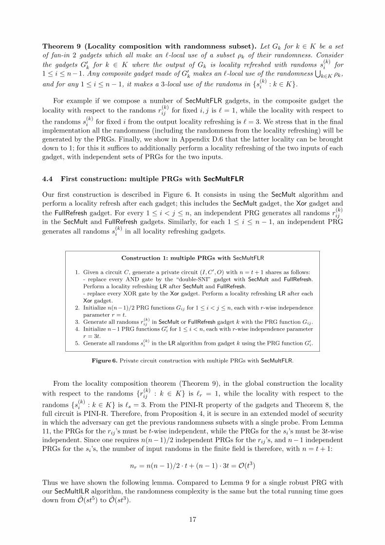
4.4 First construction: multiple PRGs with SecMultFLR

Our first construction is described in Figure 6. It consists in using the SecMult algorithm andperform a locality refresh after each gadget; this includes the SecMult gadget, the Xor gadget and

the FullRefresh gadget. For every 1 ≤ i < j ≤ n, an independent PRG generates all randoms r(k)ij

in the SecMult and FullRefresh gadgets. Similarly, for each 1 ≤ i ≤ n − 1, an independent PRG

generates all randoms s(k)i in all locality refreshing gadgets.

Construction 1: multiple PRGs with SecMultFLR

1. Given a circuit C, generate a private circuit (I, C′, O) with n = t+ 1 shares as follows:- replace every AND gate by the “double-SNI” gadget with SecMult and FullRefresh.Perform a locality refreshing LR after SecMult and FullRefresh.- replace every XOR gate by the Xor gadget. Perform a locality refreshing LR after eachXor gadget.

2. Initialize n(n−1)/2 PRG functions Gij for 1 ≤ i < j ≤ n, each with r-wise independenceparameter r = t.

3. Generate all randoms r(k)ij in SecMult or FullRefresh gadget k with the PRG function Gij .

4. Initialize n−1 PRG functions G′i for 1 ≤ i < n, each with r-wise independence parameterr = 3t.

5. Generate all randoms s(k)i in the LR algorithm from gadget k using the PRG function G′i.

Figure 6. Private circuit construction with multiple PRGs with SecMultFLR.

From the locality composition theorem (Theorem 9), in the global construction the locality

with respect to the randoms {r(k)ij : k ∈ K} is `r = 1, while the locality with respect to the

randoms {s(k)i : k ∈ K} is `s = 3. From the PINI-R property of the gadgets and Theorem 8, the

full circuit is PINI-R. Therefore, from Proposition 4, it is secure in an extended model of securityin which the adversary can get the previous randomness subsets with a single probe. From Lemma11, the PRGs for the rij ’s must be t-wise independent, while the PRGs for the si’s must be 3t-wiseindependent. Since one requires n(n−1)/2 independent PRGs for the rij ’s, and n−1 independentPRGs for the si’s, the number of input randoms in the finite field is therefore, with n = t+ 1:

nr = n(n− 1)/2 · t+ (n− 1) · 3t = O(t3)

Thus we have shown the following lemma. Compared to Lemma 9 for a single robust PRG withour SecMultILR algorithm, the randomness complexity is the same but the total running time goesdown from O(st5) to O(st3).

17

Lemma 12 (multiple PRGs with SecMultFLR). Any function of circuit size s admits a t-private implementation (I, C,O) with the canonic encoder I and decoder O, where C uses O(t3 ·log(st)) bits of randomness, and runs in time O(s · t3 · log2(st)).

4.5 Second construction: multiple PRGs with SecMultILR

Our second construction is described in Figure 7, based on the SecMultILR algorithm. As illustratedin Figure 8, a dedicated PRG generates the rij ’s for a given row i, in all gadgets. We first showthat the SecMultILR algorithm makes a 1-local use of each row of randoms rij and a 2-local use ofeach row of randoms sij ; see Appendix D.7 for the proof.

Lemma 13 (Locality of SecMultILR). The SecMultILR algorithm makes a 1-local use of eachrandomness set ρi = {rij : i < j ≤ n} and a 2-local use of each randomness set ρ′i = {sij : i < j ≤n}.

Construction 2: multiple PRGs with SecMultILR

1. Given a circuit C, generate a private circuit (I, C′, O) with n = t+ 1 shares as follows:- replace every AND gate by the “double-SNI” gadget with SecMultILR and the cor-responding FullRefreshILR. Perform a locality refreshing LR after each SecMultILR andFullRefreshILR.- replace every XOR gate by the Xor gadget. Perform a locality refreshing LR after eachXor gadget.

2. Initialize n−1 PRG functions Gi for 1 ≤ i < n, each with r-wise independence parameterr = t.

3. Generate all randoms r(k)ij in SecMultILR or FullRefreshILR gadget k with the PRG function

Gi.4. Initialize n−1 PRG functions G′i for 1 ≤ i < n, each with r-wise independence parameter

r = 2t.5. Generate all randoms s

(k)ij in SecMultILR or FullRefreshILR gadget k using the PRG func-

tion G′i.6. Initialize n−1 PRG functions G′′i for 1 ≤ i < n, each with r-wise independence parameter

r = 3t.7. Generate all randoms s

(k)i in the LR algorithm using the PRG function G′′i .

Figure 7. Private circuit construction with multiple PRGs with SecMultILR.

From Lemma 13 and Theorem 9, in the global construction the locality with respect to the

subsets of randoms ρi = {r(k)ij : i < j ≤ n, k ∈ K} is equal to 1, the locality with respect to the

subsets of randoms ρ′i = {s(k)ij : i < j ≤ n, k ∈ K} is equal to 2, and the locality with respect to the

subsets of randoms ρ′′i = {s(k)i : k ∈ K} is still equal to 3, for each 1 ≤ i < n. As previously, from

the PINI-R property of the gadgets and Proposition 8, the full circuit is PINI-R. Therefore, it issecure in an extended model of security in which the adversary can get the previous randomnesssubsets with a single probe. From Lemma 11, the corresponding PRGs must therefore have r-wiseindependence parameter r = t, r = 2t and r = 3t respectively. The main difference is that now

there are only n − 1 independent PRGs to generate the r(k)ij (instead of n(n − 1)/2 previously),

because a given PRG generates those randoms for all indices j. The total number of input randomsin the finite field is therefore:

nr = (n− 1) · t+ (n− 1) · 2t+ (n− 1) · 3t = O(t2)

Thus we have shown the following lemma. Asymptotically this is the most efficient technique (seeTable 1 for a comparison), and also the most efficient in practice (see the next section for ourimplementation results on AES).

18

Lemma 14 (multiple PRGs with SecMultILR). Any function of circuit size s admits a t-privateimplementation (I, C,O) with the canonic encoder I and decoder O, where C uses O(t2 · log(st))bits of randomness, and runs in time O(s · t3 · log2(st)).

r(1)ij r

(1)

ij′ r(2)ij r

(2)

ij′ r(s)ij r

(s)

ij′

Gi

ρ′i

Figure 8. In Construction 2, a dedicated PRG generates the rij ’s for a given row i in all gadgets, from a randomseed ρ′i.

5 Application to AES

In this section we describe a concrete implementation of our techniques for AES; the goal is tominimize the total amount of randomness used to protect AES against t-th order attack. Weprovide the source code in C in [Cor13].

5.1 The AES circuit and the Rivain-Prouff countermeasure

To implement the AES SBox, we need to perform 4 multiplications, and 2 mask refreshing perbyte; see [RP10] for the sequence of operations. For the mask refreshing, we use the multiplicationbased refreshing FullRefresh recalled in Appendix B.2. We refer to [BBD+16] for the proof that thex254 gadget is (n− 1)-SNI; this implies that the gadget is PINI. Thus, this amounts to performing6 multiplications per byte. Since there are 16 bytes to process per round, the number of requiredmultiplications is 6 × 16 = 96 per round. Thus for the 10 rounds of the AES, one will perform96× 10 = 960 multiplications.

5.2 Implementation with single robust PRG

We first consider an implementation with a single robust PRG as in Section 3, with 3 possible algo-rithms: the original [IKL+13] construction with a locality refresh after each multiplication gadget(SecMultFLR), and our new SecMultILR and SecMultILR2 algorithms. For those three algorithms,we provide in Table 7 the total number of pseudo-randoms to be generated for the AES circuit, thecorresponding locality parameter `, and the number of 8-bit randoms from the TRNG to generatethe seed of the PRG, as a function of the number of shares n, for security against t probes withn = t+ 1.

We now explain the content of Table 7. For each of the 3 algorithms, the number of pseudo-randoms is the number of randoms from Table 3 in Section 3, multiplied by 960, since one mustperform 960 multiplications. Furthermore, the MixColumns operation requires 48 xors. Normallywe should perform a locality refresh after each xor, but in the particular case of the AES, we cando the locality refresh only after the 3 xors of the MixColumns for each byte. In that case, thelocality parameter with respect to MixColumns is then 4(n − 1), instead of 2(n − 1) for a singlexor. The locality of the global circuit is then the max of locality parameter ` from Table 3 and4(n − 1). Equivalently, we can perform such locality refresh as input of the SubByte operation,

19

SecMult [RP10] SecMultFLR [IKL+13] SecMultILR SecMultILR2

Mult 480n(n− 1) (480n+ 960)(n− 1) 960n(n− 1) (480n+ 960)(n− 1)

Xor − 160(n− 1) 160(n− 1) 160(n− 1)

Pseudo-rand − (480n+ 1120)(n− 1) (960n+ 160)(n− 1) (480n+ 1120)(n− 1)

Locality ` − max(4(n− 1),4(n− 1) 4(n− 1)

n2/4 + 5n/2− c)True-rand 480n(n− 1) 2n(n− 1) ·max(4(n− 1),

8n(n− 1)2 8n(n− 1)2n2/4 + 5n/2− c)

Table 7. For AES, total number of pseudo-randoms and number of 8-bit TRNG calls, for a single robust PRG, asa function of the number of shares n. We have c = 3 for even n, and c = 11/4 for odd n. We assume that n ≤ 12.

which enables to keep the MixColumns unmodified. For the MixColumns, one therefore needs toperform 16 locality refresh per round, which gives a total of 160 locality refresh for the 10 roundsof the AES, which requires 160(n − 1) pseudo-randoms. Finally, we assume that the round keysare already masked without PRG, and so we don’t need to perform a locality refreshing after theAddRoundKey.

Let m the total number of pseudo-randoms over F28 that must be generated. To determine thefinite field F = F28k used by the PRG, we must ensure m ≤ k · |F28k | = k · 28k. Namely a singlepolynomial evaluation over F28k generates k bytes of pseudo-random. One must then use a PRGwith r-wise independence parameter r = ` · (n − 1). Using the trivial construction with the xorof n = t + 1 polynomial evaluations (to provide resistance against t probes), the total number offresh random values over F28 is then nr = k · n · r = k · n(n− 1) · `.

For the three algorithms one can work over F216 for n ≤ 12; therefore for simplicity we takek = 2 in Table 7. For SecMultILR and SecMultILR2, the total number of TRNG calls over F28 isthen nr = k ·n(n−1) ·4(n−1) = 4k ·n(n−1)2 with k = 2 for n ≤ 12, and k = 3 for 13 ≤ n ≤ 229,instead of 480n(n − 1) for the original Rivain-Prouff countermeasure; therefore one needs fewerTRNG calls than Rivain-Prouff for n ≤ 40. We summarize in Table 9 below the number of inputrandom bytes required for AES for small values of n, compared with the original Rivain-Prouffcountermeasure.

5.3 Implementation with multiple PRGs

We now consider an implementation of AES with multiple PRGs, as in Section 4. We consider theSecMultFLR algorithm corresponding to Construction 1, and the SecMultILR algorithm correspond-ing to Construction 2. As previously, we provide in Table 8 the total number of pseudo-randomsto be generated for the AES circuit, and the number of 8-bit randoms from the TRNG.

SecMult [RP10] SecMultFLR SecMultILR

Pseudo-rand − (480n+ 1120)(n− 1) (960n+ 160)(n− 1)

Locality `r of rij − 1 1

Number of PRGs (rij) − n(n− 1)/2 n− 1

True-rand per PRG (rij) − 2(n− 1) 2(n− 1)

Locality `s of sij and si − 5 5

Number of PRGs (si and sij) − n− 1 n− 1

True-rand per PRG (sij and si) − 10(n− 1) 10(n− 1)

Total True-Rand 480n(n− 1) (n+ 10)(n− 1)2 12(n− 1)2

Table 8. For AES, total number of Pseudo-random and True-random values to generate with the multiple PRGsapproach, as a function of the number of shares n. Values for the Rivain-Prouff countermeasure are also recalled forcomparison.

20

As previously, we only perform a locality refresh after the 3 xors of the MixColumns (equiva-lently, before each SubByte). Moreover we don’t perform the LR algorithm after SecMultILR as inConstruction 2, since the output of SecMultILR is already locality refreshed. Therefore the num-ber of pseudo-randoms is the same as in the previous section. We use two classes of independentPRGs. The first class of independent PRGs is used to generate the rij ’s from SecMultFLR andSecMultILR algorithms, with locality `r = 1; therefore the PRGs must be `rt-wise independent. Weneed n(n − 1)/2 such PRGs for SecMultFLR, and only n − 1 for SecMultILR. Working over F216 ,each PRG requires 2`rt = 2(n − 1) random bytes. Similarly, the second class of PRGs is used togenerate randoms si from the locality refresh, and also the randoms sij for the internal localityrefresh in SecMultILR, with locality `s = 5. Namely we only perform the locality refresh after the3 xors of the MixColumns, and therefore the locality is `s = 5 (instead of `s = 3). Note that forSecMultILR we can use the same class of PRGs to generate the randoms sij ’s from SecMultILR andthe randoms si’s from LR, instead of two classes in Construction 2 from Section 4; namely it iseasy to see that the locality with respect to the corresponding randomness subsets is still equalto 5. Therefore the PRGs must be `st-wise independent; working over F216 , each PRG requires10(n− 1) bytes of TRNG.

In summary, for SecMultFLR, the total number of 8-bit TRNG calls is therefore:

nr = n(n− 1)/2 · 2(n− 1) + (n− 1) · 10(n− 1) = (n+ 10)(n− 1)2

and for SecMultILR, we get:

nr = (n− 1) · 2(n− 1) + (n− 1) · 10(n− 1) = 12(n− 1)2

instead of 480n(n− 1) in the original Rivain-Prouff countermeasure.2

A simple 3-wise independent PRG. Finally, we consider the simple 3-wise independent PRGfrom Section 2.3:

G(x1, . . . , xd, y1, . . . , yd) = (xi ⊕ yj)1≤i,j≤d

Since the PRG function G expands from 2d to d2 bits (or bytes), the number of input randomsbecomes O(

√s) instead of O(s), where s is the circuit size. Note that this is worse than the

polynomial-based PRG used previously that requires onlyO(log s) randoms, but the above functionG is very fast since generating a pseudo-random only takes a single xor.

Since the above PRG only achieves 3-wise independence, we want to minimize the locality.Therefore, we perform a locality refresh of the 2 inputs of each gadget (with two distinct sets ofindependent PRGs), and we perform a locality refresh of the outputs of each gadget (SecMult, Xorand FullRefresh), using another distinct set of independent PRGs. As shown in Appendix D.6, thelocality with respect to each subset of randoms is then always ` = 1; therefore, we can use a PRGwith r-wise independence r = t = n− 1. This implies that this specific PRG only works for n = 3and n = 4 shares. We argue in Appendix E.2 that the total number of input bytes for AES is 642for n = 3 and 1056 for n = 4, instead of 2880 and 5760 respectively for the original Rivain-Prouffcountermeasure.

Summary. We summarize in Table 9 the number of input random bytes required for AES forall previous methods, as a function of the number of shares n, in order to achieve t-th ordersecurity, with t = n−1. We see that the most efficient method (in terms of minimizing the numberof TRNG calls) is the SecMultILR algorithm with multiple PRGs. Namely for small values of twe obtain almost two orders of magnitude improvement compared to the original Rivain-Prouffcountermeasure.

2 For the SecMultILR algorithm, a PRG for the sij and si must generate a maximum of 960(n − 1) + 160 pseudo-randoms; therefore one can work over F216 as long as n ≤ 136.

21

Single robust PRG Multiple PRGs

[RP10] [IKL+13] SecMultILR SecMultILR2 SecMultFLR SecMultILR 3-wise SecMultFLR

n = 3 2880 96 96 96 52 48 642

n = 4 5760 288 288 288 126 108 1056

n = 5 9600 640 640 640 240 192 −n = 6 14400 1260 1200 1200 400 300 −n = 7 20160 2268 2016 2016 612 432 −n = 8 26880 3696 3136 3136 882 588 −n = 9 34560 5760 4608 4608 1216 768 −n = 10 43200 8460 6480 6480 1620 972 −

Table 9. For AES, total number of TRNG bytes to generate for single and multiple PRGs methods, depending ofthe number of shares n. We also provide the number of TRNG bytes for the original Rivain-Prouff countermeasure.

5.4 Concrete Implementation

We have implemented our constructions for AES in C, on a 44 MHz ARM-Cortex M3 processor.The processor is used in a wide variety of products such as passports, bank cards, SIM cards, secureelements, etc. The embedded TRNG module can run in parallel of the CPU, but it is relativelyslow: according to our measurements on emulator, it outputs 32 bits of random in approximately6000 cycles. Our results, obtained by running the code on emulator, are given in Table 10, and arecompared with the classical Rivain-Prouff countermeasure.

We see that in practice the most efficient countermeasure is the SecMultFLR algorithm withmultiple PRGs, using the 3-wise independent PRG. For n = 3 and n = 4 we obtain a 52% and61% speedup respectively, compared to Rivain-Prouff. We provide the source code in [Cor13].

Single robust PRG Multiple PRGs

[RP10] SecMultFLR SecMultILR SecMultILR2 SecMultFLR SecMultILR 3-wise SecMultFLR

n = 3Mcycles 20.6 65.6 76.8 65.4 12 14.1 9.8

ratio 1 3.18 3.73 3.17 0.58 0.68 0.48

n = 4Mcycles 40.2 235.1 425.1 324.9 24.6 34.7 15.5

ratio 1 5.85 10.57 8.08 0.61 0.86 0.39

n = 5Mcycles 65.8 1100 1541.5 1097.1 42.8 70 −

ratio 1 16.72 23.43 16.67 0.65 1.06 −

n = 6Mcycles 97.5 3042.1 4278.3 2898.5 67.2 124.1 −

ratio 1 31.20 43.88 29.73 0.69 1.27 −

Table 10. Smart-card implementation results, on a 44 MHz ARM-Cortex M3 processor, with an embedded TRNGmodule. We provide the timings in millions of clock cycles, and the ratio with respect to the Rivain-Prouff counter-measure.

References

[AIS18] Prabhanjan Ananth, Yuval Ishai, and Amit Sahai. Private circuits: A modular approach. In Advancesin Cryptology - CRYPTO 2018 - Proceedings, Part III, pages 427–455, 2018. Final version available athttps://eprint.iacr.org/2018/566.pdf.

[BBD+15] Gilles Barthe, Sonia Belaıd, Francois Dupressoir, Pierre-Alain Fouque, Benjamin Gregoire, and Pierre-Yves Strub. Verified proofs of higher-order masking. In Advances in Cryptology - EUROCRYPT 2015 -Proceedings, Part I, pages 457–485, 2015.

[BBD+16] Gilles Barthe, Sonia Belaıd, Francois Dupressoir, Pierre-Alain Fouque, Benjamin Gregoire, Pierre-YvesStrub, and Rebecca Zucchini. Strong non-interference and type-directed higher-order masking. In Pro-ceedings of the 2016 ACM SIGSAC Conference on Computer and Communications Security, Vienna,Austria, October 24-28, 2016, pages 116–129, 2016. Publicly available at https://eprint.iacr.org/

2015/506.pdf.

22

[BBP+16] Sonia Belaıd, Fabrice Benhamouda, Alain Passelegue, Emmanuel Prouff, Adrian Thillard, and DamienVergnaud. Randomness complexity of private circuits for multiplication. In Advances in Cryptology -EUROCRYPT 2016 - Proceedings, Part II, pages 616–648, 2016.

[Cor13] Jean-Sebastien Coron. Implementation of higher-order countermeasures, 2013. Publicly available athttps://github.com/coron/htable/.

[Cor17] Jean-Sebastien Coron. CheckMasks: formal verification of side-channel countermeasures, 2017. Publiclyavailable at https://github.com/coron/checkmasks.

[Cor18] Jean-Sebastien Coron. Formal verification of side-channel countermeasures via elementary circuit trans-formations. In Applied Cryptography and Network Security ACNS, volume 10892, pages 65–82, 2018.

[CS18] Gaetan Cassiers and Francois-Xavier Standaert. Trivially and efficiently composing masked gadgets withprobe isolating non-interference. Cryptology ePrint Archive, Report 2018/438, 2018. https://eprint.

iacr.org/2018/438.[DDF14] Alexandre Duc, Stefan Dziembowski, and Sebastian Faust. Unifying leakage models: From probing attacks

to noisy leakage. In Advances in Cryptology - EUROCRYPT 2014 - Proceedings, pages 423–440, 2014.[FPS17] Sebastian Faust, Clara Paglialonga, and Tobias Schneider. Amortizing randomness complexity in private

circuits. In Advances in Cryptology - ASIACRYPT 2017 - Proceedings, Part I, pages 781–810, 2017.[GUV09] Venkatesan Guruswami, Christopher Umans, and Salil P. Vadhan. Unbalanced expanders and randomness

extractors from parvaresh-vardy codes. J. ACM, 56(4):20:1–20:34, 2009.[IKL+13] Yuval Ishai, Eyal Kushilevitz, Xin Li, Rafail Ostrovsky, Manoj Prabhakaran, Amit Sahai, and David

Zuckerman. Robust pseudorandom generators. In ICALP 2013, Proceedings, Part I, pages 576–588,2013.

[ISW03] Yuval Ishai, Amit Sahai, and David Wagner. Private circuits: Securing hardware against probing attacks.In Advances in Cryptology - CRYPTO 2003, Proceedings, pages 463–481, 2003.

[OMHT06] Elisabeth Oswald, Stefan Mangard, Christoph Herbst, and Stefan Tillich. Practical second-order DPAattacks for masked smart card implementations of block ciphers. In CT-RSA, pages 192–207, 2006.

[RP10] Matthieu Rivain and Emmanuel Prouff. Provably secure higher-order masking of AES. In CryptographicHardware and Embedded Systems, CHES 2010, Proceedings, pages 413–427, 2010.

A PRG based on bipartite expander graph

A.1 Definitions

Bipartite graph and PRG. We note by [n] the set of integers between 1 and n. A bipartite graphis a triple ([m], [n], E) where [m] is the set of left vertices, [n] of right vertices, and E ⊂ [m]×[n] is aset of edges connecting the left vertices with the right vertices. Given any subset V ⊆ [m], we denoteby Γ (V ) the right neighbors of V ; formally Γ (V ) = {v ∈ [n] : ∃u ∈ [m] such that (u, v) ∈ E}.

1

2

3

4

5

6

7

8

9

y1 = x1 ⊕ x4y2 = x2 ⊕ x4y3 = x3 ⊕ x4

y4 = x1 ⊕ x5y5 = x2 ⊕ x5y6 = x3 ⊕ x5

y7 = x1 ⊕ x6y8 = x2 ⊕ x6y9 = x3 ⊕ x6

3

2

1

4

5

6

x1

x2

x3

x4

x5

x6

Figure 9. Example of a ([m], [n], E) bipartite graph with m = 9 and n = 6, with the corresponding PRG. The graphis a (2, 3/2)-expander.

We recall the simple construction of a PRG from bipartite graph [IKL+13]. A bipartite graphH = ([m], [n], E) induces a linear function GH : {0, 1}n → {0, 1}m where the i-th output bitfor 1 ≤ i ≤ m is the parity of the input bits corresponding to the neighbors of i. Formally,

23

GH(x1, . . . , xn) = (y1, . . . , ym) where yi = ⊕j∈Γ (i)xj . In other words, every left vertex gives anoutput bit, computed as the xor of the input bits corresponding to the right vertices to which it isconnected. See Figure 9 for an example of a simple bipartite graph, with the corresponding PRG.

Expander graphs. Letting V ⊂ [m] on the left, a vertex v ∈ [n] on the right is said to be aunique neighbor of V if there is a single edge from V to v. We let U(V ) denote the collection ofunique neighbors of V . We say that a bipartite graph ([m], [n], E) is a `-unique neighbor expanderif any set V ⊂ [m] on the left with |V | ≤ ` has a unique neighbor.

Lemma 15. If a bipartite graph H = ([m], [n], E) is a `-unique neighbor expander, then the cor-responding PRG GH is `-wise independent.

Proof. We consider the m×n matrix of row vectors corresponding to the linear function GH(x1, . . ., xn). We show that any subset of at most ` rows are linearly independent. Namely a linear combi-nation of at most ` rows cannot be equal to 0, since by the `-unique neighbor expander property,there is an input xi that must appear in a single row. Since any subset of at most ` rows arelinearly independent, the PRG GH is `-wise independent. ut

Expander graphs. To construct bipartite graphs with the unique neighbor property, we will useexpander graphs.

Definition 11. A bipartite graph ([m], [n], E) with left vertices [m] and right vertices [n] is an(`, b)-expander if for any subset V ⊆ [m] on the left with |V | ≤ `, we have that |Γ (V )| ≥ b|V |.

The following lemma shows that if the expansion factor b is such that b > d/2, then any set V suchthat |V | ≤ ` has a unique neighbor; therefore the corresponding PRG will be `-wise independent.

Lemma 16. Consider an (`, b)-expander graph ([m], [n], E) of degree d. For any V ⊂ [m] with|V | ≤ `,

d|V | ≥ |Γ (V )| ≥ |U(V )| ≥ (2b− d)|V |

Proof. The number of edges out of V is d|V |, so d|V | ≥ |Γ (V )|. Out of these d|V | edges, due to theexpansion property of the graph, at least b|V | go to distinct vertices; there remains (d−b)|V | edges,which can eliminate the uniqueness of at most (d − b)|V | vertices in Γ (V ). Therefore |U(V )| ≥b|V | − (d− b)|V | ≥ (2b− d)|V |. ut

A.2 A simplified proof of strong robustness for PRG

In this section we provide a simplified proof of strong robustness of PRG based on expander graph.

Theorem 10 ([IKL+13]). Suppose H is a d-left-regular (`, d/2 + c)-expander. Then GH is astrong (`, c`/d, d/c)-robust PRG.

The proof of Theorem 10 is based on the lemma below, showing that an expander graph isrobust against the removal of vertices; that is, even if we remove some vertices on the right,the induced graph remains an expander graph. More precisely, the following lemma is a slightlystronger variant of [IKL+13, Lemma 6], which was used to prove the PRG weak robustness only.The difference is that in our lemma the induced graph has right vertices [n] \ (S ∪ Γ(T )) insteadof only [n] \ S; that is, we remove more vertices on the right. Another difference is that for theresulting graph we only get the `-unique neighbor property (instead of the expansion property),since this is only what we need. The rest of the proof is essentially the same as in [IKL+13].

Lemma 17. Suppose H = ([m], [n], E) is a d-left-regular (`, d/2 + c)-expander. Then for anyS ⊆ [n] on the right of size |S| ≤ c`, there exists T ⊆ [m] on the left with |T | ≤ |S|/c such thatthe induced graph on left vertices [m] \ T and right vertices [n] \ (S ∪ Γ(T )) is a (` − |T |)-uniqueneighbor expander.

24

Proof. We first construct a subset T on the left with a large fraction of its right neighbors Γ(T )in S. We let T be a subset on the left that has the maximum size among all subsets T ′ on the leftwith size at most ` such that |Γ(T ′) \ S| ≤ d/2 · |T ′|; the set T is well defined because T ′ = ∅ issuch a subset. We have by definition of T :

|Γ(T )| = |Γ(T ) \ S|+ |Γ(T ) ∩ S| ≤ d/2 · |T |+ |Γ(T ) ∩ S|

From the expansion property of H and |T | ≤ `, we must have:

|Γ(T )| ≥ (d/2 + c)|T |

Combining the two inequalities, we get:

|Γ(T) ∩ S| ≥ |Γ(T )| − d/2 · |T | ≥ c · |T |

which shows that T has a large fraction of neighbors in S. We obtain |T | ≤ |Γ(T) ∩ S|/c ≤ |S|/cas required.

We now consider any non-empty subset V on the left with V ∩T = ∅ and |V | ≤ `−|T |. We showthat V must have many neighbors outside the set S ∪Γ(T ). Namely T ∪V has many neighbors bythe expansion property, and the neighbors of T are fairly concentrated in S. More precisely, since|T ∪ V | = |T | + |V | ≤ ` and T was selected as a subset of maximal size with size at most ` suchthat |Γ(T ) \ S| ≤ d/2 · |T |, we must have:

|Γ(T ∪ V ) \ S| > d/2 · |T ∪ V | = d/2 · (|T |+ |V |)

Moreover we have:

|Γ(T ∪ V ) \ S| =∣∣(Γ(T ) ∪ Γ(V )) \ S

∣∣ = |Γ(T ) \ S|+∣∣Γ(V ) \ (Γ(T ) ∪ S)

∣∣Using |Γ(T ) \ S| ≤ d/2 · |T |, we obtain:∣∣Γ(V ) \ (Γ(T ) ∪ S)

∣∣ = |Γ(T ∪ V ) \ S| − |Γ(T ) \ S|> d/2 · (|T |+ |V |)− d/2 · |T |> d/2 · |V |

This shows that the induced graph on left vertices [m] \ T and right vertices [n] \ (S ∪ Γ(T )) is a(`− |T |)-unique neighbor expander. ut

Proof (of theorem 10). Let t ≤ k be the number of probes in the circuit, with k = c`/d. Let S bethe vertices on the right that are affected by the probes. Since every output is the sum of exactlyd randoms, we must have |S| ≤ td ≤ kd = c`. Therefore we can apply Lemma 17, and there existsa set T on the left with |T | ≤ |S|/c ≤ td/c such that the induced graph on left vertices [m] \ Tand right vertices [n] \ (S ∪ Γ(T )) is a (`− |T |)-unique neighbor expander. We let S′ = S ∪ Γ(T ).Therefore, conditioned on any fixing of the input bits in S′, the input bits in S are fixed and theoutput bits in T are fixed (because the input bits in Γ (T ) are fixed), and the output bits that arenot in T are r-wise independent, where r = `− |T | ≥ `− td/c, which gives q = d/c. ut

A.3 The bipartite expander graph construction from [GUV09]

In this section we recall the bipartite expander graph construction from [GUV09], and its appli-cation to PRG. We fix the field Fq. Let E(Y ) be an irreducible polynomial of degree n over Fq.We identity elements of Fnq with univariate polynomials over Fq with degree at most n− 1. Let hbe an integer parameter. Let d ≤ q. The expander is the bipartite graph Γ : Fnq × [d] → [d] × Fmqdefined as:

Γ(f, i)def= [i, f(i), (fh mod E)(i), (fh

2mod E)(i), . . . , (fh

m−1mod E)(i)]

Theorem 11 ([GUV09]). The graph Γ : Fnq × [d]→ [d]×Fq defined above is a (hm, A) expanderfor A = d− (n− 1)(h− 1)m.

The above graph expander is therefore defined by the following 5 parameters: q, n, d, m andh. Therefore, finding the right parameters is not obvious. In the following we study two possibleregimes.

25

Minimizing the input randomness. In this regime, we want to minimize the size of the inputrandomness of the r-wise independent PRG. We fix the parameter m. Therefore we must havehm ≥ r, so we take h = dr1/me. The PRG takes as input dqm ≤ qm+1 random bits and outputsqn pseudo-randoms, so we take n = m + 1, so that the PRG is at least expanding. For minimalrobustness, we take A > d/2, which gives the condition q > d > 2(n − 1)(h − 1)m. Thereforewe take d = q − 1 and q the smallest prime greater than 2(n − 1)(h − 1)m + 2. Recall that thetrivial construction based on polynomial evaluation can achieve r-wise independence and resistanceagainst r probes with r(r+ 1) input randoms. To do better than the trivial construction, one musttherefore ensure that dqm < r(r + 1). As illustrated in Table 11, the PRG based on expandergraph becomes better than the trivial construction only for r ≥ 218, which requires at least 236

input random bits. Therefore, if the goal is to use fewer TRNGs than the trivial construction, theconstruction of expander graphs based on [GUV09] is totally impractical.

r-wise independence 218 222 230 240

m 2 2 2 2

h 512 2048 32768 220

q 4091 16381 262139 ' 223

Number of input bits dqm 236 242 254 269

Table 11. Parameters of the PRG based on the [GUV09] bipartite expander graph.

Small d regime. In this regime, we want to minimize the degree d for a given r, in orderto minimize the time of pseudo-random generation. For simplicity we only require the r-wiseindependence. Therefore we can take d = 2(n− 1)m(h− 1) + 1 and we must have hm ≥ r; we taken = m+ 1. We provide the result in Table 12. For large values of m, we can use the approximationh = r1/m and d = 2m2h. We must therefore minimize the function f(m) = 2m2r1/m, and we findthat the function is minimized for m = log r, which gives d = O(log2 r). Therefore expander graphscan be used to minimize the time generation of pseudo-randoms.

d 2 3 · · · 54 55 65 73 89 91 97 109 127 129 145 151 161 181 193

r 2 3 · · · 54 64 81 125 144 216 256 343 512 625 729 1024 1296 1331 2401

Table 12. Maximal value of r-wise independence parameter r achievable for a given degree d.

B Definitions and Previous Work

B.1 Security Definition

The PINI security notion. We actually use a slightly simplified definition compared to [CS18],in which the authors define t-PINI where t1 + t2 ≤ t, where t1 is the number of intermediatevariables and |O| = t2, and we must have |I| ≤ t1. In our definition we do not set an upper boundon the total number of variables t that must be simulated, as this appears to be unnecessary. Clearlya gadget that is PINI under our definition is t-PINI under [CS18] for any t ∈ N. Conversely, agadget that is (n−1)-PINI under [CS18] is actually t-PINI for any t ∈ N, and therefore PINI underour definition. Namely it must be t-PINI for any t < n; and for t ≥ n, if t1 + t2 ≥ n, we can takeI = [1, n] \ O, and all intermediate variables can be perfectly simulated knowing all input sharesfrom I ∪ O = [1, n], with |I| = n− |O| = n− t2 ≤ t1; therefore it is t-PINI also for any t ≥ n.

26

Proof of Proposition 2 (PINI composition [CS18]). As in [CS18], we consider l GadgetsG1, · · · , Gl that we order as a direct acyclic graph from output to input in a reverse topologicalsort order. We assume that each gadget Gi has ti internal probes and that the sum of all internalprobes is equal to t. Furthermore, the last gadget G1 has O output probes. We prove by recurrenceon i that the composition of PINI gadgets remains PINI.

If i = 1, then there is only one gadget and this is straightforward since by assumption the gadgetis PINI. Now we assume that the composition of gadgets G1, · · · , Gi is PINI and we prove that thecomposition of gadgets G1, · · · , Gi+1 is still PINI. Since the composition of gadgets G1, · · · , Gi isPINI, we get that for any set of t1 + · · · + ti intermediate variables and any subset O of outputindices, there exists a subset Ii ⊂ [1, n] of input indices with |Ii| ≤ t1 + · · · + ti such that thet1 + · · ·+ ti intermediate variables and the output shares yO,? can be perfectly simulated from theinput shares xIi∪O,?. Furthermore, since gadget Gi+1 is PINI, one can simulate Gadget Gi+1 withinput shares corresponding to indices in Si+1 ∪ (Ii ∪ O) with |Si+1| ≤ ti+1.

Therefore we can compose these simulators to perfectly simulate the composition of gadgetsG1, · · · , Gi+1 from Ii+1 ∪ O with Ii+1 = Si+1 ∪ Ii, and since

|Ii+1| = |Si+1 ∪ Ii| ≤ |Si+1|+ |Ii| ≤ ti+1 + (t1 + · · ·+ ti) ≤ t

we conclude that the composition of i+ 1 gadgets PINI remains PINI.For i+1 = l, we get that we can perfectly simulate the composition of gadgets G1, · · · , Gl from

Il ∪ O with |Il| = |⋃i=li=1 Si| ≤ t1 + · · ·+ tl ≤ t. This terminates the proof.

B.2 Basic gadgets SecMult and FullRefresh

We recall in Algorithm 4 the SecMult gadget used in [RP10] for protecting AES against t-th orderattacks. It is an extension to F2k of the original ISW countermeasure [ISW03] described in F2. TheSecMult gadget was proven t-SNI in [BBD+16].

Algorithm 4 SecMultInput: shares ai satisfying

⊕ni=1 ai = a, shares bi satisfying

⊕ni=1 bi = b

Output: shares ci satisfying⊕n

i=1 ci = a · b1: for i = 1 to n do2: ci ← ai · bi3: end for4: for i = 1 to n do5: for j = i+ 1 to n do6: r ← F2k # referred by ri,j7: ci ← ci ⊕ r # referred by ci,j8: r ← (ai · bj ⊕ r)⊕ aj · bi # referred by rj,i9: cj ← cj ⊕ r # referred by cj,i

10: end for11: end for12: return (c1, . . . , cn)

The mask refreshing gadget FullRefresh recalled in Algorithm 5 was introduced by Duc et. alin [DDF14]; it was proven t-SNI in [BBD+16].

B.3 Proof of Lemma 1 (3-wise independence of G)

One must show that any set of three values among all (xi ⊕ yj)1≤i,j≤d values, remains uniformlyand independently distributed.

Thus, we consider three outputs of the PRGs, namely (xi1 ⊕ yj1), (xi2 ⊕ yj2) and (xi3 ⊕ yj3).Three cases arise: if we have i1 6= i2 6= i3, then the three values are independent thanks to randomsxi1 , xi2 and xi3 . If we have i1 = i2 = i3, then we must have j1 6= j2 6= j3 and the three values are

27

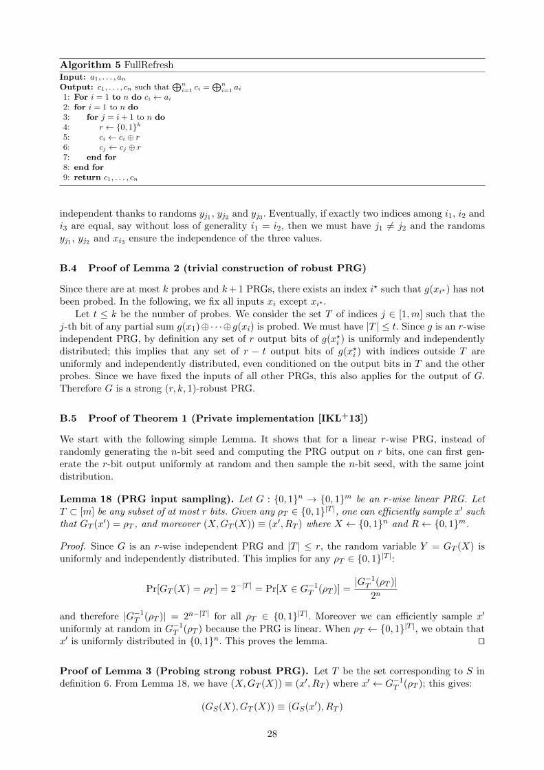
Algorithm 5 FullRefreshInput: a1, . . . , anOutput: c1, . . . , cn such that

⊕ni=1 ci =

⊕ni=1 ai

1: For i = 1 to n do ci ← ai2: for i = 1 to n do3: for j = i+ 1 to n do4: r ← {0, 1}k5: ci ← ci ⊕ r6: cj ← cj ⊕ r7: end for8: end for9: return c1, . . . , cn

independent thanks to randoms yj1 , yj2 and yj3 . Eventually, if exactly two indices among i1, i2 andi3 are equal, say without loss of generality i1 = i2, then we must have j1 6= j2 and the randomsyj1 , yj2 and xi3 ensure the independence of the three values.

B.4 Proof of Lemma 2 (trivial construction of robust PRG)

Since there are at most k probes and k+ 1 PRGs, there exists an index i? such that g(xi?) has notbeen probed. In the following, we fix all inputs xi except xi? .

Let t ≤ k be the number of probes. We consider the set T of indices j ∈ [1,m] such that thej-th bit of any partial sum g(x1)⊕· · ·⊕g(xi) is probed. We must have |T | ≤ t. Since g is an r-wiseindependent PRG, by definition any set of r output bits of g(x?i ) is uniformly and independentlydistributed; this implies that any set of r − t output bits of g(x?i ) with indices outside T areuniformly and independently distributed, even conditioned on the output bits in T and the otherprobes. Since we have fixed the inputs of all other PRGs, this also applies for the output of G.Therefore G is a strong (r, k, 1)-robust PRG.

B.5 Proof of Theorem 1 (Private implementation [IKL+13])

We start with the following simple Lemma. It shows that for a linear r-wise PRG, instead ofrandomly generating the n-bit seed and computing the PRG output on r bits, one can first gen-erate the r-bit output uniformly at random and then sample the n-bit seed, with the same jointdistribution.

Lemma 18 (PRG input sampling). Let G : {0, 1}n → {0, 1}m be an r-wise linear PRG. LetT ⊂ [m] be any subset of at most r bits. Given any ρT ∈ {0, 1}|T |, one can efficiently sample x′ suchthat GT (x′) = ρT , and moreover (X,GT (X)) ≡ (x′, RT ) where X ← {0, 1}n and R← {0, 1}m.

Proof. Since G is an r-wise independent PRG and |T | ≤ r, the random variable Y = GT (X) isuniformly and independently distributed. This implies for any ρT ∈ {0, 1}|T |:

Pr[GT (X) = ρT ] = 2−|T | = Pr[X ∈ G−1T (ρT )] =

|G−1T (ρT )|

2n

and therefore |G−1T (ρT )| = 2n−|T | for all ρT ∈ {0, 1}|T |. Moreover we can efficiently sample x′

uniformly at random in G−1T (ρT ) because the PRG is linear. When ρT ← {0, 1}|T |, we obtain that

x′ is uniformly distributed in {0, 1}n. This proves the lemma. ut

Proof of Lemma 3 (Probing strong robust PRG). Let T be the set corresponding to S indefinition 6. From Lemma 18, we have (X,GT (X)) ≡ (x′, RT ) where x′ ← G−1

T (ρT ); this gives:

(GS(X), GT (X)) ≡ (GS(x′), RT )

28

From |L \ T | ≤ |L| ≤ r − q|S| and the strong (r, q, k)-robustness of G, we have that GL\T (X) isuniform and independent from (GS(X), GT (X)). Therefore:

[(GL\T (X), GT (X)) |GS(X) = gS , GT (X) = gT ] ≡ [RL∪T |RT = gT ]

Since the distribution of x′ only depends on gT , we have:

[RL∪T |RT = gT ] ≡ [RL∪T |GS(x′) = gS , RT = gT ]

Combining the two equations, we get:

[GL∪T (X) |GS(X) = gS , GT (X) = gT ] ≡ [RL∪T |GS(x′) = gS , RT = gT ]

Combining with the first equation, we get

(GL∪T (X), GS(X), GT (X)) ≡ (RL∪T , GS(x′), RT )

and therefore:(GL∪T (X), GS(X)) ≡ (RL∪T , GS(x′))

Therefore the distribution of Y = GL∪T (X) is uniform in {0, 1}|L∪T | when X ← {0, 1}n andmoreover GS(X) can be efficiently simulated given YT only.

Proof of Theorem 1. Consider the k probes in the circuit C ′ distributed as follows: let t be thenumber of probes in the PRG and k−t be the number of probes in the circuit C. Since C makes an`-local use of its randomness, the probes in C can depend on at most (k− t) · ` bits of randomness.From Lemma 3, the output of r− qt bits of the PRG can be replaced by a TRNG, while at mostqt bits of output are required for the simulation of the t probes of the PRG. Therefore, we mustensure:

(k − t) · ` ≤ r − qt

If q ≤ `, then from r ≥ k` we get (k− t) · ` = k`− `t ≤ r− qt as required. If q ≥ ` then from r ≥ kqwe get (k− t) · ` ≤ (k− t) · q = kq− qt ≤ r− qt as required. Eventually, the k probes in C ′ can beperfectly simulated by using

q · t+ (k − t) ≤ q · t+ q(k − t) ≤ qk

probes in the original qk-private circuit C. Therefore, the circuit C ′ is a k-private implementationof f .

B.6 Proof of Lemma 4 (PINI security of LR)

We consider the following simple gadget G: (x1, xn)→ (s1, xn ⊕ (x1 ⊕ s1)), where s1 is a randomvalue. We start by showing that in Gadget G, we can always simulate t probes and |O| outputvariables from the input shares x|I∪O , with |I| ≤ t.

If t + |O| ≥ 2, we can let I = {1, n} \ O which gives I ∪ O = {1, n} and all variables canbe simulated from the input shares x|I∪O . Moreover we have |I| = |{1, n} \ O| ≤ 2 − |O| ≤ t. Ift + |O| = 1, we distinguish two cases. If |O| = 1 and t = 0, then we can simulate either s1 orxn ⊕ (x1 ⊕ s1) by generating a random value. If t = 1 and |O| = 0, we can simulate x1 or xn withI = {1} or I = {n}; the other variables can be simulated by a random value.

We now consider the following gadget Gi for 1 ≤ i ≤ n− 1:

Gi : (x1, . . . , xi, . . . , xn)→ (x1, . . . , xi−1, si, xi+1, . . . , xn ⊕ (xi ⊕ si))

which is similar to Gadget G, but with n input shares instead of 2, and n − 2 unmodified inputshares. As previously, we can always simulate t probes and |O| output variables from the inputshares x|I∪O , with |I| ≤ t. This implies that the gadget Gi is PINI. Since the LR gadget is thecomposition of G1, . . . , Gn−1, from Proposition 2 the LR gadget is also PINI.

29

B.7 Proof of Lemma 5 (Private circuit with PRG)

We first compute the concrete locality ` of the SecMultFLR algorithm. We assume that n ≥ 3. TheSecMult gadget takes as input two sets of shares ai and bi for 1 ≤ i ≤ n and we assume that thoseshares correspond to previous outputs of a locality refresh LR. Therefore those shares are suchthat for 1 ≤ i ≤ n − 1, the shares ai and bi are random values and the shares an and bn dependrespectively on the n − 1 random values ai and bi. As a consequence, the variable anbn which iscomputed within the SecMult Gadget depends on `I = 2(n − 1) random values, i.e. on all inputrandoms.

Furthermore in the SecMult Gadget, n(n − 1)/2 fresh randoms are generated. The variableswhich have the largest dependence to the fresh randoms are the output shares ci; one can see thateach output ci depends on exactly n−1 fresh randoms. In particular, the output cn which includesthe value anbn depends on n− 1 fresh randoms and on the `I input randoms.

Now we investigate the locality refreshing LR performed after SecMult. Within LR, all outputsyi are fresh randoms i.e. they depend on one random value si, except for the last output yn which

depends on those fresh randoms si and on all inputs ci. More precisely, we have: y(0)n = cn and

y(i)n = y

(i−1)n ⊕ (ci ⊕ si), where the last output is yn = y

(n−1)n . Therefore we must investigate all

intermediate values y(i)n for 0 ≤ i ≤ n − 1 to determine which one depends on the most random

values. Note that since all values y(i)n include the share cn, they all depend on at least `I + (n− 1)

random values.By construction of the ci output shares in the SecMult Gadget, each ci depends on exactly n−1

fresh random values. Furthermore, if we take an arbitrary share ci with i < n, we know that ci andcn have exactly one random value in common. Therefore knowing that the shares cn and ci dependrespectively on n−1 random values, the value cn⊕ ci will depend on (n−1) + (n−1)−2 = 2n−4random values since the ⊕ operation removes the common random in both cn and ci. Thus, for

example, the value y(1)n = cn ⊕ (c1 ⊕ s1) depends on `I + 2n − 4 + 1 random values since a new

random s1 is included. With `I = 2(n− 1), we get that y(1)n depends on 4n− 5 random values.

More generally, if we consider the xor of i+1 output shares ck, we know that they have exactly∑ij=1 j random values in common among the fresh random values. Therefore, if we omit for now

the dependence to input randoms `I , the variable cn ⊕ c1 ⊕ · · · ⊕ ci depends on

`C = (i+ 1)(n− 1)− 2

i∑j=1

j =

i∑j=0

(n− 1− 2j)

random values. The value `C increases with the number of shares i provided that 2i ≤ n− 1 andis maximized for i = b(n− 1)/2c, where we have:

`C =

b(n−1)/2c∑j=0

(n− 1− 2j) =

⌊n2

4

⌋.

Therefore the maximum dependence with random values is reached with the variable cn⊕ c1⊕· · · ⊕ cb(n−1)/2c. Therefore in the locality refreshing LR, we deduce that the intermediate variablewhich has the largest dependency to random values is

y(b(n−1)/2c)n = cn ⊕ (s1 ⊕ c1)⊕ · · · ⊕ (s(b(n−1)/2c) ⊕ c(b(n−1)/2c)) .

As a consequence, this value has additional dependence to `R random values si where `R =⌊n−1

2

⌋.

In conclusion, the locality parameter ` is as follows:

` = `I + `C + `R = 2(n− 1) +

⌊n2

4

⌋+

⌊n− 1

2

⌋.

The SecMult algorithm followed by a final locality refresh (SecMultFLR) is therefore an `-localgadget with ` = n2/4 + 5n/2− c, where c = 3 for even n, and c = 11/4 for odd n. With n = t+ 1we have ` = O(t2)

30

The trivial construction of xoring (t+ 1) r-wise independent PRGs based on polynomial evalu-ation, use (t+ 1) · r · log2 |F| bits of randomness and can generate m bits of output, where m ≤ |F|.From Theorem 1 we must set r = t · `; with ` = O(t2), we get r = O(t3). Let s be the originalunprotected circuit size. We need m = O(s · t2) bits of randomness with the ISW construction,therefore we can have log2 |F| = O(log s+ log t), and therefore the total amount of input random-ness with the robust PRG is O(t4 · (log s + log t)) = O(t4). Each pseudo-random generation alsotakes O(t4) time; therefore the circuit runs in time O(s · t6) with the trivial construction.

B.8 Proof of Theorem 2 (Composition of `-local gadgets)

As in the proof of PINI composition in [CS18], we consider m gadgets G1, · · · , Gm that we orderas a direct acyclic graph from output to input in a reverse topological sort order. We assume thateach gadget Gi makes an `-local use of its randomness, with locality refreshed outputs. We proveby recurrence on n that the composition of `-local gadgets is `-local.

If n = 1, then there is only one gadget and this is straightforward since by assumption thegadget is `-local. Now we assume that the composition of gadgets G1, · · · , Gn is `-local and weprove that the composition of gadgets G1, · · · , Gn+1 is still `-local. Since the composition of gadgetsG1, · · · , Gn is `-local, and since by definition the inputs of the gadget Gn are locality refreshedbecause they correspond to outputs of Gadget Gn+1 which are locality refreshed, we get that thecomposition of both parts Gn+1 and G1, · · · , Gn does not increase the global locality. Namely, theglobal locality corresponds to the maximum locality between both parts. Since the composition ofgadgets G1, · · · , Gn is `-local and since Gadget Gn+1 is also `-local, the maximum locality is ` andthe composition of gadgets G1, · · · , Gn+1 is `-local.

C Improving the locality of the multiplication gadget

C.1 Proof of Lemma 8 (locality of SecMultILR)

We consider the SecMultILR algorithm which takes as input two sets of shares ai and bi for 1 ≤ i ≤ nand we assume that those shares are already locality refreshed. Therefore the shares ai and bi arerandom values for 1 ≤ i ≤ n−1 and the shares an and bn depend respectively on the n−1 randomvalues ai and bi. As a consequence, the variable anbn which is computed within the gadget dependson 2(n− 1) random values.

The SecMultILR algorithm consists of a main loop divided into two sub-loops: a first sub-loopA performing the ISW multiplication (lines 5 to 10), and a second loop B performing the localityrefreshing (lines 11 to 15).

In the following, we assume that n ≥ 3 and we prove by recurrence for 2 ≤ j ≤ n− 1 that thevariable cj,j−2 (or c2,1 if j = 2) in loop B has a dependence to 4j − 3 random values, which is themaximal dependence to random values at loop j.

Base case: for j = 2, in Loop A, the variable c2,1 = a2b2 ⊕ (a1b2 ⊕ r1,2 ⊕ a2b1) depends on the4 input random values a1, a2, b1, b2 and on the fresh random r1,2 with a total of 5 random values.Furthermore in Loop B, the variable c2,1 = (a2b2 ⊕ a1b2 ⊕ r1,2 ⊕ a2b1)⊕ ((a1b1 ⊕ r1,2)⊕ s1,2) stilldepends on the 4 input random values a1, a2, b1, b2, and on the fresh random value s1,2, but it doesnot depend anymore on r1,2 which disappears with the ⊕ operation. Therefore, the variable c2,1 inloop A and B has a dependence to 5 = 4j − 3 random values with j = 2.

Recurrence step: now, we assume that for j = k, the value ck,k−2 in Loop A and B has amaximal dependence to 4k − 3 random values and we show that for j = k + 1, the value ck+1,k−1

in Loop B has a dependence to 4(k + 1) − 3 = 4k + 1 random values. We start by analyzingLoop A at round j = k + 1, and more precisely we consider the values ck,k+1 and ck+1,k i.e.values at lines 7 and 9 at loop i = j − 1 = k. The value ck+1,k depends on all inputs ai and bifor 1 ≤ i ≤ k + 1 and on k fresh random values r1,k+1, . . . , rk,k+1, which gives a dependence to2(k + 1) + k = 3k + 2 random values, which is smaller than 4k + 1. Furthermore, the value ck,k+1

is such that ck,k+1 = ck,k−1 ⊕ rk,k+1 and since by recurrence hypothesis the value ck,k−1 has a

31

dependence to at most 4k − 3 random values, the value ck,k+1 depends on (4k − 3) + 1 = 4k − 2random values, which is still smaller than 4k + 1. Therefore in Loop A, we have shown that themaximal dependence to random values is smaller than 4k+1, with a dependence to 3k+2 randomvalues for the variable ck+1,k at round j = k + 1.

Now we consider Loop B. At line 13 of the SecMultILR algorithm, a xor between ck+1,k and allci,k+1 computed in Loop A is performed for 1 ≤ i ≤ k, to which j − 1 = k fresh random valuess1,k+1, . . . , sk,k+1 are added. By construction, for 1 ≤ i ≤ k−1 we have ci,k+1 = si,k⊕ri,k+1, whichmeans that the computation at line 13 is ck+1,i⊕ (ci,k+1⊕ si,k+1) = ck+1,i⊕ (si,k ⊕ ri,k+1⊕ si,k+1).Therefore, at each loop i, the dependence to random ri,k+1 is removed (since the random ri,k+1

also belongs to ck+1,i), but two new dependencies are created with the adding of random valuessi,k and si,k+1; which overall amounts to adding a dependence to one random value at each loopi. Note that this is true for i ≤ k − 1 since at round i = k the dependence to all randoms si,k isremoved (since they all belong to ck,k+1). Therefore, for j = k+ 1 the number of random values towhich ck+1,i depends goes increasing by one until i = k − 1. As a consequence, the value ck+1,k−1

depends on k− 1 new randoms, to which we add the original dependence of the variable ck+1,k atend of loop A (the first cj value at loop B) which is, as previously shown, of 3k+ 2 random values.We therefore get that the variable ck+1,k−1 depends on (k− 1) + (3k+ 2) = 4k+ 1 random valuesand this asserts the recursive hypothesis.

As a consequence, one has shown that in loops A and B, the variable cj,j−2 has a dependenceto 4j − 3 random values for 2 ≤ j ≤ n − 1. In particular, for j = n − 1, the value cn−1,n−3 has adependence to 4(n− 1)− 3 = 4n− 7 random values.

Last step: for the specific case j = n, one has to consider the fact that the input variables anand bn are not random values but depend each on the n − 1 random values ai and bi. Therefore,when counting the randomness of cn,n−2, one has to remove both values an and bn which arealready counted, that is, the variable cn,n−2 has a dependence to 4n − 3 − 2 = 4n − 5 randomvalues, and this variable has the largest dependence to random values in the SecMultILR algorithm.As a conclusion, we have shown that the locality parameter is ` = 4n− 5 for n ≥ 3.

C.2 Proof of Theorem 3 (Completeness of SecMultILR)

The SecMultILR algorithm consists of a main loop which performs two loops: a first loop A fromline 5 to 10 which is the same as in the original SecMult and a second loop B from lines 11 to 15which corresponds to a locality refresh of outputs from loop A. We proceed by recurrence on n.For n = 1, the algorithm outputs c1 = a1 · b1 which is correct. Now we assume that the relation istrue for j = k and we show that it is still correct for j = k + 1.

The first loop A for j = k + 1 will compute the following:

ck+1 = ak+1bk+1 ⊕k⊕i=1

(aibk+1 ⊕ ak+1bi ⊕ ri) and ci = c′i ⊕ ri for 1 ≤ i ≤ k ,

where the c′i correspond to outputs after round j = k. Therefore, the sum between all new ci andck+1 gives:

k+1⊕i=1

ci = ak+1bk+1 ⊕k⊕i=1

(aibk+1 ⊕ ak+1bi)⊕k⊕i=1

c′i

Since by recurrence assumption we have⊕k

i=1 c′i =

⊕ki=1,j=1 aibj , we deduce that

k+1⊕i=1

ci = ak+1bk+1 ⊕k⊕i=1

(aibk+1 ⊕ ak+1bi)⊕k⊕

i=1,j=1

aibj

=

k+1⊕i=1,j=1

aibj =

(k+1⊕i=1

ai

)·

(k+1⊕i=1

bi

)

32

Thus, at the end of Loop A at round j = k + 1, the completeness of SecMultILR is verified.After Loop A has been performed, the second loop B is nothing but a refreshing of the outputs ofthe first loop A. Therefore the outputs of Loop B verify the same property as the outputs of LoopA, which terminates the proof.

C.3 Proof of Theorem 4 (t-SNI of SecMultILR)

The proof is based on the t-SNI property of the original SecMult algorithm (see Appendix B.2).We describe a sequence of games.

Game 0: we generate the random variables as in the original circuit. Using all inputs ai and bj , wecan simulate all intermediate variables.

Game 1: we modify the distribution of the variables sij as follows. Instead of letting sij ← F2k , welet sij ← s′ij ⊕ cij , where cij is the value of ci at Line 13, and s′ij ← F2k . Since we have replaceda subset of random variables by identically distributed random variables, the adversary’s viewhas the same distribution as in Game 0. Moreover, in Game 1, the following operations are nowperformed:

for i = 1 to j − 1 do:s′ ← F2k

cj ← cj ⊕ s′ci ← ci ⊕ s′

end for

We see that the operations correspond to the mask refreshing from [RP10], applied to the first ishares c1, . . . , cj .

Game 2: we modify the simulation of the intermediate variables as follows. We observe that thecircuit is linear in the variables s′ij ; more precisely, any intermediate variable can be written asf((ai)i, (bi)i, (rij)ij) ⊕ g((s′ij)ij) for some function f and some linear function g. Note that thefunction f corresponds to the value of the intermediate variable with all s′ij fixed to 0. To simulatesuch intermediate variable, we therefore generate the randomness as in Game 1, except that alls′ij are first set to 0; we then generate the randoms s′ij as in the original circuit, and computethe function g to simulate the corresponding intermediate variable. Since the distribution of theintermediate variable remains the same, the adversary’s view has the same distribution as inGame 1.

Game 3: finally, we modify the way the function f is computed for a given intermediate variable.The function f actually corresponds to the original SecMult algorithm without the internal localityrefreshing. Since the SecMult gadget is t-SNI, the t1 intermediate variables and the output variablesc|O can be perfectly simulated from the knowledge of a|I and b|J , with |I| ≤ t1 and |J | ≤ t1, underthe condition t1 + |O| ≤ t. Therefore, the adversary’s view for the full circuit can be perfectlysimulated from the same a|I and b|J .

C.4 The SecMultILR2 algorithm

We provide below in Algorithm 6 the SecMultILR2 algorithm.

C.5 Proof of Lemma 10 (Locality of SecMultILR2)

We consider the SecMultILR2 algorithm which takes as input two sets of shares ai and bi for1 ≤ i ≤ n and we assume that those shares correspond to previous outputs of a locality refreshingLR. Therefore the shares ai and bi are random values for 1 ≤ i ≤ n− 1 and the shares an and bndepend respectively on the n − 1 random values ai and bi. As a consequence, the variable anbnwhich is computed within the gadget depends on 2(n− 1) random values.

The SecMultILR2 algorithm consists of a main loop A performing a slightly modified ISWmultiplication (lines 4 to 10), and a final loop B performing the refresh mask R (lines 11 to 15). As

33

Algorithm 6 SecMultILR2Input: shares ai satisfying

⊕ni=1 ai = a, shares bi satisfying

⊕ni=1 bi = b

Output: shares ci satisfying⊕n

i=1 ci = a · b1: for i = 1 to n do2: ci ← ai · bi3: end for4: for j = 2 to n do5: for i = 1 to j − 1 do6: r ← F2k # referred by ri,j7: cj ← cj ⊕ (ci ⊕ r) # referred by cj,i8: ci ← (ai · bj ⊕ r)⊕ aj · bi # referred by ci,j9: end for

10: end for11: for i = 1 to n− 1 do12: s← F2k

13: cn ← cn ⊕ (ci ⊕ s)14: ci ← s15: end for16: return (c1, . . . , cn)

we will see, for 2 ≤ j ≤ n the variable which depends on the most random numbers is the variablecj in Loop A (line 7) for i = j− 2, i.e. cj,j−2. In the following, we assume that n ≥ 3 and we provethat the variable cj,j−2 in loop A has a dependence to 4j− 4 random values, which is the maximaldependence to random values at loop j.

At line 7, the cj variable is updated at each round i, for 1 ≤ i ≤ j − 1. More precisely, we havethat the last value cj is equal to

cj,j−1 = cj,j−2 ⊕ (cj−1,j−2 ⊕ rj−1,j) where cj,j−2 = ajbj ⊕j−2⊕i=1

(ci,j−1 ⊕ ri,j) .

We start by analyzing the variable cj,j−2. By construction, the variable cj,j−2 depends on allinput random variables ai and bi for 1 ≤ i ≤ j, since it depends on ajbj and on all intermediatevalues ci,j−1 which themselves depend on aj−1, bj−1, ai and bi for 1 ≤ i ≤ j − 2. Therefore thevariable cj,j−2 depends on 2j random input values. Now we investigate the dependence of cj,j−2

to fresh random values r. All variables ci,j−1 have a simple structure, i.e. ci,j−1 = (aibj−1 ⊕ri,j−1)⊕ aj−1bi and they depend on one fresh random only, which is ri,j−1. Therefore, the variableci,j−1 ⊕ ri,j depends on two fresh random values ri,j−1 and ri,j , and one deduces that the xor⊕j−2

i=1 (ci,j−1 ⊕ ri,j) depends on 2(j − 2) fresh randoms. Thus in total, the variable cj,j−2 dependson 2(j − 2) + 2j = 4j − 4 random variables.

Now, we analyze the variable cj,j−1 which is equal to cj,j−2⊕(cj−1,j−2⊕rj−1,j). By construction,the variable cj−1,j−2 contains the xor of all intermediate variables ci,j−1 for 1 ≤ i ≤ j − 2 (thuscontains the xor of the j − 2 randoms ri,j−1), which are themselves contained in cj,j−2. Therefore,the xor between (cj−1,j−2⊕ rj−1,j) and cj,j−2 removes the dependence to j−2 fresh random valuesr1,j−1, . . . , rj−2,j−1 and adds only one dependence to a fresh random rj−1,j . As a consequence, thevariable cj,j−1 has a dependence to 4j − 4 − (j − 2) + 1 = 3j − 1 random values, and we have3j − 1 ≥ 4j − 4 for j ≥ 3.

Next, we observe that the final loop B performing the refresh mask R does not increase thelocality since at each loop on i, the operation cn ← cn ⊕ (ci ⊕ r) adds one fresh random r but alsoremoves one fresh random ri,n which appears in ci and cn.

As a consequence, one has shown that the maximal dependence to random values is reached inloop A with the variable cj,j−2 which has a dependence to 4j− 4 random values for 2 ≤ j ≤ n− 1.In particular, for j = n− 1, the value cn−1,n−3 has a dependence to 4(n− 1)− 4 = 4n− 8 randomvalues.

For the specific case j = n, one has to consider the fact that the input variables an and bnare not random values but depend each on the n − 1 random values ai and bi. Therefore, when

34

counting the randomness of cn,n−2, one has to remove both values an and bn which are alreadycounted, that is, the variable cn,n−2 has a dependence to 4n− 4− 2 = 4n− 6 random values, andthis variable has the largest dependence to random values in the SecMultILR2 algorithm.

As a conclusion, we have shown that the locality parameter is ` = 4n− 6 for n ≥ 3 and sincen = t+ 1 we have that ` = O(t) which concludes the proof.

C.6 Proof of Theorem 5 (Completeness of SecMultILR2)

The SecMultILR2 algorithm consists of a main loop A performing a slightly modified ISW multi-plication (lines 4 to 10), and a final loop B performing the refresh mask R (lines 11 to 15).

We proceed by recurrence on n. For n = 1, the algorithm outputs c1 = a1 · b1 which is correct.Now we assume that the relation is true for j = k and we show that it is still correct for j = k+ 1.

The first loop A for j = k + 1 will compute the following:

ck+1 = ak+1bk+1 ⊕k⊕i=1

ri ⊕k⊕i=1

ci

Since by recurrence assumption we have⊕k

i=1 ci =⊕k

i=1,j=1 aibj we deduce that ck+1 = ak+1bk+1⊕⊕ki=1 ri⊕

⊕ki=1,j=1 aibj . Furthermore, each new ci for 1 ≤ i ≤ k is such that: ci = aibk+1⊕ak+1bi⊕

ri. Therefore, the sum between all new ci and ck+1 gives:

k+1⊕i=1

ci = ak+1bk+1 ⊕k⊕

i=1,j=1

aibj ⊕k⊕i=1

(aibk+1 ⊕ ak+1bi)

=

k+1⊕i=1,j=1

aibj =

(k+1⊕i=1

ai

)·

(k+1⊕i=1

bi

)

Thus, at the end of Loop A, the completeness of SecMultILR2 is verified and therefore the propertyis true for all k ≤ n, in particular for k = n. After Loop A has been performed, the second loopB is nothing but a refreshing of the outputs of the first loop A. Therefore the outputs of Loop Bverify the same property as the outputs of Loop A, which terminates the proof.

C.7 Proof of Theorem 6 (t-SNI of SecMultILR2)

The proof of Theorem 6 is relatively complex. We prove two intermediate lemmas below thatconsider some part of the SecMultILR2 algorithm.

Lemma 19 (t-NI property). Consider Algorithm 6 without lines 11 to 15. We consider anadversary who does not probe the variables aibj for i 6= j. Any set of tn intermediate variables andc|O for any O ⊂ [1, n], can be perfectly simulated from a|X∪O and b|X∪O, for some subset X with|X| ≤ tn.

Proof. We prove Lemma 19 by recurrence on the number of input shares n. See Figure 10 for anillustration of the proof. As written in Lemma 19, we assume that intermediate variables aibj forany i 6= j are not probed.

Base Case: The call to Algorithm 6 (without lines 11 to 15) with n = 2 amounts to performingthe following computations: c2,1 = a2b2⊕(a1b1⊕r1,2) and c1,2 = (a1b2⊕r1,2)⊕a2b1. If tn+ |O| ≥ 2,then we can perfectly simulate all variables from the knowledge of the inputs a1, a2, b1 and b2. Ifwe have tn + |O| < 2, three cases arise:

– If tn = 0 and |O| = 0, then no variable is probed and nothing has to be simulated. Thus, theset X is left empty and |X| = 0 ≤ tn.

35

i

1

j − 1

j

j − 1 j

ci ⊕ ri,j cj,j−1

c1

ci

cj−1

(aibj ⊕ ri,j)⊕ ajbi

1 ≤ i ≤ j − 1

Oj

Oj−1

t2

Figure 10. Illustration of the t-NI proof. We maintain a list L of the variables in {ri,j , ci ⊕ ri,j , ai · bj ⊕ ri,j , (ai ·bj ⊕ ri,j)⊕ aj · bi} for 1 ≤ i ≤ j− 1 that must be simulated. This includes all variables that are directly probed, andall output variables (ai · bj ⊕ ri,j) ⊕ aj · bi such that i ∈ Oj . Moreover, if j ∈ Oj or any variable cj,i is probed, weinclude in L all variables ci ⊕ ri,j , so that we can simulate all intermediate variables cj,i.

– If tn = 1, then |O| = 0 and no output variable is probed. In this case, if the probed variable isa1, b1 or a1b1 (resp. a2, b2 or a2b2), we put in X the index 1 (resp. the index 2) and the lattercan trivially be perfectly simulated from a|X and b|X . Thus, in this case we have |X| = 1 ≤ tn.If the probed variable is r1,2 or a1b1⊕ r1,2 or a1b2⊕ r1,2, then the random r1,2 can play the roleof a one-time pad and the probed variable has a uniform distribution and can be simulated bygenerating a random. In this case, the set X is left empty and |X| = 0 ≤ tn.

– If |O| = 1, then tn = 0 and only one output variable c1,2 or c2,1 is probed. In this case, theprobed output variable can be treated as a uniformly random and independent value since therandom r1,2 is never probed (otherwise we would have tn > 0). Thus, the set X is left emptyand |X| = 0 ≤ tn.

Inductive Step: We assume that for k = j − 1, any set of tj−1 intermediate variables andany subset Oj−1 of outputs can be perfectly simulated from a|Xj−1∪Oj−1

and b|Xj−1∪Oj−1, with

|Xj−1| ≤ tj−1, and we show that any set of tj intermediate variables and any subset Oj of outputscan be perfectly simulated from a|Xj∪Oj and b|Xj∪Oj , with |Xj | ≤ tj . Let t′ be the number ofinternal probes at round j, i.e. we have tj = tj−1 + t′.

In the following, we denote by ci the value from previous round j − 1, i.e. ci,j−1 for i ≤ j − 2and cj−1,j−2, and we assume that all probed values ci are considered to be probed at round j − 1and not at round j. The new ci values from round j will be denoted by ci,j . We maintain a list Lwhich is initially filled with all probed intermediate and output variables. The construction of theset Xj is performed as follows: initially, we let Xj ← Xj−1. Then,

– if the variable cj,i for any i ≤ j − 1 is probed, or if j ∈ Oj , then we add the index j into Xj

and one must simulate all intermediate variables ci ⊕ ri,j for i ≤ j − 1, i.e. we add in the listL all values ci ⊕ ri,j for i ≤ j − 1.

– if two variables among the four variables {ci ⊕ ri,j , aibj ⊕ ri,j , ri,j , ci,j = (aibj ⊕ ri,j) ⊕ ajbi}are in the list L, i.e. are probed, or must be simulated (because cj,i is probed or j ∈ Oj , whichleads to the simulation of ci⊕ ri,j , or because i ∈ Oj which leads to the simulation of ci,j), thenwe add the index j into Xj and the index i into Oj−1.

– Lastly, we add in Xj all indices which we added in Oj−1 but which are not in Oj .

For the simulation, we start by applying the recurrence assumption which asserts that anyset of tj−1 intermediate variables and any subset Oj−1 of outputs at round j − 1 can be perfectly

36

simulated from a|Xj−1∪Oj−1and b|Xj−1∪Oj−1

, with |Xj−1| ≤ tj−1. Then, for the simulation of probedvariables at round j, we consider for all 1 ≤ i ≤ j − 1, the following three cases:

– if at least two elements among the four variables {ci ⊕ ri,j , aibj ⊕ ri,j , ri,j , ci,j} are in the listL, then by construction, we have both indices i and j in Xj ∪Oj and we can perfectly simulateall probed variables at round j with the knowledge of a|Xj∪Oj and b|Xj∪Oj , and by generatinga random for ri,j .

– If exactly one element among the four variables {ci ⊕ ri,j , aibj ⊕ ri,j , ri,j , ci,j} is in the list L,then the random ri,j can play the role of a one-time pad and the probed variable has a uniformdistribution and can be simulated by generating a random.

– If j ∈ Oj or one of the cj,i variables for any i ≤ j − 1 is probed, then by construction we knowaj and bj since j ∈ Xj , and all variables ci ⊕ ri,j can be perfectly simulated (since we addedthem into the list L and already simulated them with the two cases above), therefore we canperfectly simulate the variable cj,i from a|Xj∪Oj and b|Xj∪Oj .

It remains to show that |Xj | ≤ tj . Indeed, by recurrence assumption we have |Xj−1| ≤ tj−1

and since at most one index per probe was added into the set Xj at round j, we have

|Xj | ≤ |Xj−1|+ t′ ≤ tj−1 + t′ ≤ tj .

As a conclusion, one has proven that the recurrence hypothesis is true for all rounds k, andin particular for k = n. Thus, by taking O = On and X = Xn, one gets that the intermediateand output variables can be perfectly simulated from a|X∪O and b|X∪O, with subset X such that|X| ≤ tn, which terminates the proof. ut

Lemma 20 (t-SNI property). We consider Algorithm 6 without lines 11 to 15. We consideran attacker who does not probe the variables ai · bj. Consider any set of tn intermediate variables.There exists a set X with |X| ≤ tn + 1 and n ∈ X such that the tn intermediate variables andc|X can be perfectly simulated, while for any V ( [1, n] \X the variables in c|V are uniformly andindependently distributed, conditioned on the probed variables and c|X .

Proof. We prove Lemma 20 by recurrence on the number of input shares n. See Figure 11 for anillustration of the proof.

Base Case: The call to Algorithm 6 (without lines 11 to 15) with n = 2 amounts to performingthe following computations: c2,1 = a2b2 ⊕ (a1b1 ⊕ r1,2) and c1,2 = (a1b2 ⊕ r1,2)⊕ a2b1. If tn ≥ 1 wecan take X = [1, 2] and we can perfectly simulate all variables from the knowledge of the inputs a1,a2, b1 and b2, and we have |X| = 2 ≤ tn + 1. Furthermore, the set V ( [1, 2] \X where X = [1, 2],is the empty set. If we have tn = 0, no intermediate variable has been probed. We take X = {2}which gives |X| = 1 ≤ tn+1 and c2,1 = a2b2⊕(a1b1⊕r1,2) can be perfectly simulated. Indeed sincer1,2 acts as a one-time pad, the value (a1b1⊕r1,2) has a uniform distribution and one then perfectlysimulates c2,1 with the knowledge of a2b2 since 2 ∈ X. Then the set V ( [1, 2] \ X = V ( [1] isempty.

Inductive Step: We assume that for k = j − 1, there exists a set Xj−1 with |Xj−1| ≤tj−1 + 1 such that the tj−1 intermediate variables and c|Xj−1

can be perfectly simulated, while forany Vj−1 ( [1, j − 1] \ Xj−1 the variables in c|Vj−1

are uniformly and independently distributed,conditioned on the probed variables and c|Xj−1

. We show that this is still true for k = j.

Let t′ be the number of internal probes at round j, i.e. we have tj = tj−1 + t′. In the following,we denote by ci the value from previous round j − 1, i.e. ci,j−1 for i ≤ j − 2 and cj−1,j−2, and weassume that all probed values ci are considered to be probed at round j − 1 and not at round j.The new ci values from round j will be denoted by c′i,j .

We consider two cases: a first case where none of the intermediate variables c′j,i is probed for1 ≤ i < j, and a second case where at least one variable c′j,i is probed.

37

First case: None of the intermediate variables c′j,i is probed. We consider a set I which is constructedas follows:

– if at least one variable among the four variables {ci⊕ri,j , aibj⊕ri,j , ri,j , c′i,j = (aibj⊕ri,j)⊕ajbi}is probed, then we add the index i into I.

Then one can apply Lemma 19 with O = I which allows to assert that any set of tj−1 intermediatevariables and any subset O of outputs at round j − 1 can be perfectly simulated from a|Xj−1∪Oand b|Xj−1∪O, with |Xj−1| ≤ tj−1. Therefore, the ci variables for i ∈ Xj−1 ∪ O can be perfectlysimulated from a|Xj−1∪O and b|Xj−1∪O and the variables ci⊕ri,j and ri,j can be perfectly simulatedby generating a random for ri,j . Then, one constructs the set Xj as follows:

Xj = Xj−1 ∪ I ∪ {j}

and one can perfectly simulate the variables aibj ⊕ ri,j and c′i,j = (aibj ⊕ ri,j) ⊕ ajbi from a|Xjand b|Xj since i and j are in Xj . The variable c′j,j−1 can also be perfectly simulated. Indeed, ifXj = [1, j], then one can perfectly simulate it from the knowledge of all input variables ai and biwith i ≤ j, and otherwise, there exists an index i? /∈ Xj , which means that the ci? variable is notprobed, nor needed to be simulated (otherwise we would have i? ∈ Xj), therefore the variable ri?,jacts as a one-time pad and the c′j,j−1 value has a uniform and independent distribution. Thus wehave shown that the tj intermediate variables and c′|Xj can be perfectly simulated from a|Xj and

b|Xj .We note that since |Xj−1| ≤ tj−1 and |I| ≤ t′, we have as required:

|Xj | = |Xj−1 ∪ I ∪ {j}| ≤ |Xj−1|+ |I|+ 1 ≤ tj−1 + t′ + 1 ≤ tj + 1 .

We now prove that for any Vj ( [1, j]\Xj the variables in c′|Vj are uniformly and independently

distributed, conditioned on the tj probed variables and c′|Xj .

If Xj = [1, j], then the set Vj is empty. Otherwise, we consider the previously mentioned indexi? /∈ Xj and we take without loss of generality Vj = [1, j] \ (Xj ∪ {i?}).

We first observe that the variable c′j,j−1 can be rewritten as

c′j,j−1 = ajbj ⊕j−1⊕i=1

(ci ⊕ ri,j) = ajbj ⊕ ci? ⊕ ri?,jj−1⊕

i=1,i 6=i?(ci ⊕ ri,j) ,

therefore the variable c′j,j−1 has the same distribution as the random ri?,j , which is uniform andindependent, since it does not enter in the computation of any other probed variable. The variablec′j,j−1 can thus be replaced by a random. As a second step, since the random values ri,j are not usedfor the simulation of c′j,j−1 and are only used once for the computation of c′i,j = (aibj ⊕ ri,j)⊕ajbi,the variables c′i,j for i ∈ Vj have the same distribution as the variables ri,j , which have a uniform andindependent distribution. Thus, we have shown that the c′i,j variables and the last c′j,j−1 variablehave a uniform and independent distribution. In particular, conditioned on the probed variablesand c′|Xj (containing c′j,j−1), the variables in c′|Vj are uniformly and independently distributed.

Second case: At least one of the intermediate variables c′j,i is probed. As in the first case, weconsider a set I which is constructed as follows: if at least one variable among the four variables{ci ⊕ ri,j , aibj ⊕ ri,j , ri,j , c′i,j = (aibj ⊕ ri,j)⊕ ajbi} is probed, then we add the index i into I.

Then one can apply the recurrence hypothesis which allows us to perfectly simulate the tj−1

intermediate variables and c|Xj−1at round j − 1 where |Xj−1| ≤ tj−1 + 1, and using both sets I

and Xj−1, one constructs the set Xj as before: Xj = Xj−1 ∪ I ∪ {j}.Note that if Xj = [1, j], then one can perfectly simulate all variables from the knowledge of all

input variables ai and bi with i ≤ j, and furthermore, the set Vj is empty. Otherwise, there existsan index i? /∈ Xj and we take without loss of generality Vj = [1, j] \ (Xj ∪ {i?}).

In the following we show that the tj intermediate variables and c′|Xj can be perfectly simulated.

We consider three cases depending on whether the considered index i ∈ Xj is in Xj−1, in I\Xj−1,or i = j:

38

– If i ∈ Xj−1: the ci variables can be perfectly simulated from a|Xj and b|Xj thanks to therecurrence assumption (since Xj−1 ⊂ Xj) and the variables ci ⊕ ri,j and ri,j can be perfectlysimulated by generating a random for ri,j . Then, since i and j are in Xj , one can perfectlysimulate the variables aibj ⊕ ri,j and c′i,j = (aibj ⊕ ri,j)⊕ ajbi from a|Xj and b|Xj .

– If i ∈ I\Xj−1: we apply the second part of the recurrence assumption which asserts that forany Vj−1 ( [1, j−1]\Xj−1 the variables in c|Vj−1

are uniformly and independently distributed,conditioned on the probed variables and c|Xj−1

. Therefore, we define the set Vj−1 = Vj ∪(I\Xj−1) and the ci variables are uniformly and independently distributed. The variables ci⊕ri,jand ri,j can be perfectly simulated by generating a random for ri,j . Then, since i and j are inXj , one can perfectly simulate the variables aibj ⊕ ri,j and c′i,j = (aibj ⊕ ri,j)⊕ ajbi from a|Xjand b|Xj .

– If i = j, then we need to perfectly simulate the variable c′j,j−1. To this end, we prove that wecan perfectly simulate all intermediate variables ci ⊕ ri,j for all i ≤ j − 1. We have alreadyproven that is it the case for all i ∈ Xj−1∪I. Since we assume that the index i? belongs neitherto Vj nor Xj , it remains to show that it is still true for i ∈ Vj and for i = i?. If i = i?, thenthe variables ci? and ri?,j are not probed, nor needed to be simulated (otherwise we wouldhave i? ∈ Xj), therefore the variable ri?,j acts as a one-time pad and the ci? ⊕ ri?,j value has auniform and independent distribution. If i ∈ Vj , we show in the following that we can perfectlysimulate the intermediate variables ci ⊕ ri,j , while proving the second part of the Lemma.

We note that the set I is such that |I| ≤ t′− 1 since we are in the case where at least one c′j,i isprobed and we did not add any index in I for this probed value. Therefore since |Xj−1| ≤ tj−1 + 1,we have as required:

|Xj | = |Xj−1 ∪ I ∪ {j}| ≤ |Xj−1|+ |I|+ 1 ≤ (tj−1 + 1) + (t′ − 1) + 1

≤ tj−1 + t′ + 1 ≤ tj + 1

We now prove the second part of the Lemma, i.e. that for any Vj ( [1, j] \Xj the variables inc′|Vj are uniformly and independently distributed, conditioned on the tj probed variables and c′|Xj .

Since by construction we have defined Vj−1 = Vj ∪ (I\Xj−1), we deduce that Vj is a subsetof Vj−1, therefore one can apply the recurrence hypothesis which allows us to assert that the civariables are uniformly and independently distributed. The variables ci ⊕ ri,j and ri,j also havea uniform and independent distribution since ri,j is a random value. It remains to show that thevariable c′i,j = (aibj ⊕ ri,j) ⊕ ajbi is uniformly and independently distributed. This is indeed thecase since there is a bijection between (ri,j , ci) and (c′i,j , ci⊕ri,j), which means that the distributionof c′i,j and ci ⊕ ri,j is uniform and independent as it is the case for ri,j and ci.

Eventually, as mentioned previously, since j ∈ Xj , we need to perfectly simulate the variablec′j,j−1. This can be done since we have shown that we could perfectly simulate all intermediatevariables (ci⊕ri,j) for all i ≤ j−1, and since j ∈ Xj we also know ajbj , which allows us to perfectly

simulate c′j,j−1 = ajbj ⊕⊕j−1

i=1 (ci ⊕ ri,j).Therefore we have shown that the variables c′i,j and ci ⊕ ri,j have a uniform and independent

distribution, in particular, conditioned on the probed variables and c′|Xj (containing c′j,j−1), the

variables in c′|Vj are uniformly and independently distributed, which concludes the proof. ut

We can now prove Theorem 6.

Proof. We prove Theorem 6 by considering both parts of Algorithm 6 as gadgets; namely, Gadget1 is the first part of the algorithm (lines 1 to 10) and Gadget 2 is the final loop performing therefresh mask R (lines 11 to 15). We show that the composition of Gadget 2 with Gadget 1 is t-SNI.

As a first step we assume that intermediate variables aibj for any i 6= j are not probed and wewill consider them at the end of the proof.

Let tn be the number of probes in Gadget 1 and t′ be the number of internal probes in Gadget2, and let t′n be the total number of probes in Gadget 1 and 2, i.e. we have t′n = tn + t′. In the

39

j

i?

Xj

Vj

Xj−1

Vj−1

I \Xj−1

Figure 11. Illustration of the t-SNI sets. Without loss of generality, we can consider any i? ∈ [1, j − 1] and letVj = [1, j − 1] \ (Xj ∪ {i?}).

following, we denote by ci the values from Gadget 1, i.e. ci,n for i ≤ n − 1 and cn,n−1, and weassume that all probed values ci (including those in Gadget 2) are considered to be probed inGadget 1 and not in Gadget 2. The new ci values from Gadget 2 will be denoted by c′i,j .

In the following, we look at Gadget 2 and we consider two cases: a first case where none of theintermediate variables c′n,i (line 13) is probed for 1 ≤ i < n, and a second case where at least onevariable c′n,i is probed.

First case: None of the intermediate variables c′n,i is probed. We consider a set I ′ which is con-structed as follows: if at least one variable among the two variables {ci⊕si, si} is probed in Gadget2, then we add the index i into I ′.

Then one can apply Lemma 19 with the output set I ′, which allows to assert that the set of tnintermediate variables and any subset I ′ of outputs of Gadget 1 can be perfectly simulated froma|Xn∪I′ and b|Xn∪I′ , with |Xn| ≤ tn. Therefore, the ci variables for i ∈ I ′ can be perfectly simulatedfrom a|Xn∪I′ and b|Xn∪I′ and the variables ci ⊕ si and si in Gadget 2 can be perfectly simulatedby generating a random for si. Then, one constructs the set X ′n as follows:

X ′n = Xn ∪ I ′ .

We note that since |Xn| ≤ tn and |I ′| ≤ t′, we have as required:

|X ′n| = |Xn ∪ I ′| ≤ |Xn|+ |I ′| ≤ tn + t′ ≤ t′n .

Furthermore, since |X ′n| ≤ t′n and since by definition of Theorem 6 we have t′n+ |O| < n, we deducethat |X ′n ∪O| ≤ |X ′n|+ |O| ≤ t′n + |O| < n. Thus, there exists an index i? /∈ X ′n ∪O and two casesarise:

– If i? = n then n /∈ O which means that c′n,n−1 need not be simulated. Furthermore, all outputvariables c′i = si with i ∈ O can also be simulated by generating a random.

– If i? 6= n, this means that the variables ci? , ci? ⊕ si? and si? are not probed nor needed to besimulated. Thus, we first observe that the variable c′n,n−1 can be rewritten as

c′n,n−1 = cn ⊕n−1⊕i=1

(ci ⊕ si) = cn ⊕ ci? ⊕ si?n−1⊕

i=1,i 6=i?(ci ⊕ si) ,

40

therefore the variable c′n,n−1 has the same distribution as the random si? , which is uniformand independent, since it does not enter in the computation of any other probed variable. Thevariable c′n,n−1 can thus be replaced by a random. As a second step, since the random valuessi are not used for the simulation of c′n,n−1 and are only used once for the output c′i = si, thevariables c′i for i ∈ O have the same distribution as the variables si, which have a uniform andindependent distribution and can thus be perfectly simulated by generating a random.

As a conclusion, we have shown that in the case where none of the intermediate variables c′n,i isprobed, the t′n intermediate variables and c′|O can be perfectly simulated from a|X′n and b|X′n with

|X ′n| ≤ t′n.

n

i?

X ′n

O′ ⊃ O \X ′n

Xn

Vn

I ′ \Xn

Figure 12. Illustration of the t-SNI sets for the second case of Theorem 6.

Second case: At least one of the intermediate variables c′n,i is probed. As in the first case, weconsider a set I ′ which is constructed as follows: if at least one variable among the two variables{ci ⊕ si, si} is probed in Gadget 2, then we add the index i into I ′.

Then one can apply Lemma 20 on Gadget 1, namely, for j = n and i = n− 1 (i.e. at the endof Gadget 1), there exists a set Xn with |Xn| ≤ tn + 1 and n ∈ Xn such that the tn intermediatevariables probed in Gadget 1 and the output values c|Xn from Gadget 1 can be perfectly simulatedfrom a|Xn and b|Xn , while for any Vn ( [1, n] \Xn the variables in c|Vn are uniformly and indepen-dently distributed, conditioned on the probed variables and c|Xn . Using both sets I ′ and Xn, oneconstructs the set X ′n as before: X ′n = Xn ∪ I ′.

We note that the set I ′ is such that |I ′| ≤ t′− 1 since we are in the case where at least one c′n,iis probed and we did not add any index in I ′ for this probed value. Therefore since |Xn| ≤ tn + 1,we have as required:

|X ′n| = |Xn ∪ I ′| ≤ |Xn|+ |I ′| ≤ (tn + 1) + (t′ − 1) ≤ tn + t′ ≤ t′n .

Furthermore, since |X ′n| ≤ t′n and since by definition of Theorem 6 we have t′n+ |O| < n, we deducethat |X ′n∪O| ≤ |X ′n|+ |O| ≤ t′n+ |O| < n. Thus, there exists an index i? /∈ X ′n∪O and we considerthe set O′ = [1, n] \ (X ′n ∪ {i?}) which includes the set O \X ′n, that is we have O \X ′n ⊂ O′.

In the following we show that the t′n intermediate variables of gadgets 1 and 2 including c′|X′n,

and the output variables c′|O can be perfectly simulated from a|X′n and b|X′n .

Since n ∈ Xn from Lemma 20, we will need to perfectly simulate the variable c′n,n−1. To thisend, we prove that we can perfectly simulate all intermediate variables ci ⊕ si for all i ≤ n − 1,

41

which will allow us to also perfectly simulate all probed intermediate variables c′n,i, including thelast one c′n,n−1.

Since we assume that the index i? belongs neither to O′ nor X ′n, and since we have X ′n = Xn∪I ′,we consider four cases depending on whether the considered index i is in Xn, in I ′\Xn, in O′ ori = i?:

– If i ∈ Xn: the ci variables in Gadget 1 can be perfectly simulated from a|X′n and b|X′n thanksto Lemma 20 (since Xn ⊂ X ′n) and the variables ci ⊕ si and si can be perfectly simulated bygenerating a random for si.

– If i ∈ I ′\Xn: we apply the second part of Lemma 20 which asserts that for any Vn ( [1, n] \Xn

the variables in c|Vn in Gadget 1 are uniformly and independently distributed, conditionedon the probed variables and c|Xn . Therefore, we define the set Vn = O′ ∪ (I ′\Xn) and theci variables are uniformly and independently distributed. The variables ci ⊕ si and si can beperfectly simulated by generating a random for si.

– If i = i? (we note that we have i? 6= n since n ∈ Xn), then the variables ci? and si? are notprobed, nor needed to be simulated (otherwise we would have i? ∈ X ′n), therefore the variablesi? acts as a one-time pad and the ci? ⊕ si? value has a uniform and independent distribution.

– If i ∈ O′, since by construction we have defined Vn = O′ ∪ (I ′\Xn), we deduce that O′ is asubset of Vn, therefore one can apply Lemma 20 on Gadget 1 which allows us to assert that theci variables are uniformly and independently distributed and can thus be perfectly simulatedby generating a random value for ci. As a consequence, one can also perfectly simulate thevariables ci ⊕ si and c′i = si by generating a random value for si.

Eventually, the simulation of the variable c′n,n−1 can be done since we have shown that wecould perfectly simulate all intermediate variables ci ⊕ si for all i ≤ n − 1, and since n ∈ Xn wecan also simulate cn, which allows us to perfectly simulate c′n,n−1 = cn ⊕

⊕n−1i=1 (ci ⊕ si).

Therefore we have shown that if at least one of the intermediate variables c′n,i is probed, thenthe t′n intermediate variables of gadgets 1 and 2 including c′|X′n

can be perfectly simulated from

a|X′n and b|X′n with |X ′n| ≤ t′n. We have also shown that the output variables c′|O′ , which includes

the variables c′|O\X′n(since we have O \X ′n ⊂ O′), are uniformly and independently distributed.

It remains to deal with the intermediate variables aibj for i 6= j. Let tab be the number of suchprobes. We construct the sets I and J as follows: I = X ′n and J = X ′n, and for all such probedvariables aibj , we add i into I and j into J . The variables aibj can trivially be perfectly simulatedfrom a|I and b|J . Furthermore, since we have shown that all other t′n probed intermediate variablesand c|O can be perfectly simulated from a|X′n and b|X′n , and since X ′n ⊂ I and X ′n ⊂ J , we deducethat the total t = t′n + tab internal probed variables and c|O can be perfectly simulated from a|Iand b|J . Eventually, since

|I| = |J | = |X ′n|+ tab ≤ t′n + tab ≤ t

we get the required bounds |I| ≤ t and |J | ≤ t.Thus, the composition of Gadget 2 with Gadget 1 is t-SNI which concludes the proof. ut

D Private Circuits with Multiple PRGs without Robustness

D.1 Proof of Lemma 11 (security from r-wise independent PRG)

We show that the view of an adversary A′ who attacks C ′(ω, ρ′, ρ) by probing a set S of t′ ≤ t wiresin G and a set of P of t− t′ wires in C is independent of the secret input ω. Since C is t-private, itsuffices to show that that the view of A′ can be simulated given the view of an adversary A whoprobes at most t wires in C(ω, ρ, ρ), and who can obtain the randomness ρ with a single probe.

Since C makes an `-local use of its randomness ρ, the t − t′ probes from the set P in thecircuit C can depend on at most `(t − t′) ≤ `t bits of ρ. More precisely, for any ω and ρ, letQω,ρ(ρ) = CP (ω, ρ, ρ) be the value of these probes; the function Qω,ρ depends on at most `t bits

42

of ρ. Let T ⊂ [1,m] be the corresponding subset of bits of ρ on which Qω,ρ depends, with |T | ≤ `t;we can write Qω,ρ(ρ) = Q′(ρT ), where ρT is the corresponding subset of ρ.

We now proceed as follows. Instead of generating the PRG seed X ← {0, 1}nr and then thePRG output GT (X) corresponding to T , we can first generate the PRG output ρT ← {0, 1}|T |and then sample the PRG seed; this is possible because G is a linear `t-wise independent PRG,and moreover |T | ≤ `t. More precisely, as in the proof of Lemma 18, since G is a linear `t-wisePRG, there exists a randomized simulator Sim that can perfectly sample the PRG input andtherefore the probes within the PRG, given at most `t bits of PRG output; formally this means(GS(X), GT (X)) ≡ (Sim(ρT ), ρT ) where X ← {0, 1}nr and ρ← {0, 1}m. We obtain:

(GS(X), Q′(GT (X))) ≡ (Sim(ρT ), Q′(ρT ))

We now distinguish two cases. If the number of probes within the PRG is such that t′ ≥ 1,then as in the proof of Lemma 18, we let Sim′(ρT , v) = (Sim(ρT ), v) and we obtain:

(GS(X), Q′(GT (X))) ≡ (Sim(ρT ), Q′(ρT )) ≡ Sim′(ρT , Q′(ρT ))

which gives:

(GS(X), QI(ω),ρ(G(X))) ≡ Sim′(ρT , QI(ω),ρ(ρ))

In this case, the distribution to which Sim’ is applied captures the view of an adversary A whocorrupts a set T ∪ P of wires in C, where |P | ≤ t − t′ and by definition ρT can be obtained witha single probe, which gives a total of at most t − t′ + 1 ≤ t probes in C. Since by assumption Cis t-private, this view is independent of the secret ω. Since the distribution on the left hand sidecaptures the view of A′, it follows that the view of A′ is also independent of ω, as required.

In the second case, G is not probed by the adversary A′. Since G is `t-wise independent and theview of A′ depends on at most `t bits of ρ, the view of A′ is the same as the view of an adversaryA probing the same wires in C. More precisely, we have from GT (X) ≡ ρT :

QI(ω),ρ(G(X)) ≡ QI(ω),ρ(ρ)

As previously, the right hand side corresponds to the view of an adversary A who corrupts a set Pof at most t wires in C and the distribution of the left hand side captures the view of A′; thereforethe view of A′ is independent of ω also in the second case.

D.2 Proof of Proposition 4 (Security of PINI-R)

Let t1 be the number of probes on intermediate variables and let t2 be the number of extendedprobes on the randomness subsets ρi, with t1 + t2 < n. From the PINI-R property, those t1 + t2probes can be simulated from a subset I∪R of input shares, with |I| ≤ t1 and |R| ≤ t2, which gives|I ∪R| ≤ t1 + t2 < n. Since any proper subset of the input shares is uniformly and independentlydistributed, the adversary learns nothing from the secret variables of the original circuit.

D.3 Proof of Theorem 8 (Composition of PINI-R)

The proof is essentially the same as in [CS18]. We consider l Gadgets G1, · · · , Gl which are PINI-R,that we order as a direct acyclic graph from output to input in a reverse topological sort order.We assume that each gadget Gk has tk internal probes and that the sum of all internal probes is

equal to t. We will also denote by ρ(k)i the randoms for 1 ≤ i ≤ n in Gadget Gk. Furthermore, we

must simulate the output probes in O from the last gadget G1 . We prove by recurrence on k thatthe composition of PINI-R gadgets is PINI-R.

If k = 1, then there is only one gadget and this is straightforward since by assumption thegadget is PINI-R. Now we assume that the composition of gadgets G1, · · · , Gk is PINI-R and weprove that the composition of gadgets G1, · · · , Gk+1 is still PINI-R.

43

Since the composition of gadgets G1, · · · , Gk is PINI-R, we get that for any set of t1 + · · ·+ tkintermediate variables, any subset Rk ⊂ [1, n] of random indices and any subset O of outputindices, there exists a subset Ik ⊂ [1, n] of input indices with |Ik| ≤ t1 + · · · + tk such that the

t1 + · · · + tk intermediate variables, the randoms ρi =⋃kj=1 ρ

(j)i for i ∈ Rk and the output shares

yO∪Rk,? can be perfectly simulated from the input shares xIk∪O∪Rk,?.The output shares of Gk+1 are the input shares of the composite gadget G1, · · · , Gk. Since

gadget Gk+1 is PINI-R, for any Rk+1, one can simulate the tk+1 probes within Gadget Gk+1, the

randoms ρ(k+1)i for i ∈ Rk+1 and the output shares y(Ik∪O∪Rk)∪Rk+1,? with input shares corre-

sponding to indices in Sk+1 ∪Rk+1 ∪ (Ik ∪ O ∪Rk) with |Sk+1| ≤ tk+1.The PINI-R property must hold for any subset R. We take Rk+1 = Rk = R. Therefore we can

compose these simulators to perfectly simulate the composition of gadgets G1, · · · , Gk+1 (namely,

the t1 + · · · + tk+1 intermediate variables, the randoms ρi =⋃k+1j=1 ρ

(j)i for i ∈ R and the output

shares yO∪R,?) from the input shares with indices in Ik+1 ∪ O ∪R with Ik+1 = Sk+1 ∪ Ik. We getas required

|Ik+1| = |Sk+1 ∪ Ik| ≤ |Sk+1|+ |Ik| ≤ tk+1 + (t1 + · · ·+ tk) ≤ t

which allows us to conclude that the composition of k + 1 gadgets PINI-R remains PINI-R.For k + 1 = l, we get that we can perfectly simulate the composition of gadgets G1, · · · , Gl

from the input shares with indices in Il ∪ O ∪ R with |Il| = |⋃lk=1 Sk| ≤ t1 + · · · + tl ≤ t. This

terminates the proof.

D.4 Security under the PINI-R and t-SNI-R notions

Lemma 21 (PINI-R of LR). The LR gadget is PINI-R.

Proof. The proof is straightforward from the PINI property of LR. Namely it suffices to takeO′ = O ∪R. ut

For simplicity we prove the t-SNI-R property of SecMult and SecMultILR with t = n− 1, sincethis implies the t-SNI-R property for any 1 ≤ t ≤ n− 1.

Lemma 22 (t-SNI-R of SecMult). We consider the SecMult construction. Consider any set oft intermediate variables, any subset O ⊂ [1, n] of output variables, and any subset R ⊂ [1, n − 1],such that t + |O| + |R| < n. Then the t intermediate variables, the output variables c|O∪R, andall randoms ri,j for i ∈ R can be perfectly simulated from the knowledge of a|I∪R and b|J∪R, with|I| ≤ t and |J | ≤ t.

Proof. The proof is similar to the t-SNI proof of SecMult in [BBD+16]. We construct two sets Iand J corresponding to the input shares of a and b respectively. We divide the internal probes in 4groups. The four groups are processed separately and sequentially, that is we start with all probesin Group 1, and finish with all probes in Group 4.

• Group 1: If ai, bi or ai · bi is probed, add i to I and J .

• Group 2: If ri,j or ci,j is probed (for any i 6= j), add i to I and J .

Note that after the processing of Group 1 and 2 probes, we have I = J ; we denote by U thecommon value of I and J after the processing of Group 1 and 2 probes, to which we add the setR, that is we have U = I ∪R = J ∪R.

• Group 3: If ai · bj ⊕ ri,j is probed: if i ∈ U or j ∈ U , add {i, j} to both I and J .

• Group 4: If ai · bj is probed (for any i 6= j), then add i to I and j to J .

We have |I| ≤ t and |J | ≤ t, since for every probe we add at most one index in I and J .The simulation of probed variables in groups 1 and 4 is straightforward. Note that for i < j, thevariable rij is used in all partial sums cik for k ≥ j; moreover rij is used in rij ⊕aibj , which is used

44

in rji, which is used in all partial sums cjk for k ≥ i. Therefore if i /∈ U , then rij is not probedand does not enter in the computation of any probed cik; symmetrically if j /∈ U , then rji is notprobed and does not enter in the computation of any probed cjk.

For any pair i < j, we can now distinguish 4 cases:

• Case 1: {i, j} ∈ U . In that case, we can perfectly simulate all variables rij , ai · bj , ai · bj ⊕ rij ,aj · bi and rji. In particular, we let rij ← F2k , as in the real circuit.

• Case 2: i ∈ U and j /∈ U . In that case we simulate rij ← F2k , as in the real circuit. If ai ·bj⊕ri,jis probed (Group 3), we can also simulate it since i ∈ U and j ∈ J by definition of the process-ing of Group 3 variables.

• Case 3: i /∈ U and j ∈ U . In that case rij has not been probed, nor any variable cik, sinceotherwise i ∈ U . Therefore rij is not used in the computation of any probed variable (exceptrji, and possibly ai · bj ⊕ ri,j). Therefore we can simulate rji ← F2k ; moreover if ai · bj ⊕ rij isprobed, we can perfectly simulate it using ai · bj ⊕ rij = aj · bi ⊕ rji, since j ∈ U and i ∈ J bydefinition of the processing of Group 3 variables.

• Case 4: i /∈ U and j /∈ U . If aibj ⊕ ri,j is probed, since rij is not probed and does not enterinto the computation of any other probed variable, we can perfectly simulate such probe witha random value.

From cases 1, 2 and 3, we obtain that for any i 6= j, we can perfectly simulate any variable rijsuch that i ∈ U . This implies that we can also perfectly simulate all partial sums cik when i ∈ U ,including the output variables ci. Finally, all probed variables and all randoms ri,j for i ∈ R areperfectly simulated from the knowledge of a|I∪R and b|J∪R.

We now consider the simulation of the output variables ci. We must show how to simulate ci forall i ∈ O∪R, where O is an arbitrary subset of [1, n] and R is an arbitrary subset of [1, n−1], suchthat t+ |O|+ |R| < n. For i ∈ U ⊃ R, such variables are already perfectly simulated, as explainedabove. We now consider the output variables ci with i /∈ U . We construct a subset of indices V asfollows: for any probed Group 3 variable aibj ⊕ rij such that i /∈ U and j /∈ U (this corresponds toCase 4), we put j in V if i ∈ O, otherwise we put i in V . Since we have only considered Group 3probes, we must have |U |+ |V | ≤ t, which implies |U |+ |V |+ |O| < n. Therefore there exists anindex j? ∈ [1, n] such that j? /∈ U ∪ V ∪ O. For any i ∈ O, we can write:

ci = aibi ⊕⊕j 6=i

rij = ri,j? ⊕

aibi ⊕ ⊕j 6=i,j?

rij

We claim that neither ri,j? nor rj?,i do enter into the computation of any probed variable or

other ci′ for i′ ∈ O. Namely i /∈ U so neither ri,j? nor any partial sum cik was probed; similarlyj? /∈ U so neither rj?,i nor any partial sum cj?,k was probed, and the output cj? does not have tobe simulated since by definition j? /∈ O. Finally if i < j? then aibj? ⊕ ri,j? was not probed sinceotherwise j? ∈ V (since i ∈ O); similarly if j? < i then aj?bi⊕ rj?,i was not probed since otherwisewe would have j? ∈ V since j? /∈ O. Therefore, since neither ri,j? nor rj?,i are used elsewhere,we can perfectly simulate ci by generating a random value. Thus, we have shown that the outputvariables c|O∪R can be perfectly simulated from the knowledge of a|I∪R and b|J∪R. This terminatesthe proof of Lemma 22.

Lemma 23 (t-SNI-R of SecMultILR). We consider the SecMultILR construction. Consider anyset of t intermediate variables, any subset O ⊂ [1, n] of output variables, and any subset R ⊂[1, n−1], such that t+ |O|+ |R| < n. Then the t intermediate variables, the output variables c|O∪R,and all randoms ri,j and si,j for i ∈ R can be perfectly simulated from the knowledge of a|I∪R andb|J∪R, with |I| ≤ t and |J | ≤ t.

Proof. The proof is essentially the same as for Theorem 4. We proceed with a sequence of games. InGame 0, the variables are simulated as in the original circuit. In Game 1, we modify the distribution

45

of the variables sij so that the circuit being computed with the new s′ij variables corresponds tothe mask refreshing of [RP10]. In Game 2, we rewrite the distribution of each intermediate variableas the xor of a function f corresponding to all s′ij = 0, and a function g of the s′ij variables only.Finally, in Game 3, we argue that the f function corresponds to the simulation of the originalSecMult circuit, with the t-SNI-R property, as proved in Theorem 22, while the g function can besimulated directly from the random variables s′ij ; this terminates the proof.

D.5 Proof of Theorem 9 (Locality composition with randomness subset)

In the composite gadget G, each gadget G′k takes as input ai and bi which are locality refreshed

from previous gadgets G′k1 and G′k2 with randoms s(k1)i and s

(k2)i for 1 ≤ i ≤ n − 1. Within

the Gk gadget, the locality is equal to ` with regards to the randomness ρk; since the output ofG′k1 and G′k2 are locality refreshed, the intermediate variables do not depend on any other ρu foru 6= k. Moreover, within the Gk gadget, the locality of variables is equal to 2 with respect to the

randoms s(u)i for a fixed i; namely the inputs ai and bi depend on the randoms s

(k1)i and s

(k2)i only.

Eventually, a mask refreshing is applied on the output of Gk, which implies that each intermediate

variable from the mask refreshing can depend on at most 3 of the randoms s(k1)i , s

(k2)i and s

(k)i

for a given i. Therefore we have shown that in the global construction G, the locality of variablesis equal to ` with regards to the set of randoms {ρu : u ∈ K}, and 3 with respect to the set of

randoms {s(u)i : u ∈ K}.

D.6 Locality ` = 1 with respect to randomness subsets

Theorem 12. Let Gk for k ∈ K be a set of 2-input gadgets with locality refreshed output with

randoms sc,(k)i for 1 ≤ i ≤ n− 1, which all make an `-local use of their randomness ρk. Let Gk be

the same gadgets where the 2 inputs of each gadget Gk is locality refreshed with randoms sa,(k)i and

sb,(k)i for 1 ≤ i ≤ n− 1. Any composite gadget made of Gk makes an `-local use of the randomness

(ρk)k∈K , and for any 1 ≤ i ≤ n− 1, it makes a 1-local use of the randoms in each of the following

sets {sa,(k)i , k ∈ K}, {sb,(k)

i , k ∈ K} and {sc,(k)i , k ∈ K}.

Proof. In the composite gadget G, each gadget Gk takes as input ai and bi which are locality

refreshed from previous gadgets k1 and k2 with randoms sc,(k1)i and s

c,(k2)i . The inputs ai are then

locality refreshed in algorithms LRA and LRB with randoms sa,(k)i and s

b,(k)i respectively.

Within the gadget LRA, the variables have a locality of 1 regarding the sets of randoms

{sa,(k)i , k ∈ K} and {sc,(k)

i , k ∈ K}. Similarly, within the gadget LRB, the locality regarding the

sets of randoms {sb,(k)i , k ∈ K} and {sc,(k)

i , k ∈ K} is 1. By construction, the outputs a′i and b′i ofgadgets LRA and LRB do not depend anymore on randoms of type C. Therefore the input shares

a′i and b′i of the Gk gadget have a locality of 1 regarding the sets of randoms {sa,(k)i , k ∈ K} and

{sb,(k)i , k ∈ K}, and they do not depend on randoms of type C.

Within the Gk gadget, the locality of variables is equal to ` with regards to the randomness ρk,

and equal to 1 with respect to sa,(k)i and s

b,(k)i for any 1 ≤ i ≤ n− 1. Eventually, a mask refreshing

LRC is applied, using randoms sc,(k)i . Within Gadget LRC , by definition the locality of variables is

equal to ` with regards the randomness in ρk, and equal to 1 with respect to the randoms sa,(k)i ,

sb,(k)i and s

c,(k)i . At the end of Gadget LRC the dependence to randoms from ρk, s

a,(k)i and s

b,(k)i

disappears, thus the only remaining dependence is the one regarding the random sc,(k)i , so with

locality 1.

Therefore we have shown that in the global construction G, the locality of variables is equal to `

with regards to sets of randoms (ρk)k∈K , and 1 with respect to the set of randoms {sa,(k)i , k ∈ K},

{sb,(k)i , k ∈ K} and {sc,(k)

i , k ∈ K}. ut

46

D.7 Proof of Lemma 13 (locality of SecMultILR)

Thanks to the loop from Line 11 to 15 of SecMultILR performing at each step j a locality refreshof the shares (c1, . . . , cj), no intermediate variable can depend on two randoms rij on the samerow i; therefore the SecMultILR algorithm makes a 1-local use of each randomness set ρi = {rij :i ≤ j ≤ n}. Similarly, at step j the intermediate variables can only depend on randoms si,j−1 andsi,j for a fixed i. Therefore the SecMultILR algorithm makes a 2-local use of each randomness setρ′i = {sij : i ≤ j ≤ n}.

E Implementation of AES

E.1 Working over F216

For the PRG based on polynomial evaluation we need to work over F216 , which is a degree-2extension of F28 . This means that any element of F216 can be represented as a0 + a1 · z wherea0, a1 ∈ F28 . The polynomial f(z) = z2 + z + t5 is irreducible over F28 . Working modulo f(z), wehave:

(a0 + a1 · z) · (b0 + b1 · z) = a0b0 + z(a1b0 + a0b1) + a1b1z2

= a0b0 + t5a1b1 + z(a1b0 + a0b1 + a1b1)

E.2 Implementation of AES with multiple PRGs, SecMultFLR and 3-wiseindependent PRG

We perform a locality refresh of the 2 inputs of each gadget (with two distinct sets of independentPRGs), and we perform a locality refresh of the outputs of each gadget (including each Xor), usinganother distinct set of independent PRGs. In that case, the locality with respect to each subset ofrandoms is always ` = 1; therefore, we can use a PRG with r-wise independence r = t = n − 1.With our 3-wise independent PRG function G, this implies that this specific PRG only works forn = 3 and n = 4 shares.

There are therefore 4 classes of independent PRGs. The first class generates the randoms rij ofthe SecMult gadgets, with a dedicated PRG for each rij . The other 3 classes generate the randomssi for the locality refresh of the 2 inputs and output of each gadget. We must therefore determinethe number of SecMult gadgets (including the FullRefresh gadget), and the total number of gadgets.

As previously the number of SecMult gadgets (including the FullRefresh gadgets) is 960. More-over, each MixColumns comprises 48 xors, for the 9 first rounds of the AES (the 10th round doesnot have a MixColumns operation). This gives a total of 9 ·48 = 432 Xor gadgets. The total numberof gadgets is therefore 960 + 432 = 1392.

Therefore, each PRG from the first class must generate α1 = 960 pseudo-randoms, while eachPRG from the 3 other classes must generate α2 = 1392 pseudo-randoms. With the 3-wise functionG, in order to generate α pseudo-randoms, each PRG requires 2×d

√αe true randoms for its seed.

Therefore, the total number of TRNGs is:

nr = 2× d√α1 e × n(n− 1)/2 + 2× d

√α2 e × 3(n− 1)

We obtain nr = 642 for n = 3 and nr = 1056 for n = 4.

47