siam j. appl. math c vol. 75, no. 5, pp. 2193–2213piotrek/publications/siap2015.pdf · math. c...

SIAM J. APPL. MATH. c© 2015 Pawe�l Kondratiuk and Piotr SzymczakVol. 75, No. 5, pp. 2193–2213

STEADILY TRANSLATING PARABOLIC DISSOLUTION FINGERS∗

PAWE�L KONDRATIUK† AND PIOTR SZYMCZAK†

Abstract. Dissolution fingers (or wormholes) are formed during the dissolution of a porous rockas a result of nonlinear feedback between the flow, transport, and chemical reactions at pore surfaces.We analyze the shapes and growth velocities of such fingers within the thin-front approximation, inwhich the reaction is assumed to take place instantaneously with reactants fully consumed at thedissolution front. We concentrate on the case when the main flow is driven by a constant pressuregradient far from the finger, and the permeability contrast between the inside and the outside of thefinger is finite. Using Ivantsov ansatz and conformal transformations we find the family of steadilytranslating fingers characterized by a parabolic shape. We derive the reactant concentration field andthe pressure field inside and outside of the fingers and show that the flow within them is uniform. Theadvancement velocity of the finger is shown to be inversely proportional to its radius of curvature inthe small Peclet number limit and independent of the radius of curvature for large Peclet numbers.

Key words. free boundary problems, dissolution, convection-diffusion-reaction, porous media

AMS subject classifications. 35R35, 86A60, 76S05, 35Q35, 35Q86, 30E25

DOI. 10.1137/151003751

1. Introduction. Chemical erosion of a porous medium by a reactive fluid isrelevant for many natural and industrial applications and is a crucial componentin a number of geological pattern formation processes [36, 29]. Networks of cavesand sinkholes are formed by the dissolution of limestone by CO2-enriched water inkarst areas [40, 50]; the ascending magma dissolves the peridotite rocks, leading toformation of porous channels [2]; matrix acidizing is used by petroleum engineers toenlarge the natural pores of the reservoirs [45]—in all of these processes the interplayof flow and reaction in an evolving geometry results in spontaneous formation ofintricate patterns. Reactive flow systems with strong, nonlinear coupling between thetransport and geometry evolution have been investigated in a number of experimental[15, 16, 26] and theoretical [42, 20, 18, 32] studies, the latter often combined withnumerical simulations.

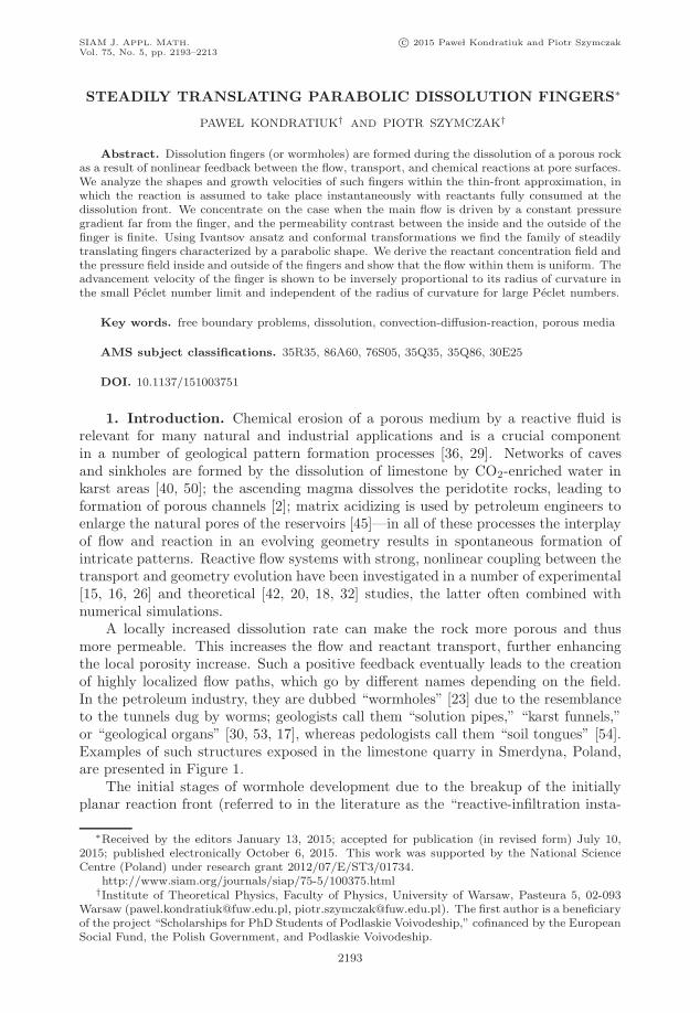
A locally increased dissolution rate can make the rock more porous and thusmore permeable. This increases the flow and reactant transport, further enhancingthe local porosity increase. Such a positive feedback eventually leads to the creationof highly localized flow paths, which go by different names depending on the field.In the petroleum industry, they are dubbed “wormholes” [23] due to the resemblanceto the tunnels dug by worms; geologists call them “solution pipes,” “karst funnels,”or “geological organs” [30, 53, 17], whereas pedologists call them “soil tongues” [54].Examples of such structures exposed in the limestone quarry in Smerdyna, Poland,are presented in Figure 1.

The initial stages of wormhole development due to the breakup of the initiallyplanar reaction front (referred to in the literature as the “reactive-infiltration insta-

∗Received by the editors January 13, 2015; accepted for publication (in revised form) July 10,2015; published electronically October 6, 2015. This work was supported by the National ScienceCentre (Poland) under research grant 2012/07/E/ST3/01734.

http://www.siam.org/journals/siap/75-5/100375.html†Institute of Theoretical Physics, Faculty of Physics, University of Warsaw, Pasteura 5, 02-093

Warsaw ([email protected], [email protected]). The first author is a beneficiaryof the project “Scholarships for PhD Students of Podlaskie Voivodeship,” cofinanced by the EuropeanSocial Fund, the Polish Government, and Podlaskie Voivodeship.

2193

c© 2015 Pawe�l Kondratiuk and Piotr Szymczak

http://www.siam.org/journals/siap/75-5/100375.html

mailto:[email protected]

mailto:[email protected]

2194 PAWE�L KONDRATIUK AND PIOTR SZYMCZAK

Fig. 1. Solution pipes in the limestone quarry in Smerdyna (Poland), formed in limestonebedrock. They are postulated to have been formed by a dissolving action of meltwater during Elsteriandeglaciation [37, 53]. The brown rims in the clay filling the pipes are the result of clay and ironoxide accumulation due to the illuviation processes [47]. The clay particles are transferred by waterfrom the upper parts of the soil and then flocculated at the clay-limestone boundary, where the pHchanges from mildly acidic to alkaline.

bility”) have been extensively studied [8, 39, 48, 9, 22, 52] and are now quite wellunderstood. Much less is known, however, about the nonlinear regime, when theinitial perturbations of the interface are transformed into finger-like structures thatadvance into the system [15, 21, 41, 11, 49]. An important question in this contextconcerns the existence of a self-preserving form that might model the growing tip.Such invariantly propagating forms have been found in other pattern forming sys-tems, e.g., the Saffman–Taylor finger in viscous fingering or the Ivantsov paraboloidin dendritic growth [46, 24, 28, 1, 14]. Our goal in this paper is to find such solutionsfor a dissolving porous medium.

In the context of dissolution, the propagation of individual fingers was studiedin petroleum engineering [27, 6, 11]. In these works, simple geometric models ofwormhole shapes were adopted, which are not preserved during the growth. Theclosest in spirit to the present study is the work by Nilson and Griffiths [38]. Theytackle the problem of steadily propagating dissolution forms and find them to beparabolic (in two dimensions) or paraboloidal (in three dimensions). However, thereare significant differences between their approach and the present one. We discussthose in more detail in section 5. Here we will just note that in [38] the reactantconcentration field is not resolved; instead the dissolution front velocity is taken tobe proportional to the local fluid velocity. Additionally, the pressure drop inside thefinger is neglected, which is only justified if the permeability of the dissolved phaseis much higher than the permeability of the primary rock. In that way, the problemis effectively reduced to a one-phase problem, requiring the solution of the Laplaceequation for pressure in the region outside the finger only. As discussed in [25, 12]such “one-phase” growth problems are in general much easier to solve than the “two-phase” problems in which the flow fields both inside and outside the finger need tobe found, which is also the case in the present study. On top of this, to find the


STEADILY TRANSLATING PARABOLIC DISSOLUTION FINGERS 2195

Fig. 2. Geometry of the system: a reactive fluid is injected from the left and dissolves theporous matrix through chemical reactions. In the course of dissolution, the reaction front, shownby the solid line, advances into the matrix (dashed line), separating the dissolved, upstream domain(Ω) of porosity φ1 and the undissolved, downstream domain (Ω) of porosity φ0, complementary toΩ.

finger advancement velocity, we need to solve not only for the pressure, but also forthe reactant concentration field, which makes the task at hand more challenging.

The paper is organized as follows. In section 2 the general equations governingthe dynamics of the dissolving porous rock are briefly recalled and then put in di-mensionless form in section 3. The core of the paper is sections 4 and 6, where, afterthe application of the Ivantsov ansatz, we obtain the family of steadily translatingdissolution fingers and show that they are parabolic/paraboloidal. Let us reiteratethat despite a formal similarity to the Ivantsov forms, the physics of growth is quitedifferent here, as it involves an interplay between the flow field and solute concen-tration field in contrast to the dendritic growth which is controlled by a single field(temperature only).

2. The model of matrix dissolution. When a porous matrix is infiltrated byan incoming flux of reactive fluid, a front develops once all the soluble material atthe inlet has been dissolved. This front propagates into the matrix, as illustrated inFigure 2. Upstream of the front, all the soluble material has dissolved and the porosityis constant, φ = φ1. Ahead of the front, the porosity decays gradually to its value inthe undissolved matrix, φ = φ0. The front is initially planar but eventually breaksup because of a positive feedback between flow and dissolution, which amplifies anysmall variations in the porosity field [8].

Let us briefly recall the equations for the dissolution of a porous matrix. Rateof groundwater flow through the porous medium is taken to be proportional to thepressure gradient (Darcy’s law),

(2.1) v = −K∇p

μ,

where v is the Darcy velocity, φ is the porosity, and K(φ) is the permeability. Wealso assume that the Darcy velocity field is incompressible,

(2.2) ∇ · v = 0,

neglecting contributions to the fluid volume from reactants or dissolved products.Under typical geophysical conditions, dissolution is slow in comparison to flow andtransport processes; we can therefore assume a steady state in both the flow andtransport equations.



The transport of reactants is described by a convection-diffusion-reaction equa-tion,

(2.3) ∇ · (vc) −∇ · (Dφ∇c) = −R,

where c denotes the concentration of the reactant, and R(c) is the reactive flux intothe matrix. In the upstream region, where all the soluble material has dissolved (φ =φ1), the reaction term vanishes and the transport equation reduces to a convection-diffusion equation.

In the derivations below, we adopt a thin-reaction-front approximation, in whichthe transition zone over which the porosity changes is assumed to be infinitely thin[8, 39]. As shown in [51], this approximation is applicable whenever the reactantpenetration length is short in comparison with the diffusive length scale D/v, char-acterizing the decay of the concentration in the upstream region. In practice, thishappens whenever the parameter H = Dk/v2 � 1 [51], where k is the dissolutionrate (assuming the first order reaction kinetics); thus the reaction rate needs to besufficiently high and/or the flow rate sufficiently low. As a consequence, we obtaina Stefan-like problem in which the space is divided into two domains: the dissolved,upstream domain (Ω) of porosity φ1 and the undissolved, downstream domain (Ω)of porosity φ0, complementary to Ω. The reaction front (∂Ω) advances with velocityproportional to the flux of the reactant at a given point

(2.4) Un = − γ

cinD (∇c)n ,

where subscript n represents the component normal to the interface, cin is the inletconcentration of the reactant, and the acid capacity number γ = cin/νcsol(φ1 − φ0)is defined as the volume of rock (of molar concentration csol) that is completelydissolved by a unit volume of reactant (of molar concentration cin). Finally, ν is thestoichiometric coefficient in the dissolution reaction (number of moles of the reactantnecessary to dissolve one mole of the rock).

The flux of reactant in (2.4) is taken to be purely diffusive, since the thin-frontapproximation implies vanishing of c at the interface, as it is fully consumed there:

(2.5) c|∂Ω(t) = 0.

Because in both domains the porosity (and hence permeability) is constant, (2.1)–(2.2) can be combined to yield the Laplace equation for the pressure

(2.6) ∇2p = 0

in both Ω and Ω.The above equations are supplemented by boundary conditions on the velocity

and concentration field as x → ∞:

v(x → ∞) = v0ex, c(x → ∞) = 0,(2.7)

which account for the fact that far from the dissolution front the flow becomes uniformand the reactant concentration vanishes. The conditions at x → −∞ are somewhatmore subtle. If the reaction front assumes such a form that sufficiently far upstreameverything is dissolved, i.e., ∃x0 (∀x < x0, (x, y) ∈ Ω), then it is possible to impose

(2.8) ∂xvx(x → −∞) = 0



on the flow field and

(2.9) c(x → −∞) = cin

on the concentration field, the former representing the condition that the flow becomesuniform far upstream, the latter corresponding to the reactant concentration imposedat the inlet.

However, if the undissolved phase (Ω) extends toward x → −∞ (as is the case fora solitary dissolution finger surrounded by an undissolved matrix), then the conditionanalogous to (2.9) should be imposed only within the finger, and not on the entirex → −∞ line. We will come back to this issue later on.

Additionally, both the pressure and the normal component of the Darcy velocityneed to be continuous across the reaction front ∂Ω:

p|∂Ω(t)− = p|∂Ω(t)+ ,(2.10)

vn|∂Ω(t)− = vn|∂Ω(t)+ .(2.11)

3. Scaling of the variables and the limiting cases. The dissolution equa-tions (2.1)–(2.3) can be simplified by scaling the velocity, concentration, and porosityfields by their characteristic values

(3.1) v = v/v0, c = c/cin, φ =φ− φ0

φ1 − φ0,

where the scaled, dimensionless variables are marked by hats. Additionally, we scalethe spatial coordinates by some length l, characterizing the wormhole, and time byτ = l/γv0. Using l, we can scale the pressure as follows:

(3.2) p =K(φ0)

v0μlp.

With these scalings, the governing equations take the form

∇2p = 0, r ∈ Ω(t),(3.3)

κ∇p · ∇c + Pe −1∇2c = 0, r ∈ Ω(t),(3.4)

in the upstream region and

∇2p = 0, r ∈ Ω(t),(3.5)

c = 0, r ∈ Ω(t),(3.6)

in the downstream one. In the above,

(3.7) Pe ≡ v0l

φ1D(φ1)

is the Peclet number which measures the relative magnitude of convective and diffusiveeffects on the length scale l, whereas

(3.8) κ ≡ K(φ1)

K(φ0)



is the ratio of permeability between the domains. In typical geological conditionsthe permeability is an increasing function of porosity, thus κ > 1. The boundaryconditions (2.7)–(2.9) in the scaled variables take the form

v(x → ∞) = ex, c(x → ∞) = 0(3.9)

and

(∂xvx)(x → −∞) = 0, c(x → −∞) = 1,(3.10)

which, as before, need to be supplemented by the continuity conditions for the pressurep and the normal component of the velocity vn across the interface1 at the boundary(reaction front) ∂Ω. Finally, the condition (2.4) for the front advancement velocitytakes the form

(3.11) Un = −Pe−1(∇c)n.

Noting that at the reaction front the concentration satisfies

(3.12) U · ∇c +∂c

∂t= 0,

one can rewrite (3.11) in terms of c only:

(3.13)∂c(r)

∂t− Pe −1|∇c(r)|2 = 0, r ∈ ∂Ω(t).

It is relatively straightforward to derive the one-dimensional solutions of (3.3)–(3.6), corresponding to the planar reactive front propagating with a constant velocity,U0. Assuming that both c and p are the functions of only x leads to

(3.14) p(x) =

{ −κ−1x, x < 0,−x, x > 0,

where x = x− U0t is the coordinate moving with the front. For the concentration weget an exponentially decaying, diffusive profile:

(3.15) c(x) =

{1 − ePe x, x < 0,0, x > 0.

Finally, inserting the above into the front velocity condition (3.11), we obtain theresult U0 = 1; i.e., in the units chosen the planar reaction front advances with a unitvelocity along the flow direction.

4. Stationary dissolution fingers in two dimensions. In this section, wederive the shape of a single dissolution finger propagating invariantly toward theundissolved matrix. We begin with the two-dimensional case.

At the boundary between the phases, (3.13) is satisfied. Without any loss ingenerality, one might extend this equation to the whole domain Ω as

(4.1) F (r, t)∂c

∂t− |∇c|2 = 0,

1Note that v = −κ∇p on Ω and v = −∇p on Ω.



with F formally given as F = |∇c|2/∂tc and satisfying F |r∈∂Ω(t) = Pe . To proceed,

we use the ansatz due to Ivantsov [28, 1] by assuming that the unknown F functiondependence on the spatial and time coordinates is of the form

(4.2) F (r, t) = F (c(r, t)),

so that

(4.3) F (c)∂c

∂t− |∇c|2 = 0

is satisfied in the whole domain Ω. Obviously, F must satisfy

(4.4) F (c = 0) = Pe

for consistency with the boundary condition (3.13). Using this idea, Ivantsov hasfound his famous set of steady-state solutions to the dendrite growth problem in asupercooled melt. Note that assuming the ansatz (4.2) might lead to losing some ofthe more general solutions of the problem.

Let us now suppose that our problem has a stationary solution: a dissolutionfinger moving invariantly in the x direction with velocity U . Rewriting (4.3) in themoving coordinate system gives

(4.5) −UF (c)∂c

∂x− |∇c|2 = 0

or

(4.6) ∇c · (∇c + UF (c)∇x) = 0.

Let us note that both the Laplace equation (3.3) and the advection-diffusion equa-tion with potential flow (3.4) are conformally invariant. A large class of conformallyinvariant, non-Laplacian physical problems has been identified by Bazant in [3, 4]and involves such phenomena as nonlinear diffusion or advection or electromigrationcoupled to diffusion. The conformal invariance of these processes provides an effec-tive way of solving these problems [10]. In the context of growth processes, thesetechniques have been used to track the evolution of the interface in solidification andmelting under the action of a potential flow [34, 19, 33, 14, 13, 3, 5]. However, in theseworks growth has been taking place in external flows (with the fluid outside of thegrowing object), in contrast to the present case where the medium is porous, and thedriving flow goes through the growing finger and then into the undissolved medium.

In our case, (4.6) is also written in a conformally invariant form. This allows usto make a conformal coordinate transformation (x, y) → (ξ, η) such that c = c(ξ) (i.e.,the isolines of c coincide with the curves ξ(x, y) = const). Since (4.6) is conformallyinvariant, we get

(4.7)dc

dξ+ UF (c(ξ))

∂x

∂ξ= 0.

The immediate conclusion is that ∂x∂ξ must be a function of ξ only,2 hence

(4.8) x(ξ, η) = Φ1(ξ) + Φ2(η).

2Note that if one sought a stationary solution without having assumed the Ivantsov ansatz, onewould obtain at this point

dc

dξ+ UF (ξ, η)

∂x

∂ξ= 0,

which does not provide any information about the mapping.



The Cauchy–Riemann conditions,

(4.9)∂y

∂η=

∂x

∂ξ,

∂y

∂ξ= −∂x

∂η,

lead to the Laplace equation for x, ∇2ξηx = 0, the general solution of which, compatible

with (4.8), is

(4.10a) x(ξ, η) =1

2ρ((ξ − ξ∗)2 − (η − η∗)2

).

Using again (4.9) allows us to find y(ξ, η) in the form

(4.10b) y(ξ, η) = ρ(ξ − ξ∗)(η − η∗) + y∗.

Without loss of generality we can set ξ∗ = η∗ = y∗ = 0. Furthermore, we can assumethat the parabola characterized by ξ = 1 corresponds to the dissolution front (anyother parabola can be scaled onto it by an appropriate choice of parameter ρ). Notethat the parameter ρ corresponds to the (dimensionless) radius of curvature of theparabolic finger. This suggests that the (dimensional) radius of curvature, ρ, couldbe used as a length parameter in our problem. Taking l = ρ leads to ρ = 1, whichsimplifies the subsequent analysis.

Our final conclusion is the following: the only conformal mapping (x, y) → (ξ, η)which makes the concentration field in the dissolution finger a function of one variableonly, c(x, y) = c(ξ(x, y)), is (up to translation)3

x(ξ, η) =1

2

(ξ2 − η2

),(4.11)

y(ξ, η) = ξη,(4.12)

which is the usual transformation to the parabolic coordinates.It is worth noting that parabolic geometries have also been obtained by other au-

thors studying steadily translating growth forms. The classical example is Ivantsov’sdendrites [28]. In fact, Adda-Bedia and Ben Amar [1] have shown that, at least in thecontext of steady-state dendritic growth at zero surface tension, the parabolic solu-tions are the only admissible solutions once the Ivantsov ansatz is adopted and thateven when one modifies this approach by making a more general ansatz, no new formsare found. Although the present case is of a more complicated nature, it is possiblethat also here the adoption of the Ivantsov ansatz necessitates the appearance of theparabolic forms.

Once the shape of the finger is known, we can find the concentration and pressureboth inside and outside of it.

4.1. Solution inside the finger. Inside the dissolution finger (i.e., for ξ < 1)

Peκ∂p

∂ξ

dc

dξ+

d2c

dξ2= 0,(4.13)

∂2p

∂ξ2+

∂2p

∂η2= 0,(4.14)

dc

dξ+ UF (c(ξ))

∂x

∂ξ= 0.(4.15)

3In fact, we also assume the Ivantsov ansatz (equation (4.3)).



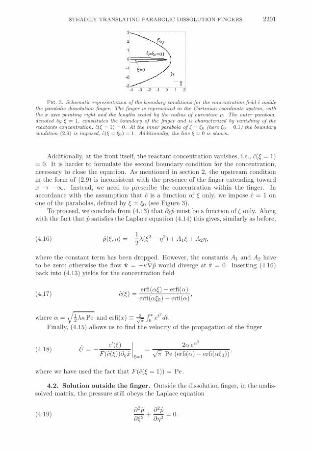
Fig. 3. Schematic representation of the boundary conditions for the concentration field c insidethe parabolic dissolution finger. The finger is represented in the Cartesian coordinate system, withthe x axis pointing right and the lengths scaled by the radius of curvature ρ. The outer parabola,denoted by ξ = 1, constitutes the boundary of the finger and is characterized by vanishing of thereactants concentration, c(ξ = 1) = 0. At the inner parabola of ξ = ξ0 (here ξ0 = 0.1) the boundarycondition (2.9) is imposed, c(ξ = ξ0) = 1. Additionally, the line ξ = 0 is shown.

Additionally, at the front itself, the reactant concentration vanishes, i.e., c(ξ = 1)= 0. It is harder to formulate the second boundary condition for the concentration,necessary to close the equation. As mentioned in section 2, the upstream conditionin the form of (2.9) is inconsistent with the presence of the finger extending towardx → −∞. Instead, we need to prescribe the concentration within the finger. Inaccordance with the assumption that c is a function of ξ only, we impose c = 1 onone of the parabolas, defined by ξ = ξ0 (see Figure 3).

To proceed, we conclude from (4.13) that ∂ξp must be a function of ξ only. Alongwith the fact that p satisfies the Laplace equation (4.14) this gives, similarly as before,

(4.16) p(ξ, η) = −1

2λ(ξ2 − η2) + A1ξ + A2η,

where the constant term has been dropped. However, the constants A1 and A2 haveto be zero; otherwise the flow v = −κ∇p would diverge at r = 0. Inserting (4.16)back into (4.13) yields for the concentration field

(4.17) c(ξ) =erfi(αξ) − erfi(α)

erfi(αξ0) − erfi(α),

where α =√

12λκPe and erfi(x) ≡ 2√

π

∫ x

0et

2

dt.

Finally, (4.15) allows us to find the velocity of the propagation of the finger

(4.18) U = − c′(ξ)

F (c(ξ))∂ξx

∣∣∣∣ξ=1

=2α eα

2

√π Pe (erfi(α) − erfi(αξ0))

,

where we have used the fact that F (c(ξ = 1)) = Pe .

4.2. Solution outside the finger. Outside the dissolution finger, in the undis-solved matrix, the pressure still obeys the Laplace equation

(4.19)∂2p

∂ξ2+

∂2p

∂η2= 0.



The continuity conditions for p and the vn ≡ vξ yield here

−1

2λ(1 − η2) = p|ξ→1+ ,(4.20)

−κλ =∂p

∂ξ

∣∣∣∣ξ→1+

.(4.21)

This is supplemented by the boundary condition (2.7)

(4.22) −∇p∣∣∣ξ→∞

= ex = ∇x,

which can be written in the (ξ, η) coordinates as

(4.23) limξ→∞

1

ξ

∂p

∂ξ= −1, lim

ξ→∞1

η

∂p

∂η= 1.

The solution of (4.19) fulfilling (4.20)–(4.23) is

(4.24) p(ξ, η) = −1

2(ξ2 − η2) − (κ− 1)(ξ − 1).

Additionally, the condition (4.21) gives λ = 1 for the constant appearing in thesolution of the internal problem ( 4.16)–(4.17).

4.3. Summary. The pressure field in the system is

(4.25) p(ξ, η) =

{− 1

2 (ξ2 − η2) for 0 ≤ ξ ≤ 1,

− 12 (ξ2 − η2) − (κ− 1)(ξ − 1) for ξ ≥ 1.

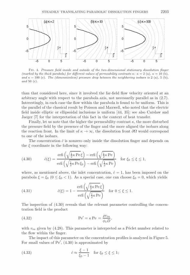
Figure 4 shows the pressure fields, plotted for various permeability contrasts κ, in thephysical (x, y) plane. Note that inside the finger the isobars are parallel to each otherand oriented along the y direction, which is a manifestation of the fact that the flowis uniform there:

p(x, y) = −x, r ∈ Ω,(4.26)

v(x, y) = κex, r ∈ Ω.(4.27)

In the dimensional variables, the (constant) Darcy velocity inside the finger is

(4.28) vin = κv0ex.

Outside the finger, in the undissolved domain Ω, the pressure field is

(4.29) p(x, y) = −x− (κ− 1)(√

r + x− 1).

The term linear in x dominates far from the boundary ∂Ω, which agrees with thefar-downstream condition for the flow field (2.7). Note that both the pressure fieldinside the finger (4.27) as well as that outside (4.29) obey the upstream boundarycondition (2.8).

The above-obtained pressure field is analogous to that derived by Kacimov andObnosov [31], who have been analyzing the groundwater flow in a porous mediumwith a parabolic inclusion. In fact the pressure problem solved in [31] is more general



Fig. 4. Pressure field inside and outside of the two-dimensional stationary dissolution finger(marked by the thick parabola) for different values of permeability contrasts κ: κ = 2 (a), κ = 10 (b),and κ = 100 (c). The (dimensionless) pressure drop between the neighboring isobars is 2 (a), 5 (b),and 50 (c).

than that considered here, since it involved the far-field flow velocity oriented at anarbitrary angle with respect to the parabola axis, not necessarily parallel as in (2.7).Interestingly, in each case the flow within the parabola is found to be uniform. This isthe parallel of the classical result by Poisson and Maxwell, who noted that the electricfield inside elliptic or ellipsoidal inclusions is uniform [44, 35]; see also Carslaw andJaeger [7] for the interpretation of this fact in the context of heat transfer.

Finally, let us note that the higher the permeability contrast κ, the more disturbedthe pressure field by the presence of the finger and the more aligned the isobars alongthe reaction front. In the limit of κ → ∞, the dissolution front ∂Ω would correspondto one of the isobars.

The concentration c is nonzero only inside the dissolution finger and depends onthe ξ coordinate in the following way:

(4.30) c(ξ) =erfi

(√12κPe ξ

)− erfi

(√12κPe

)erfi

(√12κPe ξ0

)− erfi

(√12κPe

) for ξ0 ≤ ξ ≤ 1,

where, as mentioned above, the inlet concentration, c = 1, has been imposed on theparabola ξ = ξ0 (0 ≤ ξ0 < 1). As a special case, one can choose ξ0 = 0, which yields

(4.31) c(ξ) = 1 −erfi

(√12κPe ξ

)erfi

(√12κPe

) for 0 ≤ ξ ≤ 1.

The inspection of (4.30) reveals that the relevant parameter controlling the concen-tration field is the product

(4.32) Pe′ = κPe =ρvinφ1D

,

with vin given by (4.28). This parameter is interpreted as a Peclet number related tothe flow within the finger.

The impact of this parameter on the concentration profiles is analyzed in Figure 5.For small values of Pe′, (4.30) is approximated by

(4.33) c ≈ ξ − 1

ξ0 − 1for ξ0 ≤ ξ ≤ 1;



' ' '

Fig. 5. Reactant concentration field c inside the two-dimensional stationary dissolution finger(marked by the thick parabola) for Pe′ = 0.1 (a), Pe′ = 5 (b), and Pe′ = 10 (c). The boundarycondition for the concentration (2.9) has been imposed on the line ξ = ξ0 = 0. The (dimensionless)concentration drop between the neighboring isolines of c (thin parabolas) is set to 0.1. The boundaryof the finger is also an isoline of the concentration (c = 0).

i.e., the concentration depends linearly on the parabolic coordinate ξ. The gradient ofthe concentration field is then relatively uniform (cf. Figure 5(a)). This situation canbe referred to as the “diffusive” regime. In the opposite case of large Pe′ (the “convec-tive” regime), the concentration boundary layer is formed, with uniform concentrationc = 1 in the body of the finger and high gradients near the boundary (Figure 5(c)). Inthis limit the solutions found by us acquire direct physical relevance since a somewhatartificial choice of ξ0 becomes irrelevant here, as long as the parabola ξ = ξ0 lies in

the bulk. The characteristic width of the boundary layer is(12Pe′

)−1/2; therefore the

condition

(4.34) ξ0 � 1 −(

1

2Pe′

)− 12

guarantees that ξ0 lies in the bulk, and thus its precise value does not affect theconcentration profiles. This is confirmed by the comparison of c profiles for Pe′ = 10and ξ0 = 0.05 with those for ξ0 = 0.2, which are found to be almost indistinguishable,as shown in Figure 6.

Finally, the advancement velocity of the dissolution finger is

(4.35) U = − c′(ξ)

F (c(ξ))∂ξx

∣∣∣∣ξ=1

=

√2κ exp

(12Pe′

)√π Pe′

(erfi

(√12Pe′

)− erfi

(√12Pe′ξ0

)) ,with the two limiting cases (corresponding to small/high values of Pe′) given by

limPe′→0

Pe′U = κ(1 − ξ0)−1,(4.36)

limPe′→∞

U = κ.(4.37)

The velocity scale is l/τ = γv0. Thus in the limit of small Pe′, the dimensional fingeradvancement speed approaches

(4.38) U ≈ γv0κ

Pe′(1 − ξ0)=

γφ1D

ρ(1 − ξ0);



''

' '

Fig. 6. (a), (b) Reactant concentration field c inside the two-dimensional stationary dissolutionfinger in the “convective” regime, with Pe′ = 10. The thick solid lines mark the finger boundary andthe ξ = ξ0 parabola with ξ0 = 0.05 (a) and ξ0 = 0.2 (b), on which the inlet concentration has beenimposed, c(ξ = ξ0) = 1. The (dimensionless) concentration drop between the neighboring isolines ofc (thin parabolas) is set to 0.1. The dashed line marks the parabola η = 2 (locally orthogonal to theisolines of concentration) parametrized by the arc length s. The reactant concentration profile alongthis parabola, c(s), is plotted in panels (c) and (d).

i.e., it is inversely proportional to the radius of curvature of the tip. Such behavioris in full analogy to the Ivantsov result for the dendrite propagation speed [28]. Onthe contrary, for large Peclet numbers the propagation velocity becomes constant withrespect to the curvature of the finger tip and simply proportional to the Darcy velocityinside the finger

(4.39) U ≈ γv0κ = γvin.

Notice the inherent indeterminacy of the general result (4.35): we have obtained therelation between the tip radius and the propagation speed with no means of evaluatingeach of these quantities independently. This is connected with the scale invariance ofthe original equations (2.1)–(2.4) and can be lifted only after the introduction of anadditional length scale. Again, this feature is shared by both the Ivantsov parabolasand the Saffman–Taylor fingers, which also represent families of growth forms andneed the short-scale regularization mechanism such as surface tension or kinetic under-cooling for the selection of a particular tip radius and advancement velocity. In thecase of dissolution patterns, the additional length scale might originate from thereaction front width (assumed to be zero in our analysis) or from the interactionswith other dissolution fingers: in a real system, the finger is never infinite, but alwaysconstrained by the presence of its neighbors.



5. Comparison with the Nilson and Griffiths model. At this point it isworth noting the main differences between our finger growth model and that of Nil-son and Griffiths [38]. First of all, we differ in the boundary conditions at infinity.Whereas we assume that the entire system is flushed with a reactive fluid (with con-stant pressure gradient both at x → −∞ and x → ∞), Nilson and Griffiths assumeconstant pressure at x → ∞, which means that the fluid far from the tip of the fingeris kept immobile. Since at the same time the reactive fluid is constantly injected intothe system, displacing the original pore fluid, the latter becomes compressed, whichdoes not seem to be a realistic assumption under typical groundwater pressures. Inanother case considered in [38] the medium is supposed to be initially unsaturated,with no fluid present. Then the reactive fluid is injected into the the system, creat-ing a finger and flooding the medium in front of the finger tip, forming a “productlayer.” Due to the absence of imposed pressure gradient, the fluid in the productlayer gradually slows down, as the thickness of the layer is increased until it reachesa stationary situation in which both the finger and the product layer advance withequal speeds into the medium. Again, this is a fundamentally different situation fromthe one considered in the present work, where the entire medium is flushed with areactive fluid due to the imposed pressure gradient. In particular, the solution tubesof Figure 1 are formed under such conditions, with the gravity imposing the pressuregradient across the entire system.

There is yet another difference between our approaches, this time related tothe constraints on the values of the physical parameters, under which the fingermodel is supposed to work. Similarly to us, Nilson and Griffiths adopt the thin-front approximation, stating that the reactant is entirely consumed as soon as it hitsthe finger boundary. As mentioned above, this corresponds to the assumption thatH = Dk/v2in � 1. At the same time, however, it is assumed in [38] that the concentra-tion of the reactant inside the finger is constant, so that the dissolution front velocityis proportional to the local fluid velocity. This is only possible if the advection withinthe finger dominates over the diffusive transport, i.e., Pe′ = vinl/D � 1. The doublelimit (Dk/v2in � 1, vinl/D � 1) puts rather stringent constraints on the admissiblevalues of D, vin, and k—i.e., the flow rates should on one hand be large (to keep thetransport advective within the finger), but on the other hand small enough to keepthe reaction front thin. Conversely, in the present work, while keeping the front thin,we fully resolve the concentration field inside the finger, and thus obtain the fingerpropagation velocities over the entire range of Peclet numbers; cf. (4.35). At smallerPe′, effects connected with the buildup of a diffusive layer of the depleted reactantappear [51], which have a significant impact on the wormhole propagation speed.

The differences in the boundary conditions between our system and that of [38]are reflected in different relations between the finger advancement velocity and its tipcurvature. Nilson and Griffiths find that the finger velocity is inversely proportionalto its radius of curvature. We get a similar result, but in the limit of small Pe′ only,when the diffusive effects play a central role in the dynamics. These effects are absentaltogether in the Nilson and Griffiths model. Conversely, we find that for large Pe′

the finger propagation velocity is independent of its curvature.

6. Stationary dissolution fingers in three dimensions. In this section westudy the geometry of three-dimensional dissolution fingers. Again, we assume theIvantsov ansatz as well as the stationarity of the fingers, so the starting point of ourinvestigations is the following set of equations for pressure and concentration inside



the finger:

κ∇p · ∇c + Pe −1∇2c = 0,(6.1a)

∇2p = 0,(6.1b)

∇c · (F (c) U ∇z + ∇c) = 0,(6.1c)

where we have assumed the flow along the z direction. As before, on the boundaryof the finger (ξ = 1) we put c = 0 and F = Pe . In the region outside the finger thepressure obeys the Laplace equation, whereas the concentration vanishes.

Let us switch to the cylindrical coordinate system, (x, y, z) → (r, ϕ, z), and lookfor the solutions with rotational invariance, i.e., independent of ϕ. Equations (6.1) inthe new variables take the form

κPe ∇rz p · ∇rz c + ∇2rz c +

1

r

∂c

∂r= 0, r ∈ Ω(t),(6.2a)

∇2rz p +

1

r

∂p

∂r= 0, r ∈ Ω(t),(6.2b)

∇rz c · (F (c) U ∇rz z + ∇rz c) = 0, r ∈ Ω(t),(6.2c)

where ∇rz = (∂r, ∂z) acts as if the (r, z) were Cartesian coordinates. Similarly,∇2

rz = ∂2r + ∂2

z . Analogously to the previous case, we are looking for a conformal map(z, r) → (ξ, η) such that c becomes a function of one variable only, c = c(ξ). Again,from (6.2c) we draw the conclusion that such a map needs to be a parabolic one,

z =1

2(ξ2 − η2),(6.3a)

r = ξη,(6.3b)

with the radius of curvature of the finger chosen as the unit length. As before, weassume that the finger boundary coincides with the ξ = 1 paraboloid.

Let us now use this mapping to solve the Laplace equation for the pressure in-side and outside of the dissolution finger. Since the Lame coefficients Lξ, Lη for thetransformation (6.3) are equal to

(6.4) Lξ = Lη =

√(∂r

∂ξ

)2

+

(∂z

∂ξ

)2

=√ξ2 + η2,

equation (6.2a) written in terms of ξ and η becomes

(6.5) Pe′∂p

∂ξc′(ξ) + c′′(ξ) +

1

ξc′(ξ) = 0.

Its form suggests that ∂ξp is a function of ξ only, and thus the pressure field p insidethe dissolution finger can be separated into

(6.6) p(ξ, η) = X(ξ) + Y (η).

The Laplace equation for the pressure inside the dissolution finger, (6.2b), in the ξ, ηcoordinates transforms into

(6.7)∂2p

∂ξ2+

∂2p

∂η2+

1

ξ

∂p

∂ξ+

1

η

∂p

∂η= 0, 0 ≤ ξ < 1.



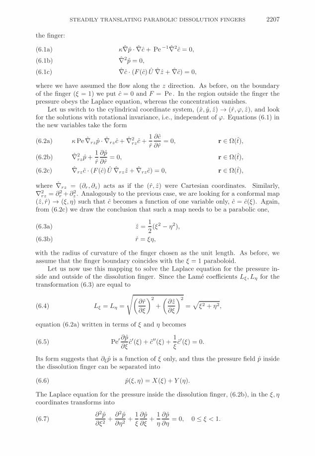
Fig. 7. Pressure field inside and outside of the three-dimensional stationary dissolution finger.The xz cross-section of the finger is shown, with the finger boundary marked by a thick parabola.The pressure field is plotted for different values of permeability contrast: κ = 2 (a), κ = 10 (b), andκ = 100 (c). The (dimensionless) pressure drop between the neighboring isobars is 2 (a), 2.5 (b),and 10 (c).

Inserting (6.6) into (6.7) gives the result that the pressure field inside the dissolutionfinger should be of the form

(6.8) p(ξ, η) = −1

2λ1(ξ2 − η2) + C1 ln ξ + C2 ln η + C3, 0 ≤ ξ < 1.

We set C1 = C2 = 0 to avoid singularities at ξ = 0 or η = 0, while the constants λ1

and C3 are to be determined from the boundary and the continuity conditions. Next,we look for the solution of the Laplace equation for the pressure field outside of thefinger of the same functional form as that inside,

(6.9) p(ξ, η) = −1

2λ2(ξ2 − η2) + D1 ln ξ + D2 ln η, ξ > 1,

where the constant term has been skipped. The continuity conditions and the far-downstream boundary condition for the flow are analogous to the two-dimensionalcase (equations (2.7)–(2.11)). The downstream boundary condition yields λ2 = 1.The continuity of the pressure and the normal component of the flux at the fingerboundary ξ = 1 yields D2 = C3 = 0, λ1 = 1, and D1 = 1−κ. Eventually, the pressurefield in the whole space is

(6.10) p(ξ, η) =

{− 1

2 (ξ2 − η2) for 0 ≤ ξ ≤ 1,

− 12 (ξ2 − η2) − (κ− 1) ln ξ for ξ ≥ 1.

This solution has been plotted in Figure 7 for different values of the permeabilitycontrast, κ. The overall picture is similar to that in the two-dimensional case, witha uniform flow inside the finger and the flow disturbance around it relaxing to auniform flow field far downstream. For small values of the permeability contrast κ,the presence of the finger does not significantly disturb the isobars, whereas in theopposite case the isobars become almost parallel to the finger boundary.

Using (6.10) one can solve (6.5) and find the concentration field inside the finger.Formally, the solution can be written in terms of the exponential integral functionEi,4

(6.11) c(ξ) =Ei

(12Pe′ξ2

)− Ei(12Pe′

)Ei

(12Pe′ξ20

)− Ei(12Pe′

) , ξ0 < ξ < 1,

4The exponential integral function is defined as Ei(x) ≡ − ∫∞−x t−1e−tdt.



'' '

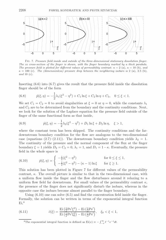
Fig. 8. Reactant concentration field c in the cross-section of the three-dimensional stationarydissolution finger, for Pe′ = 0.1 (a), 10 (b), and 20 (c). The parameter ξ0 was chosen to be 0.1.The (dimensionless) concentration drop between the neighboring isolines is set to 0.1.

where, as before, we set the condition c = 1 on the parabola ξ = ξ0 (with 0 < ξ0 <1). The concentration fields for various parameters have been plotted in Figure 8.Qualitatively, the behavior is similar to that observed for the two-dimensional case.The “diffusive” regime is observed for small values of Pe′ (see Figure 8(a)) and ischaracterized by relatively uniform distribution of the concentration gradient. In thiscase, the concentration field can be approximated by5

(6.12) c(ξ) ≈ ln ξ

ln ξ0, ξ0 < ξ < 1.

In the opposite case of high Pe′ (see Figure 8(c)), the boundary layer characterizedby high gradients of the concentration c is formed near the finger boundary, whilein the interior of the finger the c field is almost uniform. The characteristic widthof the boundary layer in the (ξ, η) plane is, similarly as in the two-dimensional case,(12Pe′

)−1/2, which sets the constraint on the choice of ξ0, analogous to the two-dimensional one (equation (4.34)). The only significant difference between the three-and two-dimensional cases is that in three-dimensional we cannot demand ξ0 = 0,since the Ei function diverges at zero and the solution becomes singular. However,this constraint becomes irrelevant in the “convective” regime (Pe′ � 1), since thenc ≈ 1 throughout the bulk of the finger.

Finally, the finger propagation velocity, derived analogously to the two-dimensionalcase, is given by

(6.13) U = − c′(ξ)

F (c(ξ))∂ξ z

∣∣∣∣ξ=1

=2κ(Pe′)−1 exp

(12Pe′

)Ei

(12Pe′

)− Ei(12Pe′ξ20

) ,with the limiting cases characterized by

limPe′→0

UPe′ = −κ(ln ξ0)−1,(6.14)

limPe′→∞

U = κ.(6.15)

Again, there is a significant similarity with the two-dimensional case. The (dimen-sional) propagation velocity of dissolution fingers at small Peclet numbers is inversely

5Ei(x) = γ + lnx + x + O(x2).



proportional to ρ,

(6.16) U ≈ − κγv0Pe ln ξ0

= − γφ1D

ρ ln ξ0,

whereas at high Peclet numbers the propagation velocity becomes independent of theradius of curvature and yields

(6.17) U ≈ γvin.

7. Summary and conclusions. In this paper, we have been analyzing the ge-ometry of the dissolution fingers, which are commonly found in soluble rocks. Wehave adopted the thin-front approximation, in which the reaction is assumed to takeplace instantaneously with the reactants fully consumed at the dissolution front. Inthis way the problem has become Stefan-like with the undissolved phase downstreamand the fully dissolved phase upstream. In such a setup we have posed the problem ofexistence and shape of steadily growing fingers. Two potentially limiting assumptionshave been made. First, we have adopted the Ivantsov ansatz (4.3), which has beensuccessfully used in other studies of dendritic growth [28, 24, 1], usually leading to theparabolic forms of advancing dendrites. Moreover, we have assumed that the trans-formation (x, y) → (ξ, η) from the original Cartesian coordinates to the coordinatesspanned by the isolines and gradient lines of the reactant concentration field c is con-formal. Both of these assumptions limit the class of solutions that can be found withthis technique, leading, however, to significant simplifications in the analysis, since theIvantsov equation (4.6) is conformally invariant and takes a particularly simple form(4.7) in the new coordinate system, where c = c(ξ). The analysis of these equationsleads to the conclusion that (ξ, η) are parabolic coordinates and thus the advancingfront is also of a parabolic form. The flow within the finger turns out to be uniform, inagreement with the earlier studies on the refraction of groundwater flow on parabolicinclusions [31]. The magnitude of the flow is solely the function of the permeabilityratio between the dissolved and undissolved matrix, κ. The concentration field isalso relatively simple and can be expressed in terms of the imaginary error function(in two dimensions, (4.30)) or the exponential integral (in three dimensions, (6.11)).This time, the parameter controlling the shape of the field lines is Pe′, defined as theratio of convective and diffusive fluxes within the wormhole on the length scale of theradius of curvature of the finger tip.

However, these simplifications come at a price, as we can only impose the con-centration boundary conditions on the ξ = const lines, which limits the usefulness ofthese solutions in the physical applications. The most relevant physically seems tobe the case of large Peclet numbers, since in that case the concentration within thefinger becomes uniform, with the exception of a thin boundary layer at the reactionfront itself, and the exact placement of Dirichlet boundaries becomes irrelevant.

Finally, we have obtained the finger propagation velocity, which turns out to beinversely proportional to the radius of curvature in the small Pe′ limit and constant forlarge Pe′. Interestingly, the former prediction seems to be confirmed by the analysisof the shapes of the solution pipes—the inspection of Figure 1 and other photographsfrom this site reveals that the longer fingers have invariably smaller radii of curvatures.

The scale invariance of the problem leads to the dynamical indeterminacy: anyadvancement velocity is permissible, provided that the radius of curvature of the fingeris appropriately tuned; there is no selection principle to fix the tip curvature and thefinger propagation velocity independently. Finding such a selection principle is in



general a highly nontrivial task [43] and involves introducing an additional lengthscale into the system. In the case of viscous fingering and dendritic growth this isachieved through the short-scale regularization mechanisms such as surface tensionor kinetic undercooling. It is not clear what the physical origin would be of such ashort-scale regularization in the present case. A candidate for the additional lengthscale could be the reaction front width, which in our analysis is zero, but remainsfinite in any physical case. Another possibility is that the additional length scalesought here is connected with the presence of other fingers, as it is always the case innatural systems (cf. Figure 1). The full solution of the problem would then requirematching the solution near the parabolic tip with that in the neighborhood of theroot of the finger, where it joins with its neighbors.

Acknowledgment. The authors benefited from discussions with Tony Ladd andKrzysztof Mizerski.

REFERENCES

[1] M. Adda-Bedia and M. Ben Amar, Investigations on the dendrite problem at zero surfacetension in 2D and 3D geometries, Nonlinearity, 7 (1994), pp. 765–776.

[2] E. Aharonov, J. Whitehead, P. Kelemen, and M. Spiegelman, Channeling instability ofupwelling melt in the mantle, J. Geophys. Res., 100 (1995), pp. 433–455.

[3] M. Bazant, J. Choi, and B. Davidovitch, Dynamics of conformal maps for a class of non-Laplacian growth phenomena, Phys. Rev. Lett., 91 (2003), 045503.

[4] M. Z. Bazant, Conformal mapping of some non-harmonic functions in transport theory, Proc.R. Soc. Lond. Ser. A Math. Phys. Eng. Sci., 460 (2004), pp. 1433–1452.

[5] M. Z. Bazant, Interfacial dynamics in transport-limited dissolution, Phys. Rev. E, 73 (2006),060601.

[6] M. A. Buijse, Understanding wormholing mechanisms can improve acid treatments in carbon-ate formations, SPE Prod. Facilities, 8 (2000), pp. 168–175.

[7] H. S. Carslaw and J. C. Jaeger, Heat in Solids, Clarendon Press, Oxford, 1959.[8] D. Chadam, D. Hoff, E. Merino, P. Ortoleva, and A. Sen, Reactive infiltration instabili-

ties, IMA J. Appl. Math., 36 (1986), pp. 207–221.[9] D. Chadam, P. Ortoleva, and A. Sen, A weakly nonlinear stability analysis of the reactive

infiltration interface, SIAM J. Appl. Math., 48 (1988), pp. 1362–1378.[10] J. Choi, D. Margetis, T. M. Squires, and M. Z. Bazant, Steady advection-diffusion around

finite absorbers in two-dimensional potential flows, J. Fluid Mech., 536 (2005), pp. 155–184.

[11] C. Cohen, D. Ding, M. Quintard, and B. Bazin, From pore scale to wellbore scale: Impactof geometry on wormhole growth in carbonate acidization, Chem. Eng. Sci., 63 (2008),pp. 3088–3099.

[12] D. G. Crowdy, Exact solutions to the unsteady two-phase Hele-Shaw problem, Quart. J. Mech.Appl. Math., 59 (2006), pp. 475–485.

[13] L. J. Cummings and K. Kornev, Evolution of flat crystallisation front in forced hydrodynamicflow–some explicit solutions, Phys. D, 127 (1999), pp. 33–47.

[14] L. M. Cummings, Y. E. Hohlov, S. D. Howison, and K. Kornev, Two-dimensional solidi-fication and melting in potential flows, J. Fluid Mech., 378 (1999), pp. 1–18.

[15] G. Daccord, Chemical dissolution of a porous medium by a reactive fluid, Phys. Rev. Lett.,58 (1987), pp. 479–482.

[16] G. Daccord and R. Lenormand, Fractal patterns from chemical dissolution, Nature, 325(1987), pp. 41–43.

[17] J. De Waele, S.-E. Lauritzen, and M. Parise, On the formation of dissolution pipes inQuaternary coastal calcareous arenites in Mediterranean settings, Earth Surf. Proc. Land.,36 (2011), pp. 143–157.

[18] W. Dreybrodt, The role of dissolution kinetics in the development of karst aquifers in lime-stone: A model simulation of karst evolution, J. Geol., 98 (1990), pp. 639–655.

[19] M. Goldstein and R. Reid, Effect of fluid flow on freezing and thawing of saturated porousmedia, Proc. Roy. Soc. London Ser. A, 364 (1978), pp. 45–73.

[20] F. Golfier, B. Bazin, R. Lenormand, and M. Quintard, Core-scale description of porousmedia dissolution during acid injection - Part I: Theoretical development., Comput. Appl.



Math., 23 (2004), pp. 173–194.[21] F. Golfier, C. Zarcone, B. Bazin, R. Lenormand, D. Lasseux, and M. Quintard, On the

ability of a Darcy-scale model to capture wormhole formation during the dissolution of aporous medium, J. Fluid Mech., 457 (2002), pp. 213–254.

[22] E. J. Hinch and B. S. Bhatt, Stability of an acid front moving through porous rock, J. FluidMech., 212 (1990), pp. 279–288.

[23] M. L. Hoefner and H. S. Fogler, Pore evolution and channel formation during flow andreaction in porous media, AIChE J., 34 (1988), pp. 45–54.

[24] G. Horvay and J. W. Cahn, Dendritic and spheroidal growth, Acta Metall., 9 (1961), pp. 695–705.

[25] S. D. Howison, A note on the two-phase Hele-Shaw problem, J. Fluid. Mech., 409 (2000),pp. 243–249.

[26] J. M. Huang, M. N. J. Moore, and L. Ristroph, Shape dynamics and scaling laws for abody dissolving in fluid flow, J. Fluid Mech., 765 (2015), R3.

[27] K. M. Hung, A. D. Hill, and K. Spehrnoori, A mechanistic model of wormhole growth incarbonate acidizing and acid fracturing, J. Pet. Tech., 41 (1989), pp. 59–66.

[28] G. P. Ivantsov, Temperature field around a spheroidal, cylindrical and acicular crystal growingin a supercooled melt, Dokl. Akad. Nauk SSSR, 58 (1947), pp. 567–569.

[29] B. Jamtveit and P. Meakin, Growth, Dissolution and Pattern Formation in Geosystems,Springer, 1999.

[30] J. N. Jennings, Karst Geomorphology, Blackwell Oxford, 1985.[31] A. R. Kacimov and Y. V. Obnosov, Steady water flow around parabolic cavities and through

parabolic inclusions in unsaturated and saturated soils, J. Hydrol., 238 (2000), pp. 65–77.[32] N. Kalia and V. Balakotaiah, Modeling and analysis of wormhole formation in reactive

dissolution of carbonate rocks, Chem. Eng. Sci., 62 (2007), pp. 919–928.[33] K. Kornev and G. Mukhamadullina, Mathematical theory of freezing for flow in porous

media, Proc. Roy. Soc. London Ser. A, 447 (1994), pp. 281–297.[34] V. Maksimov, On the determination of the shape of bodies formed by solidification of the fluid

phase of the stream, J. Appl. Math. Mech., 40 (1976), pp. 264–272.[35] J. C. Maxwell, A Treatise on Electricity and Magnetism, Vol. 2, Clarendon Press, Oxford,

1881.[36] P. Meakin and B. Jamtveit, Geological pattern formation by growth and dissolution in aque-

ous systems, Proc. Roy. Soc. London Ser. A, 466 (2010), pp. 659–694.[37] I. Morawiecka and P. Walsh, A study of solution pipes preserved in the miocene limestones

(Staszow, Poland), Acta Carsologica, 25 (1997), pp. 337–350.[38] R. H. Nilson and S. K. Griffiths, Wormhole growth in soluble porous materials, Phys. Rev.

Lett., 65 (1990), pp. 1583–1586.[39] P. Ortoleva, J. Chadam, E. Merino, and A. Sen, Geochemical self-organization II: The

reactive-infiltration instability, Amer. J. Sci., 287 (1987), pp. 1008–1040.[40] A. N. Palmer, Origin and morphology of limestone caves, Geol. Soc. Amer. Bull., 103 (1991),

pp. 1–21.[41] M. Panga, M. Ziauddin, and V.Balakotaiah, Two-scale continuum model for simulation of

wormhole formation in carbonate acidization, AIChE J., 51 (2005), pp. 3231–3248.[42] A. Pawell and K.-D. Krannich, Dissolution effects in transport in porous media, SIAM J.

Appl. Math., 56 (1996), pp. 89–118.[43] P. Pelce, New Visions on Form and Growth: Fingered Growth, Dendrites, and Flames,

Oxford University Press, 2004.[44] S.-D. Poisson, Second memoire sur la theorie du magnetisme, Memoires Paris Acad. Sci., 5

(1826), pp. 488–533,[45] G. Rowan, Theory of acid treatment of limestone formations, J. Inst. Pet., 45 (1959), pp. 321–

334.[46] P. G. Saffman and G. Taylor, The penetration of a fluid into a porous medium or Hele-

Shaw cell containing a more viscous liquid, Proc. Roy. Soc. London. Ser. A, 245 (1958),pp. 312–329.

[47] R. Schaetzl and S. Anderson, Soils: Genesis and Geomorphology, Cambridge UniversityPress, 2005.

[48] J. D. Sherwood, Stability of a plane reaction front in a porous medium, Chem. Eng. Sci., 42(1987), pp. 1823–1829.

[49] P. Szymczak and A. J. C. Ladd, Wormhole formation in dissolving fractures, J. Geophys.Res., 114 (2009), B06203.

[50] P. Szymczak and A. J. C. Ladd, The initial stages of cave formation: Beyond the one-dimensional paradigm, Earth Planet. Sci. Lett., 301 (2011), pp. 424–432.



[51] P. Szymczak and A. J. C. Ladd, Interacting length scales in the reactive-infiltration instabil-ity, Geophys. Res. Lett., 40 (2013), pp. 3036–3041.

[52] P. Szymczak and A. J. C. Ladd, Reactive infiltration instabilities in rocks. Part 2: Dissolutionof a porous matrix, J. Fluid Mech., 738 (2014), pp. 591–630.

[53] P. Walsh and I. Morawiecka-Zacharz, A dissolution pipe palaeokarst of mid-Pleistoceneage preserved in Miocene limestones near Staszow, Poland, Palaeogeogr. Palaeoclimatol.Palaeoecol., 174 (2001), pp. 327–350.

[54] L. A. Yehle, Soil tongues and their confusion with certain indicators of periglacial climate[Wisconsin], Amer. J. Sci., 252 (1954), pp. 532–546.


siam j. appl. math c vol. 75, no. 5, pp. 2193–2213piotrek/publications/siap2015.pdf · math. c...

Documents