1

System

Identification ECE 683

Department of Electrical and Computer Engineering

Fall Term, 2008

Professor W. J. Wilson

2

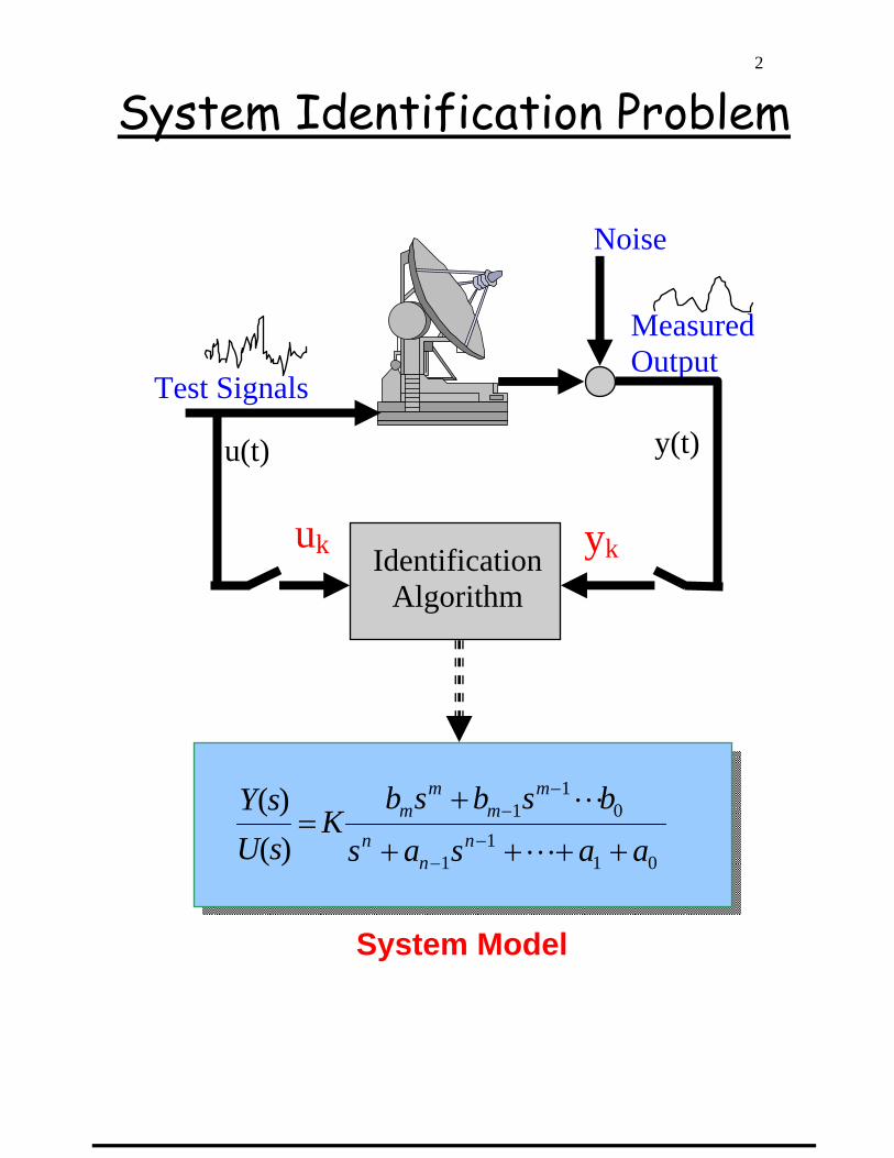
System Identification Problem

MeasuredOutput

011

1

01

1

)()(

aasasbsbsb

KsUsY

nn

n

mm

mm

++++

+=

−−

−−

L

L

IdentificationAlgorithm

Test Signals

Noise

uk yk

u(t) y(t)

System Model

3

Basic Elements of the System Identification Problem

• Model Structure

• Experiment Design

• Method for Selecting a Particular Model

• Validation of the Selected Model

Computer tools are required to support the various parts of the problem ! Example : Matlab/Simulink and the Identification Tool Box

4

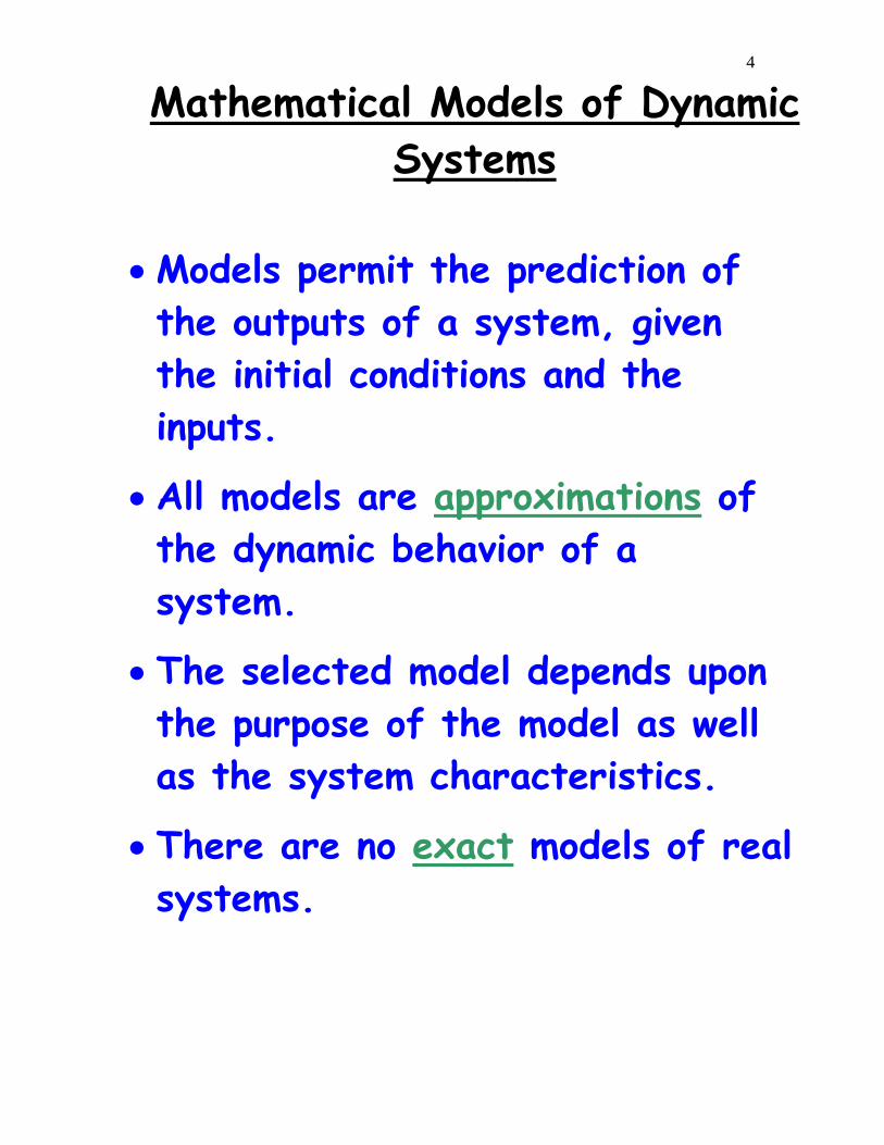
Mathematical Models of Dynamic Systems

• Models permit the prediction of the outputs of a system, given the initial conditions and the inputs.

• All models are approximations of the dynamic behavior of a system.

• The selected model depends upon the purpose of the model as well as the system characteristics.

• There are no exact models of real systems.

5

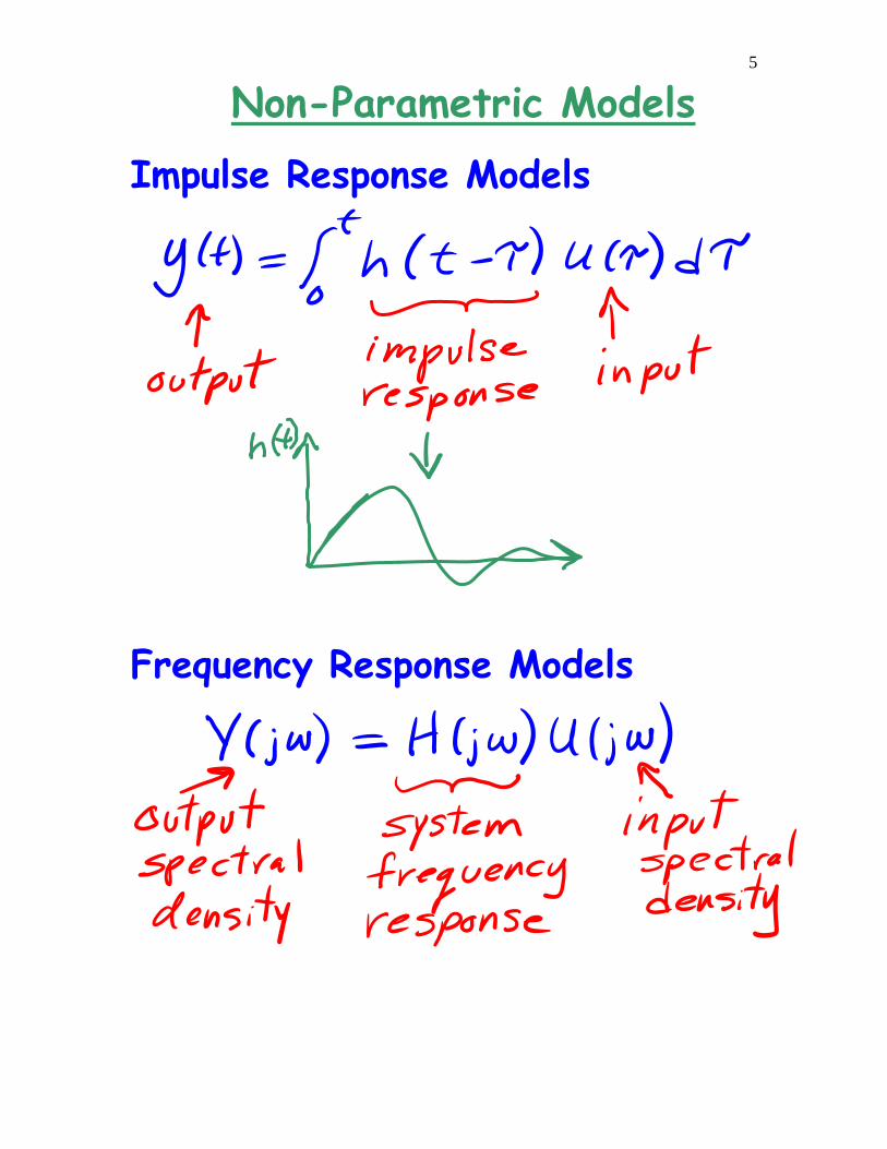
Non-Parametric Models Impulse Response Models

Frequency Response Models

6

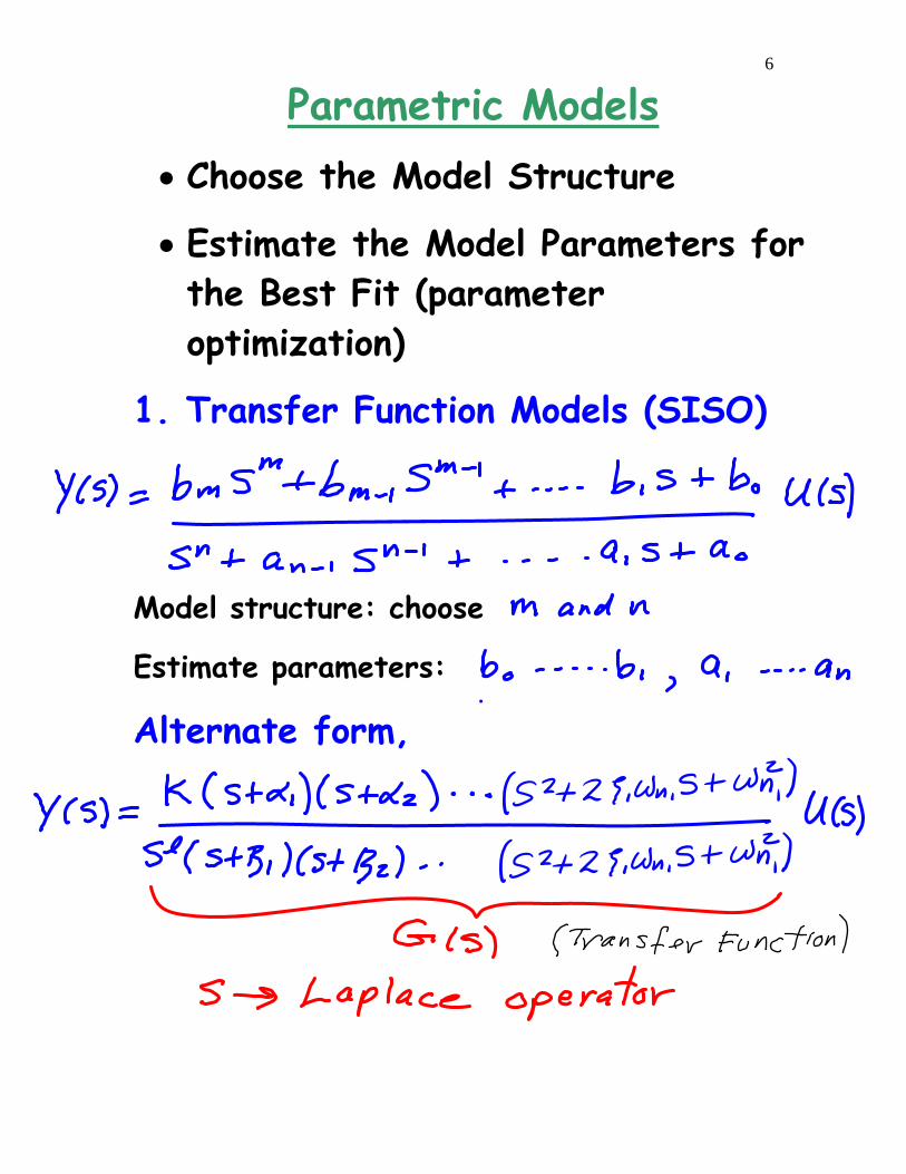
Parametric Models • Choose the Model Structure

• Estimate the Model Parameters for the Best Fit (parameter optimization)

1. Transfer Function Models (SISO)

Model structure: choose

Estimate parameters:

Alternate form,

7

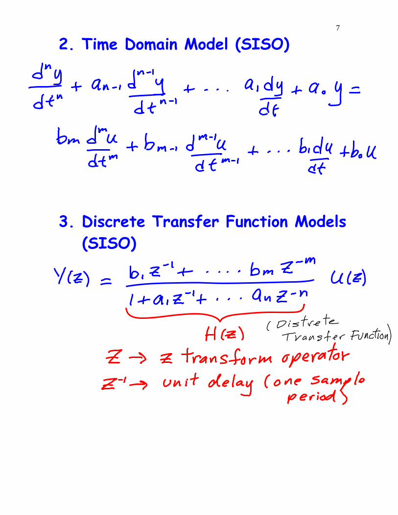
2. Time Domain Model (SISO)

3. Discrete Transfer Function Models (SISO)

8

4. Discrete Time Domain Models (SISO)

9

5. State Space Models (MIMO)

where

Structural parameters:

Model parameters (to be estimated):

Canonical forms: minimum parameter models

10

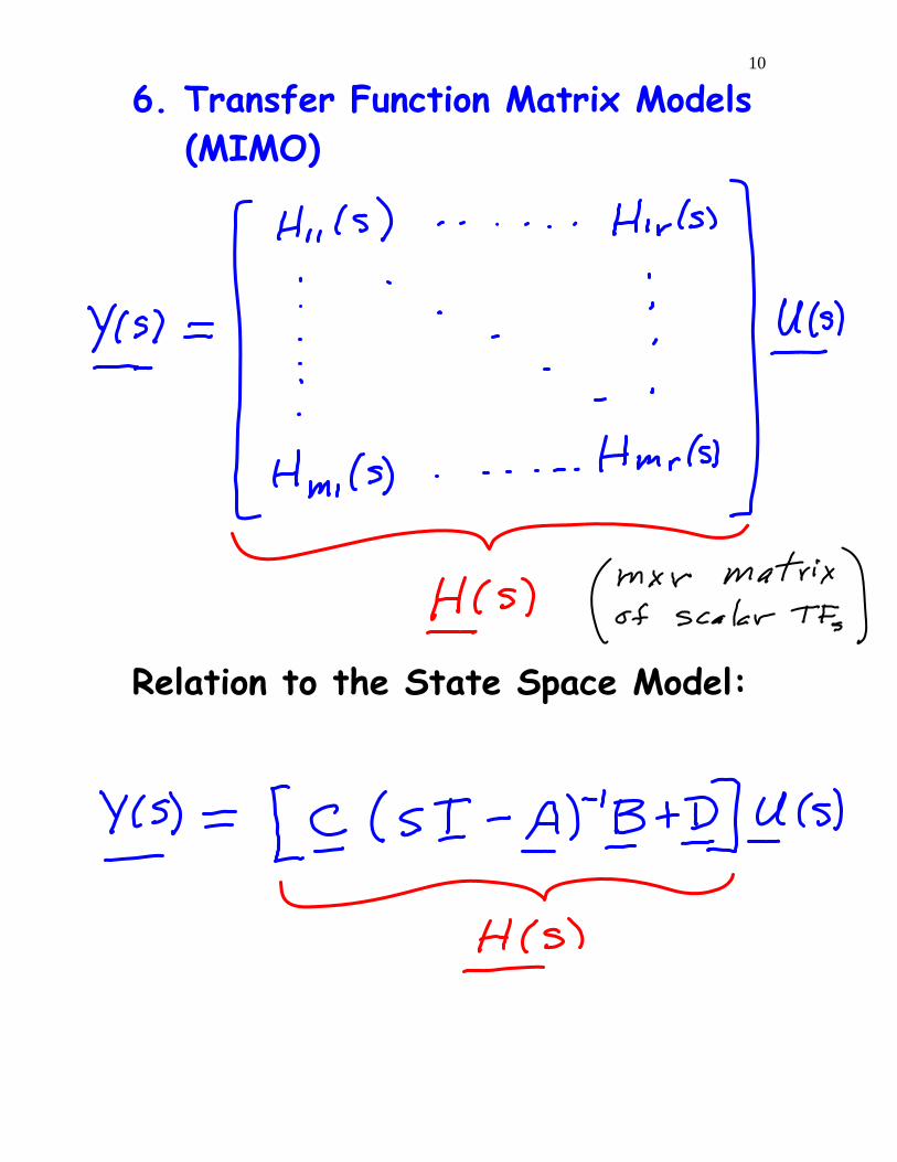
6. Transfer Function Matrix Models (MIMO)

Relation to the State Space Model:

11

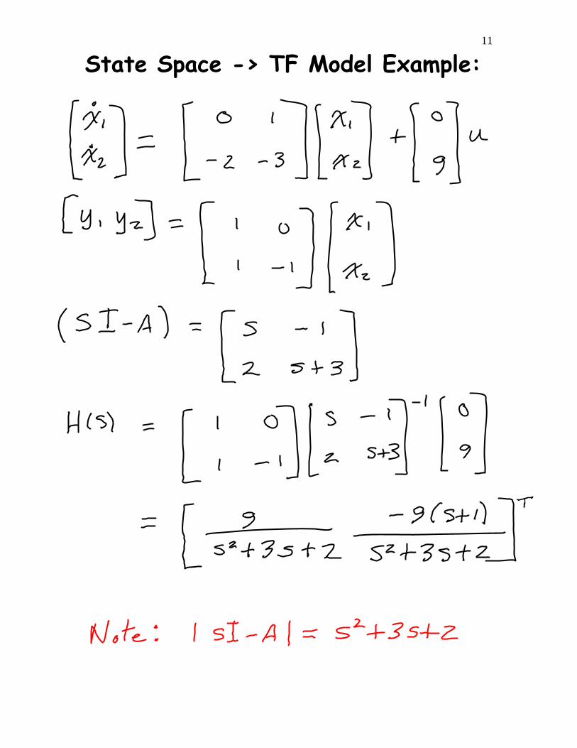
State Space -> TF Model Example:

12

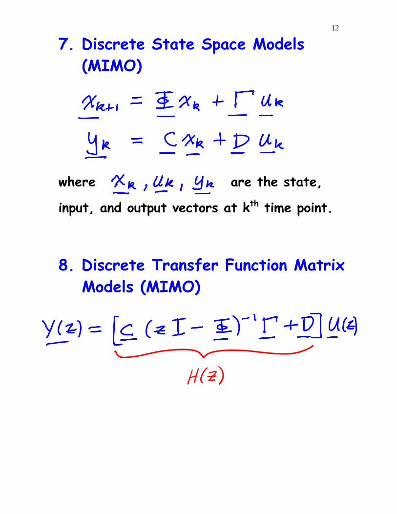
7. Discrete State Space Models (MIMO)

where are the state,

input, and output vectors at kth time point.

8. Discrete Transfer Function Matrix Models (MIMO)

13

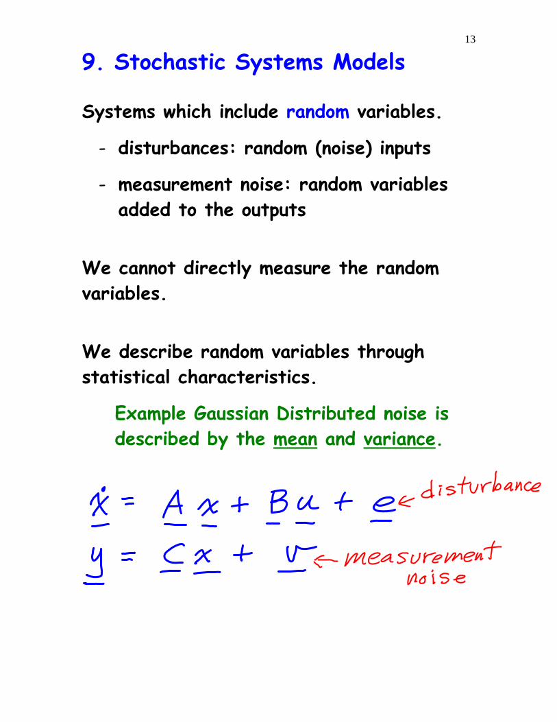
9. Stochastic Systems Models

Systems which include random variables.

- disturbances: random (noise) inputs

- measurement noise: random variables added to the outputs

We cannot directly measure the random variables.

We describe random variables through statistical characteristics.

Example Gaussian Distributed noise is described by the mean and variance.

14

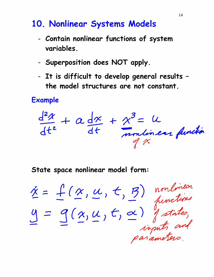
10. Nonlinear Systems Models - Contain nonlinear functions of system

variables.

- Superposition does NOT apply.

- It is difficult to develop general results – the model structures are not constant.

Example

State space nonlinear model form:

15

11. Discrete Nonlinear Systems Models

12. Time Varying Systems Models - System characteristics vary with time.

- Model parameters vary with time.

- Real-time tracking of parameters required.

16

Relationship Between Models - Some relationships are unique while others

are not.

- Some are exact while others are approximations.

- A summary is given on the following page.

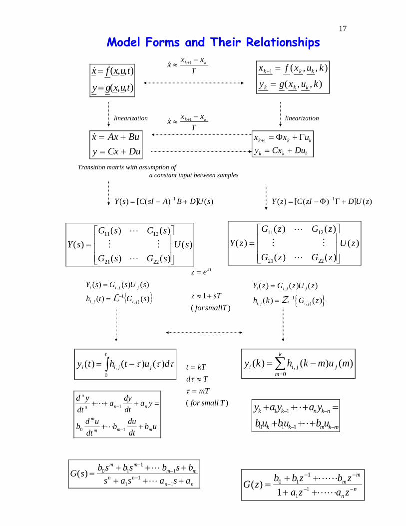
17

Model Forms and Their Relationships

linearization linearization

Transition matrix with assumption of a constant input between samples

&x x xT

k k≈−+1 x f x u k

y g x u kk k k

k k k

+ =

=1 ( , , )

( , , ) & ( , , )

( , , )

x f x u t

y g x u t

=

=

&x x xT

k k≈−+1

&x Ax Buy Cx Du= += +

x x uy Cx Du

k k k

k k k

+ = += +1 Φ Γ

Y s C sI A B D U s( ) [ ( ) ] ( )= − +−1 )(])([)( 1 zUDzICzY +ΓΦ−= −

Y sG s G s

G s G sU s( )

( ) ( )

( ) ( )( )=

⎡

⎣

⎢⎢⎢

⎤

⎦

⎥⎥⎥

11 12

21 22

L

M M

L

Y zG z G z

G z G zU z( )

( ) ( )

( ) ( )( )=

⎡

⎣

⎢⎢⎢

⎤

⎦

⎥⎥⎥

11 12

21 22

L

M M

L

)(1

TsmallforsTz

ez sT

+≈

=

{ })()(

)()()(

(,1

,

,

sGth

sUsGsY

jiji

jjii

−=

=

L { }

Y z G z U z

h k G zi i j j

i j i j

( ) ( ) ( )

( ) ( ),

, , (

=

= −Z 1

y t h t u di i j j

t

( ) ( ) ( ),= −∫ τ τ τ0

∑=

−=k

mjjii mumkhky

0, )()()( t kT

d TmT

for small T

=≈

=τ

τ( )

ubdtdub

dtudb

yadtdya

dtyd

mmm

m

nnn

n

++

=+++

−

−

10

1

L

L

mkmkk

nknkk

ubububyayay

−−

−−

+++=+++

L

L

110

11

G s b s b s b s bs a s a s a

m mm m

n nn n

( ) = + + ++ + +

−−

−−

0 11

1

11

1

L

L

nn

mm

zazazbzbbzG −−

−−

++++

=LL

LL1

1

110

1)(

18

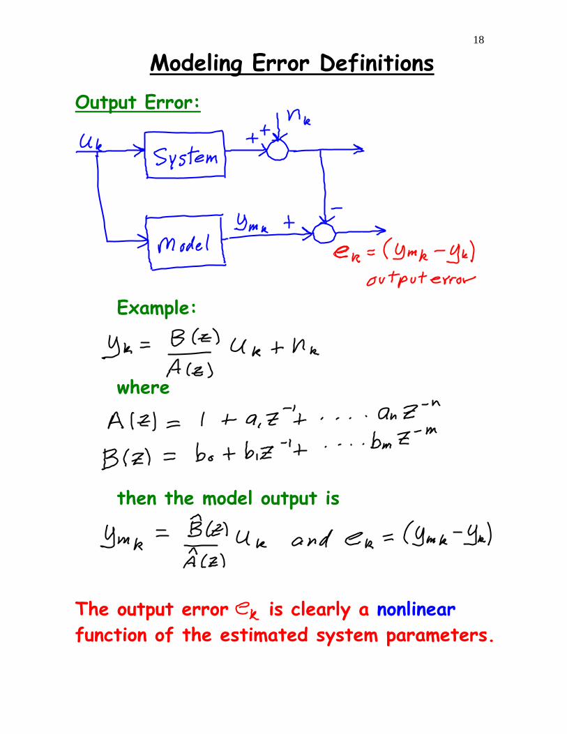
Modeling Error Definitions Output Error:

Example:

where

then the model output is

The output error is clearly a nonlinear function of the estimated system parameters.

19

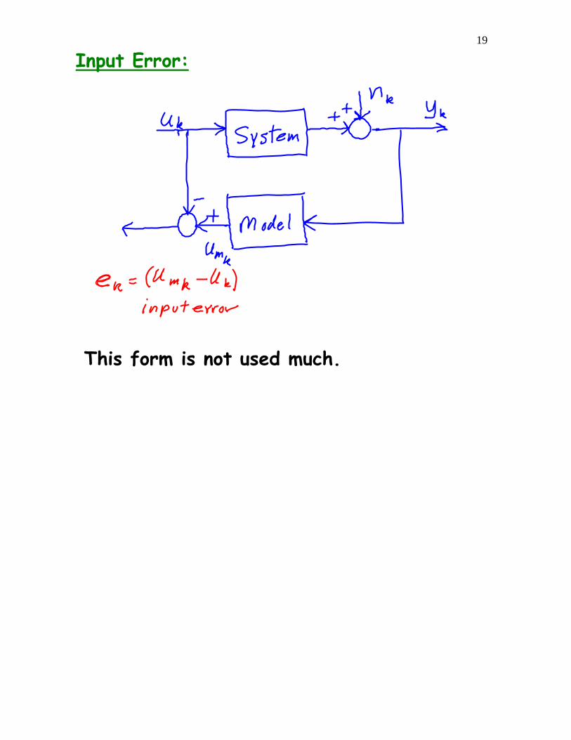
Input Error:

This form is not used much.

20

Generalized Error:

The generalized error is linear in the parameters, and therefore, linear parameter estimation may be used.

21

A Problem:

then

If is white noise, the generalized error will contain coloured raise, which causes significant problems in the parameter estimation process.

Consider Pre-whitening Filters:

Apply the same filter to the input and output sequences, . This should not cause any change in the input-output relationship over the admitted frequencies.

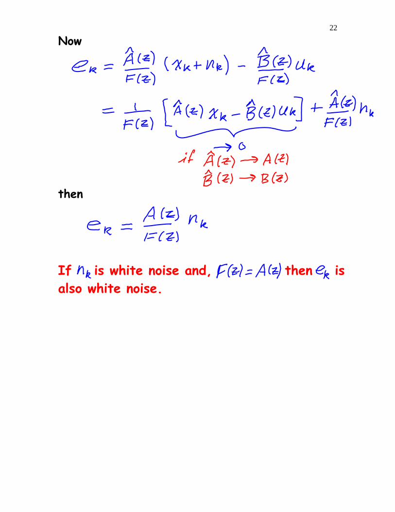
22

Now

then

If is white noise and, then is also white noise.

23

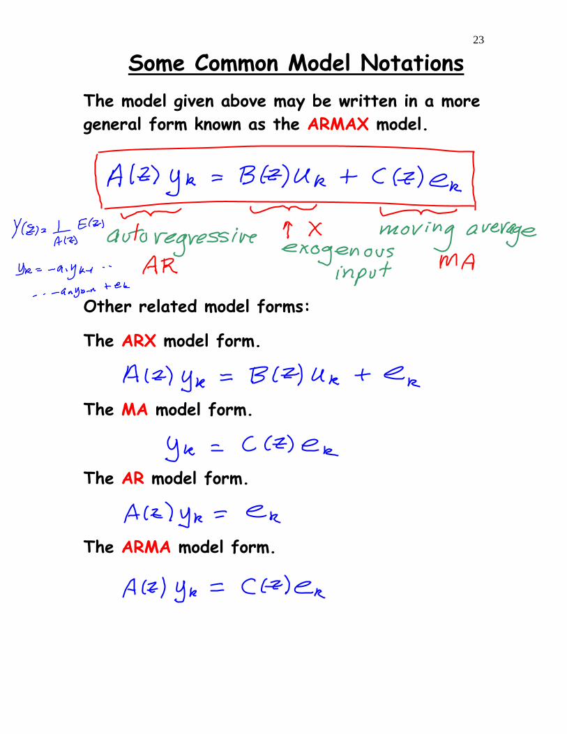
Some Common Model Notations The model given above may be written in a more general form known as the ARMAX model.

Other related model forms:

The ARX model form.

The MA model form.

The AR model form.

The ARMA model form.

24

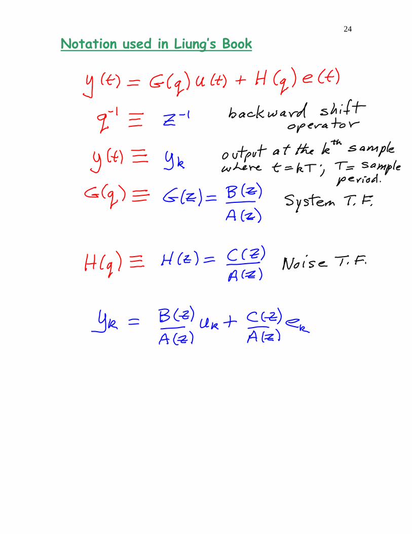
Notation used in Liung’s Book

25

Experiment Design

Choices:

a) Inputs

b) Data Collection

c) System Operating Condition

Inputs: size? periodic? noise?

- Periodic – sine wave, square wave, triangular wave, period, and offset.

- Non periodic – step, impulse (pulse), random.

- Random – white noise (approximation), pseudo random, PRBNS.

- Size – linear/nonlinear considerations, noise considerations, bias.

26

- Off-set – Signal perturbations about an operation condition.

Data Collection:

- Sample data – always

- Sample time (period) – dynamic considerations

- Length of data series – dynamic considerations

System Operating Condition:

- Nonlinear systems – operating point (steady state)

- Sequence of experiments at different operating points

- Normal plant inputs

- Superimpose test signals