SHYFEMFinite Element Model for Coastal Seas

User Manual

Georg UmgiesserISDGM-CNR, S. Polo 1364

30125 Venezia, Italy

Version 4.93

December 2, 2005

Contents

Disclaimer ii

1 Introduction 1

2 Equations and resolution techniques 22.1 Equations and Boundary Conditions . . . . . . . . . . . . . . . . . . . . . 22.2 The Model . . . . . . . . . . . . . . . . . . . . . . . . . . . . . . . . . . . 3

2.2.1 Discretization in Time - The Semi-Implicit Method . . . . . . . . . 32.2.2 Discretization in Space - The Finite Element Method . . . . . . . . 42.2.3 Mass Conservation . . . . . . . . . . . . . . . . . . . . . . . . . . 72.2.4 Inter-tidal Flats . . . . . . . . . . . . . . . . . . . . . . . . . . . . 7

3 Pre-Processing 83.1 The pre-processing routine vp . . . . . . . . . . . . . . . . . . . . . . . . 83.2 Optimization of the bandwidth . . . . . . . . . . . . . . . . . . . . . . . . 83.3 Internal and external node numbering . . . . . . . . . . . . . . . . . . . . 9

4 The Model 104.1 The Parameter Input File . . . . . . . . . . . . . . . . . . . . . . . . . . . 10

4.1.1 The General Structure of the Parameter Input File . . . . . . . . . . 104.1.2 The Single Sections of the Parameter Input File . . . . . . . . . . . 11

5 Post-Processing 225.1 Plotting of maps with plotmap . . . . . . . . . . . . . . . . . . . . . . . . 22

5.1.1 The parameter input file for plotmap . . . . . . . . . . . . . . . . 22

6 The Water Quality Module 266.1 General Description . . . . . . . . . . . . . . . . . . . . . . . . . . . . . . 266.2 The coupling . . . . . . . . . . . . . . . . . . . . . . . . . . . . . . . . . 276.3 Light limitation . . . . . . . . . . . . . . . . . . . . . . . . . . . . . . . . 33

6.3.1 Light attenuation formula by Steele and Di Toro . . . . . . . . . . 336.3.2 Light attenuation formula by Smith . . . . . . . . . . . . . . . . . 33

6.4 Initialization . . . . . . . . . . . . . . . . . . . . . . . . . . . . . . . . . . 346.5 Post processing . . . . . . . . . . . . . . . . . . . . . . . . . . . . . . . . 346.6 The Sediment Module . . . . . . . . . . . . . . . . . . . . . . . . . . . . . 35

6.6.1 Parameters for the Water Quality Module . . . . . . . . . . . . . . 37

Bibliography 38

i

Disclaimer

Copyright (c) 1992-1998 by Georg UmgiesserPermission to use, copy, modify, and distribute this software and its docu-

mentation for any purpose and without fee is hereby granted, provided that theabove copyright notice appear in all copies and that both that copyright noticeand this permission notice appear in supporting documentation.

This file is provided AS IS with no warranties of any kind. The author shallhave no liability with respect to the infringement of copyrights, trade secretsor any patents by this file or any part thereof. In no event will the author beliable for any lost revenue or profits or other special, indirect and consequentialdamages.

Comments and additions should be sent to the author:

Georg UmgiesserISDGM/CNRS. Polo 136430125 VeneziaItaly

Tel. : ++39-41-5216875Fax : ++39-41-2602340E-Mail : georg@lagoon.isdgm.ve.cnr.it

ii

Chapter 1

Introduction

The finite element program SHYFEM is a program package that can be used to resolve the hy-drodynamic equations in lagoons, coastal seas, estuaries and lakes. The program uses finiteelements for the resolution of the hydrodynamic equations. These finite elements, togetherwith an effective semi-implicit time resolution algorithm, makes this program especiallysuitable for application to a complicated geometry and bathymetry.This version of the program SHYFEM resolves the depth integrated shallow water equations.It is therefore recommended for the application of very shallow basins or well mixed estu-aries. Storm surge phenomena can be investigated also. This two-dimensional version ofthe program is not suited for the application to baroclinic driven flows or large scale flowswhere the the Coriolis acceleration is important.Finite elements are superior to finite differences when dealing with complex bathymetricsituations and geometries. Finite differences are limited to a regular outlay of their grids.This will be a problem if only parts of a basin need high resolution. The finite elementmethod has an advantage in this case allowing more flexibility with its subdivision of thesystem in triangles varying in form and size.This model is especially adapted to run in very shallow basins. It is possible to simulateshallow water flats, i.e., tidal marshes that in a tidal cycle may be covered with water duringhigh tide and then fall dry during ebb tide. This phenomenon is handled by the model in amass conserving way.Finite element methods have been introduced into hydrodynamics since 1973 and havebeen extensively applied to shallow water equations by numerous authors [3, 9, 5, 4, 6].The model presented here [10, 11] uses the mathematical formulation of the semi-implicitalgorithm that decouples the solution of the water levels and velocity components fromeach other leading to smaller systems to solve. Models of this type have been presentedfrom 1971 on by many authors [7, 2, 1].

1

Chapter 2

Equations and resolutiontechniques

2.1 Equations and Boundary ConditionsThe equations used in the model are the well known vertically integrated shallow waterequations in their formulation with water levels and transports.

∂U∂t

+gH∂ζ

∂x+RU +X = 0 (2.1)

∂V∂t

+gH∂ζ

∂y+RV +Y = 0 (2.2)

∂ζ

∂t+

∂U∂x

+∂V∂y

= 0 (2.3)

where ζ is the water level, u,v the velocities in x and y direction, U,V the vertical integratedvelocities (total or barotropic transports)

U =Z

ζ

−hu dz V =

Zζ

−hv dz

g the gravitational acceleration, H = h + ζ the total water depth, h the undisturbed waterdepth, t the time and R the friction coefficient. The terms X ,Y contain all other terms thatmay be added to the equations like the wind stress or the nonlinear terms and that need notbe treated implicitly in the time discretization. following treatment.The friction coefficient has been expressed as

R =g√

u2 + v2

C2H(2.4)

with C the Chezy coefficient. The Chezy term is itself not retained constant but varies withthe water depth as

C = ksH1/6 (2.5)

where ks is the Strickler coefficient.In this version of the model the Coriolis term, the turbulent friction term and the nonlinearadvective terms have not been implemented.At open boundaries the water levels are prescribed. At closed boundaries the normal ve-locity component is set to zero whereas the tangential velocity is a free parameter. Thiscorresponds to a full slip condition.

2

2.2 The ModelThe model uses the semi-implicit time discretization to accomplish the time integration.In the space the finite element method has been used, not in its standard formulation, butusing staggered finite elements. In the following a description of the method is given.

2.2.1 Discretization in Time - The Semi-Implicit MethodLooking for an efficient time integration method a semi-implicit scheme has been chosen.The semi-implicit scheme combines the advantages of the explicit and the implicit scheme.It is unconditionally stable for any time step ∆t chosen and allows the two momentumequations to be solved explicitly without solving a linear system.The only equation that has to be solved implicitly is the continuity equation. Comparedto a fully implicit solution of the shallow water equations the dimensions of the matrix arereduced to one third. Since the solution of a linear system is roughly proportional to thecube of the dimension of the system the saving in computing time is approximately a factorof 30.It has to be pointed out that it is important not to be limited with the time step by the CFLcriterion for the speed of the external gravity waves

∆t <∆x√gH

where ∆x is the minimum distance between the nodes in an element. With the discretizationdescribed below in most parts of the lagoon we have ∆x ≈ 500m and H ≈ 1m, so ∆t ≈ 200sec. But the limitation of the time step is determined by the worst case. For example, for∆x = 100 m and H = 40 m the time step criterion would be ∆t < 5 sec, a prohibitive smallvalue.The equations (1)-(3) are discretized as follows

ζn+1−ζn

∆t+ 1

2∂(Un+1 +Un)

∂x+ 1

2∂(V n+1 +V n)

∂y= 0 (2.6)

Un+1−Un

∆t+gH 1

2∂(ζn+1 +ζn)

∂x+RUn+1 +X = 0 (2.7)

V n+1−V n

∆t+gH 1

2∂(ζn+1 +ζn)

∂y+RV n+1 +Y = 0 (2.8)

With this time discretization the friction term has been formulated fully implicit, X ,Y fullyexplicit and all the other terms have been centered in time. The reason for the implicittreatment of the friction term is to avoid a sign inversion in the term when the frictionparameter gets too high. An example of this behavior is given in Backhaus [1].If the two momentum equations are solved for the unknowns Un+1 and V n+1 we have

Un+1 =1

1+∆tR

(Un−∆tgH 1

2∂(ζn+1 +ζn)

∂x−∆tX

)(2.9)

V n+1 =1

1+∆tR

(V n−∆tgH 1

2∂(ζn+1 +ζn)

∂y−∆tY

)(2.10)

If ζn+1 were known, the solution for Un+1 and V n+1 could directly be given. To find ζn+1

we insert (2.9) and (2.10) in (2.6). After some transformations (2.6) reads

ζn+1 − (∆t/2)2 g1+∆tR

(∂

∂x(H ∂ζn+1

∂x)+

∂

∂y(H ∂ζn+1

∂y))

3

= ζn +(∆t/2)2 g1+∆tR

(∂

∂x(H ∂ζn

∂x)+

∂

∂y(H ∂ζn

∂y))

(2.11)

− (∆t/2)(

2+∆tR1+∆tR

)(∂Un

∂x+

∂V n

∂y

)+

∆t2

2(1+∆tR)

(∂X∂x

+∂Y∂y

)The terms on the left hand side contain the unknown ζn+1, the right hand contains onlyknown values of the old time level. If the spatial derivatives are now expressed by the finiteelement method a linear system with the unknown ζn+1 is obtained and can be solved bystandard methods. Once the solution for ζn+1 is obtained it can be substituted into (2.9)and (2.10) and these two equations can be solved explicitly. In this way all unknowns ofthe new time step have been found.Note that the variable H also contains the water level through H = h+ζ. In order to avoidthe equations to become nonlinear ζ is evaluated at the old time level so H = h+ζn and His a known quantity.

2.2.2 Discretization in Space - The Finite Element MethodWhile the time discretization has been explained above, the discretization in space has stillto be carried out. This is done using staggered finite elements. With the semi-implicitmethod described above it is shown below that using linear triangular elements for allunknowns will not be mass conserving. Furthermore the resulting model will have propa-gation properties that introduce high numeric damping in the solution of the equations.For these reasons a quite new approach has been adopted here. The water levels and thevelocities (transports) are described by using form functions of different order, being thestandard linear form functions for the water levels but stepwise constant form functionsfor the transports. This will result in a grid that resembles more a staggered grid in finitedifference discretizations.

Formalism

Let u be an approximate solution of a linear differential equation L. We expand u with thehelp of basis functions φm as

u = φmum m = 1,K (2.12)

where um is the coefficient of the function φm and K is the order of the approximation. Incase of linear finite elements it will just be the number of nodes of the grid used to discretizethe domain.To find the values um we try to minimize the residual that arises when u is introduced into Lmultiplying the equation L by some weighting functions Ψn and integrating over the wholedomain leading toZ

Ω

ψnL(u)dΩ =Z

Ω

ψnL(φmum)dΩ = um

ZΩ

ψnL(φm)dΩ (2.13)

If the integral is identified with the elements of a matrix anm we can write (2.13) also as alinear system

anmum = 0 n = 1,K m = 1,K (2.14)

Once the basis and weighting functions have been specified the system may be set up and(2.14) may be solved for the unknowns um.

4

Figure 2.1: a) form functions in domain b) domain of influence of node i

JJJJ

PPP

AAAA

XXXX C

CCC

PPP

CCCC

H

HH

H

QQQLLLLLL

@@@

SSSS

aaaa

a

AAAA

XXXX

@@

@

AA

EEEEEEE

SS

SS

n

iφi

ψn

tt

t t

ff

fff

f

JJJJ

PPP

AAAA

XXXX C

CCC

PPP

CCCC

HH

HH

QQQLLLLLL

@@@

SSSS

aaaa

a

AAAA

XXXX

ij tt

t t tt

f ff

fff

f

Staggered Finite Elements

For decades finite elements have been used in fluid mechanics in a standardized manner.The form functions φm were chosen as continuous piecewise linear functions allowing asubdivision of the whole area of interest into small triangular elements specifying the coef-ficients um at the vertices (called nodes) of the triangles. The functions φm are 1 at node mand 0 at all other nodes and thus different from 0 only in the triangles containing the nodem. An example is given in the upper left part of Fig. 1a where the form function for node iis shown. The full circle indicates the node where the function φi take the value 1 and thehollow circles where they are 0.The contributions anm to the system matrix are therefore different from 0 only in elementscontaining node m and the evaluation of the matrix elements can be performed on an ele-ment basis where all coefficients and unknowns are linear functions of x and y.This approach is straightforward but not very satisfying with the semi-implicit time step-ping scheme for reasons explained below. Therefore an other way has been followed inthe present formulation. The fluid domain is still divided in triangles and the water levelsare still defined at the nodes of the grid and represented by piecewise linear interpolatingfunctions in the internal of each element, i.e.

ζ = ζmφm m = 1,K

However, the transports are now expanded, over each triangle, with piecewise constant (noncontinuous) form functions ψn over the whole domain. We therefore write

U = Unψn n = 1,J

where n is now running over all triangles and J is the total number of triangles. An exampleof ψn is given in the lower right part of Fig. 1a. Note that the form function is constant 1over the whole element, but outside the element identically 0. Thus it is discontinuous atthe element borders.Since we may identify the center of gravity of the triangle with the point where the trans-ports Un are defined (contrary to the water levels ζm which are defined on the vertices ofthe triangles), the resulting grid may be seen as a staggered grid where the unknowns aredefined on different locations. This kind of grid is usually used with the finite differencemethod. With the form functions used here the grid of the finite element model resemblesvery much an Arakawa B-grid that defines the water levels on the center and the velocitieson the four vertices of a square.Staggered finite elements have been first introduced into fluid mechanics by Schoenstadt[8]. He showed that the un-staggered finite element formulation of the shallow water equa-tions has very poor geostrophic adjustment properties. Williams [12, 13] proposed a similar

5

algorithm, the one actually used in this paper, introducing constant form functions for thevelocities. He showed the excellent propagation and geostrophic adjustment properties ofthis scheme.

The Practical Realization

The integration of the partial differential equation is now performed by using the subdivi-sion of the domain in elements (triangles). The water levels ζ are expanded in piecewiselinear functions φm, m = 1,K and the transports are expanded in piecewise constant func-tions ψn, n = 1,J where K and J are the total number of nodes and elements respectively.As weighting functions we use ψn for the momentum equations and φm for the continuityequation. In this way there will be K equations for the unknowns ζ (one for each node) andJ equations for the transports (one for each element).In all cases the consistent mass matrix has been substituted with the their lumped equiva-lent. This was mainly done to avoid solving a linear system in the case of the momentumequations. But it was of use also in the solution of the continuity equation because theamount of mass relative to one node does not depend on the surrounding nodes. This wasimportant especially for the flood and dry mechanism in order to conserve mass.

Finite Element Equations

If equations (2.9,2.10,2.11) are multiplied with their weighting functions and integratedover an element we can write down the finite element equations. But the solution of thewater levels does actually not use the continuity equation in the form (2.11), but a slightlydifferent formulation. Starting from equation (2.6), multiplied by the weighting functionΦM and integrated over one element yieldsZ

Ω

ΦN(ζn+1−ζn)dΩ +(∆t2 )

ZΩ

(ΦN

∂(Un+1 +Un)∂x

+ΦN∂(V n+1 +V n)

∂y

)dΩ = 0

If we integrate by parts the last two integrals we obtainZΩ

ΦN(ζn+1−ζn)dΩ − (∆t2 )

ZΩ

(∂ΦN

∂x(Un+1 +Un)+

∂ΦN

∂y(V n+1 +V n)

)dΩ = 0

plus two line integrals, not shown, over the boundary of each element that specify thenormal flux over the three element sides. In the interior of the domain, once all contribu-tions of all elements have been summed, these terms cancel at every node, leaving onlythe contribution of the line integral on the boundary of the domain. There, however, theboundary condition to impose is exactly no normal flux over material boundaries. Thus,the contribution of these line integrals is zero.If now the expressions for Un+1,V n+1 are introduced, we obtain a system with again onlythe water levels as unknownsZ

Ω

ΦNζn+1 dΩ + (∆t/2)2αg

ZΩ

H(∂ΦN

∂x∂ζn+1

∂x+

∂ΦN

∂y∂ζn+1

∂y)dΩ

=Z

Ω

ΦNζn dΩ +(∆t/2)2αg

ZΩ

H(∂ΦN

∂x∂ζn

∂x+

∂ΦN

∂y∂ζn

∂y)dΩ

+ (∆t/2)(1+α)Z

Ω

(∂ΦN

∂xUn +

∂ΦN

∂yV n)dΩ (2.15)

− (∆t2/2)αZ

Ω

(∂ΦN

∂xX +

∂ΦN

∂yY )dΩ

Here we have introduced the symbol α as a shortcut for

α =1

1+∆tR

6

The variables and unknowns may now be expanded with their basis functions and the com-plete system may be set up.

2.2.3 Mass ConservationIt should be pointed out that only through the use of this staggered grid the semi-implicittime discretization may be implemented in a feasible manner. If the Galerkin method isapplied in a naive way to the resulting equation (2.11) (introducing the linear form func-tions for transports and water levels and setting up the system matrix), the model is notmass conserving. This may be seen in the following way (see Fig. 1b for reference). In thecomputation of the water level at node i, only ζ and transport values belonging to trianglesthat contain node i enter the computation (full circles in Fig. 1b). But when, in a secondstep, the barotropic transports of node j are computed, water levels of nodes that lie furtherapart from the original node i are used (hollow circles in Fig. 1b). These water levels havenot been included in the computation of ζi, the water level at node i. So the computed trans-ports are actually different from the transports inserted formally in the continuity equation.The continuity equation is therefore not satisfied.These contributions of nodes lying further apart could in principle be accounted for. In thiscase not only the triangles Ωi around node i but also all the triangles that have nodes incommon with the triangles Ωi would give contributions to node i, namely all nodes andelements shown in Fig. 1b. The result would be an increase of the bandwidth of the matrixfor the ζ computation disadvantageous in terms of memory and time requirements.Using instead the approach of the staggered finite elements, actually only the water levelsof elements around node i are needed for the computation of the transports in the trianglesΩi. In this case the model satisfies the continuity equation and is perfectly mass conserving.

2.2.4 Inter-tidal FlatsPart of a basin may consist of areas that are flooded during high tides and emerge as islandsat ebb tide. These inter-tidal flats are quite difficult to handle numerically because theelements that represent these areas are neither islands nor water elements. The boundaryline defining their contours is wandering during the evolution of time and a mathematicalmodel must reproduce this features.For reasons of computer time savings a simplified algorithm has been chosen to representthe inter-tidal flats. When the water level in at least one of the three nodes of an elementfalls below a minimum value (5 cm) the element is considered an island and is taken outof the system. It will be reintroduced only when in all three nodes the water level is againhigher then the minimum value. Because in dry nodes no water level is computed anymore,an estimate of the water level has to be given with some sort of extrapolation mechanismusing the water nodes nearby.This algorithm has the advantage that it is very easy to implement and very fast. Thedynamical features close to the inter-tidal flats are of course not well reproduced but thebehavior of the method for the rest of the lagoon gave satisfactory results.In any case, since the method stores the water levels of the last time step, before the ele-ment is switched off, introducing the element in a later moment with the same water levelsconserves the mass balance. This method showed a much better performance than the onewhere the new elements were introduced with the water levels taken from the extrapolationof the surrounding nodes.

7

Chapter 3

Pre-Processing

The pre-processing routine vp is used to generate an optimized version of the file that de-scribes the basin where the main program is to be run. In the following a short introductionin using this program is given.

3.1 The pre-processing routine vpThe main routine hp reads the basin file generated by the pre-processing routine vp and usesit as the description of the domain where the hydrodynamic equations have to be solved.The program vp is started by typing vp on the command line. From this point on theprogram is interactive, asking you about the basin file name and other options. Pleasefollow the online instructions.The routine vp reads a file of type GRD. This type of file can be generated and manipulatedby the program grid which is not described here. In short, the file GRD consists of nodesand elements that describe the geometrical layout of the basin. Moreover, the elementshave a type and a depth.The depth is needed by the main program hp to run the model. The type of the element isused by hp to determine the friction parameter on the bottom, since this parameter may beassigned differently, depending on the various situations of the bottom roughness.This file GRD is read by vp and transformed into an unformatted file BAS. It is this file thatis then read by the main routine hp. Therefore, if the name of the basin is lagoon, then thefile GRD is called lagoon.grd and the output of the pre-processing routine vp is calledlagoon.bas.The program vp normally uses the depths assigned to the elements in the file GRD todetermine the depth of the finite elements to use in the program hp. In the case that thesedepth values are not complete, and that all nodes have depths assigned in the GRD file, thenodal values of the depths are used and interpolated onto the elements. However, if alsothese nodal depth values are incomplete or are missing altogether, the program terminateswith an error.

3.2 Optimization of the bandwidthThe main task of routine vp is the optimization of the internal numbering of the nodes andelements. Re-numbering the elements is just a mere convenience. When assembling thesystem matrix the contribution of one element after the other has to be added to the systemmatrix. If the elements are numbered in terms of lowest node numbers, then the accessof the nodal pointers is more regular in computer memory and paging is more likely to beinhibited.

8

However, re-numbering the nodes is absolutely necessary. The system matrix to be solvedis of band-matrix type. I.e., non-zero entries are all concentrated along the main diagonalin a more or less narrow band. The larger this band is, the larger the amount of cpu timespent to solve the system. The time to solve a band matrix is of order n ·m2, where n is thesize of the matrix and m is the bandwidth. Note that m is normally much smaller than n.If the nodes are left with the original numbering, it is very likely that the bandwidth isvery high, unless the nodes in the file GRD are by chance already optimized. Since thebandwidth m is entering the above formula quadratically, the amount of time spent solvingthe matrix will be prohibitive. E.g., halving the bandwidth will speed up computations bya factor of 4.The bandwidth is equal to the maximum difference of node numbers in one element. It istherefore important to re-number the nodes in order to minimize this number. However,there exist only heuristic algorithms for the minimization of this number.The two main algorithms used in the routine vp are the Cuthill McGee algorithm and thealgorithm of Rosen. The first one, starting from one node, tries to number all neighbors ina greedy way, optimizing only this step. From the points numbered in this step, the nextneighbors are numbered.This procedure is tried from more than one node, possibly from all boundary nodes. Thenumbering resulting from this algorithm is normally very good and needs only slight en-hancements to be optimum.Once all nodes are numbered, the Rosen algorithm tries to exchange these node numbers,where the highest difference can be found. This normally gives only a slight improvementof the bandwidth. It has been seen, however, that, if the node numbers coming out from theCuthill McGee algorithm are reversed, before feeding them into the Rosen algorithm, theresults tend to be slightly better. This step is also performed by the program.All these steps are performed by the program without intervention by the operator, if theautomatic optimization of bandwidth is chosen in the program vp. The choices are to notperform the bandwidth optimization at all (GRD file has already optimized node number-ing), perform it automatically or perform it manually. It is suggested to always performautomatic optimization of the bandwidth. This choice will lead to a nearly optimum num-bering of the nodes and will be by all means good results.If, however, you decide to do a manual optimization, please follow the online instructionsin the program.

3.3 Internal and external node numberingAs explained above, the elements and nodes of the basin are re-numbered in order to opti-mize the bandwidth of the system matrix and so the execution speed of the program.However, this re-numbering of the node and elements is transparent to the user. The pro-gram keeps pointers from the original numbering (external numbers) to the optimized num-bering (internal numbers). The user has to deal only with external numbers, even if theprogram uses internally the other number system.Moreover, the internal numbers are generated consecutively. Therefore, if there are a totalof 4000 nodes in the system, the internal nodes run from 1 to 4000. The external nodenumbers, on the other side, can be anything the user likes. They just must be unique. Thisallows for insertion and deletion of nodes without having to re-number over and over againthe basin.The nodes that have to be specified in the input parameter file use again external numbers.In this way, changing the structure of the basin does not at all change the node and elementnumbers in the input parameter file. Except in the case, where modifications actually touchnodes and elements that are specified in the parameter file.

9

Chapter 4

The Model

In the following an overview is given on running the model SHYFEM. The model needs aparameter input file that is read on standard input. Moreover, it needs some external filesthat are specified in this parameter input file. The model produces several external fileswith the results of the simulation. Again, the name of this files can be influenced by theparameter input file

4.1 The Parameter Input FileThe model reads one input file that determines the behavior of the simulation. All possibleparameters can and must be set in this file. If other data files are to be read, here is the placewhere to specify them.The model reads this parameter file from standard input. Thus, if the model binary is calledhp and the parameter file param.str, then the following line starts the simulation

hp < param.str

and runs the model.

4.1.1 The General Structure of the Parameter Input FileThe input parameter file is the file that guides program performance. It contains all nec-essary information for the main routine to execute the model. Nearly all parameters thatcan be given have a default value which is used when the parameter is not listed in the file.Only some time parameters are compulsory and must be present in the file.The format of the file looks very like a namelist format, but is not dependent on the compilerused. Values of parameters are given in the form : name = value or name = ’text’. Ifname is an array the following format is used :

name = value1 , value2, ... valueN

The list can continue on the following lines. Blanks before and after the equal sign areignored. More then one parameter can be present on one line. As separator blank, tab andcomma can be used.Parameters, arrays and data must be given in between certain sections. A section startswith the character $ followed by a keyword and ends with $end. The $keyword and $endmust not contain any blank characters and must be the first non blank characters in the line.Other characters following the keyword on the same line separated by a valid separator areignored.Several sections of data may be present in the input parameter file. Further ahead all sec-tions are presented and the possible parameters that can be specified are explained. The

10

sequence in which the sections appear is of no importance. However, the first section mustalways be section \$title, the section that determines the name of simulation and thebasin file to use and gives a one line description of the simulation.Lines outside of the sections are ignored. This gives the possibility to comment the param-eter input file.Figure 4.1 shows an example of a typical input parameter file and the use of the sectionsand definition of parameters.

4.1.2 The Single Sections of the Parameter Input FileSection $title

This section must be always the first section in the parameter input file. It contains onlythree lines. An example is given in figure 4.2.The first line of this section is a free one line description of the simulation that is to be car-ried out. The next line contains the name of the simulation (in this case name_of_simulation).All created files will use this name in the main part of the file name with different exten-sions. Therefore the hydrodynamic output file (extension out) will be named name_of_simulation.out.The last line gives the name of the basin file to be used. This is the pre-processed file of thebasin with extension bas. In our example the basin file name_of_basin.bas is used.The directory where this files are read from or written to depends on the settings in section$name. Using the default the program will read from and write to the current directory.

Section $para

This section defines the general behavior of the simulation, gives various constants of pa-rameters and determines what output files are written. In the following the meaning of allpossible parameters is given.Note that the only compulsory parameters in this section are the ones that chose the durationof the simulation and the integration time step. All other parameters are optional.

Compulsory time parameters This parameters are compulsory parameters that definethe period of the simulation. They must be present in all cases.

itanf Start of simulation. (Default 0)

itend End of simulation.

idt Time step of integration.

Output parameters The following parameters deal with the output frequency and starttime to external files. The content of the various output files should be looked up in theappropriate section.The default for the time step of output of the files is 0 which means that no output file iswritten. If the time step of the output files is equal to the time step of the simulation then atevery time step the output file is written. The default start time of the output is 0.

idtoutitmout

Time step and start time for writing to file OUT, the file containing thegeneral hydrodynamic results.

idtextitmext

Time step and start time for writing to file EXT, the file containing hy-drodynamic data of extra points. The extra points for which the data iswritten to this file are given in section extra of the parameter file.

idtrstitmrst

Time step and start time for writing the restart

11

$titlebenchmark test for test lagoonbenchvenlag

$end

$paraitanf = 0 itend = 86400 idt = 300ireib = 2 ilin = 0href = 0.23 iczv = 1

$end

$bound1kbound = 73 74 76ampli = 0.50 period = 43200. phase = 10800. zref = 0.

$end

$bound2kbound = 353,350, 349iqual = 1

$end

$bound3kbound = 1374 1154 1160 1161iqual = 1

$end

$namewind=’win18sep.win’

$end

-------------- MAREOGRAFI PER TARATURA--------------13,133,99,259,328,772,419,1141,1195,1070,1064,942,468,1154-----------------------------------------------------

$extra ------- MAREOGRAFI + SEZIONI PER TARATURA----------13,133,99,259,328,772,419,1141,1195,1070,1064,942,468,115473,74,76,353,350,349,1374,1154,1160,1161,408,409,786,795$end

$area ------- old chezy values ----------0 33.1 25. 27. 74 752 21. 23. 350 3463 20. 25. 1154 11534 27.5 27.6 27.

$end

Figure 4.1: Example of a parameter input file

12

$titlefree one line description of simulationname_of_simulationname_of_basin

$end

Figure 4.2: Example of section $title

file (extension RST). No restart file is written with idtrst equal to 0. itrst Time to usefor the restart. If a restart is performed, then the file name containing the restart data has tobe specified in restrt and the time record corresponding to itrst is used in this file.

idtresitmres

Time step and start time for writing to file RES, the file containing resid-ual hydrodynamic data.

idtrmsitmrms

Time step and start time for writing to file RMS, the file containinghydrodynamic data of root mean square velocities.

idtflxitmflx

Time step and start time for writing to file FLX, the file containing dis-charge data through defined sections. The transects for which the dis-charges are computed are given in section flux of the parameter file.

Model parameters The next parameters define the inclusion or exclusion of certain termsof the primitive equations.

ilin Linearization of the momentum equations. If ilin is different from 0the advective terms are not included in the computation. (Default 1)

itlin This parameter decides how the advective (non-linear) terms are com-puted. The value of 0 (default) uses the usual finite element discretiza-tion over a single element. The value of 1 choses a semi-lagrangianapproach that is theoretically stable also for Courant numbers higherthan 1. It is however recommended that the time step is limited usingitsplt and coumax described below. (Default 0)

iclin Linearization of the continuity equation. If iclin is different from 0 thedepth term in the continuity equation is taken to be constant. (Default0)

nrand Compute system matrix every nrand iterations. This parameter can beused to speed up computations if the system matrix does not dependcrucially on the varying water depth (e.g., in deep waters). It is recom-mended to leave it to the default value of 1 (compute at every iteration).(Default 1)

The next parameters allow for a variable time step in the hydrodynamic computations. Thisis especially important for the non-linear model (ilin=0) because in this case the criterionfor stability cannot be determined a priori and in any case the time integration will not beunconditionally stable.The variable time steps allows for longer basic time steps (here called macro time steps)which have to be set in idt. It then computes the optimal time step (here micro time step)in order to not exceed the given Courant number. However, the value for the macro timestep will never be exceeded.

13

itsplt Type of variable time step computation. If this value is 0, the timestep will kept constant at its initial value. A value of 1 devides theinitial time step into (possibly) equal parts, but makes sure that at theend of the micro time steps one complete macro time step has beenexecuted. The last mode itsplt = 2 does not care about the macrotime step, but always uses the biggest time step possible. In this case itis not assured that after some micro time steps a macro time step willbe recovered. Please note that the initial macro time step will never beexceeded. (Default 0)

coumax Normally the time step is computed in order to not exceed the Courantnumber of 1. However, in some cases the non-linear terms are sta-ble even for a value higher than 1 or there is a need to achieve alower Courant number. Setting coumax to the desired Courant numberachieves exactly this effect. (Default 1)

idtsyn In case of itsplt = 2 this parameter makes sure that after a time ofidtsyn the time step will be syncronized to this time. Therefore, settingidtsyn = 3600 means that there will be a time stamp every hour, evenif the model has to take one very small time step in order to reach thattime. This parameter is useful only for itsplt = 2 and its default valueof 0 does not make any syncronization.

These parameters define the weighting of time steps in the semi-implicit algorithm. Withthese parameters the damping of gravity waves can be controlled. Only modify them if youknow what you are doing.

azpar Weighting of the new time level of the transport terms in the continuityequation. (Default 0.5)

ampar Weighting of the new time level of the pressure term in the momentumequations. (Default 0.5)

Coriolis parameters The next parameters define the parameters to be used in the Coriolisterms.

icor If this parameter is 0, the Coriolis terms are not included in the com-putation. A value of 1 uses a beta-plane approximation with a variableCoriolis parameter f , whereas a value of 2 uses an f-plane approxi-mation where the Coriolis parameter f is kept constant over the wholedomain. (Default 0)

dlat Average latitude of the basin. This is used to compute the Coriolis pa-rameter f . If not given the latitude in the basin file is used. If given thevalue of dlat in the input parameter file effectively substitues the valuegiven in the basin file.

Depth parameters The next parameters deal with various depth values of the basin.

href Reference depth. If the depth values of the basin and the water levelsare referred to mean sea level, href should be 0 (default value). Elsethis value is subtracted from the given depth values. For example, ifhref = 0.20 then a depth value in the basin of 1 meter will be reducedto 80 centimeters.

14

hzmin Minimum total water depth that will remain in a node if the elementbecomes dry. (Default 0.01 m)

hzoff Total water depth at which an element will be taken out of the compu-tation because it becomes dry. (Default 0.05 m)

hzon Total water depth at which a dry element will be re-inserted into thecomputation. (Default 0.10 m)

hmin Minimum water depth (most shallow) for the whole basin. All depthvalues of the basin will be adjusted so that no water depth is shallowerthan hmin. (Default is no adjustment)

hmax Maximum water depth (deepest) for the whole basin. All depth valuesof the basin will be adjusted so that no water depth is deeper than hmax.(Default is no adjustment)

Bottom friction The friction term in the momentum equations can be written as Ru andRv where R is the variable friction coefficient and u,v are the velocities in x,y directionrespectively. The form of R can be specified in various ways. The value of ireib ischoosing between the formulations. In the parameter input file a value λ is specified that isused in the formulas below.

ireib Type of friction used (default 0):

0 No friction used

1 R = λ is constant

2 λ is the Strickler coefficient. In this formulation R is written asR = g

C2|u|H with C = ksH1/6 and λ = ks is the Strickler coefficient.

In the above formula g is the gravitational acceleration, |u| themodulus of the current velocity and H the total water depth.

3 λ is the Chezy coefficient. In this formulation R is written as R =g

C2|u|H and λ = C is the Chezy coefficient.

4 R = λ/H with H the total water depth

5 R = λ|u|H

czdef The default value for the friction parameter λ. Depending on the valueof ireib the coefficient λ is describing linear friction or a Chezy orStrickler form of friction (default 0).

iczv Normally R is evaluated at every time step (iczv = 1). If for somereason this behavior is not desirable, iczv = 0 evaluates the value ofR only before the first time step, keeping it constant for the rest of thesimulation. (default 1)

The value of λ may be specified for the whole basin through the value of czdef. For morecontrol over the friction parameter it can be also specified in section area where the frictionparameter depending on the type of the element may be varied. Please see the paragraphon section area for more information.

15

Physical parameters The next parameters describe physical values that can be adjustedif needed.

rowass Average density of sea water. (Default 1025 kg m−3)

roluft Average density of air. (Default 1.225 kg m−3)

grav Average gravitational acceleration. (Default 9.81 m s−2)

Wind parameters The next two parameters deal with the wind stress to be prescribed atthe surface of the basin.The wind data can either be specified in an external file (ASCII or binary) or directly in theparameter file in section wind. The ASCII file or the wind section contain three columns,the first giving the time in seconds, and the others the components of the wind speed. Pleasesee below how the last two columns are interpreted depending on the value of iwtype. Forthe format of the binary file please see the relative section. If both a wind file and sectionwind are given, data from the file is used.The wind stress is normally computed with the following formula

τx = ρacD|u|ux

τy = ρacD|u|uy (4.1)

where ρa,ρ0 is the density of air and water respectively, u the modulus of wind speed andux,uy the components of wind speed in x,y direction. In this formulation cD is a dimen-sionless drag coefficient that varies between 1.5 ·10−3 and 3.2 ·10−3. The wind speed isnormally the wind speed measured at a height of 10 m.

iwtype The type of wind data given (default 1):

0 No wind data is processed

1 The components of the wind is given in [m/s]

2 The stress (τx,τy) is directly specified

3 The wind is given in speed [m/s] and direction [degrees]. A directionof 0o specifies a wind from the north, 90o a wind from the eastetc.

4 As in 3 but the speed is given in knots

dragco Drag coefficient used in the above formula. The default value is 0 so itmust be specified. Please note also that in case of iwtype = 2 this valueis of no interest, since the stress is specified directly.

Concentrations The next parameters deal with the transport and diffusion of a conserva-tive substance. The substance is dissolved in the water and acts like a tracer.

iconz Flag if the computation on the tracer is done. A value different from 0computes the transport and diffusion of the substance. (Default 0)

conref Reference (ambient) concentration of the tracer in any unit. (Default 0)

itvd Type of advection scheme used for the transport and diffusion equation.Normally an upwind scheme is used (0), but setting the parameter itvdto 1 choses a TVD scheme. This feature is still experimental, so usewith care. (Default 0)

16

dhpar Horizontal diffusion parameter (general). (Default 0)

chpar Horizontal diffusion parameter for the tracer. (Default 0)

diftur Vertical turbulent diffusion parameter for the tracer. (Default 0)

difmol Vertical molecular diffusion parameter for the tracer. (Default 1.0e-06)

Temperature and salinity The next parameters deal with the transport and diffusion oftemperature and salinity.

itemp Flag if the computation on the temperature is done. A value differentfrom 0 computes the transport and diffusion of the temperature. (De-fault 0)

isalt Flag if the computation on the salinity is done. A value different from0 computes the transport and diffusion of the salinity. (Default 0)

temref Reference (ambient) temperature of the water in centigrade. (Default 0)

salref Reference (ambient) salinity of the water in psu (practical salinity units,per mille). (Default 0)

thpar Horizontal diffusion parameter for temperature. (Default 0)

shpar Horizontal diffusion parameter for salinity. (Default 0)

Output for concentration, temperature and salinity The next parameters define theoutput frequency of the computed concentration (temperature, salinity) to file. They alsodefine the internal time step to be used with the time integration.

idtconitmcon

Time step and start time for writing to file CON (concentration), TEM(temperature) and SAL (salinity).

istot Frequency of internal time step of the solution of the transport and dif-fusion equation. Normally at every (external) time step of the hydro-dynamic equations one transport-diffusion (internal) time step is exe-cuted. If the external time step is too long, the solution of the transport-diffusion equations with the same time step may lead to instabilities.These instabilities can be avoided if more internal time steps are ex-ecuted in one external step. istot gives the number of internal timesteps to be executed in one external step. (Default 1)

Section $name

In this sections names of directories or input files can be given. All directories default tothe current directory, whereas all file names are empty, i.e., no input files are given.

Directory specification This parameters define directories for various input and outputfiles.

basdir Directory where basin file BAS resides. (Default .)

datdir Directory where output files are written. (Default .)

17

tmpdir Directory for temporary files. (Default .)

defdir Default directory for other files. (Default .)

File names The following strings enable the specification of files that account for initialconditions or forcing.

bound File with initial water level distribution. This file must be constructedby the utility routine zinit.

wind File with wind data. The file may be either formatted or unformatted.For the format of the unformatted file please see the section where theWIN file is discussed. The format of formatted ASCII file is in standardtime-series format, with the first column containing the time in secondsand the next two columns containing the wind data. The meaning of thetwo values depend on the value of the parameter iwtype in the parasection.

rain File with rain data. This file is a standard time series with the time inseconds and the rain values in mm/day.

qflux File with heat flux data. This file must be in a special format to accountfor the various parameters that are needed by the heat flux module torun. Please refer to the information on the file qflux.

restrt Name of the file if a restart is to be performed. The file has to be produced by aprevious run with the parameter idtrst different from 0. The data records used in the filefor the restart must be given by time itrst.Lagrangian trajectories !LAGR

Section $bound

These parameters determine the open boundary nodes and the type of the boundary: levelor flux boundary. At the first the water levels are imposed, on the second the fluxes areprescribed.There may be multiple sections bound in one parameter input file, describing all openboundary conditions necessary. Every section must therefore be supplied with a boundarynumber. The numbering of the open boundaries must be increasing. The number of theboundary must be specified directly after the keyword bound, such as bound1 or bound 1.

kbound Array containing the node numbers that are part of the open boundary.The node numbers must form one contiguous line with the domain (ele-ments) to the left. This corresponds to an anti-clockwise sense. At leasttwo nodes must be given.

18

ibtyp Type of open boundary.

0 No boundary values specified

1 Level boundary. At this open boundary the water level is imposed andthe prescribed values are interpreted as water levels in meters.

2 Flux boundary. Here the discharge in m3 s−1has to be prescribed.

3 Internal flux boundary. As with ibtyp = 2 a discharge has to beimposed, but the node where discharge is imposed can be an in-ternal node and need not be on the outer boundary of the do-main. For every node in kbound the volume rate specified willbe added to the existing water volume. This behavior is differ-ent from the ibtyp = 2 where the whole boundary received thedischarge specified.

4 Momentum input. The node or nodes may be internal. This featurecan be used to describe local acceleration of the water column.The unit is force / density [m4 s−2]. In other words it is the rateof volume [m3 s−1] times the velocity [m/s] to which the water isaccelerated.

iqual If the boundary conditions for this open boundary are equal to the onesof boundary i, then setting iqual = i copies all the values of boundaryi to the actual boundary. Note that the value of iqual must be smallerthan the number of the actual boundary, i.e., boundary i must have beendefined before.

The next parameters give a possibility to specify the file name of the various input filesthat are to be read by the model. Values for the boundary condition can be given at anytime step. The model interpolates in between given time steps if needed. The grade ofinterpolation can be given by intpol.All files are in ASCII and share a common format. The file must contain two columns, thefirst giving the time of simulation in seconds that refers to the value given in the secondcolumn. The value in the second column must be in the unit of the variable that is given.The time values must be in increasing order. There must be values for the whole simulation,i.e., the time value of the first line must be smaller or equal than the start of the simulation,and the time value of the last line must be greater or equal than the end of the simulation.

boundn File name that contains values for the boundary condition. The valueof the variable given in the second column must be in the unit deter-mined by ibtyp, i.e., in meters for a level boundary, in m3 s−1for a fluxboundary and in m4 s−2for a momentum input.

zfact Factor with which the values from boundn are multiplied to form thefinal value of the boundary condition. E.g., this value can be used toset up a quick sensitivity run by multiplying all discharges by a factorwithout generating a new file. (Default 1)

conzntempnsaltn

File name that contains values for the respective boundary condition,i.e., for concentration, temperature and salinity. The format is the sameas for file boundn. The unit of the values given in the second columnmust the ones of the variable, i.e., arbitrary unit for concentration, centi-grade for temperature and psu (per mille) for salinity.

19

intpol Order of interpolation for the boundary values read through files. Usefor 1 for stepwise (no) interpolation, 2 for linear interpolation. Thedefault is cubic interpolation (4)

The next parameters can be used to impose a sinusoidal water level (tide) or flux at the openboundary. These values are used if no boundary file boundn has been given. The valuesmust be in the unit of the intended variable determined by ibtyp.

ampli Amplitude of the sinus function imposed. (Default 0)

period Period of the sinus function. (Default 43200, 12 hours)

phase Phase shift of the sinus function imposed. A positive value of one quar-ter of the period reproduces a cosine function. (Default 0)

zref Reference level of the sinus function imposed. If only zref is specified(ampli = 0) a constant value of zref is imposed on the open boundary.

With the next parameters a constant value can be imposed for the variables of concentration,temperature and salinity. In this case no file with boundary values has to be supplied. Thedefault for all values is 0, i.e., if no file with boundary values is supplied and no constant isset the value of 0 is imposed on the open boundary.

conztempsalt

Constant boundary values for concentration, temperature and salinityrespectively. If these values are set no boundary file has to be supplied.(Default 0)

The next two values are used for constant momentum input. This feature can be used todescribe local acceleration of the water column. The values give the input of momentumin x and y direction. The unit is force / density (m4 s−2). In other words it is the rate ofvolume (m3 s−1) times the velocity (m/s) to which the water is accelerated.These values are used if boundary condition ibtyp = 4 has been chosen and no boundaryinput file has been given. If the momentum input is varying then it may be specified withthe file boundn. In this case the file boundn must contain three columns, the first for thetime, and the other two for the momentum input in x,y direction.

umomvmom

Constant values for momentum input. (Default 0)

Section $wind

In this section the wind data can be given directly without the creation of an external file.Note, however, that a wind file specified in the name section takes precedence over thissection. E.g., if both a section wind and a wind file in name is given, the wind data fromthe file is used.The format of the wind data in this section is the same as the format in the ASCII wind file,i.e., three columns, with the first specifying the time in seconds and the other two columnsgiving the wind data. The interpretation of the wind data depends on the value of iwtype.For more information please see the description of iwtype in section para.

Section $extra

In this section the node numbers of so called “extra” points are given. These are pointswhere water level and velocities are written to create a time series that can be elaboratedlater. The output for these “extra” points consumes little memory and can be thereforewritten with a much higher frequency (typically the same as the integration time step) thanthe complete hydrodynamical output. The output is written to file EXT.

20

The node numbers are specified in a free format on one ore more lines. An example can beseen in figure 4.1. No keywords are expected in this section.

Section $flux

In this section transects are specified through which the discharge of water is computed bythe program and written to file FLX. The transects are defined by their nodes through whichthey run. All nodes in one transect must be adjacent, i.e., they must form a continuous linein the FEM network.The nodes of the transects are specified in free format. Between two transects one or more0’s must be inserted. An example is given in figure 4.3.

$flux1001 1002 1004 035 37 46 0 0 56 57 58 0407301435 0 89 87$end

Figure 4.3: Example of section $flux

The example shows the definition of 5 transects. As can be seen, the nodes of the transectscan be given on one line alone (first transect), two transects on one line (transect 2 and 3),spread over more lines (transect 4) and a last transect.

21

Chapter 5

Post-Processing

There are several routines that do a post-processing of the results of the main routine. Themost important are described in this chapter. Note that in the model framework no programis supplied to do time series plots. However, there are utility routines that will extract datafrom the output files. These data will be written in a way that it can be imported into aspreadsheet or any other plotting program that does the nice plotting.

5.1 Plotting of maps with plotmap

5.1.1 The parameter input file for plotmapThe format of the parameter input file is the same as the one for the main routine. Pleasesee this section for more information on the format of the parameter input file.Some sections of the parameter input file are identical to the sections used in the mainroutine. For easier reference we will repeat the possible parameters of these section here.

Section $title

This section must be always the first section in the parameter input file. It contains onlythree lines. An example has been given already in figure 4.2.The only difference respect to the $para section of the main routine is the first line. Hereany description of the output can be used. It is just a way to label the parameter file. Theother two line with the name of simulation and the basin are used to open the files neededfor plotting.

Section $para

These parameters set generic values for the plot.Note that the only compulsory parameter in this section is iwhat, a parameter that deter-mines what to plot. All other parameters are optional.

22

iwhat Flag that determines what to plot (default 0):

0 Nothing plotted

1 Plot basin (grid and isolines of depth)

2 Plot velocities

3 Plot transports

4 Plot water levels

5 Plot concentration

6 Plot temperature

7 Plot salinity

8 Plot rms-velocity

x0y0

Lower left corner of the plotting area. (Default is whole area)

x1y1

Upper right corner of the plotting area. (Default is whole area)

x0legy0leg

Lower left corner of the area where the legend is plotted.

x1legy1leg

Upper right corner of the area. where the legend is plotted.

dxygrd Grid size if the results are interpolated on a regular grid. A value of0 does not use a regular grid but the original finite element grid forplotting. (Default 0)

velfactrafac

Not used anymore.

typls Typical length scale to be used when scaling velocity or transport ar-rows. If dxygrd is given this length is used and typls is not used. Ifnot given it is computed from the basin parameters. (Default 0)

typlsf Additional factor to be used with typls to determine the length of themaximum or reference vector. This is the easiest way to scale the ve-locitiy arrows with an overall factor. (Default 1)

velreftraref

Reference value to be used when scaling arrows. If given, a vector withthis value will have a length of typls*typlsf on the map, or, in casedxygrd is given, dxygrd*typlsf. If not set the maximum value of thevelocity/transport will be used as velref,traref. (Default 0)

velmintramin

Minimum value for which an arrow will be plotted. With this value youcan eliminate small arrows in low dynamic areas. (Default 0)

bndlin Name of file that gives the boundary line that is not part of the finiteelement domain. The file must be in BND format. You can use theprogram grd2bnd.pl to create the file from a GRD file. (Default is nofile)

23

ioverl Create overlay of velocity vectors on scalar value. With the value of0 no overlay is created, 1 creates an overlay with the velocity speed.The value of 2 overlays vertical velocities 3 water levels and 4 overlaysbathymetry.(Default 0)

inorm Normally the horizontal velocities are plotted in scale. The value ofinorm can change this behavior. A value of 1 normalizes velocity vec-tors (all vectors are the same length), whereas 2 scales from a givenminimum velocity velmin. Finally, the value of 3 uses a logarithmicscale. (Default 0)

Section $color

The next parameters deal with the definition of the colors to be used in the plot. A colorbar is plotted too.

icolor Flag that determines the type of color table to be used. 0 stands for grayscale, 1 for HSB color table. (Default 0)

isoval Array that defines the values for the isolines and colors that are to beplotted. Values given must be in the unit of the variable that will beplotted, i.e., meters for water levels etc.

color Array that gives the color indices for the plotting color to be used.Ranges are from 0 to 1. The type of the color depends on the vari-able icolor. For the gray scale table 0 represents black and 1 white.Values in between correspond to tones of gray. For the HSB color tablegoing from 0 to 1 gives the color of the rainbow. There must be onemore value in color than in isoval. The first color in color refersto values less than isoval(1), the second color in color to values be-tween isoval(1) and isoval(2). The last color in color refers tovalues greater than the last value in isoval.

x0coly0col

Lower left corner of the area where the color bar is plotted.

x1coly1col

Upper right corner of the area where the color bar is plotted.

dval Difference of values between isolines. If this value is greater then 0 thevalues for isolines and the respective colors are created automaticallywithout need to specify the single values in arrays isoval and color.(Default 0)

faccol Factor for the values that are written to the color bar legend. This en-ables you, e.g., to give water level results in mm (faccol = 1000).(Default 1)

ndccol Decimals after the decimal point for the values written to the color barlegend. Use the value -1 to not write the decimal point. (Default -1)

legcol Text for the description of the color bar. This text is written above thecolor bar.

24

Section $arrow

The next parameters deal with the reference arrow that is plotted in a legend. The arrowregards the plots where the velocity or the transport is plotted.

x0arry0arr

Lower left corner of the area where the reference arrow is plotted.

x1arry1arr

Upper right corner of the area where the reference arrow is plotted.

facvelfactra

Factor for the value that are written to the arrow legend for the velocityand transport. This enables you, e.g., to give velocities in mm/s (facvel= 1000). (Default 1)

ndcvelndctra

Decimals after the decimal point for the values written to the arrow leg-end (velocity and transport). Use the value -1 to not write the decimalpoint. (Default 2)

legvellegtra

Text for the description of the arrow legend (velocity and transport).This text is written above the arrow legend.

arrvelarrtra

Length of arrow in legend (in velocity or transport units). If not giventhe arrow length will be computed automatically. (Default 0)

Section $legend

In this section annotations in the plots can be given. The section consists of a series of linesthat must contain the following information:The first two values (x,y) give the position of the annotation. The third value gives thefont size in points for the text to be written and the last entry on the line is the text for theannotation. A small example of an annotation would be:

$legend-3000. -2000. 12 ’Adriatic Sea’3200. 2500. 12 ’Lido Inlet’$end

where the two annotations are written with a font size of 12 points. The text Adriatic Seais written at (-3000,-2000), so that the lower left corner of the A of Adriatic is at the specifiedposition.

Section $name

Directory specification This parameters define directories for various input and outputfiles.

basdir Directory where basin file BAS resides. (Default .)

datdir Directory where output files are written. (Default .)

tmpdir Directory for temporary files. (Default .)

defdir Default directory for other files. (Default .)

25

Chapter 6

The Water Quality Module

by Donata Melaku Canu, Georg Umgiesser, Cosimo Solidoro

The coupling between EUTRO and FEM constitute a structure which is meant to be ageneric water quality for full eutrophication dynamics. The Water Quality model is de-scribed fully in Umgiesser et al. (2003).

6.1 General DescriptionThe water quality model has been derived from the EUTRO module of WASP (releasedby the U.S. Environmental Protection Agency (EPA) (Ambrose et al., 1993) and modified.It simulates the evolution of nine state variables in the water column and sediment bed,including dissolved oxygen (DO), carbonaceous biochemical oxygen demand (CBOD),phytoplankton carbon and chlorophyll a (PHY), ammonia (NH3), nitrate (NOX), organicnitrogen (ON), organic phosphorus (OP), orthophosphate (OPO4) and zooplankton (ZOO).The interacting nine state variables can be considered as four interacting systems: the car-bon cycle, the phosphorous cycle, the nitrogen cycle and the dissolved oxygen balance(Fig. ??). Different levels of complexity can be selected by switching the eight variableson and off, in order to address the specific topics.The evolution of phytoplankton concentration (Reaction 1, Table 6.1) is described by theanabolic and the catabolic terms, plus a grazing term related to zooplankton concentration(Reaction 10, 11 and 12, Table 6.2), which however is treated as a constant in the originalversion. The anabolic term (Reaction 10, Table 6.2) is related to light intensity, temperatureand concentration of nutrients in water, while the catabolic term (Reaction 11, Table 6.2)depends on temperature.Phytoplankton growth is described by combining a maximum growth rate under optimalconditions, and a number of dimensionless factors, each ranging from 0 to 1, and each onereferring to a specific environmental factor (nutrient, light availability), which reduces thephytoplanktonic growth insofar as environmental conditions are at sub-optimal levels. Phy-toplankton stochiometry is fixed at the user-specified ratio, so that no luxury uptake mech-anisms are considered, and the uptake of nutrients is directly linked to the phytoplanktongrowth, and described by the same one-step kinetic law. More specifically, the influence ofinorganic phosphorous and nitrogen availability on phytoplankton growth/nutrients uptakeis simulated by means of Michealis-Menten-Monod kinetics (Reactions 42 and 43, Table6.2). Phytoplankton uptakes nitrogen both in the forms of ammonia and nitrate, but ammo-nia is assimilated preferentially, as indicated in the ammonia preference relation (Reaction38, Table 6.2). The influence of temperature is given by an exponential relation (Reaction13, Table 6.2), while the functional forms for the limitation due to sub-optimal light con-

26

dition can be chosen between three alternative options, namely the formulation proposedby Di Toro et al. (1971) and the one proposed by Smith (1980) (Di Toro and Smith sub-routines, Reaction 44, Table 6.2) and the Steele formulation (Steele, 1962) that can usehourly light input values. The choice between different available functional forms (Ditoro,Smith, and Steele) is made by setting the index LGHTSW equal to 1, 2 or 3. The new versionis therefore able to simulate diurnal variations depending on light intensity, such as nightanoxia due to phytoplankton respiration during nighttime.Finally, the two frequently used models for combining maximum growth and limiting fac-tors, the multiplicative and the minimum (or Liebig’s) model, are both implemented, andthe user can choose which one to adopt (Reaction 41, Table 6.2).Nitrogen and phosphorous are then returned to the organic compartment (ON, OP) via phy-toplankton and zooplankton respiration and death. After mineralization, the organic formis again converted into the dissolved inorganic form available for phytoplankton growth.The DO mass balance is influenced by almost all of the processes going on in the system.The reaeration process acts to restore the thermodynamic equilibrium level, the saturationvalue, while respirations activities and mineralization of particulated and dissolved organicmatter consume DO and, of course, photosynthetic activity produces it. Other terms in-cluded in the DO mass balance are the ones referring to redox reactions such as nitrificationand denitrification. The reaeration rate is computed from the model in agreement with ei-ther the flow-induced rate or the wind-induced rate, whichever is larger. The wind-inducedreaeration rate is determined as a function of wind speed, water and air temperature, inagreement with O’Connor (1983), while the flow-induced reaeration is based on the Co-var method (Covar, 1976), i.e., it is calculated as a function of current velocity, depth andtemperature.The dynamic of a generic herbivorous zooplankton compartment (ZOO), meant to be repre-sentative of the pool of all the herbivorous zooplankton species, is followed and accordinglythe subroutines relative to phytoplankton, organic matter, nutrients, and dissolved oxygen,which were influenced by such a modification.The grazing has been described by means of a type II functional relationship, as it is usu-ally done for aquatic ecosystems. However, the possibility to select a type III relationship,as well as to maintain the original parameterisation of constant zooplankton, has been in-cluded.The zooplankton assimilates the ingested phytoplankton with an efficiency EFF, and thefraction not assimilated, ecologically representative of faecal pellets and sloppy feeding, istransferred to the organic matter compartments (dotted lines Fig. ??). Finally, zooplanktonmortality is described by a first order kinetics. The code has been written by adoptingthe standard WASP nomenclature system, and the choice between the different availablefunctional forms is performed by setting the index IGRAZ. A choice of 0 (the default value)corresponds to the original EUTRO version, giving the user the ability to chose easilybetween the extended version or revert to the original one.

6.2 The couplingMathematical models usually describe the coupling between ecological and physical pro-cess by suitable implementation of an advection/diffusion equation for a generic tracer,reads

∂Θi

∂ t+U ·∇Θi− ws

i∂Θi

∂z= Kh ∇

2HΘi +

∂

∂z

[Kv

∂Θi

∂z

]+ F (Θ , T, I , ..) (6.1)

where U is the (average components of the) velocity, the Θi are the tracers which composethe entire vector of the biological state variable Θ and F is a source term. T and I indi-cate, respectively, water temperature and Irradiance level, while ws

i represent the downward

27

∂S∂t = Q(S) General Reactor Equation

Q(PHY ) = GPP−DPP−GRZ 1 Phytoplankton PHY [mg C/L]Q(ZOO) = GZ−DZ 2 Zooplankton ZOO [mg C/L]Q(NH3) = Nalg1 +ON1−Nalg2−N1 3 Ammonia NH3 [mg N/L]Q(NOX) = N1−NOalg−NIT 1 4 Nitrate NOX [mg N/L]Q(ON) = ONalg−ON1 5 Organic Nitrogen ON [mg N/L]

Q(OPO4) = OPalg1 +OP1−OPalg2 6Inorganic Phosphorous OPO4

[mg P/L]

Q(OP) = OPalg3−OP1 7 Organic Phosphorous OP [mg P/L]

Q(CBOD) = C1−OX −NIT 2 8Carbonaceous Biological Oxygen

Demand CBOD [mg O2/L]

Q(DO) = DO1+DO2+DO3−DO4−N2−OX −SOD

9 Dissolved Oxygen DO [mg O2/L]

Table 6.1: Mass balances

flux rates (sinking velocity) for the tracer Θi, and Kh and Kv are the eddy coefficients forhorizontal and vertical turbulent diffusion.The term F includes the contributions of the biological/biogeochemical activities, and thewhole biological state vector Θ is explicitly considered in the last term of equation 6.1,without a spatial operator. As far as the biologically induced variations are regarded, thefate of each tracer in every location x,y,z is tightly coupled to other tracers in the samelocation, but is not directly influenced by processes going on elsewhere.Therefore, in this approximation the global temporal variation of any tracer (state variable,conservative or not) can be split into the sum of two independent contributions:

∂Θi

∂ t=

∂Θi

∂ t

phys

+∂Θi

∂ t

biol

(6.2)

and it might be convenient, in writing a computer code, to devote independent modulesto computation of each of them. Indeed, most of the modern water quality programs dohave, at least conceptually, a modular structure. In this way the same code can be used forsimulating different situations: by switching off the module referring to the reactor termthe transport of a purely passive tracer is reproduced, while a 0D, close and uniformlystirred biological system is simulated if the module referring to the physical term is notincluded. Finally, the inclusion of both modules gives the evolution of tracers subjected toboth physical and biogeochemical transformation, in a representation that, depending uponthe parameterisation of the physical module, can be 1, 2 or 3 dimensional.The whole water quality module is contained in a file weutro.f and the call to EUTRO ismade through a subroutine call that is done from the main program through an appropriateinterface. There is a clean division between the hydrodynamic motor, parameters usedby the model and the resolution of the differential equations and the ecological model asevidenced by the overall structure of the modules.It is the responsibility of the main module to implement the time loop administration, theadvective and diffusive transport of the state variables, both in the horizontal and verticaldirection and the application of the boundary conditions.The typical use of the new EUTRO module is as follows: the main program first sets allparameters needed in EUTRO through the call to EUTRO_INI. These parameters are thekinetic constants of the reactions that are described in EUTRO and are considered constant

28

GPP = GP1∗PHY 10 phytoplankton growthDPP = DP1∗PHY 11 phytoplankton deathGRZ = KGRZ ∗ PHY

PHY+KPZ ∗ZOO 12 grazing rate coefficient

GP1 = Lnut ∗Llight ∗K1C ∗K1T (T−T0) 13phytoplankton growth rate with nu-trient and light limitation

DP1 = RES +K1D 14 phytoplankton respiration anddeath rate

GZ = EFF ∗GRZ 15 zooplankton growth rateDZ = KDZ ∗ZOO 16 zooplankton death rateZine f f = (1−EFF)∗GRZ 17 grazing inefficiency on phytoplanktonZsink = Zine f f +DZ 18 sink of zooplanktonNalg1 = NC ∗DPP∗ (1−FON) 19 source of ammonia from algal deathNalg2 = PN ∗NC ∗GPP 20 sink of ammonia for algal growthNOalg = (1.−PN)∗NC ∗GPP 21 sink of nitrate for algal growth

ONalg = NC ∗ (DPP∗FON +Zsink) 22source of organic nitrogen fromphytoplankton and zooplanktondeath

N1 = KCnit ∗ KT (T−T0)nit ∗ NH3

∗ DOKnit+DO

23 nitrification

NIT 1 = KCdenitKT (T−T0)denit

∗ NOX ∗ KdenitKdenit+DO

24 denitrification

ON1 = KNCmin ∗KNT (T−T0)min ∗ON 25 mineralization of ON

OP1 = KPCmin ∗KPT (T−T0)min ∗OP 26 mineralization of OP

OPalg1 = PC ∗DPP∗ (1.−FOP) 27source of inorganic phosphorousfrom algal death

OPalg2 = PC ∗GPP 28sink of inorganic phosphorous foralgal growth

OPalg3 = PC ∗ (DPP∗FOP+Zsink) 29source of organic phosphorousfrom phytoplankton and zooplank-ton death

OX = KDC ∗ KDT (T−T0)

∗ CBOD ∗ DOKBOD+DO

30 oxidation of CBOD

Table 6.2: Functional Expression Description

29

C1 = OC ∗ (K1D∗PHY +Zsink) 31source of CBOD from phytoplank-ton and zooplankton death

NIT 2 =( 5

4 ∗3214 ∗NIT 1

)32 sink of CBOD due to denitrification

DO1 = KA∗ (Osat −DO) 33 reareation term

DO2 = PN ∗GP1∗PHY ∗OC 34dissolved oxygen produced by phy-toplankton using NH3

DO3 = (1 − PN) ∗ GP1 ∗ PHY∗32∗

( 112 +1.5∗ NC

14

) 35 growth of phytoplankton using NOX

DO4 = OC ∗RES∗PHY 36 respiration termN2 =

( 6414 ∗N1

)37 oxygen consumption due to nitrification

PN = NH3∗NOX(KN+NH3)∗(KN+NOX) +

NH3∗KN(NH3+NOX)∗(KN+NOX)

38 ammonia preference

RES = K1RC ∗K1RT (T−T0) 39 algal respirationSOD = SOD1

H ∗SODT (T−T0) 40 sediment oxygen demand

Lnut = min(X1,X2) , mult(X1,X2) 41minimum or multiplicative nutrientlimitation for phytoplankton growth

X1 = NH3+NOXKN+NH3+NOX 42

nitrogen limitation for phytoplank-ton growth

X2 = OPO4KP

FOPO4 +OPO443

phosphorous limitation for phyto-plankton growth

Llight = I0Is∗ e−(KE∗H) ∗ e(1− I0

Is ∗e(−KE∗H)) 44light limitation for phytoplanktongrowth

KA = F(Wind,Vel,T,Tair,H) 45 re-areation coefficient

Table 6.2: (continued) Functional Expression Description

30

K1D = 0.12 day−1 phytoplankton death rate constantKGRZ = 1.2 day−1 grazing rate constant

KPZ = 0.5 mg C/Lhalf saturation constant for phytoplankton in graz-ing

KDZ = 0.168 day−1 zooplankton death rateK1C = 2.88 day−1 phytoplankton growth rate constant

K1T = 1.068 phytoplankton growth rate temperature constant

KN = 0.05 mg N/Lnitrogen half saturation constant for phytoplank-ton growth

KP = 0.01 mg P/Lphosphorous half saturation constant for phyto-plankton growth

KCnit = 0.05 day−1 nitrification rate constantKTnit = 1.08 nitrification rate temperature constantKnit = 2.0 mg O2/L half saturation constant for nitrificationKCdenit = 0.09 day−1 denitrification rate constantKTdenit = 1.045 denitrification rate temperature constantKdenit = 0.1 mg O2/L half saturation constant for denitrificationKNCmin = 0.075 day−1 mineralization of dissolved ON rate constant

KNTmin = 1.08 mineralization of dissolved ON rate temperatureconstant

KDC = 0.18 day−1 oxidation of CBOD rate constantKDT = 1.047 oxidation of CBOD rate temperature constantNC = 0.115 mg N/mg C N/C ratioPC = 0.025 mg P/mg C P/C ratioOC = 32/12 mg O2/mg C O/C ratioEFF = 0.5 grazing efficiencyFON = 0.5 fraction of ON from algal deathFOP = 0.5 fraction of OP from algal deathFOPO4 = 0.9 fraction of dissolved inorganic phosphorousKPCmin = 0.0004 day−1 mineralization of dissolved OP rate constant

KPTmin = 1.08 mineralization of dissolved OP rate temperatureconstant

KBOD = 0.5 mg O2/L CBOD half saturation constant for oxidationK1RC = 0.096 day−1 algal respiration rate constantK1RT = 1.068 algal respiration rate temperature constant

Is = 1200000 lux/dayoptimal value of light intensity for phytoplanktongrowth

KE = 1.0 m−1 light extinction coefficient

SOD1 = 2.0 mg O2/Lday−1 m sediment oxygen demand rate constant

SODT = 1.08 sediment oxygen demand temperature constantT0 = 20 oC optimal temperature value

Table 6.3: Parameters

31

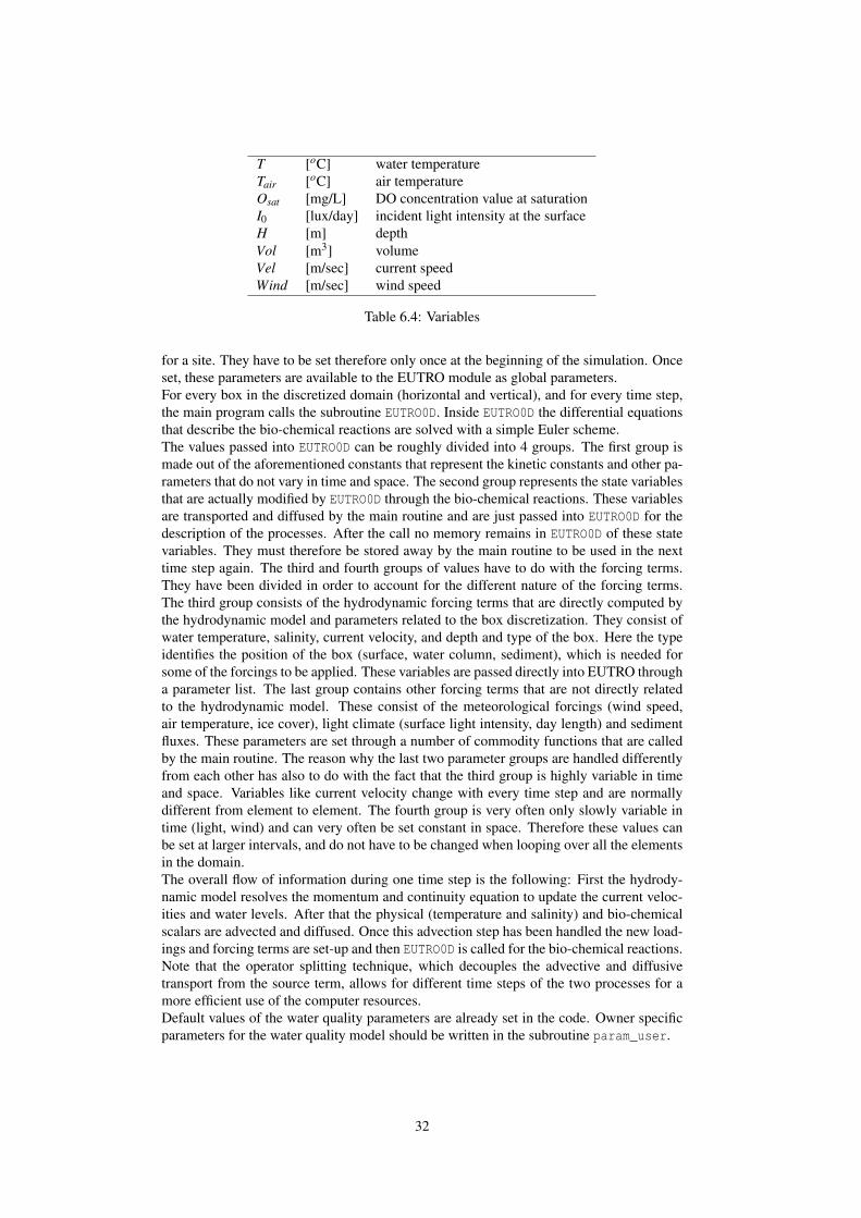
T [oC] water temperatureTair [oC] air temperatureOsat [mg/L] DO concentration value at saturationI0 [lux/day] incident light intensity at the surfaceH [m] depthVol [m3] volumeVel [m/sec] current speedWind [m/sec] wind speed

Table 6.4: Variables

for a site. They have to be set therefore only once at the beginning of the simulation. Onceset, these parameters are available to the EUTRO module as global parameters.For every box in the discretized domain (horizontal and vertical), and for every time step,the main program calls the subroutine EUTRO0D. Inside EUTRO0D the differential equationsthat describe the bio-chemical reactions are solved with a simple Euler scheme.The values passed into EUTRO0D can be roughly divided into 4 groups. The first group ismade out of the aforementioned constants that represent the kinetic constants and other pa-rameters that do not vary in time and space. The second group represents the state variablesthat are actually modified by EUTRO0D through the bio-chemical reactions. These variablesare transported and diffused by the main routine and are just passed into EUTRO0D for thedescription of the processes. After the call no memory remains in EUTRO0D of these statevariables. They must therefore be stored away by the main routine to be used in the nexttime step again. The third and fourth groups of values have to do with the forcing terms.They have been divided in order to account for the different nature of the forcing terms.The third group consists of the hydrodynamic forcing terms that are directly computed bythe hydrodynamic model and parameters related to the box discretization. They consist ofwater temperature, salinity, current velocity, and depth and type of the box. Here the typeidentifies the position of the box (surface, water column, sediment), which is needed forsome of the forcings to be applied. These variables are passed directly into EUTRO througha parameter list. The last group contains other forcing terms that are not directly relatedto the hydrodynamic model. These consist of the meteorological forcings (wind speed,air temperature, ice cover), light climate (surface light intensity, day length) and sedimentfluxes. These parameters are set through a number of commodity functions that are calledby the main routine. The reason why the last two parameter groups are handled differentlyfrom each other has also to do with the fact that the third group is highly variable in timeand space. Variables like current velocity change with every time step and are normallydifferent from element to element. The fourth group is very often only slowly variable intime (light, wind) and can very often be set constant in space. Therefore these values canbe set at larger intervals, and do not have to be changed when looping over all the elementsin the domain.The overall flow of information during one time step is the following: First the hydrody-namic model resolves the momentum and continuity equation to update the current veloc-ities and water levels. After that the physical (temperature and salinity) and bio-chemicalscalars are advected and diffused. Once this advection step has been handled the new load-ings and forcing terms are set-up and then EUTRO0D is called for the bio-chemical reactions.Note that the operator splitting technique, which decouples the advective and diffusivetransport from the source term, allows for different time steps of the two processes for amore efficient use of the computer resources.Default values of the water quality parameters are already set in the code. Owner specificparameters for the water quality model should be written in the subroutine param_user.

32

6.3 Light limitation

6.3.1 Light attenuation formula by Steele and Di ToroThe well known light limitation function proposed by Steele is given as:

P =IIo

e1− IIo (6.3)

where I is the light intensity and Io the optimal light intensity. P is the limiting functionand takes values between 0 and 1.In this form, P is a function of depth z and of time t (P = P(z, t)) since the light intensitydepends on depth and time (I = I(z, t)). The depth dependence of I can be written as

I(z) = Iie−kz (6.4)

where Ii is the incident light intensity on the surface (still dependent on time) and k is anextinction coefficient. Inserting (6.4) into (6.3) gives the equation

P(z, t) =Ii

Ioe−kze1− Ii

Io e−kz= e

Ii

Ioe−kze

IiIo e−kz

. (6.5)

We now compute the average of P over the water column. This gives

P(t) =1H

Z H

0P(z, t)dz =

e IiIo

H

Z H

0e−kze−

IiIo e−kz

dz.

With the substitution x = e−kz and therefore dx/dz = −ke−kz = −kx the integral can betransformed into

P(t) =e Ii

IoH

Z H

0xe−

IiIo x−1

kxdx =−

e IiIo

kH

Z H

0e−

IiIo xdx.

Solving this integral gives finally

P(t) =e

kH

[e−

IiIo x

]H

0=

ekH

[e−

IiIo e−kz

]H

0=

ekH

[e−

IiIo e−kH

− e−IiIo

]. (6.6)

This is the depth integrated form of the Steele limiting function for instantaneous light.If we want to work with the average light over one day, then equation (6.6) can be easilyaveraged over one day. If T is the averaging period (one day), f the fraction of the day withdaylight and Ii is approximated with a step function, 0 at night and Ia during daytime, thenwe can write

P =1T

ZP(t)dt =

1T

f Te

kH

[e−

IaIo e−kH

− e−IaIo

]=

ekH

f[e−

IaIo e−kH

− e−IaIo

]. (6.7)

Equation (6.7) represents the limiting function given by Di Toro and used in the EUTROprogram of WASP. Therefore, equation (6.7) is just the Steele limiting function, but usingIa, the average incident light intensity over daylight hours instead the instantaneous incidentlight intensity Ii used in the original Steele formula (6.6).

6.3.2 Light attenuation formula by SmithEUTRO uses also a light limitation formula by Smith. In the manual this is given as

P(t) =e

kH

[e−

IiIs e−kH

− e−IiIs

]. (6.8)

33

where now IS is the optimal light intensity which is not a constant but is continuouslyadjourned by the program. Again, Ii is the instantaneous light intensity at the surface.Ii is given as

Ii =πIt2 f

sin(πtf

) (6.9)

between 0 and f (daylight) and Ii = 0 otherwise. Averaging (6.9) over one whole day (0–1)gives

Iiday =

Z f

0

πIt2 f

sin(πtf

)dt = It

and averaging only over daylight hours gives

Iidaylight =

1f

Z f

0

πIt2 f

sin(πtf

)dt =Itf

= Ia.

This shows that It in equation (6.9) is the average light intensity at the surface over onewhole day (ITOT in Eutro) and that Ia = It/ f is the average light intensity at the surfaceover daylight hours. This must be taken into account when the Di Toro formulation is used.Note that in EUTRO the actual formula used is Ia = 0.9It/ f where the parameter 0.9 prob-ably accounts for some losses during the integration. The corresponding variables in EU-TRO are FDAY for f and IAV for Ia.

6.4 InitializationThis section describes the interpolation of data for the initialisation of the model.To create a file with initial conditions the program laplap can be used. The program iscalled as laplap < namefile.dat. This makes a laplacian interpolation of specified datacontained in the namefile.dat. This data file should have the first line empty and sholdcontain two colums containing, respectively, node number and data values for the node.It generates two files, laplap.nos and laplap.dat. The first one can be used to checkif the procedure has been conducted well, creating a map with the plotting procedure (seePostprocessing section). The .dat file name should be given in the section $name of the.str file to initialize the model.You can create initialisation files for temperature, salinity, wind field and biological vari-ables. If you want to initialise the biological model with biological data you should createa single data file merging the 9 data files (one for each variable) using the inputmerge.froutine.

6.5 Post processingThis section shows how to generate derivate variables.The post processing routines elaborate the water quality outputs to generate derivate vari-ables. They allow to generate variables such as averages, (both, in time and in space), sumdifferences, and water quality variables such us Vismara, TRIX and BOD5.The routines and their usage are the following:

nosmaniav.f It generates a file containing, for each node of the spatial domani, aver-age, minimum and maximum values of the specified variable of the whole simulation.

nosmaniqual.f It generates a water quality file from the elaboration of the state vari-able. It computes, for each node, and at each time step a water quality index that can bechosen between two suggested indexes: Vismara QualityV and TRIX a well known qualityindex applied to the water quality definition at coastal seas and estuaries.

34

Class(Var) 1 2 3 4 5O2sat 90-110 70-90 or 110-120 50-70 or 120-130 30-50 <30 or >130BOD5 <3 3-6 6-9 9-15 >15NH3 <0.4 0.4-1 1-2 2-5 <5

Table 6.5: Classification of Water Quality Indices

These indices can be computed using the definitions in Table 6.5 and the following equa-tions:

QualityV = class(O2sat) + class(BOD5) + class(NH3)auxt1 = (phyto/30.)*1000auxt2 = (nh3+nox)*1000auxt3 = (opo4+op)*1000

TRIX = log10(auxt1*o2satp*auxt2*auxt3+1.5)/1.2

nosmanintot.f generates a file of total inorganic Nitrogen as sum of NH3 and NOx

nosdif.f computer for the chosen state variable, the difference between the values attwo times step.

nosdiff.f computer the difference between the variable outputs of two simulations

nosmanibod5.f computes the BOD5 values from the CBOD outputs as:

bod5 = cbod*(1. - exp( -5. * par1 ))+ (64./14.) * nh3 * (1. - exp( -5. * par2 ))

To run one of the postprocessing routine write the name of the routine and enter.

6.6 The Sediment ModuleThe sediment buffer action on the biogeochemical cycles could be very important, espe-cially in the shallow water basins and during the storm surge events.The routine wsedim (introduced in April 2004) aims to address the resuspention/sinkingdynamics of nitrogen and phosphorous. This routine can be switched on and off as neededby the user, setting the bsedim parameter true or false in the bio3d routine. It is calledafter the the eutrophication subroutine.It allows to follow the dynamics of two additional variables, OPsed and ONsed that simu-late the evolution of Nitrogen and Phosphorous detritus in sediment that are not subjectedto advection-diffusion processes.These two variables interact with the Nitrogen and Phosphorous cycle as decribed by theequations in Table 6.6. When the wsedim subroutine is switched on, OP, ON, NH3 andOPO4 are updated at each time step in agreement with those equations.The resuspension is a linear function of the water velocity calculated by the hydrodynamicmodel at each box, as written in Table 6.7. The amount of the sinking nutrients dependson specific prossess parameters, as given in Table 6.7, and on the depth of the underlyingcolumn.

35

∂S∂t = Q(S)sed General Reactor Equation

Q(NH3)sed = NH3res 3 Ammonia NH3 [mg N/L]Q(ON)sed = (ONres−ONsink) 5 Organic Nitrogen ON [mg N/L]

Q(OPO4)sed = OPO4res 6Inorganic Phosphorous

OPO4 [mg P/L]

Q(OP)sed = (OPres−OPsink) 7 Organic Phosphorous OP [mg P/L]

Q(ONsed) = ONsink − ONres−NH3res

1sedSediment Organic Nitrogen

ONsed [mg N/L]

Q(OPsed) = OPsink − OPres−OPO4res

2sedSediment Organic Phosphorous

OPsed [mg N/L]

Table 6.6: Sediment Mass balances

NH3res = Volsed ∗ KNCsed∗KNT (T−T0) ∗ONsed

1 Mineralization of organic nitrogen insediment

ONres = Volsed ∗KNres ∗Fvel ∗ONsed 2 Resuspention of organic nitrogen insediment

ONsink = Vol ∗ (1−exp(−dt/τN))dt

∗ON ∗FPON3 Sink of organic nitrogen from the wa-

ter column

OPO4res = Volsed ∗ KPCsed∗ KPT (T−T0) ∗ OPsed 4 Mineralization of organic phospho-

rous in sediment

OPres = Volsed ∗KPres ∗Fvel ∗OPsed 5 Resuspention of organic phospho-rous in sediment

OPsink = Vol ∗ (1−exp(−dt/τP))dt

∗OP∗FPOP6 Sink of organic phosphorous from

the water column

τN = H/ws 7Time scale for sinking processes oforganic N

τP = H/ws 8Time scale for sinking processes oforganic P

Table 6.7: Sediment functional expressions

36

KNCsed = 0.075 Mineralization of sediment ON rate constantKNT = 1.08 Mineralization of sediment ON rate temperature constantKPCsed = 0.22 Mineralization of sediment OP rate constantKPT = 1.08 Mineralization of sediment OP rate temperature constantKNres = 0.1 Fraction of sediment depth resuspended/dayKPres = 0.1 Fraction of sediment depth resuspended/dayFPON = 0.5 Fraction of particulate organic NFPOP = 0.5 Fraction of particulate organic PFvel = 1 Velocity coefficientws = 10 m/day Sinking velocityT0 = 20 oC Optimal temperature value

Table 6.8: Sediment parameters

Vol [m3] volumeVolsed [m3] sediment volumeH [m] total depth of water columndt [sec] time step

Table 6.9: Sediment variables

6.6.1 Parameters for the Water Quality ModuleCompulsory bio parameters These parameters are compulsory parameters that defineif the water quality module is run and what kind of output is written.

ibio Flag if the computation on the temperature is done. The model writesat each time step the state variable values in the the .bio output file

itsmed Flag if the average, minimum, maximum file of variables bio, salinity,temperature is done. if itsmed=1 the model writes .sav, .tav outputfiles of the corresponding variables.

Boundary conditions Boundary conditions have to be given in a file in every section$bound.

bio2dn File name that contains boundary conditions for concentration of thewater quality state variables. The format is the same as for the fileboundn. The unit of the values given in the second and following col-umn (9 data columns for EUTRO) must the ones of the variable.

Initial conditions Initialization of variables are done by file. The files can be created bythe progam laplap. They have to be given in section $name.

bio File with concentration values of water quality variable to be used forthe initialization.

salttemp

Files with salinity concentration values [psu] and Temperature values[deg C] for the initialization.

conz Files with tracer concentration values [for the initialization.

37

Bibliography

[1] Jan O. Backhaus. A semi-implicit scheme for the shallow water equations for aplica-tion to shelf sea modelling. Continental Shelf Research, 2(4):243–254, 1983.

[2] Kurt C. Duwe and Regina R. Hewer. Ein semi-implizites gezeitenmodell fur wattge-biete. Deutsche Hydrographische Zeitschrift, 35(6):223–238, 1982.

[3] G. Grotkop. Finite element analysis of long-period water waves. Computer Methodsin Applied Mechanics and Engineering, 2(2):147–157, 1973.

[4] B. Herrling. Computation of shallow water waves with hybrid finite elements. Ad-vances in Water Resources, 1:313–320, 1978.

[5] Bruno Herrling. Ein finite-element-modell zur berechnung von Tidestromungen inastuarien mit Wattflachen. Die Kuste, 31:102–113, 1977.

[6] K.-P. Holz and G. Nitsche. Tidal wave analysis for estuaries with intertidal flats.Advances in Water Resources, 5:142–148, 1982.

[7] Michael Kwizak and Andre J. Robert. A semi-implicit scheme for grid point atmo-spheric models of the primitive equations. Monthly Weather Review, 99(1):32–36,1971.

[8] A. Schoenstadt. A transfer function analysis of numerical schemes used to simulategeostrophic adjustment. Monthly Weather Review, 108:1248, 1980.

[9] C. Taylor and J. Davis. Tidal and long wave propagation—a finite element approach.Computers & Fluids, 3:125–148, 1975.

[10] Georg Umgiesser. A model for the Venice Lagoon. Master’s thesis, University ofHamburg, 1986.

[11] Georg Umgiesser and Andrea Bergamasco. A staggered grid finite element model ofthe Venice Lagoon. In J. Periaux K. Morgan, E. Ofiate and O.C. Zienkiewicz, editors,Finite Elements in Fluids. Pineridge Press, 1993.

[12] R. T. Williams. On the formulation of finite-element prediction models. MonthlyWeather Review, 109:463, 1981.

[13] R. T. Williams and O. C. Zienkiewicz. Improved finite element forms for the shallow-water wave equations. International Journal for Numerical Methods in Fluids, 1:81,1981.

38