Should smart investors buy funds with high returns

in the past?¤

Frederic Palomino

Tilburg University and CEPR

and

Harald Uhlig

Humboldt University and CEPR

This version: February 27, 2002

Abstract

Newspapers and weekly magazines catering to the investing crowd often

rank funds according to the returns generated in the past. Aside from satisfy-

ing sheer curiosity, these numbers are probably also the basis on which investors

pick a fund to invest in. In this article, we fully characterize the equilibrium in

a game between a mutual fund manager of unknown ability who controls the

riskiness of his portfolio and investors who only observe realized returns. We

derive conditions under which (i) investors invest in the fund if the realized

return falls within some interval, i.e., is neither too low nor too high, (ii) an

¤We are grateful to Alexei Goriaev for helpful research assistance and to the seminar

audience at INSEAD for helpful comments. Correspondnce: Frederic Palomino, Depart-

ment of Finance, Tilburg University, PO Box 90153, 5000 LE Tilburg, The netherlands, e-

mail: f.palomino@kub.nl, Fax: +31-13-466 32 62. Phone: +31-13-466 30 66. Home page:

http://cwis.kub.nl/»few5/center/STAFF/palomino/.

1

informed fund manager picks a portfolio of minimal riskiness and (iii) an unin-

formed mutual fund manager will pick a portfolio with higher risk, \gambling"

on a lucky outcome, (iv), when the fee structure is endogenous, both types of

manager choose the same fraction-of-fund fee structure.

Our results are consistent with empirical evidence about the lack of persis-

tence of top performance, and about the very wide use of fraction-of-fund fee

structure among mutual funds.

1 Introduction

Newspapers and weekly magazines catering to the investing crowd often produce ta-

bles showing \rat races" of mutual funds. They rank funds according to the returns

generated in the previous year or over a period of several years. Aside from satisfying

sheer curiosity, these numbers are probably also the basis on which investors pick a

fund to invest in. Empirical work shows that °ows in and out of funds are indeed pos-

itively correlated with past performances (see See Ippolito (1992), Sirri and Tu®ano

(1998), Chevalier and Ellison (1997) and Lettau (1997)).

Should smart investors buy funds with high returns in the past? To answer this

question, we shall build on the premise that mutual fund managers di®er in their

ability to generate high returns, and that these abilities are persistent at least in the

short run so that returns in year t can be indicative of performances in year t+1 (See

Grinblatt and Titman (1992), Hendrick, Patel and Zeckhauser (1993), Brown and

Goetzmann(1995) and Carhart (1997)1). In such a situation, mutual fund managers

with asset-based compensation schemes2 are surely aware of the signaling function

of their past performance, and will thus choose their portfolio strategies accordingly.

For the sake of the argument, suppose, that investors always pick the fund which

generated the highest return in the past. Knowing this, a fund manager with an

inferior ability may be tempted to gamble, i.e. to invest in risky portfolios, hoping

to generate the highest return in the crowd. But if that is indeed the case, high past

returns are not indicative of high ability: rather, they indicate high risk and a lucky

outcome. Smart investors should thus avoid the top-performing funds.

The contribution of this paper is not only to make this intuition precise, but to

fully characterize the equilibrium in a game between a mutual fund manager and

investors, when only returns are observable. We assume that mutual fund managers

can be either bad or good, a good manager being informed with a high probability

1Evidence of persistent under-performance seem to be stronger than that of over-performance

2See Khorana (1996, section 2)

3

while a bad manager is informed with low probability. Thus, a good manager realizes

a larger return than a bad manager on average. Mutual fund managers control the

riskiness of their portfolio. The investors observe a realization of the fund return, and

invest in the fund, if it is su±ciently likely that the mutual fund manager is good.

The manager will choose the riskiness of his to-be-observed portfolio return in order

to maximize the chance that the investor will invest with him.

We obtain the following results, summarized in Theorem 1. Under some conditions

on the parameters of our model, the investor will invest in the fund, if the realized

return falls within some interval, i.e., is neither too low nor too high. An informed

fund manager picks a portfolio of minimal riskiness. An uninformed mutual fund

manager will pick a portfolio with higher risk, \gambling" on a lucky outcome.

Furthermore, this type of equilibrium is unique for sets of parameters such that

ex-ante (i.e., before observing the return) investors are better o® not investing in the

active fund. Therefore, our results can be interpreted in the following way. If, ex-ante

investors are better o® not investing in the active fund, then a large return should

always be interpreted as the return of an uninformed manager "gambling" rather

than a sign of good information.

Such results are consistent with those of Carhart (1997) who shows that \the funds

in the top decile di®er substantially each year, with more than 80 percent annual

turnover in the composition. In addition, last year's winners frequently become next

year's losers and vice versa, which is consistent with gambling behavior by mutual

funds".

The paper proceeds as follows. Section 2 discusses related literature. Section 3

provides a simple two-quality model, and provides the key results in theorems 1 and

3. Section 4 provides analyzes a more general framework. Section 5 endogenizes the

fee structure and section 6 concludes.

4

2 Related literature

Our paper is substantially di®erent from the existing literature. In particular, the

upper bound is the novel feature of our paper.

The most related models is that of Huddart (1999). He studies a two-period

model in which, at the end of the ¯rst period, risk-averse investors reallocate their

wealth between two funds after having observed the performance of each fund. It is

shown that in the ¯rst, both an informed and an uninformed fund choose overly risky

investment strategies; and in the second period investors should always invest in the

fund that has realized the higher return in the ¯rst period.

There are several di®erences between Huddart's model and ours. First, Huddart

assumes that portfolios are observable while we do not. Huddart's assumption implies

that he studies a standard signaling model in which some additional information is

given by realized returns. If portfolios are not observable, as in our model, managers'

skills can only be derived from statistical inference. Furthermore, we do not ¯nd the

assumption of observable portfolios very appealing since disclosure is not frequent3

and managers window-dress their portfolio around disclosure dates in practice (see

Lakonishok, Thaler, Shleifer and Vishny (1991), Musto (1999) and Carhart, Kaniel,

Musto and Reed (2001)). Second, Huddart assumes that returns are binomially dis-

tributed. Therefore, it is very \easy" for an uninformed manager to obtain exactly

the same return as an informed manager. Hence, there is not much information an

investor can gather from observed returns.

Other models have studied the game played by mutual fund managers (see, for

example, Chen and Pennachi (1999), Goriaev, Palomino and Prat (2000) and Tay-

lor (2000). However all these model take investors' fund picking rule as exogenous

and study the consequences of such a rule on the game played by fund managers.

Conversely, in our model, investors' picking rule is endogenous.

3In the United States, mutual fund portfolios have to be disclosed semiannually. However, other

countries such as the Netherlands only require disclosure once a year.

5

Other papers such as Das and Sundaram (2002) have focussed on e.g. the fee

structure as a way to signal skills: a good manager uses a performance fee structure

with an appropriate benchmark to signal his quality. In our model, when the fee

structure is endogenous, we show that for some sets of parameters, there exists a

pooling equilibrium, which survives the Cho-Kreps intuitive criterion, such that both

good and bad managers choose a fraction-of-fund fee. The main di®erence between

Das and Sundaram's model and ours is that they assume that a good manager learns

his information before choosing his fee while we assume that he receives his information

after choosing the fee.

The pooling equilibrium with fraction-of-fund fees we ¯nd also provides a rational

for the very extensive use of fraction-of-fund fees (rather than performance fee) in the

mutual fund industry (See Golec(1992) and Elton, Gruber and Blake (2001)).

An other model focussing on the fee structure is the one of Heinkel and Stoughton

who also analyze the interplay between a portfolio manager and an investor: there,

the focus is to extract the right e®ort from the manager by conditioning a continued

relationship on the observed return.

Finally, our model is a special case of problem studied by Crawford and Sobel

(1982) in which a sender (the fund manager in our case) sends a costless (noisy)

signal to a receiver (the investors) who makes inference about the sender's type and

then, choose an action.

On the empirical side, investors' smartness in fund picking has been studied by

Gruber (1996) and Zhen (1999). Both articles show that newly invested money per-

forms better than the entire stock of money invested in actively managed funds.

However, newly invested money in actively managed equity funds underperforms in-

dex funds. This suggests that investors' ability to select funds is rather limited. Patel

Zeckhauzer and Hendricks (1994) and Massa (1997) show that the fund-picking by

investors is dictated by their position on a relative ranking of funds performances

rather than the absolute value of the return generated by the funds. This lends mild

empirical support to Theorem 1: if returns are already su±ciently high to land you

6

on top of the heap, it does not help to achieve even higher returns4.

3 The Model

We consider a situation in the spirit of Ippolito (1992). The economy contains two

funds, an actively managed fund which charges high \fraction-of-fund" management

fees and an index fund which charges low fraction-of-fund management fees normal-

ized to zero here. Denote c 2 (0; 1) the di®erence in fee and ¹o the expected returnof the index fund.

The manager of the active fund is of good quality with some probability Á > 0

and of bad quality with probability 1¡ Á.There are two periods: 0 and 1. At the beginning of period 0, the manager of the

active fund picks a portfolio, which generates the return

R = ¹+ ¾²; ² » N (0; 1) (1)

If the manager is of good quality, he is informed with probability µg while a manager of

bad quality is informed with probability µb, with µb < µg. If the manager is informed,

then ¹ = ¹i and if the manager is uninformed, then ¹ = ¹u < ¹i. In picking the

portfolio, the mutual fund manager only controls the riskiness ¾ ¸ ¾ > 0 of the

portfolio, i.e., the mutual fund manager cannot reduce the risk in his portfolio below

some positive lower bound, but he can add as much risk as he wants. For simplicity,

we have assumed that the market price of this risk is zero, i.e., that changing the

riskiness of the portfolio does not a®ect its mean return. This is not restrictive in

principle: if there is a market price for risk, rewrite everything in risk-adjusted terms,

i.e., do a change of measure so that assets can be compared by comparing their

expected returns only, using the new measure. Of course, while this is a standard

and elegant procedure in theory, it may makes comparisons to the data tricky.

4We are grateful to Massimo Massa for pointing this out to us.

7

In order to make the problem interesting, we assume that

(1¡ c)(µb¹u + (1¡ µb)¹i) < ¹o < (1¡ c)(µg¹i + (1¡ µg)¹u)

That is, if the manager is good, the net expected return from investing in the active

fund is larger than the expected return from investing in the index fund. Conversely,

if the manager is bad, the expected return from investing in the active fund is smaller

than that from investing in the index fund.

Note that we may have ¹u = ¹o. In such a case, an uninformed manager does not

underperform an index fund, but charges a larger management fee.

There is a continuum of identical risk-neutral investors. At the end of period 0,

investors only observe the return, but not the choice ¾ or the quality of the manager.

On aggregate, investors have K1 units of capital to invest at the beginning of period

1.

Investors' problem

Given that all investors have the same information, they make the same decision.

Investors choose the actively managed fund if they expect to earn a higher return

after fees than with the index fund. I.e., if investors observe a return R realized by

the actively managed fund, they invest in this fund if

(1¡ c) fP (\good"jR)[µg¹i + (1¡ µg)¹u] + P (\bad"jR)[µb¹i + (1¡ µb)¹ug > ¹o (2)

This is equivalent to

P (\good"jR) > ¹o ¡ (1¡ c)[µb¹i + (1¡ µb)¹u](1¡ c)(µg ¡ µb)(¹i ¡ ¹u)

(3)

We also have

P (¹ijR) = P (¹ij\good")P (\good"jR) + P (¹ij\bad")P (\bad"jR)= µgP (\good"jR) + µbP (\bad"jR)

Therefore,

P (\good"jR) = P (¹ijR)¡ µbµg ¡ µb

8

Using equation (4), we deduce that investors invest in the actively managed fund

if

P (¹ijR) >¹o ¡ (1¡ c)¹u(1¡ c)(¹i ¡ ¹u)

(4)

Let

¿ =¹o ¡ (1¡ c)¹u(1¡ c)(¹i ¡ ¹u)

(5)

Investors will choose to invest in the actively managed fund if the probability that

the fund manager is informed exceeds some treshold ¿ 2 (0; 1).

The fund manager's problem

We assume that the manager of the active fund is risk neutral and his objective is to

maximize his expected revenue over periods 0 and 1. Denote K0, the size of the fund

at the beginning of period 0. 5 After knowing whether he is informed (x = i) or not

(x = u) in period 0, the expected revenue of a manager of type y = g; b is

Rev(c; x; y) = c fK0¹x +K1P [P (¹ijR) > ¿ j¹ = ¹x] (µy¹i + (1¡ µy)¹u)g

Hence, after having set c and knowing whether he is informed, the objective of

the active fund manager is to maximize the probability that investors will choose the

active fund rather than the passive index fund. (The fee charged by the active fund

will be endogenized in Section 5.)

We are interested in the sequential equilibria of the game played by the investors

and the fund manager.

This is an extremely simple model aimed at providing a more precise underpinning

of the intuition described in the introduction. For simplicity sake and on purpose,

5Here, we are considering an active fund manager who has not yet derived a reputation. So, K0

should be viewed as small with respect to K1 (i.e., the amount of money to be invested in period

1). The main objective of the manager is to signal good quality through the realized return so that

investors choose to invest in the active fund at time 1.

9

the model ignores some potentially important aspects. First, the rather mechanical

decision by the investors shortcuts a much lengthier derivation of the portfolio choice

based on ¯rst principles in some multiperiod, multifund model. Such a derivation

would likely complicate the analysis in an unnecessary way.

Second, we have completely ignored an important multiperiod aspect investors

should take into account: the manager will have an incentive to signal good quality

also in the future, using the investors resources to do so. The latter provides for

additional interesting interactions which we hope to analyze in future work.

We analyze the game backwards, searching for the equilibrium (pure-strategy)

portfolio risks ¾¤i and ¾¤u, to be picked by the informed manager and the uninformed

manager, respectively, and the fund picking rule for the investors.

In the last stage of the game, having observed the realized return R and in knowl-

edge of the equilibrium strategies (¾¤i ; ¾¤u), the investors can calculate the likelihood

ratio L(R; ¾¤i ; ¾¤u), that the manager is informed,

L(R;¾¤i ; ¾¤u) =

P (R j ¹i)P (R j ¹u)

=¾¤u¾¤ie(R¡¹i)

2=(2¾¤2i )¡(R¡¹u)2=(2¾¤2u )

Using Bayes rule, the probability of an informed manager having realized the return

R computes to

P (¹i j R) =P (R j ¹i)P (¹i)

P (R j ¹u)P (¹u) + P (R j ¹i)P (¹i)

=Ã

à + (1¡ Ã)L(R; ¾¤i ; ¾¤u)

with

à = Áµg + (1¡ Á)µb

Given that investors invest in the fund if P (¹i j R) ¸ ¿ (see Equations (4) and

(5)) and given the equilibrium strategies (¾¤i ; ¾¤u), the fund will now pick ¾ so as to

10

maximize his chances of receiving investors,

max¾P (

Ã

à + (1¡ Ã)L(R; ¾¤i ; ¾¤u)¸ ¿ ); (6)

where the return distribution of R depends both on ¾ as well as on the information

of the manager via the mean ¹i or ¹u. (See equation (1).)

Therefore, a strategy pair (¾¤i ; ¾¤u) is an equilibrium, if and only if

¾¤x = argmax¾P (Ã

à + (1¡ Ã)L(R;¾¤i ; ¾¤u)¸ ¿) s.t. R = ¹x + ¾²; ² » N (0; 1)

for x = i; u.

We are now ready to state our main results.

Theorem 1 There exists ¹½ < 1 such that if the parameters ¹i; ¹u; ¹o; c; ¾; µg; µb; Á

satisfy

0 > log

µÃ(1¡ ¿ )(1¡ Ã)¿

¶> Max

µ¡12

¡ logµ¹i ¡ ¹u¾

¶; log(¹½)

¶(7)

with

¿ =¹o ¡ (1¡ c)¹(1¡ c)(¹i ¡ ¹u)

; à = Áµg + (1¡ Á)µb

then,

(i) there exists an equilibrium (¾¤i ; ¾¤u) with the following features:

1. An informed manager picks the minimal feasible risk level, ¾¤i = ¾.

2. An uninformed manager picks a risk level, which is strictly greater than the

feasible minimum, ¾¤u > ¾.

3. The investor invests in the fund, if the return R falls in the interval [Rl; Rh] for

some bounds Rl; Rh solving some quadratic equation, and satisfying

¹u < Rl < ¹i < Rh < 1

11

(ii) There is no equilibrium, in which the smart investor will invest if R ¸ R for

some R.

Proof: See Appendix

The following two theorems provide investors' equilibrium investment decisions

for other sets of parameters.

Theorem 2 Suppose, the parameters ¹i; ¹u; ¹o; c; ¾; µg; µb; Á satisfy

(¹i ¡ ¹u)22¾2

> log

µÃ(1¡ ¿)(1¡ Ã)¿

¶: (8)

Then, part (i) of Theorem 1 holds.

Proof: See Appendix.

Theorem 3 Suppose, the parameters ¹i; ¹u; ¹o; c; ¾; µg; µb; Á satisfy

log

µÃ(1¡ ¿)(1¡ Ã)¿

¶>(¹i ¡ ¹u)22¾2

(9)

Then there exists an equilibrium (¾¤i ; ¾¤u) with the following features:

1. Both managers pick the minimal feasible risk level, ¾¤i = ¾¤u = ¾.

2. The investor invests in the fund, if the return R is larger than some threshold

R with

R =¹i + ¹u2

¡ ¾2

¹i ¡ ¹ulog

µÃ(1¡ ¿)(1¡ Ã)¿

¶� ¹u (10)

Proof: See Appendix

Theorem 1 derives conditions under which the realization of a high return signals

that the manager was uninformed and chose a large variance. Since this strategy is

12

more likely to be played by a bad manager (since µb < µg), a rational investor should

not invest in the active fund in period 1.

The interpretation of Theorem 1 is then the following. The ¯rst inequality of

(7) means that ex-ante (i.e., before observing the return) investors are better o® not

investing in the active fund. The theorem says that in such a case, a large return

should always be interpreted as the return of a bad uninformed manager "gambling"

for a lucky outcome, rather than a sign of good information. Such a result is consistent

with those of Carhart (1997) on the lack of persistence of top performance and on

the gambling behavior of mutual fund managers.

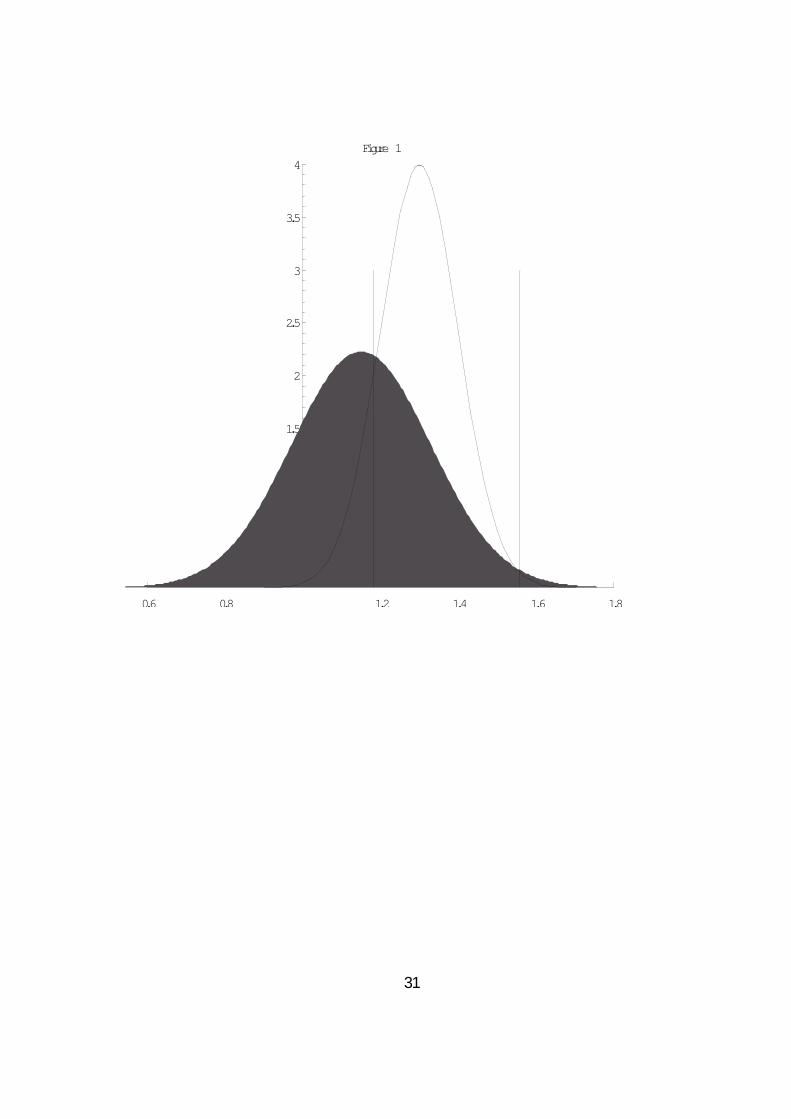
Figure 1 illustrates the results of Theorem 1. The grey area and the bell-shaped

line represent the densities of return generated by an uninformed fund manager and

an informed fund manager, respectively. The two vertical lines represent the lower

and the upper bound (i.e., Rl and Rh) for realized returns between which investors

decide to invest in the fund.

[Insert Figure 1]

The di®erence between Theorems 1 and 2 is that if the ¯rst inequality of (7) does

not hold (but (8) holds), there also exists an equilibrium such that investors always

invest in the active fund no matter what return is observed. This equilibrium is

discussed in Appendix 8. Such an equilibrium does not exists under the conditions

of Theorem 1

The equilibrium proposed by Theorem 3 is more \conventional": pick the fund

which generates the highest returns. The inequality 9 thus provides the dividing line

between a \naive" and a \sophisticated" reading of mutual fund return rankings.

Such fund picking strategy should be implemented when di®erence between good and

bad managers is small (inequality (8) does not hold).

From Theorem 1, we also derive some testable implications for young funds which

have not yet derived a reputation, and mainly aim at attracting new money:

13

² The risk-return relation is U-shaped: top and very bad performance are theresult of high risk portfolio while intermediate performances are the result of

low risk portfolio.

² For top performers, the correlation between performances in two consecutiveyears is negative.

² For good (but not top) performers, the correlation between performances in twoconsecutive years is positive.

4 The general case

The preceeding section concentrated on the highly restrictive case, that there are only

two types of information for the manager. We shall now proceed to the general case

of fairly arbitrary a priori expected returns. Our aim is now more modest: we want to

state su±cient conditions under which we can rule out, that a smart investor should

always pick the fund with the highest return, i.e. we want to state conditions, under

which the answer to the question in the title is negative.

Assume, that the information of the manager is measured by the mean return ¹ he

can achieve, which is drawn according to some prior probability measure ¼(d¹) with

compact support [¹; ¹¹]. The manager picks ¾ within a given interval [¾; ¹¾], 0 < ¾ < ¹¾

and realizes the return

R = ¹+ ¾²

where ² » N(0; 1). The investor observes R and forms posterior beliefs ¼R for the

managerial quality ¹. He will invest in the fund i®

(1¡ c)E¼R[¹] ¸ ¹o

Our general result is as follows.

14

Theorem 4 Suppose that, a priori,

(1¡ c)E¼[¹] < ¹o

Then, for ¹¾ su±ciently large, there is no equilibrium, in which the smart investor will

invest if R ¸ R for some R.

Proof: See Appendix

The theorem generalizes the result of Theorem 1 part (ii): whenever it is not a

good idea to buy the active fund a priori, then investors should always interpret very

large returns as a sign of a bad fund gambling rather than the sign of good ability.

5 Endogenous fee structure

In the previous sections, it was assumed that the fee structure is given: the active fund

charges a fraction-of-fund type of fee. One might be concerned that the fee structure

o®ers managers another avenue for signalling the type, thus undermining the results

obtained above. Indeed, this is exactly what happens in Das and Sundaram (2002).

They assume, however, that the fee structure is chosen after the manager has learned

whether he is informed or not.

By contrast, assume here that the manager has to choose the fee charged to

investors before knowing whether he will be informed (i.e., when choosing the fee

structure, a manager of type x = g; b only knows with that he will be informed with

probability µx). In what follows, we will show that pooling equilibria exist for a

range of parameters: in these equilibria, a good and a bad fund both charge the same

fraction-of-fund fee.

The result in this section is meant to show that the mere possibility of signalling

the type with the fee structure does not by itself imply that this method of signalling

will be employed, and that the analysis above might still be applicable, i.e., Theorem

15

1 is robust to the possibility of signalling with incentive contracts. While it would

be desirable to ¯nd out, whether or not signalling or pooling is going to be the more

prevalent case to occur, a much more quantitative or empirical analysis would be

needed to provide the answer.

As in Das and Sundaram (2002), we restrict our attention to linear fees allowed by

the 1970 Amendment to the Investment Advisors Act of 1940. That is, we consider

fraction-of-fund fees and linear performance fees which are symmetric around some

chosen index (\fulcrum" fees). Therefore, feasible fees are of the following form

C(®1; ®2; B;R) = ®1R+ ®2(R¡B)

If ®2 = 0, then the active fund charges a fraction-of-fund fee. If ®2 > 0, the active

fund charges a fulcrum fee where B is the chosen benchmark return.

We obtain the following result about the possibility of pooling equilibria.

Theorem 5 Assume that the fund manager chooses the fee structure before knowing

before whether his expected return is ¹i or ¹u. Then, there exist sets of parameters

such that there exists a pooling equilibrium in which managers choose a fraction-of-

fund fee structure (i.e., ®1 > 0 and ®2 = 0), and Theorem 1 holds.

Proof: See Appendix

6 Conclusion

This paper provided a simple, highly stylized theory of the game played between

a mutual fund manager and a collection of investors. The mutual fund managers

can be either bad or good, and is thus able to realize either a low or a high return

on investment on average. The mutual fund managers controls the riskiness of his

portfolio; the investors observe a realization of the fund return, and invest in the fund,

if it is su±ciently likely that the mutual fund manager is good. In such a situation,

16

the manager will choose the riskiness of his to-be-observed portfolio return in order

to maximize the chance that the investor will invest with him.

We obtained the following results. Under some conditions on the parameters of

our model, the investor will invest in the fund, if the realized return falls within some

interval, i.e., is neither too low nor too high. An informed mutual fund manager

picks a portfolio of minimal riskiness. A uninformed mutual fund manager will pick

a portfolio with higher risk, \gambling" on a lucky outcome. Thus, smart investors

may not want to buy the fund with the highest returns in the past.

This equilibrium holds for sets of parameters such that ex-ante (i.e., before observ-

ing the return) investors are better o® not investing in the active fund. Therefore, our

results can be interpreted in the following way. If, ex-ante, investors are better o® not

investing in the active fund, then a large return should always be interpreted as the

return of an uninformed manager "gambling" rather than a sign of good information.

Our results on portfolio selection by fund managers are consistent with those of

Carhart (1997) on the lack of persistence in performances by mutual funds. Hence,

investment advisors making recommendations on the basis of funds' past returns

should tell investors to choose a good performer but not a top performer.

17

7 Appendix

Proof of Theorem 1

Proof of (i): The proof proceeds in several steps. We concentrate on ¯nding equilibria,

satisfying ¾¤i � ¾¤u. We will make ample use of this inequality, which obviously needs

to be veri¯ed in the end.

1. The investment decision of the investors.

Given (5), the criterion (4) can be written as

(R ¡ ¹i)2=(2¾¤2i )¡ (R ¡ ¹u)2=(2¾¤2u ) � log

µ¾¤u¾¤i

Ã(1¡ ¿)(1¡ Ã)¿

¶

or, equivalently,

q(R; ¾¤i ; ¾¤u) � 0 (11)

where q(R;¾¤i ; ¾¤u) is a quadratic function in R, given by

q(R; ¾¤i ; ¾¤u) =

µ1

2¾¤2i¡ 1

2¾¤2u

¶R2 (12)

¡µ¹i¾¤2i

¡ ¹u¾¤2u

¶R +

µ¹2i2¾¤2i

¡ ¹2u2¾¤2u

¶¡ log

µ¾¤u¾¤i

Ã(1¡ ¿ )(1¡ Ã)¿

¶

Inequality (11) is satis¯ed, i®

R 2 [Rl(¾¤i ; ¾¤u); Rh(¾¤i ; ¾¤u)] (13)

where Rl(¾¤i ; ¾

¤u) ¸ Rh(¾

¤i ; ¾

¤u) are the two solutions to the quadratic equation

q(R;¾¤i ; ¾¤u) = 0 (14)

Let

½ =Ã(1¡ ¿)(1¡ Ã)¿ (15)

A su±cient condition for the (14) to have two real solutions is that

¢ =

µ¹i¾¤2i

¡ ¹u¾¤2u

¶2

+

µ1

2¾¤2i¡ 1

2¾¤2u

¶�µ¹2u2¾¤2u

¡ ¹2i2¾¤2i

¶+ log

µ¾¤u¾¤i½

¶¸> 0

(16)

18

Let

g(¾i; ¾u) =

µ1

2¾2i¡ 1

2¾2u

¶log

µ¾u¾i½

¶

and

g(½) = min(¾i;¾u);¾u¸¾if(¾i; ¾u; ½)

g(½) is continuous in ½ and g(1) ¸ 0. Therefore, by continuity, there exists ¹½ < 1

such that if ½ > ¹½, then ¢ > 0 and (14) has two real solutions. Furthermore,

we note that for ¾¤i = ¾¤u, the coe±cient on the lead quadratic term becomes

zero. The solutions then take the form

Rh = 1

Rl = R(¾¤i )

where

R(¾¤i ) =¹i + ¹u2

¡ ¾¤2i¹i ¡ ¹u

log

µÃ(1¡ ¿ )(1¡ Ã)¿

¶(17)

2. A ¯rst-order condition for the fund manager.

With (13), the objective (6) of the fund manager with quality x = i; u can be

rewritten as

max¾f(¾;¾¤i ; ¾

¤u) (18)

where f(¾; ¾¤i ; ¾¤u) is the integral

f(¾; ¾¤i ; ¾¤u) =

Z Rh(¾¤i ;¾

¤u)

Rl(¾¤i ;¾

¤u)

1p2¼¾

e¡(R¡¹x)2=(2¾2)dR

To ¯nd the optimum, it is useful to di®erentiate f with respect to ¾,

df

d¾=1

¾I(¾;Rl(¾

¤i ; ¾

¤u); Rh(¾

¤i ; ¾

¤u))

where I(¾;Rl; Rh) is the integral

I(¾;Rl; Rh) =

Z Rh¡¹x¾

Rl¡¹x¾

(²2 ¡ 1) 1p2¼e¡²

2=2d² (19)

19

Standard results about normal distributions imply immediately that

I(¾;¡1;1) = I(¾; 0;1) = I(¾;¡1; 0) = 0 (20)

Furthermore, note that the integrand (²2 ¡ 1) in (19) is negative if j ² j< 1.

These relationships will prove useful in the next step.

3. When do we have ¾¤i = ¾?

From the preceeding analysis, we see that (18) is solved at ¾ = ¾, if

I(¾;Rl(¾¤i ; ¾

¤u); Rh(¾

¤i ; ¾

¤u)) < 0

for all ¾ ¸ ¾. With (20) and the remark following it, it is straightforward

to check, that this is the case if Rl � ¹x � Rh. This in turn is true i®

q(¹x; ¾¤i ; ¾

¤u) � 0. For x = i, this can be rewritten as

q(¹i) = ¡(¹i ¡ ¹u)2

2¾¤2u¡ log

µ¾¤u¾¤i

Ã(1¡ ¿ )(1¡ Ã)¿

¶� 0:

The second inequality of (7) is su±cient for this inequality to hold. This shows,

that ¾¤i = ¾, as claimed.

4. When do we have ¾ < ¾¤u < 1?From the previous step, we deduce that we have an equilibrium with ¾¤i = ¾

and ¾¤u > ¾ if we can rule rule out ¾¤u = ¾ via

I(¾;Rl(¾; ¾); Rh(¾; ¾)) > 0 (21)

and show, that for some ¾ > ¾, we have

I(¾;Rl(¾; ¾); Rh(¾; ¾)) < 0 (22)

An interior solution must then exist by the mean value theorem.

20

Inequality (21) is equivalent to R(¾) > ¹u which is in turn equivalent to the

¯rst inequality of (7). For inequality (22), note that the integrand in equation

(19) is negative for j ² j< 1. Thus, (22) follows, if

¡1 < Rl(¾; ¾)¡ ¹u¾

� Rh(¾; ¾)¡ ¹u¾

< 1

for some ¾. Rewrite this as

¹u ¡ ¾ < Rl(¾; ¾) � Rh(¾; ¾) < ¹u + ¾

which, in turn, is equivalent to

q(¹u ¡ ¾; ¾; ¾) > 0; q(¹u + ¾; ¾; ¾) > 0

for some ¾. However, inspecting (12), it is easy to see that

q(¹u ¡ ¾; ¾; ¾) ! 1

and

q(¹u + ¾; ¾; ¾) ! 1

as ¾ ! 1, completing the proof.

Proof of (ii): We consider the three possible types of equilibria: ¾i < ¾u, ¾i > ¾u and

¾i = ¾u.

Let's consider ¯rst the case ¾i < ¾u. From the proof of Part (i), we know if ½ > ¹½,

then ¢ > 0 and (14) has two real solutions. Hence, there is no equilibrium, in which

the smart investor will invest if R ¸ R for some R.

Consider now the case ¾i > ¾u. Proceeding as in the proof of (i), one obtains that

if the beliefs of the investor are such that ¾¤i > ¾¤u, then the objective of a manager

is to minimize f(¾; ¾¤i ; ¾¤u) over ¾

where f(¾; ¾¤i ; ¾¤u) is the integral

f(¾; ¾¤i ; ¾¤u) =

Z Rh(¾¤i ;¾

¤u)

Rl(¾¤i ;¾

¤u)

1p2¼¾

e¡(R¡¹x)2=(2¾2)dR

21

where x = i if the manager is informed and x = u if the manager is uninformed. It

is straightforward that f(¾; ¾¤i ; ¾¤u) converges to 0 when ¾ goes to +1. Hence, there

is no equilibrium, in which the smart investor will invest if R ¸ R for some R.

Last, consider the case ¾i = ¾u. Assume that the investor's beliefs are such that

¾¤i = ¾¤u. The objective of a manager is to maximize

Prob

µR > ¡ ¾2

¹i ¡ ¹ulog(½) +

¹i + ¹u2

¶

over ¾. From the proof of part (i), we know that a good manager chooses ¾u = ¾.

The condition log(½) < 0 implies that

¡ ¾2

¹i ¡ ¹ulog(½) +

¹i + ¹u2

> ¹u

As a consequence, a bad manager chooses ¾u > ¾. Hence, there is no equilibrium, in

which the smart investor will invest if R ¸ R for some R. 2

Proof of Theorem 2 If Inequality (8) holds then inequality (16) holds. Therefore,

we have the desired result. 2

Proof of Theorem 3 Follow the proof of Theorem 1 above, except for the last step.

Instead of inequality (21), we now get

I(¾;Rl(¾; ¾); Rh(¾; ¾)) < 0 (23)

as a consequence of (9). It follows that ¾¤u = ¾ also. Finally, combine (9) and (10) to

see that R < ¹u. 2

Proof of Theorem 4

Suppose to the contrary, that there was an equilibrium, where the investor always

invests, if R ¸ R for some R. We will show, that there is some R ¸ R (perhaps

22

requiring some su±ciently large ¹¾), so that

E¼R[¹] < ¹¤ (24)

which is a contradiction.

As in the proof of Theorem 1, the fund manager will maximize the probability

that R ¸ R via his choice of ¾. It is easy to check, that he will choose ¾ = ¾, if

¹ ¸ R and ¾ = ¹¾, if ¹ < R. The posterior probability distribution therefore has the

form

¼R(d¹) = Á(R; ¹¾) (mA(d¹;R; ¹¾) +mB(¹;R; ¹¾))

where mA is a measure with support [¹;R) and given by

mA(d¹;R; ¹¾) =1

¹¾exp

µ¡(¹¡R)2

2¹¾2

¶¼(d¹);

where mB is a measure with support [R; ¹¹] and given by

mB(d¹;R; ¹¾) =1

¾exp

µ¡(¹¡R)2

2¾2

¶¼(d¹);

and where Á(R; ¹¾) is chosen so that ¼R is a probability measure.

We now distinguish two cases, R > ¹ and R � ¹.

1. Case: R > ¹

Consider ¯rst the case R > ¹. In that case, the measure ¹A has positive mass,

since ¼(¹ < R) > 0.

Note that the lead term in the exponential expression in mA is ¡R2=(2¹¾2),whereas it is ¡R2=(2¾2) in the exponential expression for mB. Since ¹¾ > ¾, it

follows that mB vanishes relative to mA as R ! 1, ¹¾ ! 1, R=¹¾ ´ const:.

More precisely, for any º > 0, one can ¯nd some su±ently large R as well as

some ~¾, so that for all ¹¾ > ~¾, we have that

j EÁ(R;¹¾)mA(¢;R;¹¾)[¹]¡E¼R[¹] j< º;

23

holding R=¹¾ ´ const. Fix R=¹¾. One can see that

EÁ(R;¹¾)mA(¢;R;¹¾)[¹]! E¼[¹ j ¹ < R]

as ¹¾ ! 1. Put these two pieces together and use

E¼[¹ j ¹ < R)] � E¼[¹] < ¹¤

to demonstrate (24).

2. Case: R � ¹

Next, consider the case R � ¹. In that case, the fund manager will choose

¾ = ¾, regardless of his type ¹. Now suppose that the investor observes R = ¹:

note that he will invest. In that case,

E¼R [¹] =

R¹e¡(¹¡¹)

2=(2¾2)¼(d¹)Re¡(¹¡¹)

2=(2¾2)¼(d¹)� E¼[¹] < ¹

¤;

(where the ¯rst inequality can be seen to hold, since the posterior puts larger

weight on smaller ¹'s), yielding the contradiction. This contradiction does not

require the probability-zero event of exactly observing R = ¹: the inequality

above also remains for R near ¹ by continuity.

2

Proof of Theorem 5

Consider the following set of parameters: Á = 2=3, µg = 0:55, µb = 0:4, ¹i = 1:2,

¹u = 1:16, ¹o = 1:18, ¾ = 0:05, K0 = 0 and K1 = 1. In such a case, à = Áµg +

(1¡ Á)µb = 0:5. If the manager chooses a fraction-of-fund fee structure, then for any®1 > 0, ¿ > 1. Therefore, if ®1 is small enough, the conditions of Theorem 1 are met

while if ®1 is large, the investor never invests in the fund. From Theorem 1, we know

that Rl and Rh are function of the fee charged Therefore, we rewrite them as Rl(®1)

and Rh(®1).

24

Let

rev(®1) = ®1 fK0 +K1Prob [R 2 (Rl(®1); Rh(®1)]g (µg¹i + (1¡ µg)¹u)

and ®¤1 be a solution of

max®1rev(®1) subject to (1¡ ®1)[ùi + (1¡ Ã)¹u] ¸ ¹o

Now, we show that for the set of parameters mentioned above, there exists a

pooling equilibrium in which 1) both types of manager choose a fraction-of-fund fee

(®1 = ®¤1, ®2 = 0) and 2) investors have the following out-of-equilibrium beliefs which

satisfy the intuitive criterion (Cho and Kreps (1987)).

² If the manager chooses a fulcrum fee (i.e., ®2 > 0) with B ¸ ¹¹b = µb¹g + (1 ¡µb)¹b, then the manager is good.

² If the manager chooses a fulcrum fee (i.e., ®2 > 0) with B < ¹¹b, then the

manager is bad.

² If the manager choose a fraction-of-fund fee with ®1 6= ®¤1, then the manager isbad.

First, assume that a bad manager chooses a fraction-of-fund fee with ®1 = ®¤1.

If a good manager chooses a fraction-of-fund fee, he will also choose ®1 = ®¤1 since

it maximizes its revenue among fraction-of-fund fees. Second, assume that a good

manager deviates from the equilibrium strategy and chooses an incentive fee structure

with B ¸ ¹¹b. For this deviation to be pro¯table it must be the case that, given the

incentive fee scheme he chooses, the investor invests in this fund, that is

µg[¹g ¡ ®1¹g ¡ ®2(¹g ¡B)] + (1¡ µg)[¹b ¡ ®1¹b ¡ ®(¹b ¡B)] ¸ ¹o; (25)

It is straightforward that the revenue maximizing incentive fee is a triplet (®1; ®2; B)

such that constraint (25) is binding. Given the set of parameters chosen, the revenue

maximizing incentive fee gives an expected revenue

µg¹g + (1¡ µg)¹b ¡ ¹o = 0:002

25

Now, consider the following fraction-of-fund fee: ®1 = 1 ¡ 1:18=1:19 ¼ 0:0084. In

such a case, ¾u ¼ 0:1685, Rl = 1:1754, Rh = 1:2322, P (R 2 [Rl; Rh]j¹g) = 0:4289

and P (R 2 [Rl; Rh]j¹b) = 0:1294. The expected revenue of a good manager is thenrev(0:0084) = 0:00348. By de¯nition rev(®¤1) > rev(0:0084). This implies that a

good manager has no incentives to deviate from the fraction-of-fund fee ®¤1.

Now, we only need to show that a bad manager never deviates from the equi-

librium. Given the out-of-equilibrium beliefs, a bad manager will never choose a

fraction-of-fund fee with ®1 6= ®¤1 nor an incentive scheme with B < ¹¹b since this

would give zero revenue while playing the equilibrium strategy gives him a strictly

positive expected revenue. The last type of possible deviation is an incentive scheme

with B ¸ ¹¹b. Such a scheme gives a negative expected revenue. Hence, such a devi-

ation is never chosen. This completes the proof.

2

8 Existence of other equilibria under the condi-

tions of Theorem 2

There are also equilibria such that the investor always invests in the fund. Tracing

through the proof above of theorem 1, one can see that such an equilibrium will result,

if

q(R;¾¤i ; ¾¤u) < 0 for all R (26)

In that case, the fund manager is indi®erent between all choices for ¾, regardless of

his type, since his choice does not in°uence the probability of the investor investing

with him. So, any ¾¤i , ¾¤u satisfying (26) is an equilibrium.

Given Ã, ¿ , ¹u, ¹i and ¾, we shall now show, that such ¾¤i and ¾

¤u can always be

found, provided that

log

µÃ(1¡ ¿ )(1¡ Ã)¿

¶> 0 (27)

26

(note that this conditions is assumed to hold also for Theorems 2 and 3). To see this,

¯rst note that (26) requires ¾¤i < ¾¤u. Given this inequality, (26) can be rewritten as

(¹i ¡ ¹u)2 ¡ 2(¾¤i 2 ¡ ¾¤u2) logµÃ(1¡ ¿ )¾¤u(1¡ Ã)¿¾¤i

¶< 0 (28)

after some algebra. Let ³ = ¾¤i =¾¤u: note that we need to keep ³ > 1. Rewrite

equation (28) as

(¹i ¡ ¹u)2 ¡ 2¾¤2u (³2 ¡ 1) logµÃ(1¡ ¿)(1¡ Ã)¿³

¶< 0 (29)

With (27), ¯nd ³ > 1 close enough to 1, so that

log

µÃ(1¡ ¿ )(1¡ Ã)¿³

¶> 0

Next, ¯nd ¾¤u large enough so that inequality (29) is satis¯ed. Calculate ¾¤i = ³¾

¤u to

¯nd an equilibrium of the desired form.

27

References

[1] Bogle, John C., 1992, \Selecting Equity Mutual Funds," Journal of Portfolio

Management, 18(2):94-100.

[2] Brown,S. and W. Goetzmann,1995, \Performance persistence", Journal of Fi-

nance, 50 :679-698.

[3] Brown, K., W., Harlow and L., Stark, 1996, Of tournaments and temptations:

An analysis of managerial incentives in the mutual fund industry, Journal of

Finance, 51:85-110.

[4] Carhart, M., 1997, \On persistence in mutual fund performance", Journal of

Finance, 52:57-82.

[5] Carahrt, M., R. Kaniel, D. Musto, and A., Reed, 2001, \Leaning for the tape:

Evidence of gaming behavior in equity mutual funds", Journal of Finance, Forth-

coming.

[6] Chevalier, J., and G., Ellison, 1997, \Risk taking by mutual funds as a response

to incentives", Journal of Political Economy, 105: 1167-1200.

[7] Cho, I, and D., Kreps, 1987, "signaling games and stable equilibria", Quarterly

Journal of Economics, CII: 179-221.

[8] Crawford, V. and J., Sobel, 1982, '`Strategic information transmission", Econo-

metrica, L: 1431-1451.

[9] Das, S. and R. Sundaram, 2002, \Fee speech: Signaling, Risk sharing, and the

impact of fee structures on investor welfare", Review of Financial Studies, forth-

coming.

[10] Elton, E., M., Gruber, and C. Blake, 2001, \Incentive fees and mutual funds",

mimeo, New York University.

28

[11] Golec, J., 1992, \Empirical tests of a principal agent model of the investor-

investment advisor relationship", Journal of Financial and Quantitative Analysis,

27: 81-95.

[12] Goriaev, A. Palomino, F., and A., Prat, 1998, \Mutual fund tournament: risk

taking incentives induced by ranking objectives", mimeo, Tilburg University.

[13] Grinblatt, Mark and Sheridan Titman,1992, \The Persistence of Mutual Fund

Performance," Journal of Finance, 47: 1977-84.

[14] Grinblatt, Mark and Sheridan Titman, 1993, "Performance measurement with-

out benchmarks: An examination of mutual fund returns", Journal of Business,

66:47-68.

[15] Gruber, Martin J., 1996, \Another puzzle: The growth in actively managed

funds", Journal of Finance, 51: 783-810.

[16] Heinkel, Robert and Neil M. Stoughton, 1994, \The Dynamics of Portfolio Man-

agement Contracts," Review of Financial Studies, 7: 351-87.

[17] Hendricks, D. J. Patel and R. Zeckhauser, 1993, \Hot hand in mutual funds:

Short run persistence of relative performance", Journal of Finance, 48: 93-130.

[18] Hendricks, D. J. Patel and R. Zeckhauser, 1994, Investment °ows and perfor-

mance: evidence from mutual funds, cross-border investments, and new issues",

In Japan, Europe, and International ¯nancial markets: Analytical and empirical

perspectives, Cambridge University Press.

[19] Huddart, S., 1998, \Reputation and performance fee e®ects on portfolio choice

by investment advisers", Journal of Financial Markets, forthcoming.

[20] Ippolito, R., 1992, "Consumer reaction to measures of poor quality: evidence

from the mutual fund industry", Journal of Law and Economics, XXXV: 45-70.

29

[21] Khorana, Ajay, 1996, \Top Management Turnover: An Empirical Investigation

of Mutual Fund Managers," Journal of Financial Economics, 40: 403-27.

[22] Lettau, Martin, 1995, \Explaining the facts with adaptive agents: The case of

mutual fund °ows," Journal of Economic Dynamics and Control, 21: 1117-1147.

[23] Massa, Massimo, 1997, "Do investors react to mutual fund perfomance? An

imperfect competition approach", mimeo, INSEAD.

[24] Musto, D., 1999, \Investment decision depend on portfolio disclosure", Journal

of Finance, 54: 935-952.

[25] Raahauge, P., 1999, Dynamic Programming in Computational Economics, Ph.D.

thesis, University of Aarhus.

[26] Sirri, E. and P., Tu®ano, 1998, \Costly Search and Mutual Fund Flows" Journal

of Finance, 53: 1589-1622

[27] Taylor, J., 2000, \A role for the theory of tournament in studies of mutual fund

behavior", mimeo, MIT.

[28] Zheng, L., 1998, \Is money smart? A study of mutual fund investors' fund

selection ability", mimeo, University of Michigan Business School.

30

0.6 0.8 1.2 1.4 1.6 1.8

0.5

1

1.5

2

2.5

3

3.5

4Figure 1

31