short-term and long-term effects of new light rail transit
TRANSCRIPT
Portland State University Portland State University
PDXScholar PDXScholar
Dissertations and Theses Dissertations and Theses
3-11-2021
Short-term and Long-term Effects of New Light Rail Short-term and Long-term Effects of New Light Rail
Transit Service on Transit Ridership and Traffic Transit Service on Transit Ridership and Traffic
Congestion at Two Geographical Levels Congestion at Two Geographical Levels
Huajie Yang Portland State University
Follow this and additional works at: https://pdxscholar.library.pdx.edu/open_access_etds
Part of the Transportation Commons, and the Urban Studies Commons
Let us know how access to this document benefits you.
Recommended Citation Recommended Citation Yang, Huajie, "Short-term and Long-term Effects of New Light Rail Transit Service on Transit Ridership and Traffic Congestion at Two Geographical Levels" (2021). Dissertations and Theses. Paper 5658. https://doi.org/10.15760/etd.7530
This Dissertation is brought to you for free and open access. It has been accepted for inclusion in Dissertations and Theses by an authorized administrator of PDXScholar. Please contact us if we can make this document more accessible: [email protected].
Short-term and Long-term Effects of New Light Rail Transit
Service on Transit Ridership and Traffic Congestion
at Two Geographical Levels
by
Huajie Yang
A dissertation submitted in partial fulfillment of the
requirements for the degree of
Doctor of Philosophy
in
Urban Studies
Dissertation Committee:
Liming Wang, Chair
Jennifer Dill
Aaron Golub
Wayne Wakeland
Portland State University
2021

© 2021 Huajie Yang

i
Abstract
This dissertation quantitatively examines the effect of new Light Rail Transit
(LRT) services on transit ridership and traffic congestion over time at two different
geographical levels: at the corridor level, this study conducts case studies of two LRT
lines in the Portland, Oregon region; at the regional level, this study uses a synthetic
control method to construct a “synthetic” control Urbanized Areas (UA) that closely
approximates the counterfactual transit ridership and traffic congestion scenario in the
absence of light rail project in three UAs across America. The results of the corridor-level
study suggest that both LRT lines increased transit ridership in the short- and long-term
and relieved traffic congestion in the short-term, while having no statistically significant
effect on traffic congestion in the long-term, likely due to induced traffic demand. Results
of the regional-level study suggest that, while new LRT services contributed to transit
ridership in most UAs, they did relieve traffic congestion in a limited number of UAs,
and that the effect changed over time and varied across UAs. The comprehensively
temporal and geographical analysis will provide a better understanding of the impacts of
new LRT services on transit ridership and traffic congestion, and hence provides policy
makers insightful suggestions for building LRT projects to be more sustainable and to
more effectively attract riders from former auto drivers.

ii
Acknowledgements
I am grateful to many individuals for the completion of this dissertation. Without
the generous support from my adviser, teachers, and mentors along the way, I could not
have turned the research ideas into established research products. As my dissertation
advisor, Dr. Liming Wang, provides enormous support and valuable suggestions. In the
past seven years, he offered me many opportunities to participate in his cutting-edge
research projects. The seven years working with him have been wonderful. I not only
have got comprehensive academic training from him, and also have learned how to be a
rigorous scholar and how to be a good man. He generously shared his time and data and
provided extraordinary patience and guidance to improve my research. I would also like
to send my appreciation to the other professors on my dissertation committee. I would
like to express my gratitude to Dr. Jennifer Dill. It is lucky to take four transportation
courses taught by her. These courses opened the door to the transportation problems and
policies world for me. For my dissertation and field papers, she always gave me very
insightful comments on how to improve. I also want to thank Dr. Aaron Golub. His past
and present research was and continues to be an inspiration for this dissertation. My
discussions with him deepen my understanding of transit and help me to write an
academic paper in a coherent and concise way. I also want to thank Wayne Wakeland.
My discussions with Dr. Wayne Wakeland help me to refine this research and consolidate
the conceptual framework of this research. He also taught me agent-based simulation.

iii
I would also like to thank many other people at PSU. As a field exam committee
member, Dr.Kuan-Pin Lin helped much on the methodologies. He shared the synthetic
control method with me. I would like to thank Dr. Yiping Fang. She always encouraged
and helped me. I shared an office with Dr. Joseph Broach for years and we worked on
one research project. No matter when I have a question and no matter what the question
is, he always could find a solution. He taught me many software techniques and research
skills. I also learned how to do rigorous research from him. For all my peer Ph.D.
Students at the Toulan School of Urban Studies and Planning, thank you for all the years
we have spent together.
Finally, this dissertation is dedicated to my beloved family. I would like to thank
my parents, Ms. Tianhua Lou and Mr. Gaolin Yang, and my elder sister, Ms. Huahui
Yang. Thank you for providing patience, support, and belief in what I was doing. I am
truly grateful. Your full support kept me going through many crises and all-nighters.
iv
Table of Contents
Abstract ................................................................................................................................ i
Acknowledgements ............................................................................................................. ii
List of Tables .................................................................................................................... vii
List of Figures .................................................................................................................. viii
1. Introduction ..................................................................................................................... 1
Research questions .............................................................................................. 4
Conceptual framework ........................................................................................ 6
2. Literature review ........................................................................................................... 14
2.1 Effect of light rail transit service on transit ridership ................................. 14
2.1.1 Corridor level ....................................................................................... 14
2.1.2 Regional level ...................................................................................... 17
2.2 Effect of new transit service on traffic congestion ..................................... 17
2.2.1 Corridor level ....................................................................................... 18
2.2.2 Regional level ...................................................................................... 20
2.3 Induced travel demand ................................................................................ 23
2.4 Gaps in existing literatures.......................................................................... 25
3. Effect of new LRT service on transit ridership and traffic congestion at the corridor
level ................................................................................................................................... 27

v
Research Design ................................................................................................ 28
Data ................................................................................................................... 38
Results ............................................................................................................... 40
Effects on Traffic Congestion ........................................................................... 44
Conclusion ........................................................................................................ 53
4. Effect of new LRT service on transit ridership and traffic congestion at the regional
level ................................................................................................................................... 56
Methodology ..................................................................................................... 57
Data and sample ................................................................................................ 60
Results ............................................................................................................... 63
Charlotte NC-SC ............................................................................................... 63
Transit ridership ............................................................................................ 63
Traffic congestion ......................................................................................... 65
St. Louis MO-IL................................................................................................ 67
Transit ridership ............................................................................................ 67
Traffic congestion ......................................................................................... 69
Virginia Beach VA ........................................................................................... 71
Traffic congestion ......................................................................................... 71
Conclusions ....................................................................................................... 73

vi
5. Discussions and takeaways ........................................................................................... 76
References ......................................................................................................................... 81
vii
List of Tables
Table 2. 1 Empirical studies on the effect of LRT on transit ridership .............................16
Table 2. 2 Corridor studies of transit effect on traffic congestion .....................................19
Table 2. 3 Regional studies of transit effect on traffic congestion ....................................22
Table 3. 1 Transit ridership DID regression models ..........................................................42
Table 3. 2 Crosstab of boardings within the experimental and control corridors ..............43
Table 3. 3 The difference-in-difference base regression models on the speed effect of the
Orange Line .......................................................................................................................46
Table 3. 4 The difference-in-difference base regression models on the speed effect of the
Green Line .........................................................................................................................47
Table 3. 5 Travel Speed Difference-in-Difference Regression Models with Multiple
Time periods on the speed effect of the Orange Line ........................................................50
Table 3. 6 Results of Travel Speed Difference-in-Difference Regression Models with
multiple time periods of the Green Line Case ...................................................................52
Table 4. 1 Control urban areas ...........................................................................................61
Table 4. 2 Selected Treated UAs .......................................................................................63
Table 4. 3 GSCM Results across all three UAs .................................................................73
viii
List of Figures
Figure 1. 1 Conceptual framework of LRT effects on ridership and congestion ................7
Figure 1. 2 The evolution of effect of new LRT service on traffic congestion ...................9
Figure 3. 1 Routes and stations of the MAX Light Rail system in Portland, Oregon
(Source: TriMet Website) ..................................................................................................29
Figure 3. 2 Causal effects in the Difference in Difference model .....................................30
Figure 3. 3 Experimental and control corridor for the Green Line ....................................31
Figure 3. 4 Experimental and control corridor for the Orange Line ..................................31
Figure 3. 5 Population density along I-205 and I-5 ...........................................................33
Figure 3. 6 Employment density along I-205 and I-5 ........................................................33
Figure 3. 7 Population density along SE McLoughlin Blvd and Powell Blvd ..................35
Figure 3. 8 Employment density along SE McLoughlin Blvd and Powell Blvd ...............36
Figure 3. 9 The change in the average weekday boardings at all bus and rail stops located
within the experimental and control corridors over time ...................................................40
Figure 3. 10 The Difference-in-Differences effects of boardings ......................................42
Figure 3. 11 The trends of the boardings and alightings at bus stops located within a
quarter-mile radius of the Green and Orange line stations over time ................................43
Figure 3. 12 The weekday peak periods speed comparison between experimental corridor
(McLoughlin Blvd) and control corridor (Powell Blvd) for the Orange line ....................45
Figure 3. 13 The weekday peak periods speed comparison between experimental corridor
(I-205) and control corridor (I-5) for the Green line ..........................................................45

ix
Figure 3. 14 The estimated speed based on the DID base models for the Orange line
during weekday peak periods .............................................................................................48
Figure 3. 15 The estimated speed based on the DID base models for the Green line during
weekday peak periods ........................................................................................................49
Figure 3. 16 Predicted speed based on the DID models with multiple time periods for the
Orange line during weekday peak periods .........................................................................51
Figure 3. 17 Predicted Average Travel Speed Based on the DID models with multiple
time periods for the Green Line Case ................................................................................53
Figure 4. 1 TTI in Seattle WA and control UAs ................................................................62
Figure 4. 2 PTAUPT per PPT in Charlotte NC-SC ...........................................................64
Figure 4. 3 TTI in Charlotte NC-SC ..................................................................................66
Figure 4. 4 PTAUPT per PPT in St. Louis Mo-IL .............................................................68
Figure 4. 5 TTI in St. Louis Mo-IL ....................................................................................70
Figure 4. 6 TTI in Virginia Beach VA ...............................................................................72

1
1. Introduction
Over the past decades, there have been a continuing increase in private vehicle
usage and an overall decline in the use of public transit in the United States. The
interesting thing is that, despite the fact that private vehicles are increasingly widely used
with the decline of gasoline price and vehicle production costs, more cities are investing
in costly new public transit systems. In 2015, for example, the total operating expense for
transit was $45.3 billion with over 58.6 billion passenger miles traveled in the U.S.
(APTA, 2017). The main end of public transit is to induce more people transfer their
travel mode from driving to riding transit, and to provide the urban poor easy access to
quality life and job opportunities. Some researchers also suggest mass transit (hereafter
referred to simply as transit) as an effective means to reduce auto dependence and relieve
traffic congestion. Bhattacharjee et al. (2012) found that in Denver, the light rail transit
generally lowered the increase of traffic in the influenced highway zone. Anderson
(2013) found that Los Angeles transit provided more congestion relief benefits than what
previously believed.
Although there are continuous large investments in transit, there is a continuing
debate over its effectiveness in relieving traffic congestion. Proponents of building more
transit argue that transit is more efficient than private vehicles and can reduce auto
dependency and relieve congestion. Opponents of building more transit, however, claim
that transit cannot fulfill these benefits, because it cannot attract enough riders in
automobile-oriented areas and transit accounts for a small share of commuting trips in
most American cities. In addition, transit may potentially increase congestion because

2
bus vehicles take up roadway space and interfere with the traffic due to their frequent
stops. Correspondingly, the findings from a large and growing body of studies examining
the effect of transit on transit ridership and traffic congestion have been inconsistent.
The aim of this study is to provide additional in-depth understanding of the short-
term and long-term effect of new light rail transit (LRT) service on transit ridership and
traffic congestion and explain the conflicting empirical results of existing research. LRT is
a kind of transit mode that lies between subway and bus/streetcar. LRT serves fewer people
than the subway does per ride, but it is less expensive and easier to access than the subway.
Compared with buses, LRT is comfortable and speedy, containing more passengers per
ride. Its unique attributes make LRT a mode of choice for many cities. This study will
estimate the effect of new LRT service on transit ridership and traffic congestion at the
corridor and regional levels, and keep track of the changes of these effects over time. This
study focuses on LRT. A primary reason is that transit with a separate right-of-way is likely
to relieve traffic congestion. Downs (2005) contends that transit can reduce traffic
congestion only when the vast majority of peak-hour commuters take transit with separate
right-of-way. Litman (2014) noted less congestion delay in American cities with a high
share of grade-separated transit as compared to cities without a high share of grade-
separated transit. Another reason is that many cities in the U.S. and elsewhere have tilted
their investment in LRT despite its substantially higher cost compared with other
transportation infrastructure. From 1999 to 2017, nationwide vehicle revenue hours of LRT
service have increased from 3.1 million to 7.5 million (NTD, 2000, 2018), which makes
LRT deserved to be separately explored and evaluated quantitatively.

3
The paper is geographically focused on two different perspectives. At the corridor
level, the MAX Green Line and Orange Line in Portland, OR region are selected as case
studies. For each line, using a quasi-experiment design and transportation data before and
after the operation of new LRT service, this study examines the changes in transit
ridership and speed in a view of relatively long time horizon, which may provide
marginal meaningful enlightenment for existing documents. Specifically, I take the
following steps. First, before/after comparisons are conducted. Then, difference-in-
difference (DID) regression models are estimated for each line to evaluate the effect of
new LRT service on ridership and traffic congestion. Thirdly, the difference in the effects
between these two lines is discussed.
At the regional level, this study investigates the effect of New Starts LRT projects
on transit ridership and traffic congestion in large and very large Urbanized Areas (UAs)
in the U.S. From 1998 to 2015, 60 New Starts LRT projects began operation across 27
UAs, but little is known about the effect of these projects on transit ridership and traffic
congestion. This study conducts empirical analyses of the effect of these projects on
transit ridership and traffic congestion. To build up the comparable “counterfactual”
scenario, I use Synthetic Control Method (SCM), initially introduced by Abadie and
Gardeazabal (2003), to examine what the transit ridership and traffic congestion would
have been in the absence of light rail projects.

4
Research questions
This study attempts to quantify the effects of new LRT service on transit ridership
and traffic congestion at the corridor and regional levels, and the changes of such effects
over time. Specifically, this study aims to tackle the following questions:
1. What is the effect of new light rail transit service on transit ridership and traffic
congestion at the corridor level?
2. What is the effect of new light rail transit service on transit ridership and traffic
congestion at the regional level?
3. How does the effect of new light rail transit service on transit ridership and traffic
congestion change over time at the corridor and regional levels?
The first research question investigates the effects of new LRT service on
ridership and congestion at the corridor level. The operation of new LRT service is
expected to improve the level of transit service and accessibility, therefore it is likely to
increase transit ridership, and eventually relieve traffic congestion by attracting former
drivers to transit. But such effects are likely subject to the condition of local
transportation and land use systems, and the attributes of the LRT project. The effects of
new LRT service highly depend on people’s choice faced with the new launch of transit
option: for one thing, the transit may attract some portion of people living near the
corridor to change travel mode from driving personally to public transit, which may
contribute to the increase of ridership and decline of traffic congestion; for the other,

5
people living outside of the corridor zone may choose to change their routes(in the short-
term) or to move to reside near the corridor(in the long-term), and in these cases,
congestion may not be relieved even though the ridership is boosted.
The second question investigates the effects at the regional level. A significant
effect at the corridor level does not guarantee a significant effect at the regional level. On
the one hand, the effect of a single LRT line at the regional level is likely to be small,
because the new LRT service only constitutes a marginal change of overall transportation
supply at the regional level. On the other, a new LRT line may catalyst changes to a
region’s transportation investment priority toward LRT in particular and transit in
general, which may improve the region’s overall transport efficiency. The literature in the
regional perspective is rare. If a region is undergoing an economic boom, resulting in an
influx of both capital and population, its traffic conditions in the short and middle term
are probably unsatisfactory. The launch of new transit may be able to solve part of the
problem, but the average mitigation effect may not be as significant as that in corridor. In
a city where traffic congestion is getting worse, a new transit option may improve
corridor traffic condition.
The third question explores the changes of these effects over time at the corridor
and regional levels. At the corridor level, induced travel demand may play a role in the
changes of the effects of LRT on ridership and traffic congestion. At the regional level,
induced travel demand may be less detectable, because the effect of the New Starts LRT
project is more likely to take place within localized area. The trends at both corridor and
regional levels are deserved to be discussed, because the comparison of corridor and

6
regional results of certain districts will make the picture clearer. For the region of
metropolitan, it is believed that in the long term, only building up extensive and high-
quality of LRT network through continuous investments in LRT may fundamentally
change travel behavior, lowering auto ownership, making transit become the dominant
travel mode, reducing traffic delay.
Conceptual framework
This study follows the conceptual framework shown in Figure 1.1. The short-term
and long-term effects of LRT service on transit ridership and traffic congestion can be
different due to induced travel demand. Pickerell (2001) defines “short-term” as “the
period during which a household's residential locations as well as the spatial distribution
of economic activity and thus of employment remain fixed”. In other words, I take the
location adjustment of household, employment and activity as long-term induced travel
demand that is different from short-term induced travel demand (e.g. people’s travel route
adjustment without destination change). In the framework as pictured, the residential
location and economic activities spatial distribution are vital to explain the long-term
trends of transit ridership and traffic congestion, so the long-term picture may be
significantly different from the short-term.

7
Figure 1. 1 Conceptual framework of LRT effects on ridership and congestion
In the short-term, new LRT service may increase transit ridership and relieve
traffic congestion at the corridor level. New LRT service typically replaces existing bus
service and tends to improve accessibility and the level of transit service along the
corridor, and the extent of such improvement is subject to existing transportation and land
use systems. The improved accessibility and level of transit service attract transit
ridership from three sources: existing unmet transit demand, former transit passengers,
and former drivers. The ridership from former transit passengers has no net effect on
transit ridership and traffic congestion. Ridership from existing unmet transit demand
leads to increased transit ridership but does not affect traffic congestion. Ridership from
former drivers increases transit ridership and relieves traffic congestion. However,
improved traffic conditions are likely to evoke induced travel demand and reduce the
initial benefit to traffic. As illustrated by Pickerell (2001), “short-term induced traffic”
8
includes diverted traffic that changes its route onto the improved facility, rescheduled
traffic that previously used the facility at a different time, shifts from other modes and so
on.
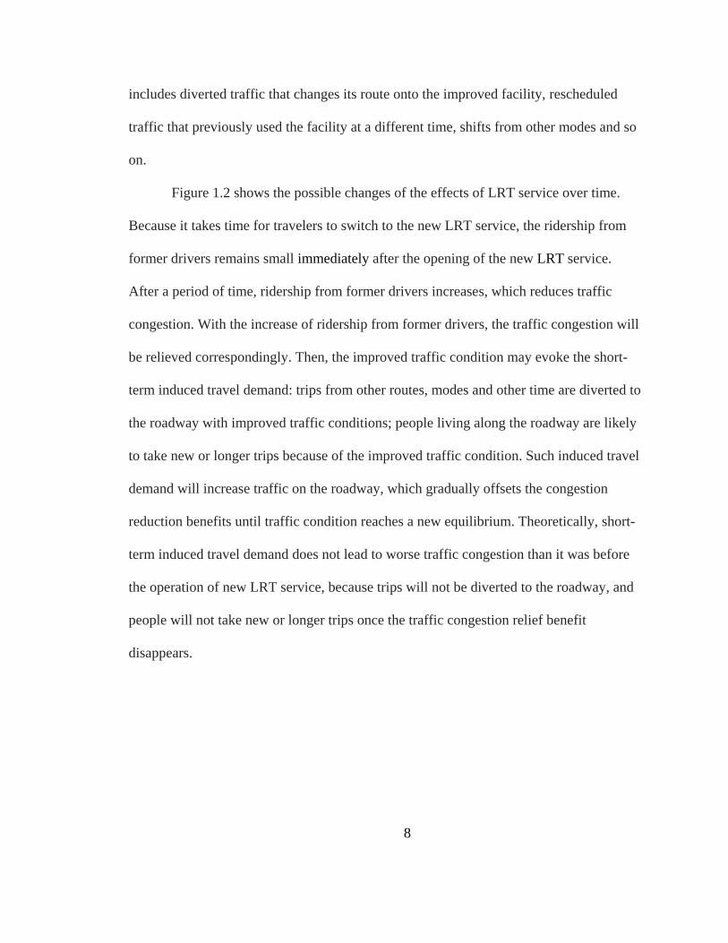
Figure 1.2 shows the possible changes of the effects of LRT service over time.
Because it takes time for travelers to switch to the new LRT service, the ridership from
former drivers remains small immediately after the opening of the new LRT service.
After a period of time, ridership from former drivers increases, which reduces traffic
congestion. With the increase of ridership from former drivers, the traffic congestion will
be relieved correspondingly. Then, the improved traffic condition may evoke the short-
term induced travel demand: trips from other routes, modes and other time are diverted to
the roadway with improved traffic conditions; people living along the roadway are likely
to take new or longer trips because of the improved traffic condition. Such induced travel
demand will increase traffic on the roadway, which gradually offsets the congestion
reduction benefits until traffic condition reaches a new equilibrium. Theoretically, short-
term induced travel demand does not lead to worse traffic congestion than it was before
the operation of new LRT service, because trips will not be diverted to the roadway, and
people will not take new or longer trips once the traffic congestion relief benefit
disappears.

9
Figure 1. 2 The evolution of effect of new LRT service on traffic congestion
In the long-term, new LRT service may increase ridership but worsen traffic
congestion. As mentioned earlier, the operation of new LRT service improves
accessibility along the LRT corridor. The improved accessibility will attract households,
employments, and activities to locate near the LRT stations, leading to increased overall
travel demand. Based on the definition by Pickerell (2001), the induced travel demand
resulting from location adjustment is the long-term induced travel demand. The increased
overall travel demand resulting from long-term induced travel demand may further boost
transit ridership and offset congestion relief benefits or even make traffic conditions
worse than the initial condition.
The effects of new LRT service on transit ridership and congestion are expected
to vary by geographical levels. In the short-term, new LRT service usually constitutes a
marginal change of overall transportation supply at the regional level. Thus, it is expected
10
to exert little influence on transit ridership and traffic congestion at the regional level. In
the long-term, a LRT project may catalyst improvement to the transit system and attract
residents and employments to locate near LRT stations, and eventually leads to detectable
changes in transit ridership and traffic at the regional level. At the regional level, with the
continuing construction of LRT projects, an extensive and high-quality LRT network
may lead to fundamental changes in travel behavior, reducing car ownership and making
transit become the dominant commuting mode, which increases transit ridership, reduces
auto dependence and relieves the traffic congestion at the regional level.
Hypotheses:
1. The effects of new LRT service on transit ridership and traffic congestion at the
corridor level vary by local context.
o The effects of new LRT service on transit ridership and traffic congestion
rely on improving the level of transit service and accessibility along the
transit corridor. The extent of such improvement is subject to existing
transportation and land use system, and existing transportation and land
use system determines transit demand and the extent of current
congestion.
o If the new LRT service primarily attracts ridership from existing transit
riders, it does not affect transit ridership and traffic congestion. If the new
LRT service attracts transit demand that is not met before the operation of
new LRT service, it increases transit ridership and has no effect on traffic
11
congestion. If the new LRT service attracts substantial ridership from
former drivers, which depends on the attractiveness of new LRT service
over driving, it will increase ridership and relieve traffic congestion.
2. The effects of new LRT service on transit ridership and traffic congestion at the
corridor level change over time.
o In the short-term, it takes time for travelers to switch from driving to
riding transit, which may improve traffic condition; then the improved
traffic condition may evoke induced travel demand: trips are diverted
from other routes, modes and times; people living along the corridor take
new or longer trips.
o In the long-term, both people and employment may be attracted to locate
near new LRT stations and land use changes may occur along the LRT
corridor due to improved level of transit service and accessibility, which
further increases transit ridership and worsens traffic congestion
3. The effects of new LRT service on transit ridership and traffic congestion at the
regional level may vary by region.
o Regional socioeconomic factors, state of the economy, and existing
transportation and land use system are all likely to influence the effects at
the regional level.

12
o The effects of new LRT service depend on its scale relative to the
existing system. Single LRT generally has little effect on transit ridership
and traffic congestion at the regional level, because the new LRT service
only constitutes a marginal change of overall transportation supply at the
regional level. An extensive and high-quality LRT network may lead to
fundamental changes in travel behavior, reducing car ownership and
making transit become the dominant commuting mode, and thus can
increase transit ridership and relieve traffic congestion at the regional
level.
4. The effect of new LRT service on transit ridership and traffic congestion at the
regional level changes over time.
o In the short-term, a single LRT project only has little detectable effects
on transit supply, so it has little effect on transit ridership and traffic
congestion at the regional level.
o In the long-term, a LRT project may catalyst improvement to the transit
system and attract residents and employments to locate near transit
station, and eventually leads to detectable changes in transit ridership and
traffic at the regional level. In addition, the construction of extensive and
high-quality LRT network may increase transit mode share and reduce
auto dependence and, therefore, reduce traffic congestion. However, for
the region, decent infrastructure may be accompanied by economic

13
flourish, which probably gives rise to huge marginal traffic demand and
worsens local traffic condition.

14
2. Literature review
The effects of transit include direct effect—transit ridership, and indirect effect,
including traffic congestion, land use, property value, etc. Transit ridership is "a
necessary, but not sufficient condition for any of the indirect benefits ascribed to LRT
investments” (Giuliano et al. 2015). Among the reasons the transit is built to attract
ridership from auto drivers and reduce traffic congestion by virtue of having their rights-
of-way.
2.1 Effect of light rail transit service on transit ridership
As LRT plays an increasingly important role in daily travel, a considerable
amount of studies has examined the effects of new LRT service on transit ridership. In
this review, these studies are grouped by geographical levels: corridor and regional. Table
2.1 summarizes the literature, especially the findings and limitations.
2.1.1 Corridor level
At the corridor level, a stream of studies uses residents as the unit of analysis.
Most of these studies use cross-sectional data, so they only investigate transit ridership at
a single time point. Cervero (1994) examined the transit use of residents living in transit-
oriented development (TOD) areas in California. Results suggested that residents living
close to rail stations were more likely to use transit for both commuting and non-
commuting trips than the average residents in the region. Lund et al. (2006) re-evaluated
the travel pattern of residents living in TOD areas in California and reached similar

15
conclusions. They found that residents living in TOD areas were more likely to ride
transit, especially for commuting, than those who did not live in TOD areas. These two
studies provide evidence about transit usage for daily travel, but they did not use a quasi-
experimental design or take into account residential self-selection (RSS), which might
undermine the validity of their results.
Cao et al. (2014) used a quasi-experimental design and cross-sectional data to
investigate the impact of LRT on transit use. Their analysis examined two urban corridors
and two suburban corridors and used propensity score matching (PSM) to eliminate the
residential self-selection effect on transit use. Results indicated that non-movers, namely
residents living within the LRT corridor before the operation of the LRT, used transit
more frequently than residents in urban control corridors, while movers used transit as
frequently as residents in the urban control corridors.

16
Table 2. 1 Empirical studies on the effect of LRT on transit ridership
Author/s
(years)
Location Unit of
analysis
Data Temporal
Dimension
Key findings Limitations
Cervero
(1994)
California,
USA
Resident Travel
diary
surveys of
targeted
population
Single time
point, 10
years after
transit
service
Stations-
residents
ride rail
transit more
than the
average
residents in
the region
No evidence of
the evolution of
transit ridership;
no quasi-
experimental
design; no RSS
adjustment
Lund et
al. (2006)
California,
USA
Resident Travel
diary
surveys of
targeted
population
Single time
point, 21
years after
transit
service
TOD
residents are
more likely
to use rail
transit than
non-TOD
residents.
No evidence of
the evolution of
transit ridership;
no quasi-
experimental
design; No RSS
adjustment
Cao et al.
(2014)
Minneapolis,
Minnesota,
USA
Resident Travel
diary
surveys of
targeted
population
Single time
point, 7
years after
transit
operation
Non-movers
used transit
more
frequently
than
residents in
the control
corridors,
while
movers used
transit as
frequently as
residents in
the control
corridors
No evidence of
the evolution of
transit ridership
Giuliano
(2015)
Los Angeles,
California,
USA
Corridor Transit
ridership
from
transit
agency
3-month
periods
before and
after transit
service
The Expo
Line has a
net increase
in transit
ridership
Single light rail
line
Baum-
Snow &
Kahn
(2005)
Sixteen
American
cities
City Panel data
set of 16
cities
Time
series,
1970-2000
Rail service
does not
increase
transit modal
share at the
regional
level
An average
effect
Another line of studies uses the transit corridor as the unit of analysis. Giuliano et
al. (2015) investigated the effect of Metro Exposition Line (Expo Line) on transit

17
ridership in Los Angeles, California. Using a quasi-experimental design and a unique
historical archive of high-resolution multimodal transportation data, they examined
transit ridership within the experimental and control corridors before and after the
operation of the Expo Line. Results indicated that the Expo Line increased weekday
boarding of all bus and rail stops within the experimental corridor by approximately
7,000. This study examined only the immediate effects of a single light rail line.
2.1.2 Regional level
Studies examining transit ridership at the regional level are rare. Baum-Snow and
Kahn (2005) examined the effects of rail transit capital investment on public transit
ridership. They used a panel data set of sixteen cities with rail transit improvement
between 1970 and 2000. They found that new rail transit service primarily attracted riders
from bus passengers—not drivers and therefore did not increase transit mode share at the
regional level. Although this study examined the effect of rail transit on ridership over
time with panel data, the estimation is an average effect over time. It did not keep track of
the change of the effect over time.
2.2 Effect of new transit service on traffic congestion
A growing body of studies has examined the effect of transit on traffic congestion,
but the results of these studies are mixed. These studies are also reviewed by
geographical levels: corridor and regional.
18
2.2.1 Corridor level
There has been a considerable amount of literature on the effects of transit
improvement on traffic congestion at the corridor level. The results of these studies are
mixed partly because they are different in terms of measurement, method and time frame,
shown in Table 2.2.
Bhattacharjee et al. (2012) investigated the effect of Denver light rail lines on
traffic congestion from 1992 to 2008. They used Vehicle Miles Traveled (VMT),
converted from Annual Average Daily Traffic (AADT), as traffic performance metric.
Results suggested that light rail lines lowered the growth rate of VMT: the average VMT
within the influence zone increased by 31% compared to 41% outside the influence zone.
Ewing et al. (2014) examined the short-, medium- and long-term effects of the University
of Utah's TRAX LRT line on traffic congestion. They used AADT as the measurement of
traffic congestion and found that LRT reduced AADT in all three time frames. Both
studies suggest that LRT has a congestion relief effect and that effect changes over time,
but they have to approximate their congestion measure from AADT and do not capture
daily or monthly variations in traffic.
In addition to examining transit ridership mentioned above, Giuliano et al. (2015)
investigated the effect of the Los Angeles Metro Exposition Line (Expo Line) on traffic
performance with high-resolution historical archival data. Their results indicated that,
even though it increased transit ridership, it had no significant influence on traffic
congestion. They attributed the insignificant effect on traffic congestion to the large
induced travel demand within the congested corridor. Although this study had a rigorous

19
research design and a sound dataset, a major limitation was that it only examined
transportation performance shortly after the opening of the Expo Line. The Expo Line
began operation in June 2012. They used data during November 2011-January 2012
(before) and November 2012-January 2013 (after) to control the seasonality in their data
and did not examine the medium-and long-term effect.
Table 2. 2 Corridor studies of transit effect on traffic congestion
Author/s
(years)
Location Measurement Temporal
Dimension
Key findings Limitations
Bhattacharjee
et al. (2012)
Denver,
Colorado,
USA
VMT
converted
from AADT
1992 – 2008 LRT lines
decrease the
growth rate
of VMT
within the
influence
zone
No quasi-
experiment;
approximate
measuremen
t of
congestion;
annual
measuremen
t
Giuliano et al.
(2015)
Los
Angeles,
California,
USA
Travel time
and travel time
reliability
3-month periods
before and after
transit service
A net
increase in
transit
ridership; no
significant
influence on
traffic
congestion
No
examination
of
transportatio
n
performance
immediately
before and
after the
opening of
the Expo
Line.
Ewing et al.
(2014)
Salt Lake
City, Utah,
USA
AADT Short-run: 1
year before and
after the
operation of
LRT in 12/2001;
Medium-run:
2001 VS the
average of
2006-2012;
Long-run: long-
run: 1999 VS
2009
LRT reduces
AADT in all
three time
frames.
Congestion
measure is
roughly
approximate
d from
AADT
20
2.2.2 Regional level
Regional studies on the effect of transit on traffic congestion either simulate the
effect with regional travel models, or conduct empirical analysis of transit strike data or
panel data, summarized in Table 2.3. Simulation studies largely build on the assumption
that a subset of transit passengers will switch to driving when transit service is reduced or
halts operation. Therefore, the results of these studies are sensitive to the assumed
proportion of transit passengers switching to driving and all suggest that all types of
transit services can relieve congestion. Nelson et al. (2007) used a regional strategic
planning simulation model to estimate transit service benefits in the Washington, DC
metropolitan area. They found that the transit system reduced a total of 184,000 person-
hours of driving per day, and that rail service generated a larger congestion relief benefit
than bus service. Aftabuzzamand et al. (2010) utilized a regional travel demand model to
estimate the effect of public transit on congestion in Melbourne, Australia. They
converted 32.4% of the public transit trip matrix to the base car trip matrix to simulate a
scenario in which the entire transit system was eliminated. The results indicated that
congestion would increase by more than 150% when the entire transit system was not in
operation.
Simulation studies provide counterfactual insights into what would have
happened if all transit lines halt service, but such studies have pitfalls. The results are
sensitive to the assumed proportion of transit passenger diverting to driving when transit
is not in operation.
21
Transit strike data provide another way to examine what happens when a transit
system halts service Anderson (2013) used a regression discontinuity design to estimate
travel delay with transit labor strike data in Los Angeles, California, and noted a 47%
increase in highway delay during the strike. According to his model, the effect of transit
on traffic volume was minor, but it nevertheless had a large effect on traffic congestion.
Lo and Hall (2006) calculated the average traffic speed during 20 consecutive working
days before and during a transit strike using similar data,. They noted that the length of
the rush period increased by up to 200%. Although such studies provide sound evidence
of the short-term effects of transit on traffic congestion, such studies may not provide
good evidence of response to transit improvement, because travelers are likely to respond
differently to transit improvement and transit cessation. More specifically, travelers must
change travel behavior immediately if transit service is stopped, while travelers gradually
change travel behavior if the level of transit service is improved.

22
Table 2. 3 Regional studies of transit effect on traffic congestion
Author/s (years) Location Methods Time context Key findings Limitations
Nelson et al.
(2007)
Washington,
DC, USA
Simulation
with
strategic
planning
simulation
model
Single time
point
(counterfactua
l analysis )
Rail service
generates
larger
congestion
relief benefit
than bus
services
Implications of
results are limited;
depends on the
proportion of
transit passengers
who convert to
driving; response
to transit cessation
Aftabuzzamand
et al. (2010)
Melbourne,
Australia
Simulation
with travel
demand
model
Single time
point
(counterfactua
l analysis)
Congestion
increased by
more than
150% when
the entire
transit
system was
terminated
Implications of
their results are
limited; depends
on the proportion
of transit
passengers who
convert to driving;
response to transit
cessation
Anderson
(2013)
Los Angeles,
California,
USA
Regression
discontinui
ty
200-day
window
containing the
transit strike
highway
delay
increased by
47%
Response to
transit cessation
Lo and Hall
(2006)
Los Angeles,
California,
USA
Comparati
ve analysis
20 consecutive
working days
before and
after transit
strike
the length of
the rush
period
increased up
to 200%
Response to
transit cessation
Winston and
Langer (2006)
72 UZAs in
the U.S.
Semi-
logarithmic
regression
model
1982 to 1996
(Annual
longitudinal
analysis)
Rail transit
system did
not relieve
congestion
and bus
transit
system
increased
congestion
Estimates are
essentially an
average effect
over time
Beaudoin et al.
(2014)
96 UZAs in
the U.S.
Two-step
GMM
1991- 2011
(Annual
longitudinal
analysis)
A 10%
increase in
overall
transit
capacity
generated on
average
around 0.8%
congestion
reduction
Estimations are
essentially an
average effect
over time

23
Another line of studies utilizes panel datasets to examine the effect of transit on
traffic congestion. Winston and Langer (2006) investigated the effect of highway
spending and transit capacity on VMT with a panel dataset of 72 UZAs over the period
1982 to 1996. They found that rail transit service relieved congestion while bus transit
service increased congestion. Beaudoin et al. (2014) used a two-step Generalized Method
of Moments (GMM) method to examine the effects of transit capacity on traffic
congestion in 96 UZAs across the U.S. from 1991 to 2011. Their results indicated that a
10% increase in overall transit capacity led to on average around 0.8% congestion
reduction. These empirical studies provide weak evidence of the evolution of the effect of
transit on traffic congestion over time, because these estimates with panel datasets are
essentially an average effect over time.
2.3 Induced travel demand
Commonly, induced travel demand refers to the travel demand caused by the
expanded roadway capacity. Many opponents of building more transit for relieving
congestion claim that the addition of transit service also evokes induced travel demand.
Consider a congested roadway. The operation of new transit service reduces the
generalized cost of riding transit by reducing travel time cost, and therefore it may
prompt some drivers to switch to riding transit, which may relieve traffic congestion. The
relieved traffic congestion is expected to evoke induced travel demand at different time
scales.
24
In the short-term, people may take longer trips and/or travel more frequently
taking advantage of the improved traffic, and travel from other routes, times, and modes
may be diverted to the roadway with improved traffic conditions until reaching a new
equilibrium. These induced travel will offset the congestion relief benefit of new transit
service, while it possibly cannot lead to the same or worse traffic congestion than it was
before the operation of new transit service, because travel will not be diverted to the
roadway and people will not take new or longer trips as long as the traffic congestion
relief effect disappear. These conclusions are based on the definition of “the short-term”
as “the period during which household’s residential locations as well as the spatial
distribution of economic activity and thus of employment remain fixed” (Pickerell,
2001).
In the long-term, induced travel demand can cause traffic condition to become
worse than the initial condition. Households and employments are likely to relocate close
to the transit corridor, which may add overall travel demand and make the traffic
congestion worse than before the operation of transit service. An important factor that
should be taken into consideration in the long-term is population growth. Giuliano (2004)
claim that increased travel demand due to population growth is not induced demand.
There has been a large body of empirical studies examining induced travel
demand. Most of these studies focus on the induced travel demand resulting from
roadway capacity expansion (Cervero, 2002; Noland & Lem, 2002). There are limited
studies examining the induced travel demand due to new transit service. Small and
Verhoef (2007, p. 174) noted that the induced auto demand offset the majority of traffic
25
congestion relief benefits of Bay Area Rapid Transit (BART). The operation of BART
attracted 8,750 auto trips to switch to riding transit, but the relieved traffic congestion
evoked 7,000 new auto trips. Beaudoin and Lin (2018) used a panel dataset of 96
Urbanized Areas from 1991 to 2011 to examine the effect of transit supply on auto
demand. Results indicated that the effect of public transit supply on driving demand
change over time due to induced travel demand and substitution effect. A 10% percent
increase in transit supply on average generated a 0.7% decrease in auto demand because
of substitution effect in the short run. Due to induced auto demand offsetting the
substitution effect, transit supply has no effect on auto demand in the medium run. A
10% increase in transit supply on average evoked a 0.4% increase in auto demand in the
long run. They also noted that new transit service could not relieve traffic congestion if
congestion level did not reach a threshold level.
These findings provide supportive evidence for Downs’ (2005) claim that the
traffic congestion relief effect of new transit service is a short-term effect because of
induced travel demand. Induced travel demand resulting from improved traffic
congestion will gradually fill up the roadway space left by auto drivers switching to
riding transit.
2.4 Gaps in existing literatures
A few gaps can be identified in existing studies:
First, the results of existing studies are inconsistent. Several issues seem to
contribute to these inconsistencies: different geographical scales, and variations in terms

26
of data sources, approaches and time periods. The significant effect at the corridor level
cannot guarantee significant effect at the regional level. As mentioned in the literature,
studies using approximate congestion measurement find congestion relief effect while
studies using direct congestion measurement fail to find evidence of congestion relief
effect. Simulation studies indicate all types of transit can relieve traffic congestion, while
empirical studies find conflicting results.
Second, existing studies rarely examine the changes in these effects over time.
Studies using cross-sectional data examine travel behavior at a single time point and
therefore cannot keep track of the changes in these effects over time. Neither can
traditional linear panel data analysis, which estimates elasticities or average change over
time. One exception (as mentioned earlier) is the study by Ewing et al. (2014). They
examined the short-, medium- and long-term effects of LRT on traffic congestion, but
they estimated the effect at three discrete time points rather than tracing the evolution of
the effects. They had to approximate traffic measures from AADT.
Lastly, there are few comparative studies conducted at the regional level. Most
comparative studies are conducted at the corridor level. Comparative analyses are scarce
at the regional level studies probably because it is not easy to find similar control units
for comparison.
27
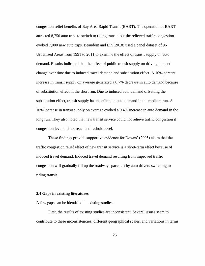
3. Effect of new LRT service on transit ridership and traffic congestion at the
corridor level
Traffic congestion has become an urgent issue across urban areas in the U.S. due
to its direct time and monetary costs and many indirect adverse effects. For instance, the
cost of extra time and fuel due to congestion delay in 498 urban areas has increased from
$24 billion in 1982 to $166 billion in 2017 (Schrank et al., 2019). Besides extra time and
fuel costs, traffic congestion also worsens air quality that causes adverse health effects
and emits additional carbon dioxide and other pollutants which contribute to climate
change (Sun et al., 2019; Yu et al., 2020). To relieve traffic congestion and alleviate its
adverse impacts, light rail transit (LRT), with its separate right-of-way, has been
suggested as an effective means of attracting transit riders from auto drivers and
achieving traffic congestion relief (Downs, 2005; Litman, 2014). So far it still is an
ongoing debate regarding the effectiveness in fulfilling these potentials. Proponents have
argued that it reduces auto dependency and relieving congestion, while opponents have
claimed that LRT either cannot attract enough riders in many automobile-dependent U.S.
cities to matter or, when it does, there is enough latent demand for driving to eliminate
any intermediate effect on the traffic.
Considerable research efforts have been dedicated to examining the actual or
potential effects of LRT on transit ridership and traffic congestion (Bhattacharjee &
Goetz, 2012; Cao & Schoner, 2014b; Ewing et al., 2014; Giuliano, 2004; Litman, 2014).
However, these studies have failed to systematically evaluate both short- and long-term
effects, due to a lack of consistent high-resolution historical data. Partially due to this

28
data limitation, most previous studies on this topic have employed methods strong on
establishing associations; few of them have used methods supporting causal inference.
The purpose of this study is to add to existing research a more in-depth understanding of
the effects of new light rail transit (LRT) service in both short- and long-term timeframe
with a rigorous method supporting causal inference. Through case studies of two LRT
lines in Portland, Oregon, this study conducts two analyses: (1) before and after
comparisons of the LRT opening and (2) the difference-in-difference regression models
to quantify the effects of new LRT service on ridership and traffic congestion. Route-
level transit boarding data and high-resolution historical traffic information from archival
databases and iPeMS enable us to do the analyses. This study expects that this research
fills the research gaps and helps transportation planners, policymakers, and community
members to better understand the effects of LRT on transit ridership and traffic
congestion.
Research Design
Study Area
As the case studies, this study selects the Green Line and Orange Line in the
Portland metropolitan area, where the 59.7-mile MAX light rail system has been built
over three decades partly as a solution to alleviate the worsening traffic congestion.
Figure 3. 1 shows the routes and stations of the MAX light rail system. The two cases are
selected due to the trend in transit ridership and traffic congestion, and the availability of
current and historical ridership and travel speed data for analysis. The Green Line is a 15-
29
mile LRT line opened on September 12, 2009. It extends transit service to the eastside
Portland metropolitan area by connecting Clackamas, Happy Valley, and downtown
Portland. The Orange Line is a 7.3-mile light rail line opened in September 2015, the
latest addition to the MAX light rail system. It extends light rail service to Southeast
Portland, connecting downtown Portland, Portland State University, and Park Avenue in
South East Portland.
Figure 3. 1 Routes and stations of the MAX Light Rail system in Portland, Oregon
(Source: TriMet Website)
Methodology
This study aims to quantify the effects of new LRT lines on transit ridership and
traffic congestion at the corridor level and analyze the changes of these effects over time.
This study uses a quasi-experimental design, and a difference-in-difference (DID)
method with high temporal and spatial resolution data. The DID method is used to
estimate group-level fixed effects of treatment (Figure 3. 2) with an ability to correct

30
group-level omitted variable bias. The following equation shows the classic DID
regression model:
𝑦𝑖𝑡𝑔 = 𝛽0 + 𝛽1𝑇 + 𝛽2𝐺 + 𝛽3𝑇𝐺 + 𝜀
where:
𝑦𝑖𝑡𝑔 = outcome of interest (transit ridership and travel speed) on roadway segment i of
group g
(experimental/control) during time period t (before/after)
T = dummy variable indicating time period (“1” for after the opening)
G = dummy variable indicating treated and control group (“1” for experimental group)
𝛽3 = the DID estimate
Figure 3. 2 Causal effects in the Difference in Difference model

31
Control and Experimental Groups
This study chooses the corridors along a segment of the Green and Orange lines
as experimental groups. This study then selects a control corridor for each line. Figure 3.
3 and Figure 3. 4 show the experimental and control corridors for the Green and Orange
lines.
Figure 3. 3 Experimental and control corridor for the Green Line
Figure 3. 4 Experimental and control corridor for the Orange Line

32
The Green Line provides an additional travel mode between Clackamas and
downtown Portland. This study focuses on the segment of the Green Line that stretches
from Clackamas Town Center Station to SE Main St. Station. This segment of the Green
Line is 7 miles long and runs close and parallel to I-205. After reviewing roadways
profiles and traffic characteristics, I select the I-5 segment south of Downtown Portland
as the control roadway, beginning at the interaction of I-5 with Ross Island Bridge to its
intersection with Oregon Route 99. The Orange Line provides an alternative mode
between downtown Portland and SE Portland.
The chosen I-5 segment and I-205 segment are comparable. I-5 is an interstate
highway. I-205 is an auxiliary interstate highway, serving as a bypass route of I-5. The
traffic volume of the two segments is similar, and they both serve the north-south traffic.
From Clackamas Town Center to the North of Halsey Street, the selected I-205 segment
travels through the eastern residential area of Portland, mainly including neighborhoods:
Lents, Southgate, and West Mt. Scott. From its intersection with Oregon Route 99 to the
north of Downtown Portland, the selected I-5 segment travels the southern residential
area of Portland, mainly including neighborhoods: FAR Southwest, Crestwood, West
Portland Park, Multnomah, Markham, South Burlingame, Hillsdale, and South Portland.
Figure 3. 5 and Figure 3. 6 show that population density and employment density are
similar along I-5 and I-205. Though the selected I-5 segment is a comparable control
roadway, there are still some differences between I-5 and I-205. I-5 directly connects
with Downtown Portland, while I-205 locates far away from the downtown area. The

33
downtown area acts as an important employment center Portland Metropolitan Area.
Thus, there are probably differences in traffic patterns between I-5 and I-205.
Figure 3. 5 Population density along I-205 and I-5
Figure 3. 6 Employment density along I-205 and I-5

34
However, the selected I-5 highway segment is a better option as a control
roadway after reviewing the other roadways in the area. An alternative of control
roadway is Oregon Route 99W. It runs parallel to the I-5 highway. Since it is a state-
numbered route, different from the experimental roadway, it is not selected. Another
choice of control roadway is the I-5 segment from outside of downtown Portland
northbound to Vancouver. However, from its intersection with N Columbia Blvd to
Vancouver, the I-5 segment serves Delta Park, a recreational area. Thus, the I-5 segment
from outside of downtown Portland northbound to Vancouver is not selected as a control
roadway.
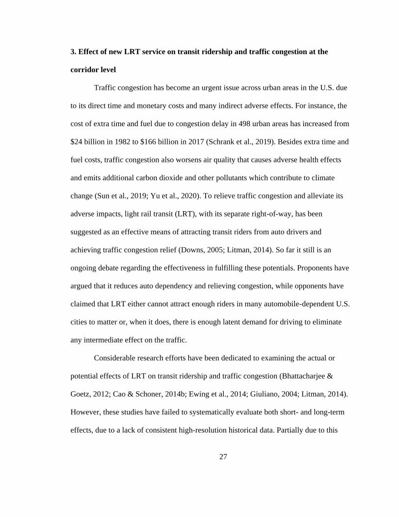
For the Orange Line, the experimental corridor is the area along the SE
McLoughlin Blvd. From downtown Portland to Park Ave in SE Portland, most of SE
McLoughlin Blvd is parallel and close to the Orange Line. The roadway segments within
the experimental corridor include SE McLoughlin Blvd from its intersection with SE
Franklin St to its intersection with SE Park Ave. After examining roadway profile and
traffic characteristics, the control corridor is selected to be the SE Powell Blvd segment
bounded by SE 122th Ave to the east and SE McLoughlin Blvd to the west. The control
corridor is generally perpendicular to the Orange Line, and therefore should not be
affected by the Orange Line.
The selected SE McLoughlin Blvd segment and SE Powell Blvd are comparable.
The SE McLoughlin Blvd is an urban expressway, and it serves the southeastern
residential area, mainly including neighborhoods: Hosford-Abernethy, Brooklyn and
Sellwood-Moreland. SE Powell Blvd is an urban expressway, and it mainly serves the
35
eastern residential area, including neighborhoods: Sullivan’s Gulch, Kerns, North Tabor,
Montavilla, and Centennial. The population density and employment density are similar
along the selected SE McLoughlin Blvd segment and SE Powell Blvd, shown in Figure 3.
7 and Figure 3. 8. The selected SE McLoughlin Blvd segment and SE Powell Blvd are
comparable in an overall sense. An alternative of the control roadway is Oregon Route
99E from North of NE Multnomah Street northbound to Vancouver. The Oregon Route
99E segment serves Delta Park, a recreation area, it is not finally selected.
Figure 3. 7 2010 population density 2010 along treatment (SE McLoughlin Blvd)
and control (Powell Blvd)

36
Figure 3. 8 2010 employment density along treatment (SE McLoughlin Blvd) and
control (Powell Blvd)
Existing research has found the association between transit use and land use
(Cervero, 1994; Ding et al., 2014; Ewing & Cervero, 2010). The transit model would be
improved after including land use variables. This study still does not include land use
variables because of data availability at the corresponding temporal and spatial
resolution. In the transit model, the ridership data are quarterly, while land use variables
are annual. The temporal resolutions are different.
Population density is another variable that should be included in the transit model.
This study does not include this variable due to two issues. The first issue is the temporal
resolution of the population density variable. Population from U.S. Census Bureau is
annual 5-year rolling data, while the transit ridership data are quarterly. The temporal
resolutions are different. Second, in order to include population density in the transit
37
model, it must be assumed that the population is equally distributed. This assumption
does not reflect reality.
Because of lacking land use and population density variables, my estimation of
the effect of the new LRT project on ridership is likely to be biased by overestimating the
effect. Land use and population change are likely to contribute to ridership increase. In
the regression model without land use and population variables, the impact of land use on
ridership would be attributed to the new LRT project. Thus, the impact of the new LRT
project on transit ridership would be overestimated because the coefficients include the
effects resulting from land use and population changes.
Since population and land use changes are similar in the control and experimental
corridors, the DID method used here may make up the impact of not including population
and land use variables in the transit models because the selected control and experimental
corridors are still comparable.
Other changes, such as ramp meters, that affect travel speed on the highway
should also be considered when evaluating the impact of the new LRT project on
congestion if they were implemented on the control or treatment corridor (but not both).
The purpose of ramp meters is to reduce bottlenecks and improve the overall speed of
traffic flow. By regulating vehicles entering a highway, ramp meters can avoid situations
where a large number of vehicles move onto the highway at one time and lead to traffic
congestion. Ramp meters also can improve travel speed by reducing crashes. If ramp
meters are implemented before the operation of the new LRT project, it would not affect
the impact of the new LRT project on traffic congestion. If ramp meters are implemented

38
after the operation of the new LRT project, they will affect the impact of the new LRT
project on traffic congestion. However, no information can be found on the
implementation of such changes to the control or treatment corridor.
Data
This research focuses on the effects of LRT on both transit ridership and traffic
congestion in that the transit ridership effect is a necessary, but not sufficient condition to
explain indirect benefits ascribed to LRT (Giuliano et al., 2015). This study examines
both effects by using transit boarding data and high-resolution historical traffic
information from archival databases and iPeMS to comprehensively investigate the short-
and long-term effects of LRT at the corridor level with case studies of two LRT lines in
Portland, Oregon.
For traffic congestion data, this study uses route-level travel speed as a measure of
traffic congestion. For the Green line case, this study employs the Transportation Data
Archive for Portland-Vancouver (PORTAL) for travel speed data. PORTAL is a
historical multi-modal transportation data archive, including historical weather data,
incident data, transit data, and 20-second granularity loop detector data for the Portland-
Vancouver metropolitan region since July 2004 (Hansen et al., 2005). There are 13 and
11 loop detector stations in the experimental and control corridors, respectively. Each
loop detector installed along the roadways generates a record including volume, speed,
and occupancy for its corresponding lane every 20 seconds. Theoretically, each detector
generates 4,320 records in a single day, but the actual number may be smaller due to non-
39
reporting, which are excluded from this research. The 20-second granularity is sensitive
to random noise, so this study aggregates the data into 5-minute granularity. This study
then converts station-level data to route-level data. The final number of records for travel
speed is 11,482. Because the PORTAL data do not cover arterials, for the Orange line
case, this study uses the iPeMS database for travel speed data, which is an online
database tool provided by Iteris, Inc. The iPeMS database collects probe data from a
sample of data collected from vehicle navigation systems, cell phone apps, and fleet
vehicles. In iPeMS, users have access to statewide travel data from highways, principal
arterials, minor arterials, and major collectors. Users can extract route-level travel data by
assigning origination and destination only as far back as 2011, so it cannot be used for the
Green Line case.
This study utilizes travel speed data collected before and after the operation of the
LRT lines. The Orange Line began operation on September 12, 2015. The travel speed
data were collected for the three year periods before (from September 12, 2012, to
September 11, 2015) and after (from September 12, 2015, to September 11, 2018) the
opening of the Orange Line. The Green Line began operation on September 12, 2009.
The travel speed data were collected for the five-year periods before (from September 12,
2004, to September 11, 2009) and after (from September 12, 2009, to September 11,
2014) the Green Line opening.
This study obtains the data set from TriMet, the transit authority for the Portland,
Oregon region, regarding transit ridership. The data includes boarding and alighting
information by transit line, stop, time of day, and day of the week. The data has been

40
collected by TriMet every three months. The time periods of transit ridership data used in
this study are the same as travel speed data.
Results
Effects on Transit Ridership
Average weekday ridership
First, this study analyzes average weekday boardings at all bus and rail stops
located within the experimental and control corridors before and after the operation of the
two light rail transit lines. As shown in Figure 3. 9, the vertical dashed line indicates the
date when the new light rail transit lines began operation. After the openings, boardings
within each of the experimental corridors noticeably increased, while boardings within the
control corridor decreased slightly for the Orange Line and remained nearly stable for the
Green Line.
Figure 3. 9 The change in the average weekday boardings at all bus and rail stops
located within the experimental and control corridors over time

41
The difference-in-difference regression models
This study then uses the DID regression models to examine the impacts on
ridership. The DID estimators of base models were both statistically significant and
positive, demonstrating that the average treatment effect of new LRT lines is 6,404 and
7,225 for the Orange Line and Green Line, respectively (Table 3. 1). That is, the Orange
Line and Green Line contribute to an increase of 6,404 and 7,225 riders on average,
respectively (Figure 3. 10). Analyzing the ridership by each year after the operation of the
Green Line, results indicate that there was an increase in ridership compared to the
ridership in the control corridor (Table 3. 2). Table 3. 2 shows that ridership increased in
the first year and then remained nearly stable after the first year for the Orange Line. For
the Green Line, the ridership increased to about 9,000 from about 3,000 in the first year,
and to about 9,500 in the second year, then kept relatively stable from the third year
onward, and reached the maximum in the 7th year.
In sum, the DID estimators of both base models confirm the increase in transit
ridership. More importantly, the two LRT lines lead to a large increase in transit
ridership, particularly for the first few years of the operation of new LRT lines. This
study also compares boardings and alightings at bus stops within a quarter-mile network
distance of Orange Line stops before and after the Orange Line operation. The results
also reveal that bus boardings and alightings both increased after the operation of both
LRT lines (Figure 3. 11).

42
Table 3. 1 Transit ridership DID regression models
Variable Orange Line Base
model
Green Line Base
model
Time period (after=1) -554.00***
(179.00)
-102.00***
(196.00)
Group (experimental group=1) -7,662.00***
(189.00)
-821.00***
(260.00)
Time period*Group 6,404.00***
(254.00)
7,225.00***
(277.00)
Constant 13,599.00***
(134.00)
3,716.00***
(184.00)
Observations 54 86
R2 0.98 0.985
Adjusted R2 0.98 0.984
Residual Std. Error 463.00
(df=50)
411.00
(df=82)
F Statistic 712.00***
(df = 3; 50)
1,753.00***
(df = 3: 82)
Note: *p<0.1; **p<0.05; ***p<0.01
Figure 3. 10 The Difference-in-Differences effects of boardings

43
Table 3. 2 Crosstab of boardings within the experimental and control corridors
Orange Line Green Line
Time period Control corridor Experimental
corridor
Control corridor Experimental
corridor
Before 13599 5938 3716 2895
1st year 13289 11799 3671 8960
2nd year 12902 11634 3417 9694
3rd year 13028 11800 3606 10080
4th year 12936 11961 3327 9926
5th year 3556 10030
6th year 3782 10204
7th year 3724 10478
8th year 3683 10144
9th year 3689 10144
10th year 3721 10334
Figure 3. 11 The trends of the boardings and alightings at bus stops located within a
quarter-mile radius of the Green and Orange line stations over time

44
Effects on Traffic Congestion
This study focuses our study on the effects of LRT on traffic congestion on
weekday peak periods when traffic volumes are considerably heavy and congestion more
common: the AM peak between 7-10 AM, and the PM peak between 4-7 PM.
Average speed
This study, firstly, analyzes the average speed on experimental and control
roadways by peak periods and directions (inbound to/outbound from downtown) for the
Orange and Green lines (Figure 3. 12 and Figure 3. 13). For the Orange line case, as
shown in Figure 3. 12, while the trend of average peak period travel speed on the
experimental and control roadway segments was similar before the operation, average
peak periods travel speed for both directions of the experimental corridor increased after
the operation. The increase of speed for AM peak outbound from downtown was the
largest, followed by PM peak inbound to downtown, that is, the directions with less
congestion and higher speed to begin with. For the Green line case, shown in Figure 3.
13, the average peak period travel speed on the experimental and control roadways was
overall similar before the opening of the Green line. After its operation, the average speed
on the experimental roadway saw little change. Also, note that there was a large variation
in travel speed on the control roadway (I-5).

45
Figure 3. 12 The weekday peak periods speed comparison between experimental
corridor (McLoughlin Blvd) and control corridor (Powell Blvd) for the Orange line
Figure 3. 13 The weekday peak periods speed comparison between experimental
corridor (I-205) and control corridor (I-5) for the Green line

46
Difference-in-Difference base regression models
For the Orange line case, the results in Table 3. 3 show that each of the four
models one for each period and direction combination, indicated a significant increase in
the speed, ranging from 1.35 mph to 2.35 mph on average, of the experimental roadway
in all cases. That is, our results suggest that the Orange Line has an effect on increasing
travel speed on the experimental segment. The size of the impacts differed across the
periods and directions.
Table 3. 3 The difference-in-difference base regression models on the speed effect of
the Orange Line
AM Outbound AM Inbound PM Outbound PM inbound
Time Period
(after = 1)
-0.257***
(0.077)
-0.748***
(0.180)
-2.130***
(0.100)
-1.490***
(0.083)
Group
(experimental
group =1)
10.300***
(0.077)
6.690***
(0.180)
9.090***
(0.108)
12.000***
(0.083)
Time period *
Group
2.350***
(0.109)
1.500***
(0.255)
1.350***
(0.152)
2.070***
(0.117)
Constant 23.200***
(0.055)
19.500***
(0.127)
19.700***
(0.076)
21.800***
(0.058)
Observations 3,129 3,130 3,128 3,128
R2 0.935 0.524 0.844 0.941
Adjusted R2 0.935 0.523 0.843 0.941
Residual Std.
Error
1.530 (df =
3,125)
3.570 (df =
3,126)
2.130 (df =
3124)
1.630 (df =
3124)
F Statistic 14,943.000***
(df = 3; 3125)
1,146.000***
(df = 3; 3126)
5,616.000***
(df = 3; 3124)
16,664.000***
(df = 3; 3124)
Note: *p<0.1; **p<0.05; ***p<0.01
For the Green line case, as shown in Table 3. 4, each of the four models indicated
a significant increase in travel speed of the experimental roadway in both directions during
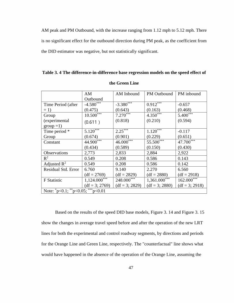
47
AM peak and PM Outbound, with the increase ranging from 1.12 mph to 5.12 mph. There
is no significant effect for the outbound direction during PM peak, as the coefficient from
the DID estimator was negative, but not statistically significant.
Table 3. 4 The difference-in-difference base regression models on the speed effect of
the Green Line
AM
Outbound
AM Inbound PM Outbound PM inbound
Time Period (after
= 1)
-4.580***
(0.475)
-3.380***
(0.643)
0.912***
(0.163)
-0.657
(0.468)
Group
(experimental
group =1)
10.500***
(0.611)
7.270***
(0.818)
4.350***
(0.210)
5.400***
(0.594)
Time period *
Group
5.120***
(0.674)
2.25***
(0.901)
1.120***
(0.229)
-0.117
(0.651)
Constant 44.900***
(0.434)
46.000***
(0.589)
55.500***
(0.150)
47.700***
(0.430)
Observations 2,773 2,833 2,884 2,922
R2 0.549 0.208 0.586 0.143
Adjusted R2 0.549 0.208 0.586 0.142
Residual Std. Error 6.760
(df = 2769)
9.140
(df = 2829)
2.270
(df = 2880)
6.560
(df = 2918)
F Statistic 1,124.000***
(df = 3; 2769)
248.000***
(df = 3; 2829)
1,361.000***
(df = 3; 2880)
162.000***
(df = 3; 2918)
Note: *p<0.1; **p<0.05; ***p<0.01
Based on the results of the speed DID base models, Figure 3. 14 and Figure 3. 15
show the changes in average travel speed before and after the operation of the new LRT
lines for both the experimental and control roadway segments, by directions and periods
for the Orange Line and Green Line, respectively. The "counterfactual" line shows what
would have happened in the absence of the operation of the Orange Line, assuming the

48
change in travel speed on the experimental roadway segment would mirror the change in
travel speed on the control roadway segment. For the Orange Line, the travel speed on
the experimental roadway segment for after period is higher than that in the
counterfactual scenario (Figure 3. 14). For the Green Line, the travel speed on the
experimental roadway segment for the after-period was higher than that in the
counterfactual scenario for the after-period, except in the case of the PM outbound
(Figure 3. 15). I, thus, conclude that both LRT Lines have had a relief effect on travel
speed on the experimental roadway segment.
Figure 3. 14 The estimated speed based on the DID base models for the Orange line
during weekday peak periods

49
Figure 3. 15 The estimated speed based on the DID base models for the Green line
during weekday peak periods
Difference-in-Difference regression models with multiple time periods
This study further investigates how the increase in travel speed changes over time
by applying the DID regression models with multiple time periods. As predicted by the
induced demand hypothesis, the increase in travel speed, if any, would diminish over time.
Table 3. 5 shows the results of the DID regression models with multiple time
periods for the Orange Line case. The results of the DID estimators indicated that the
increases in travel speed of the experimental roadway persist and improve over time, as
most coefficients for Year * Group is significant with magnitude increasing from the 1st
to 2nd and then 3rd year. Two exceptions are the effect on the outbound direction for the
PM period in the first year, which is negative but statistically insignificant, and on the
inbound direction for the AM period for the 3rd year, which is almost the same as that for
the 2nd year.
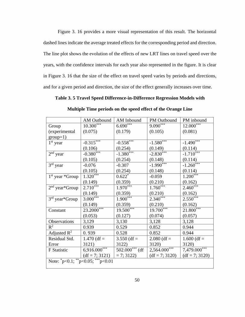
50
Figure 3. 16 provides a more visual representation of this result. The horizontal
dashed lines indicate the average treated effects for the corresponding period and direction.
The line plot shows the evolution of the effects of new LRT lines on travel speed over the
years, with the confidence intervals for each year also represented in the figure. It is clear
in Figure 3. 16 that the size of the effect on travel speed varies by periods and directions,
and for a given period and direction, the size of the effect generally increases over time.
Table 3. 5 Travel Speed Difference-in-Difference Regression Models with
Multiple Time periods on the speed effect of the Orange Line
AM Outbound AM Inbound PM Outbound PM inbound
Group
(experimental
group=1)
10.300***
(0.075)
6.690***
(0.179)
9.090***
(0.105)
12.000***
(0.081)
1st year -0.315***
(0.106)
-0.558***
(0.254)
-1.580***
(0.149)
-1.490***
(0.114)
2nd year -0.380***
(0.105)
-1.380***
(0.254)
-2.830***
(0.148)
-1.710***
(0.114)
3rd year -0.076
(0.105)
-0.307
(0.254)
-1.990***
(0.148)
-1.260***
(0.114)
1st year *Group 1.320***
(0.149)
0.622*
(0.359)
-0.059
(0.210)
1.200***
(0.162)
2nd year*Group 2.710***
(0.149)
1.970***
(0.359)
1.760***
(0.210)
2.460***
(0.162)
3rd year*Group 3.000***
(0.149)
1.900***
(0.359)
2.340***
(0.210)
2.550***
(0.162)
Constant 23.2000***
(0.053)
19.500***
(0.127)
19.700***
(0.074)
21.800***
(0.057)
Observations 3,129 3,130 3,128 3,128
R2 0.939 0.529 0.852 0.944
Adjusted R2 0. 939 0.528 0.852 0.944
Residual Std.
Error
1.470 (df =
3121)
3.550 (df =
3122)
2.080 (df =
3120)
1.600 (df =
3120)
F Statistic 6,916.000***
(df = 7; 3121)
502.000*** (df
= 7; 3122)
2,564.000***
(df = 7; 3120)
7,479.000***
(df = 7; 3120)
Note: *p<0.1; **p<0.05; ***p<0.01

51
Figure 3. 16 Predicted speed based on the DID models with multiple time periods
for the Orange line during weekday peak periods
For the Green line case, Table 3. 6 shows that most of the coefficients for Year *
Group of the DID estimators were positive and statistically significant, indicating that there
were increases in travel speed on the experimental roadway. The size of Year * Group
coefficients from the DID estimators were highest in the third year for all four models, but
there is no clear pattern of how the effect changes over time. Figure 3. 17 provides a visual
representation of the result. As shown in Figure 3. 17, for a given period and direction,
even though the point estimates of the effect differ from one year to the next, their
confidence intervals largely overlap, indicating the differences in the effect size over the
years are not statistically significant.

52
Table 3. 6 Results of Travel Speed Difference-in-Difference Regression
Models with multiple time periods of the Green Line Case
AM Outbound AM Inbound PM Outbound PM inbound
Group
(experimental
group=1)
10.500***
(0.595)
7.270***
(0.798)
4.350***
(0.186)
5.400***
(0.581)
1st year -1.130***
(0.589)
-0.480***
(0.799)
1.400***
(0.183)
-0.093***
(0.580)
2nd year -5.050***
(0.588)
-0.777***
(0.802)
1.190***
(0.182)
2.350***
(0.589)
3rd year -5.740***
(0.588)
-4.600***
(0.797)
0.794***
(0.183)
-1.110***
(0.577)
4th year -4.830***
(0.592)
-3.630***
(0.811)
0.887***
(0.184)
-1.680***
(0.583)
5th year -6.550***
(0.625)
-7.940***
(0.827)
0.208
(0.188)
-2.760***
(0.592)
1st year *Group 3.200***
(0.832)
0.112
(1.120)
-1.390***
(0.258)
-0.293
(0.811)
2nd year*Group 5.910***
(0.831)
1.450
(1.120)
-0.720***
(0.257)
-3.790***
(0.817)
3rd year*Group 7.060***
(0.834)
4.150***
(1.120)
3.250***
(0.260)
2.620***
(0.816)
4th year*Group 3.680***
(0.852)
0.329
(1.140)
2.300***
(0.262)
0.866
(0.827)
5th year*Group 3.200***
(1.060)
3.650***
(1.360)
2.660***
(0.267)
-0.204
(0.840)
Constant 44.900***
(0.432)
46.000***
(0.574)
55.500***
(0.133)
47.700***
(0.420)
Observations 2,773 2.833 2,884 2,922
R2 0.574 0.249 0.677 0.184
Adjusted R2 0.572 0.246 0.675 0.181
Residual Std.
Error
6.580 (df =
2761)
8.910 (df =
2821)
2.010 (df =
2872)
6.410 (df =
2910)
F Statistic 338.000*** (df
= 11; 2761)
85.000*** (df
= 11; 2821)
547.000*** (df
= 11; 2872)
59.600*** (df
= 11; 2910)
Note: *p<0.1; **p<0.05; ***p<0.01
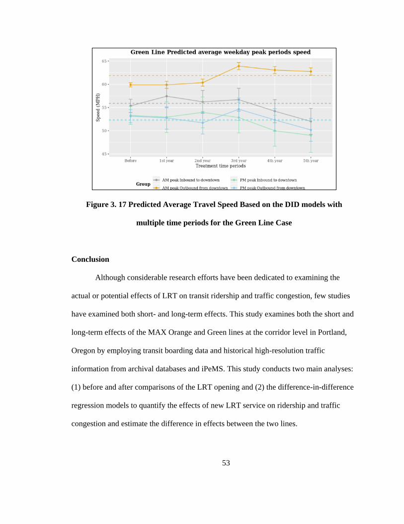
53
Figure 3. 17 Predicted Average Travel Speed Based on the DID models with
multiple time periods for the Green Line Case
Conclusion
Although considerable research efforts have been dedicated to examining the
actual or potential effects of LRT on transit ridership and traffic congestion, few studies
have examined both short- and long-term effects. This study examines both the short and
long-term effects of the MAX Orange and Green lines at the corridor level in Portland,
Oregon by employing transit boarding data and historical high-resolution traffic
information from archival databases and iPeMS. This study conducts two main analyses:
(1) before and after comparisons of the LRT opening and (2) the difference-in-difference
regression models to quantify the effects of new LRT service on ridership and traffic
congestion and estimate the difference in effects between the two lines.
54
A notable finding from the research is that the development of two LRT lines in
Portland,
Oregon has led to a large increase in transit ridership and a positive impact on relieving
traffic congestion. This study also finds that the effects on traffic congestion largely
persist over the years –keeping improving in the case of the Orange line and lacking a
clear pattern in the case of the Green line.
Specifically, the analysis on transit ridership indicates that after the opening of the
new light rail transit lines, boardings within the experimental corridor increased sharply
while those within the control corridor remained unchanged. The results of the ridership
DID base models demonstrate that the Orange and Green Lines contributed to an increase
of 6,404 and 7,225 riders on average, respectively. The crosstab of Green Line ridership
suggests that ridership increase mainly occurred in the first three years after its operation.
The travel speed models reveal that the new LRT lines have had a positive impact on
traffic speed, with the magnitude of the effects varying by peak periods and direction. For
the Orange Line, travel speed increased by between 1.35 and 2.35 mph, while for the
Green Line, travel speed increased by between 1.12 and 5.12 mph. The DID models with
multiple periods demonstrate that most yearly effects are positive and statistically
significant and that the size of the yearly effects changes over time. For the Orange Line,
the effect size on travel speed increases over time. For the Green Line, there is no clear
pattern in differences in the effect size over time.
The research demonstrates how high-resolution historical data makes it possible
to evaluate the impacts of transportation projects and policies. The spatial and temporal

55
high-resolution data make is possible to detect impact, which cannot be captured without
such dataset, on transportation system. The availability of detailed transportation data is
crucial to evaluate the effects and evolution of transportation policies and projects like
LRT. Such dataset makes it possible to conduct comprehensively temporal and spatial
evaluation of the effect. Thus, it would help fill a research gap and explain the conflicting
empirical results in previous studies because of different time frames and intervals or
geographical scales.

56
4. Effect of new LRT service on transit ridership and traffic congestion at the
regional level
Many cities in the U.S. have tilted transit investments toward LRT despite the
substantially higher cost, because transit with a separate right-of-way is commonly
viewed to be more likely to help relieve traffic congestion (Downs, 2005; Litman, 2014).
Though a considerable body of research has investigated transit ridership and congestion
effect of LRT, little research has examined the long-term effect of large transit projects
on transit ridership and traffic congestion at the regional level, and the causal relationship
between transit and traffic congestion and transit ridership is rarely analyzed in the
literature.
The New Starts program is a transit capital investment program administrated by
Federal Transit Administration (FTA). It primarily funds fixed guideway systems,
including light rail, commuter rail, and fixed guideway Bus Rapid Transit (BRT). To
apply for funding from New Starts, the cost of the transit project should be more than
$300 million, or the total New Starts funding sought should be no less than $100 million
(Federal Transit Administration, 2015). From 1998 to 2017, 55 New Starts transit
projects began operation across 27 UZAs and the total funding reached approximately
$20 billion. All projects competing for funding are selected based on their potential
effects on accessibility, mobility, congestion relief, land use changes, and cost-
effectiveness. Although the New Starts program has funded various projects across
UZAs, to my knowledge, no study has comprehensively examined the effect of these
projects on transit ridership and traffic congestion.

57
This study attempts to quantify the effect of new LRT service on transit ridership
and traffic congestion at the regional level. This study conducts an empirical analysis of
the impacts of new LRT lines on ridership and traffic congestion in three UAs that
constructed New Starts LRT projects from 1982 to 2017. To capture the effect of new
LRT lines on traffic, we use a synthetic control method to construct a “synthetic” control
UA that closely approximates the counterfactual ridership and traffic congestion scenario
in the absence of light rail projects. Results of this study provide empirical evidence for
the effect of large transit investment on traffic congestion and contribute to the ongoing
debates concerning the effectiveness of LRT service to increase transit ridership and
relieve traffic congestion across Urban Areas in the U.S.
Methodology
The Synthetic control method (SCM) was original proposed by Abadie and
Gardeazabal (2003). The SCM circumvents two shortcomings of traditional comparative
case studies (Abadie et al., 2012). First, in traditional comparative case studies,
comparison cases selection largely relies on the subjective measures of affinity between
treated cases and control cases in most applications, and such ambiguity of comparison
cases selection is hard to eliminate. The synthetic control method constructs a “synthetic”
control case to compare with the treated case with a data-driven approach. The data-
driven procedures reduce the discretion of control UAs selection. Second, characteristics
of the “synthetic” control case are much more similar to the characteristics of the treated
UA than any single actual control case. The synthetic control method constructs a
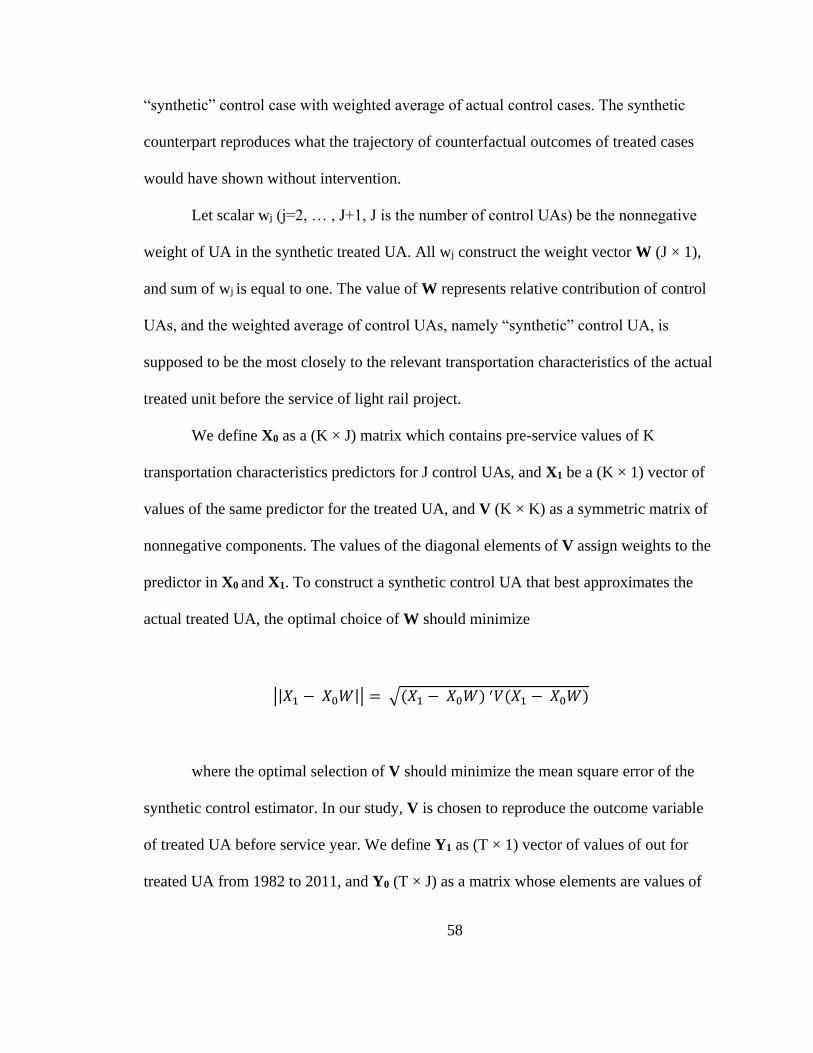
58
“synthetic” control case with weighted average of actual control cases. The synthetic
counterpart reproduces what the trajectory of counterfactual outcomes of treated cases
would have shown without intervention.
Let scalar wj (j=2, … , J+1, J is the number of control UAs) be the nonnegative
weight of UA in the synthetic treated UA. All wj construct the weight vector W (J × 1),
and sum of wj is equal to one. The value of W represents relative contribution of control
UAs, and the weighted average of control UAs, namely “synthetic” control UA, is
supposed to be the most closely to the relevant transportation characteristics of the actual
treated unit before the service of light rail project.
We define X0 as a (K × J) matrix which contains pre-service values of K
transportation characteristics predictors for J control UAs, and X1 be a (K × 1) vector of
values of the same predictor for the treated UA, and V (K × K) as a symmetric matrix of
nonnegative components. The values of the diagonal elements of V assign weights to the
predictor in X0 and X1. To construct a synthetic control UA that best approximates the
actual treated UA, the optimal choice of W should minimize
||𝑋1 − 𝑋0𝑊|| = √(𝑋1 − 𝑋0𝑊) ′𝑉(𝑋1 − 𝑋0𝑊)
where the optimal selection of V should minimize the mean square error of the
synthetic control estimator. In our study, V is chosen to reproduce the outcome variable
of treated UA before service year. We define Y1 as (T × 1) vector of values of out for
treated UA from 1982 to 2011, and Y0 (T × J) as a matrix whose elements are values of
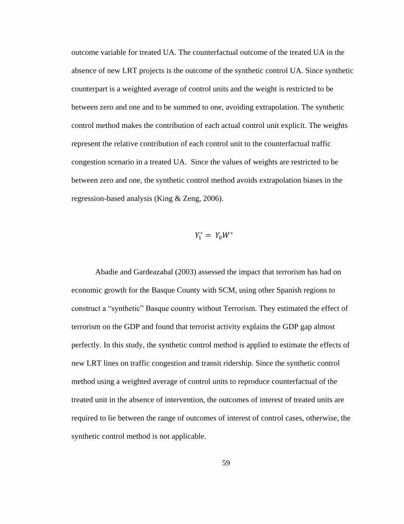
59
outcome variable for treated UA. The counterfactual outcome of the treated UA in the
absence of new LRT projects is the outcome of the synthetic control UA. Since synthetic
counterpart is a weighted average of control units and the weight is restricted to be
between zero and one and to be summed to one, avoiding extrapolation. The synthetic
control method makes the contribution of each actual control unit explicit. The weights
represent the relative contribution of each control unit to the counterfactual traffic
congestion scenario in a treated UA. Since the values of weights are restricted to be
between zero and one, the synthetic control method avoids extrapolation biases in the
regression-based analysis (King & Zeng, 2006).
𝑌1∗ = 𝑌0𝑊∗
Abadie and Gardeazabal (2003) assessed the impact that terrorism has had on
economic growth for the Basque County with SCM, using other Spanish regions to
construct a “synthetic” Basque country without Terrorism. They estimated the effect of
terrorism on the GDP and found that terrorist activity explains the GDP gap almost
perfectly. In this study, the synthetic control method is applied to estimate the effects of
new LRT lines on traffic congestion and transit ridership. Since the synthetic control
method using a weighted average of control units to reproduce counterfactual of the
treated unit in the absence of intervention, the outcomes of interest of treated units are
required to lie between the range of outcomes of interest of control cases, otherwise, the
synthetic control method is not applicable.

60
Data and sample
This study uses annual Urban Area (UA) level panel data from 1982 to 2017. A
primary data source is the Urban Mobility Report (UMR) from Texas A&M
Transportation Institute. The primary outcomes of interest are traffic congestion and
transit ridership, measured as Travel Time Index (TTI) and Public Transit Annual
Passenger Miles (PTAPM) respectively. TTI is the ratio of the peak-period travel time
compared to the free-flow travel time. A TTI of 1.20 indicates a 10‐minute free‐flow trip
takes 12 minutes in the peak period. In the dataset, TTI is available from 1982 to 2017;
PTAPM is available from 1982 to 2011 (Schrank et al., 2012, 2019). The UMR panel
dataset also includes other characteristics for each UA: population, auto travel cost,
average state gasoline cost, average state diesel cost, freeway lane-miles, arterial street
lane-miles, peak period travelers, commuters. Besides, this study collects employment
and income data from the Bureau of Economic Analysis.
Since traffic congestion is more severe in large UAs, this study focuses on large
UAs. In the UMR dataset, there are 47 UAs in the very large and large category,
including 15 UAs with population over 3 million and 32 UAs with population between 1
million and 3 million.
This study attempts to estimate the effect of New Starts LRT projects on transit
ridership and traffic congestion. Of these 47 UAs, 20 UAs that do not receive New Starts
support are potential control UAs. After reviewing transportation systems in these 20
UAs, I find that there are 8 UAs with rail-like transit service, including light rail, heavy
rail, commuter rail, monorail and automated guideway. Thus, these 8 UAs cannot be used

61
as control units. Finally, 12 UAs without any types of rail-based transit service are
identified as control units, listed in Table 4. 1. These 12 UAs make up the donor pool for
the SCM analysis. For each treated UA, these 12 control UAs are used to construct its
synthetic counterpart to examine what the transit ridership and traffic congestion would
have been in the absence of light rail projects.
Table 4. 1 Control urban areas
Urban Area TTI in 2017 PTAPM (million) in
2011
Cincinnati OH-KY-IN 1.17 112.00
Columbus OH 1.19 72.30
Detroit MI 1.24 309.00
Indianapolis IN 1.18 39.90
Kansas City MO-KS 1.15 69.50
Louisville KY-IN 1.18 65.90
Milwaukee WI 1.17 154.50
Nashville-Davidson TN 1.22 69.90
Providence RI-MA 1.17 96.20
Raleigh-Durham NC 1.17 100.40
San Antonio TX 1.23 207.00
Tampa-St. Petersburg FL 1.22 146.50
The synthetic control method requires a certain period of pre-treatment data to
construct the synthetic control counterpart. The existing studies generally use at least 10
years of pre-treatment data (Abadie et al., 2011). The data used in this study began in
1982. To ensure enough years in the pre-treatment period, this study selects UAs that
began LRT service in and after 1992 as treated UAs. Besides, the SCM approach restricts
the weights of the actual control units to be between zero and one to avoid extrapolation
when constructing the “synthetic” control unit. Thus, UAs with values of outcomes of

62
interest outside the range of values of outcome of interests of the control units are
excluded in this analysis. Taking the Seattle UA as an example, its TTI is much higher
than those of the control UAs, shown in Figure 4. 1.
Figure 4. 1 TTI in Seattle WA and control UAs
After excluding UAs with outcomes of interest outside the range of control UAs,
there are three UAs remaining, including Charlotte NC-SC and St. Louis MO-IL, and
Virginia Beach VA. For each treated UA, the SCM approach is employed to examine the
effect of LRT on transit ridership and traffic congestion. Because the operation year of
LRT in Virginia Beach VA is 2011 and PTAPM is only available from 1982-2011, this
study does not investigate the effect of LRT on transit ridership in Virginia Beach VA.
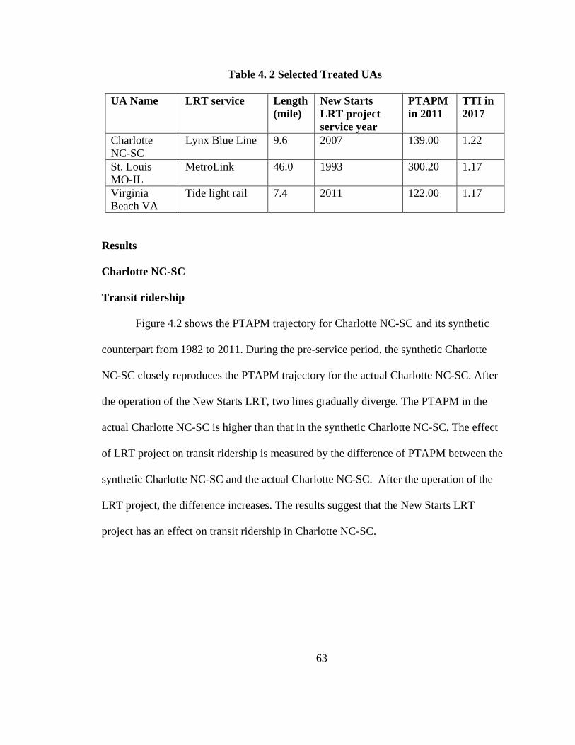
63
Table 4. 2 Selected Treated UAs
UA Name LRT service Length
(mile)
New Starts
LRT project
service year
PTAPM
in 2011
TTI in
2017
Charlotte
NC-SC
Lynx Blue Line 9.6 2007 139.00 1.22
St. Louis
MO-IL
MetroLink 46.0 1993 300.20 1.17
Virginia
Beach VA
Tide light rail 7.4 2011 122.00 1.17
Results
Charlotte NC-SC
Transit ridership
Figure 4.2 shows the PTAPM trajectory for Charlotte NC-SC and its synthetic
counterpart from 1982 to 2011. During the pre-service period, the synthetic Charlotte
NC-SC closely reproduces the PTAPM trajectory for the actual Charlotte NC-SC. After
the operation of the New Starts LRT, two lines gradually diverge. The PTAPM in the
actual Charlotte NC-SC is higher than that in the synthetic Charlotte NC-SC. The effect
of LRT project on transit ridership is measured by the difference of PTAPM between the
synthetic Charlotte NC-SC and the actual Charlotte NC-SC. After the operation of the
LRT project, the difference increases. The results suggest that the New Starts LRT
project has an effect on transit ridership in Charlotte NC-SC.

64
(a) Trends in PTAPM
(b) Gap between Treatment and Synthetic Control
Figure 4. 2 PTAPM in Charlotte NC-SC

65
Traffic congestion
Figure 4. 3 visualizes the TTI trajectory for Charlotte NC-SC and its synthetic
counterpart for the 1982-2017 period. During the pre-service period, the synthetic
Charlotte NC-SC almost precisely reproduces the TTI for the Charlotte NC-SC. After the
operation of the LRT service, TTI in the actual Charlotte NC-SC increased in the first
year and then decreased, while TTI of the synthetic Charlotte NC-SC decreased first and
then increased. Two lines intersect around 2016.
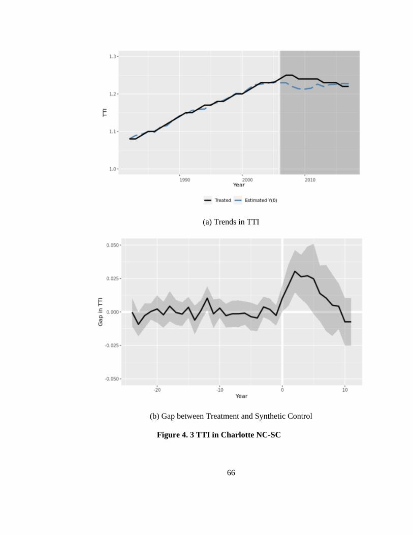
66
(a) Trends in TTI
(b) Gap between Treatment and Synthetic Control
Figure 4. 3 TTI in Charlotte NC-SC

67
Our estimate of the effect of new LRT service on traffic congestion is measured
by the difference of TTI between the synthetic Charlotte NC-SC and the actual Charlotte
NC-SC, shown in Figure 4. 3. After the operation of the LRT service, the difference first
widens and then gradually narrows and becomes negative around 2016. Our results
suggest that the new LRT service has had a negative effect on traffic congestion, that is, it
worsens the congestion measured by TTI.
St. Louis MO-IL
Transit ridership
Figure 4. 4 shows the PTAPM trajectory for St. Louis MO-IL and its synthetic
counterpart from 1982 to 2011, and the difference in PTAPM between the actual St.
Louis MO-IL and the synthetic St. Louis MO-IL. The synthetic St. Louis MO-IL closely
reproduces the PTAPM for St. Louis MO-IL during the pre-treatment period. After the
operation of the LRT service, the two lines substantially diverge. After the operation of
the new LRT project, the difference increases over time. The results suggest that the new
LRT project has a pronounced positive effect on transit ridership in St. Louis MO-IL.

68
(a) Trends in PTAPM
(b) Gap between Treatment and Synthetic Control
Figure 4. 4 PTAPM in St. Louis Mo-IL

69
Traffic congestion
Figure 4. 5 shows the TTI trajectory of St. Louis MO-IL and its synthetic
counterpart for the 1982-2017 period. During pre-treatment period, the synthetic St.
Louis MO-IL closely reproduces the TTI for St. Louis MO-IL. In the first five years
immediately following the operation of new LRT service, TTI in the actual St. Louis
MO-IL and its synthetic counterpart is close. From 1998 onward, the gap between the
two lines varies over time, but constantly stays negative, indicating an effect of the New
Starts LRT projects on reducing congestion (lowering TTI) for the St. Louis MO-IL UA.

70
(a) Trends in TTI
(b) Gap between Treatment and Synthetic Control
Figure 4. 5 TTI in St. Louis Mo-IL

71
Virginia Beach VA
Traffic congestion
Figure 4. 6 shows the TTI for Virginia Beach VA and its synthetic counterpart
from 1982 to 2017. The synthetic Virginia Beach VA exactly reproduces the TTI for the
actual Virginia Beach VA during the pre-treatment period. After the operation of LRT
service, the two lines are still close. The effect of new LRT service on traffic congestion
is measured by the difference between the actual Virginia Beach VA and its synthetic
Virginia Beach VA. The difference is small after the operation of the new LRT service.
The results suggest no effect of New Start LRT service on traffic congestion in Virginia
Beach VA.

72
(a) Trends in TTI
(b) Gap between Treatment and Synthetic Control
Figure 4. 6 TTI in Virginia Beach VA

73
Table 4. 3 GSCM Results across UAs shows the analysis results of three UAs.
The average treated effects and p-values are calculated with the generalized synthetic
control method (Xu, 2017). The results suggest that the effect of the new LRT projects on
transit ridership and traffic congestion varies across UAs. For transit ridership, the New
Starts LRT service increases transit ridership in two UAs: the effect is significant in St.
Louis MO-IL and the effect is not significant in Charlotte NC-SC. This probably because
the New Starts LRT project that began service in 2007 is small in Charlotte NC-SC.
Though this New Starts LRT service is the first trail line in Charlotte NC-SC, it is only a
9.6-mile route line, accounting for a small proportion of transportation supply.
For traffic congestion, the effects of the new LRT service on traffic congestion are
not significant, though the figures for traffic congestion show that there is a relief effect
on traffic congestion. One reason may be that driving mode is the dominant mode in
these UAs and transits only accounts for a limited share in daily travel.
Table 4. 3 GSCM Results across UAs
UA Name
Average Treated Effect
PTAPM (p value) TTI (p value)
Charlotte NC-SC 18.38 million (0.416) 0.013 (0.053)
St. Louis MO-IL 93.31 million (0.0330) -0.014 (0.556)
Virginia Beach -0.003(0.931)
Conclusions
This chapter of the dissertation focuses on the effects of New Starts LRT Projects
on transit ridership and traffic congestion at the regional level. This study applies the

74
SCM to quantify and compare transit ridership and traffic conditions before and after the
launch of new LRT projects in three UAs.
In this study, the effects of new LRT project on transit ridership and traffic
congestion are different across UAs. These are consistent with expectations (Beaudoin et
al., 2015). There is regional spatial heterogeneity across UAs. The effects on transit
ridership are significant, while the effects on traffic congestion are not significant. LRT
only accounts for a limited share in commuting travel. Thus, the construction of new LRT
service is hard to exact a pronounced relief effect at the regional level. The results also
indicate that the effect of new LRT service on transit ridership and traffic congestion
changes over time at the regional level.
This study illustrates the advantages of using the SCM approach. The data-driven
procedures for constructing synthetic unit reduce the subjective selection of comparison
units. Most synthetic control UAs reproduce the counterfactual of the treated UA in the
absence of new LRT projects. This study also demonstrates the applicability of synthetic
control method on studying the effects of transportation policies and investments at the
UA-level and how it complements and facilitate comparative case studies in the
transportation field. The SCM provides a counterfactual analysis and the results are much
more intuitive to interpret than previous research results using a model-based approach or
regression-based empirical analysis.
The approach, however, has some limitations. First, though the synthetic control
method provides a convenient way to create a comparable control unit, the outcome of
interest should be within the range of outcomes of actual control units due to positive

75
weight restriction. Second, in this study, most large UAs have LRT and therefore there
are a limited number of large UAs in the donor pool, which makes large UAs unable to
be analyzed with the synthetic control method. Third, whether the SCM approach can
construct a comparable synthetic largely depends on the donor pool. If a synthetic
counterpart could not be constructed with the donor pool, a solid conclusion could not be
drawn. And there are few ways to say definitively whether a counterfactual estimate is
acceptable or not.

76
5. Discussions and takeaways
This research provides a closer look at the impact of new LRT service on transit
ridership and traffic congestion at different geographical levels by utilizing newer data
sources. At the corridor level, using transit boarding data and high-resolution historical
traffic information from archival databases and iPeMS, this study comprehensively
investigates the short- and long-term effects of LRT through case studies of two LRT
lines in Portland, Oregon region. Using a quasi-experimental design, this study estimated
the effects of LRT on transit ridership as well as traffic congestion. In contrast to existing
research, this study used high-resolution transit and travel speed data from a longer time
period. Such dataset allows for comprehensively temporal and spatial evaluation. For
each LRT line, transit ridership and traffic conditions before and after opening were
compared and difference-in-difference (DID) regression models were estimated in order
to quantify the effects. The results demonstrated that both LRT lines increased transit
ridership in the short- and long-term. The Orange Line contributed to an increase of 6,404
riders on average and the Green Line 7,225, and the effect is significant especially in the
first three years. Also, it is estimated that travel speed increased by 1.35~2.35 mph for the
Orange Line and 1.12~5.12 mph for the Green Line. Although LRT relieved traffic
congestion in the short-term, it may have no significant effect on traffic congestion in the
long-term, probably due to induced traffic demand. The effects of LRT varied by LRT
lines because of various local land use and transportation systems.
Generally, at the corridor level, my work may contribute in terms of literature and
data handling. In addition to contributing to the literature on the effects of transit in terms

77
of travel ridership, speed and congestion, the results of this study demonstrate how high-
resolution archival transportation data enable analyses that had been previously
impossible. The growing availability of transportation data of high temporal and spatial
resolution over a long time period provides a unique opportunity to evaluate the effects
and evolution of transportation policies and projects like LRT, which helps to explain the
seemingly conflicting empirical results of existing studies.
However, several important points are worth exploring further. But limited to the
focus and scope of this dissertation, I do not give them in-depth discussion. As mentioned
earlier, “induced traffic demand” is one of the keys for traffic effect evaluation,
especially for the causal inference between the launch of transit and potential traffic
congestion alleviation in the long term. I find evidence that in the long term, the effect of
LRT on traffic congestion will be weaker than that of the first three years, and this is
probably because people adjust their behaviors (change traffic routes, move home or
work location, etc.) and for high demand areas and inbound/outbound option (AM
inbound or PM outbound), long term effect (three years or more) tends to be
insignificant. Based on the analysis at the corridor level, I anticipate that the future
research will provide more evidence and insights on the cutting point of long term from
short term and LRT long term corridor traffic effect mechanism (e.g., interaction between
induced traffic demand, local land use & transportation systems, and people adjustment
of mismatching).
Study conducts an empirical analysis of the impacts of new light rail transit (LRT)
lines on traffic congestion in three UAs at the regional level. To capture the transit

78
ridership and traffic congestion effect of new LRT lines, we use a synthetic control
method to construct a “synthetic” control UA that closely approximates the
counterfactual transit ridership and traffic congestion scenario in the absence of light rail
projects. Results indicated that New Starts LRT projects contributed to transit ridership in
most UAs but they did relieve traffic congestion in limited UAs, and that the effect
changed over time and varied across UAs. The analysis of LRT miles indicates that UAs
with New Starts LRT projects are more likely to build more LRT.
To quantify the regional level effect of LRT on traffic ridership and congestion,
instead of applying traditional case studies, I select to use SCM method to do the
comparison. Different from sampling-based inference (e.g. DID), SCM is specifically
designed to facilitate the evaluation of policy intervention or events taking place at an
aggregate level (e.g. school districts, cities, countries). Although SCM is an appropriate
method for the regional level analysis, it has been technically difficult to draw
fundamentally solid and detailed causal inference comparable to what can be done at the
corridor level. In Chapter 4, SCM was used to visualize the long-term trend of LRT on
traffic ridership and congestion, which provided evidence that LRT region may subject to
more severe traffic congestion in the long run. Moreover, given that the 3 UAs are
subject to different land use and transportation systems, further studies may be conducted
to explore why LRT in different regions contributes to different traffic effects. Last but
not least, although the results show some evidence that the traffic congestion has become
worse after the operation of the new LRT service, LRT undoubtedly has provided local

79
people with more economic opportunities and social benefits (e.g. easy accessibility and
mobility).
This study provides some takeaways for the practitioners in transportation policy
and planning. Not only quantifying the benefits (e.g. increase ridership and speed, relieve
congestion in the short term), this research also provides evidence of the evolution of the
effect of new LRT service on transit ridership and traffic congestion. These findings may
help practitioners to make potential transit investment decision. The findings of this study
indicate the short and long-term potential effects, including transport ridership, travel
speed and traffic congestion, of new LRT service, and hence will be useful for
practitioners to optimize transit system to maximize benefits.
This study also makes contributions to the transport modeling and traveler
behavior research, and may help to fill the gap of existing inconsistent documents. First,
this study illustrates how high-resolution archival transportation data facilitate impact
analysis of transportation policies and projects previously difficult. Due to the lack of
detailed travel time data, most existing studies have to use approximate measurements of
traffic congestion, such as AADT and VMT. The high-resolution data make it possible to
use direct measurements of congestion and trace the changes of the effect on traffic
congestion. Second, this study illustrates an application of novel methods like SCM to
study the effects of semi-unique policies and projects, like New Starts projects. Despite
the widespread availability of data at the regional level, comparative studies with
rigorous methodology at the regional level are rare. A primary reason is that it is hard to
find a comparable control region. By constructing a “synthetic” control unit that closely

80
approximates the counterfactual scenario in the absence of treatment with the data-driven
procedure, the SCM addresses the difficulty in control unit selection in comparative
studies. Another advantage of the SCM over cross-sectional and panel data analysis is
that it can trace the changes of the outcomes of interest. Lastly, this study helps explain
the inconsistent results of existing research and provide additional in-depth understanding
of the effects of LRT. Results of the evolution of the effects over time explain the
inconsistent evidence due to different time dimensions. In addition, this dissertation
analyzes the effects at different levels, which could explain the inconsistency resulted
from differential spatial scales.

81
References
Abadie, A., Diamond, A., & Hainmueller, J. (2011). Synth: An r package for synthetic
control methods in comparative case studies. Journal of Statistical Software,
42(13). http://papers.ssrn.com/sol3/papers.cfm?abstract_id=1958891
Abadie, A., Diamond, A., & Hainmueller, J. (2012). Synthetic control methods for
comparative case studies: Estimating the effect of California’s tobacco control
program. Journal of the American Statistical Association.
http://amstat.tandfonline.com/doi/abs/10.1198/jasa.2009.ap08746
Abadie, A., & Gardeazabal, J. (2003). The economic costs of conflict: A case study of the
Basque Country. The American Economic Review, 93(1), 113–132.
Aftabuzzaman, M., Currie, G., & Sarvi, M. (2010). Modeling the spatial impacts of
public transport on traffic congestion relief in Melbourne, Australia.
Transportation Research Record: Journal of the Transportation Research Board,
2144(1), 1–10.
Anderson, M. L. (2013). Subways, Strikes, and Slowdowns: The Impacts of Public
Transit on Traffic Congestion (Working Paper No. 18757). National Bureau of
Economic Research. http://www.nber.org/papers/w18757
APTA. (2017). APTA 2017 Public Transportation Fact Book.
https://www.apta.com/resources/statistics/Pages/transitstats.aspx
Baum-Snow, N., & Kahn, M. E. (2005). Effects of Urban Rail Transit Expansions:
Evidence from Sixteen Cities, 1970-2000 [with Comment]. Brookings-Wharton
Papers on Urban Affairs, 147–206.

82
Beaudoin, J., Farzin, Y. H., & Lin, C. Y. (2015). Evaluating public transit investment in
congested cities.
http://www.des.ucdavis.edu/faculty/Lin/transit_congestion_paper.pdf
Beaudoin, J., Farzin, Y. H., & Lin, C.-Y. C. (2014). Evaluating Public Transit Investment
in Congested Cities. Working paper, University of California at Davis.
http://www.des.ucdavis.edu/faculty/Lin/transit_congestion_paper.pdf
Beaudoin, J., & Lin, C.-Y. C. (2018). The effects of public transit supply on the demand
for automobile travel. Journal of Environmental Economics and Management, 88,
447–467. https://doi.org/10.1016/j.jeem.2018.01.007
Bhattacharjee, S., & Goetz, A. R. (2012). Impact of light rail on traffic congestion in
Denver. Journal of Transport Geography, 22, 262–270.
https://doi.org/10.1016/j.jtrangeo.2012.01.008
Cao, X. (Jason), & Schoner, J. (2014a). The influence of light rail transit on transit use:
An exploration of station area residents along the Hiawatha line in Minneapolis.
Transportation Research Part A: Policy and Practice, 59, 134–143.
https://doi.org/10.1016/j.tra.2013.11.001
Cao, X. (Jason), & Schoner, J. (2014b). The influence of light rail transit on transit use:
An exploration of station area residents along the Hiawatha line in Minneapolis.
Transportation Research Part A: Policy and Practice, 59, 134–143.
https://doi.org/10.1016/j.tra.2013.11.001
Cervero, R. (1994). Transit-based housing in California: Evidence on ridership impacts.
Transport Policy, 1(3), 174–183. https://doi.org/10.1016/0967-070X(94)90013-2

83
Cervero, R. (2002). Induced Travel Demand: Research Design, Empirical Evidence, and
Normative Policies. Journal of Planning Literature, 17(1), 3–20.
https://doi.org/10.1177/088122017001001
Ding, C., Lin, Y., & Liu, C. (2014). Exploring the influence of built environment on tour-
based commuter mode choice: A cross-classified multilevel modeling approach.
Transportation Research Part D: Transport and Environment, 32, 230–238.
Downs, A. (2005). Still stuck in traffic: Coping with peak-hour traffic congestion.
Brookings Institution Press.
https://books.google.com/books?hl=en&lr=&id=ckLcxEb5tM8C&oi=fnd&pg=P
R7&dq=Still+stuck+in+traffic+&ots=fGn8HUyK0V&sig=n38DQDcineVOTACf
PEIZI26nHmc
Ewing, R., & Cervero, R. (2010). Travel and the Built Environment—A Meta-Analysis.
Journal of the American Planning Association, 76(3), 265–294.
Ewing, R., Tian, G., Spain, A., & Goates, J. P. (2014). Effects of Light-Rail Transit on
Traffic in a Travel Corridor. Journal of Public Transportation, 17(4), 93.
Federal Transit Administration. (2015, October 2). About the Program [Text]. Federal
Transit Administration. https://www.transit.dot.gov/funding/grant-
programs/capital-investments/about-program
Giuliano, G. (2004). Land Use Impacts of Transportation Investments-Highway and
Transit. In The Geography of Urban Transportation (Third, pp. 237–273).
https://trid.trb.org/view.aspx?id=756066

84
Giuliano, G., Chakrabarti, S., & Rhoads, M. (2015). Using Regional Archived
Multimodal Transportation System Data for Policy Analysis: A Case Study of the
LA Metro Expo Line. Journal of Planning Education and Research,
0739456X15604444. https://doi.org/10.1177/0739456X15604444
Hansen, S., Byrd, A., Delcambre, A., Rodriguez, A., Matthews, S., & Bertini, R. L.
(2005). PORtal: An on-line regional transportation data archive with
transportation system management applications. Department of Civil and
Environmental Engineering, Nohad A.
King, G., & Zeng, L. (2006). The dangers of extreme counterfactuals. Political Analysis,
14(2), 131–159.
Litman, T. (2014). Critique of “Transit Utilization and Traffic Congestion: Is There a
Connection?” http://trid.trb.org/view.aspx?id=1304849
Lo, S.-C., & Hall, R. W. (2006). Effects of the Los Angeles transit strike on highway
congestion. Transportation Research Part A: Policy and Practice, 40(10), 903–
917.
Lund, H., Willson, R. W., & Cervero, R. (2006). A RE-EVALUATION OF TRAVEL
BEHAVIOR IN CALIFORNIA TODS. Journal of Architectural and Planning
Research, 23(3), 247–263.
Nelson, P., Baglino, A., Harrington, W., Safirova, E., & Lipman, A. (2007). Transit in
Washington, DC: Current benefits and optimal level of provision. Journal of
Urban Economics, 62(2), 231–251. https://doi.org/10.1016/j.jue.2007.02.001

85
Noland, R. B., & Lem, L. L. (2002). A review of the evidence for induced travel and
changes in transportation and environmental policy in the US and the UK.
Transportation Research Part D: Transport and Environment, 7(1), 1–26.
https://doi.org/10.1016/S1361-9209(01)00009-8
NTD. (2000). 1999 National Transit Summaries and Trends [Text].
https://www.transit.dot.gov/sites/fta.dot.gov/files/docs/NTST%20for%20RY%20
1999.pdf
NTD. (2018). 2017 National Transit Summaries and Trends [Text].
https://www.transit.dot.gov/sites/fta.dot.gov/files/docs/ntd/130636/2017-national-
transit-summaries-and-trends.pdf
Pickerell, D. (2001). Induced Demand: Definition, Measurement an Significance.
Working Together to Address Induced Demand, 26.
Schrank, D., Eisele, B., & Lomax, T. (2012). TTI’s 2012 urban mobility report. Texas
A&M Transportation Institute. The Texas A&M University System.
http://media2.kjrh.com/html/pdfs/2012urbanmobilityreport.pdf
Schrank, D., Eisele, B., & Lomax, T. (2019). 2019 URBAN MOBILITY REPORT.
https://static.tti.tamu.edu/tti.tamu.edu/documents/mobility-report-2019.pdf
Small, K. A., & Verhoef, E. T. (2007). The economics of urban transportation.
Routledge.
https://books.google.com/books?hl=en&lr=&id=6HGBAgAAQBAJ&oi=fnd&pg
=PT6&dq=The+Economics+of+Urban+Transportation.&ots=S55a6D8y5C&sig=
qoffkZzyiSDc3DAgJMhZmlabMCk

86
Sun, C., Zhang, W., Fang, X., Gao, X., & Xu, M. (2019). Urban public transport and air
quality: Empirical study of China cities. Energy Policy, 135, 110998.
https://doi.org/10.1016/j.enpol.2019.110998
Winston, C., & Langer, A. (2006). The effect of government highway spending on road
users’ congestion costs. Journal of Urban Economics, 60(3), 463–483.
https://doi.org/10.1016/j.jue.2006.04.003
Xu, Y. (2017). Generalized synthetic control method: Causal inference with interactive
fixed effects models. Political Analysis, 25(1), 57–76.
Yu, H., Wang, P., Zheng, H., Luo, J., & Liu, J. (2020). Impacts of congestion on
healthcare outcomes: An empirical observation in China. Journal of Management
Analytics, 7(3), 344–366. https://doi.org/10.1080/23270012.2020.1731720